Universal amplitude in density-force relations for polymer chains in confined geometries: Massive field theory approach.

Abstract

The universal density-force relation is analyzed and the correspondent universal amplitude ratio $B_{real}$ is obtained using the massive field theory approach in fixed space dimensions $d=3$ up to one-loop order. The layer monomer density profiles of ideal chains and real polymer chains with excluded volume interaction in a good solvent between two parallel repulsive walls, one repulsive and one inert wall are obtained. Besides, taking into account the Derjaguin approximation the layer monomer density profiles for dilute polymer solution confined in semi-infinite space containing mesoscopic spherical particle of big radius are calculated. The last mentioned situation is analyzed for both cases when wall and particle are repulsive and for the mixed case of repulsive wall and inert particle. The obtained results are in good agreement with previous theoretical results and with the results of Monte Carlo simulations.

The investigation of polymer solution near the surfaces and in film geometries or mesoscopic particles dissolved in the solution is a task of great interest from theoretical and application point of view.

The monomer density profiles of dilute polymer solution bounded by a planar repulsive wall has a depletion region of mesoscopic width of order of the coil size $R_{x}\approx N^{\nu}$ (where $N$ is the number of monomers per chain), and for the distances $\tilde{z}$ from the wall that are small compared to this width but bigger than microscopic lengths of monomer size $\tilde{l}$ the profile increases as

$$\rho(\tilde{z})\sim\tilde{z}^{\frac{1}{\nu}}$$

with Flory exponent $\nu$ ($\nu$ is $1/2$ for ideal polymer chains and $\nu\approx 0.588$ for polymer chains with excluded volume interaction (EVI)). This remarkable theoretical predictions was proposed by Joanny, Leibler and de Gennes JLG . They also mentioned that the monomer density close to the wall is proportional to the force per unit area which the polymer solution exerts on the wall. But, for the first time a complete quantitative expression for the universal density-force relation was obtained by Eisenriegler on the basis of $\epsilon$- expansion up to first order in E97 . As was mentioned in E97 , the correspondent density-force relations with the same universal amplitude $B$ are valid for the different cases: 1) a single polymer chain with one end (or both ends) fixed in the half space bounded by the wall; 2) a single chain trapped in the slit of two walls; 3) for the case of dilute and semi-dilute solution of free polymer chains in a half space; 4) for the case of polymer chain in a half space containing a mesoscopic particle of arbitrary shape. The verification of the universal density-force relation was performed by simulation techniques using an off-lattice bead-spring model of a polymer chain trapped between two parallel repulsive walls MB98 and by the lattice Monte Carlo algorithm on a regular cubic lattice in three dimensions HG04 . Unfortunately, the obtained results of Monte Carlo simulations in MB98 are much higher $B_{MC}>2.48$ than theoretical predictions $B_{\epsilon}\approx 1.85$ obtained in E97 . As it was mentioned in MB98 , there is a systematic decrease of $B_{eff}$ with increasing the distance $L$ between the walls. In accordance with it some rough linear extrapolation with plotting $B_{eff}$ versus $1/\sqrt{L}$ which yields an extrapolated result $B\sim 1.4$ was performed in MB98 . Recent numerical results based on the lattice Monte Carlo algorithm on a regular cubic lattice gives the value $B\approx 1.70\pm 0.08$ which is smaller than previous theoretical predictions. This all indicates that the above mentioned task still have a lot of open questions and the present paper tries to give answers for some of them.

The present paper is devoted to investigation of the universal density-force relation and calculation of the universal amplitude $B$ in the framework of the massive field theory approach. The massive field theory approach gives better agreement with the experimental data and the results of Monte Carlo calculations as it was shown in the case of infinite Par80 ; Parisi , semi-infinite DSh98 systems, and specially in the case of dilute polymer solutions in semi-infinite geometry U06 and confined geometry DU09 . As was mentioned above, the knowledge of the universal amplitude $B$ allows to obtain the monomer density profiles for whole class of different systems (cases 1)-4)). Besides, it should be mentioned that the universal density-force relation is valid not only for the case of polymer chains trapped in between two repulsive walls but also for the mixed case of one repulsive and one inert wall.

We consider a dilute polymer solution, where different polymer chains do not overlap and the behavior of such polymer solution can be described by a single polymer chain. As it is known, the single polymer chain can be modeled by the model of random walk and this corresponds to the ideal chain at $\theta$-solvent or self-avoiding walk for the real polymer chain with EVI for temperatures above the $\theta$-point. Taking into account the polymer-magnet analogy developed by deGennes , their scaling properties in the limit of an infinite number of steps $N$ may be derived by a formal $n\to 0$ limit of the field theoretical $\phi^{4}$ $O(n)$- vector model at its critical point. It should be mentioned that $1/N$ plays the role of a critical parameter analogous to the reduced critical temperature in magnetic systems. The role of a second critical parameter plays the deviation from the adsorption threshold $(c\propto(T-T_{a})/T_{a})$ (where $T_{a}$ is adsorption temperature). The value $c$ corresponds to the adsorption energy divided by $k_{B}T$ (or the surface enhancement constant in field theoretical treatment). The adsorption threshold for long-flexible polymer chains, where $1/N\to 0$ and $c\to 0$ is a multicritical phenomenon.

In order to obtain the universal amplitude $B$ in universal monomer-density relation let’s consider the single polymer chain with one end fixed fluctuating near the repulsive wall such that $(\tilde{l}<<\tilde{z}<<z<<R_{x})$.

The correspondent layer monomer densities $\rho_{\lambda}(\tilde{z})$ defined by E97 is:

$$\rho_{\lambda}(\tilde{z})d\tilde{z}=\frac{(R_{x})^{1/\nu}}{N}dN_{\lambda}(\tilde{z}),$$ (1)

where $dN_{\lambda}(\tilde{z})$ is the number of monomers in the layer between $\tilde{z}$ and $\tilde{z}+d\tilde{z}$, $R_{x}$ is the projection of the end to end distance ${\bf R}$ onto the direction of $x$ axis. Besides, $\rho_{\lambda}$ is obtained from monomer density $\rho(\tilde{{\bf r}},\tilde{z})$ after integration over the $d-1$ components parallel to the wall. The scaling dimension of $\rho(\tilde{{\bf r}},\tilde{z})$ is $l^{1/\nu-d}$ and equals the ordinary dimensions of the quantity

$${\Psi(\tilde{{\bf x}})}=\frac{R_{x}^{1/\nu}}{2L_{0}}{\bf\Phi}^{2}(\tilde{{\bf x}}),$$ (2)

where $L_{0}$ is the conjugate Laplace variable which has the dimension of length squared and is proportional to the total number of monomers $N$ of the polymer chain. Following the description of the problem as given in E97 , the monomer density in this case is

$$<\rho(\tilde{{\bf x}})>=\frac{{\cal IL}<\Psi(\tilde{{\bf x}})\cdot{\vec{\phi}}({\bf x}){\vec{\phi}}({\bf x^{\prime}})>_{w}}{{\cal IL}<{\vec{\phi}}({\bf x}){\vec{\phi}}({\bf x^{\prime}})>_{w}}$$ (3)

in the limit $n\to 0$. The average $<{\cdot}>_{w}$ in (3) denotes a statistical average for a Ginzburg-Landau field in semi-infinite geometry. The dot in (3) means a cumulant average. The correspondent Ginzburg-Landau Hamiltonian describing the system in semi-infinite ($j=1$) or confined geometry of two walls ($j=1,2$) is:

$${\cal H}[{\vec{\phi}}] = \int d^{d}x\bigg{\{}\frac{1}{2}\left(\nabla{\vec{\phi}}\right)^{2}+\frac{{\mu_{0}}^{2}}{2}{\vec{\phi}}^{2}+\frac{v_{0}}{4!}\left({\vec{\phi}}^{2}\right)^{2}\bigg{\}}$$ (4)

$$+ \sum_{j=1}^{2}\frac{c_{j_{0}}}{2}\int d^{d-1}r{\vec{\phi}}^{2},$$

where ${\vec{\phi}}({\bf x})$ is an $n$-vector field with the components $\phi_{i}(x)$, $i=1,...,n$ and ${\bf{x}}=({\bf r},z)$, $\mu_{0}$ is the ”bare mass”, $v_{0}$ is the bare coupling constant which characterizes the strength of the excluded volume interaction (EVI). The surfaces of the system is characterized by a certain surface enhancement constant $c_{j_{0}}$, where $j=1,2$. The interaction between the polymer chain and the walls is implemented by the different boundary conditions.

In the case of two repulsive walls (where the segment partition function and thus the partition function for the whole polymer chain tends to 0 as any segment approaches the surface of the walls) Dirichlet-Dirichlet boundary conditions (D-D b.c.) takes place:

$$c_{1}\to+{\infty},\quad c_{2}\to+{\infty}\quad or\quad{\vec{\phi}}({\bf{r}},0)={\vec{\phi}}({\bf{r}},L)=0,$$ (5)

and for the mixed case of one repulsive and one inert wall Dirichlet-Neumann boundary conditions(D-N b.c.) are:

$$c_{1}\to+{\infty},\quad c_{2}=0\quad or\quad{\vec{\phi}}({\bf{r}},0)=0,\quad\frac{\partial{{\vec{\phi}}({\bf{r}},z)}}{\partial z}|_{z=L}=0.$$ (6)

Taking into account that $\int d^{d}\tilde{{\bf x}}<\rho(\tilde{{\bf x}})>=R_{x}^{1/\nu}$ the property

$$\int d^{d}\tilde{{\bf x}}{\cal IL}<\Psi(\tilde{{\bf x}})\cdot{\vec{\phi}}({\bf x}){\vec{\phi}}({\bf x^{\prime}})>_{w}=R_{x}^{1/\nu}{\cal{IL}}<{\vec{\phi}}({\bf x}){\vec{\phi}}({\bf x^{\prime}})>_{w},$$ (7)

takes place. It should be mentioned that near the repulsive wall the short-distance expansion of ${\bf\Phi}^{2}$ takes place and it assumes DD81 ; C90 ; E93 ; EKD96

$$\Psi(\tilde{{\bf r}},\tilde{z})\to B\tilde{z}^{1/\nu}\frac{[{\bf\Phi_{\perp}}(\tilde{{\bf r}})]^{2}}{2},$$ (8)

for the distances $\tilde{l}<<\tilde{z}$, where $\tilde{l}$ is monomer size. The surface operator $\frac{[{\bf\Phi_{\perp}}(\tilde{{\bf r}})]^{2}}{2}$ with ${\bf\Phi_{\perp}}=\frac{\partial{\bf\Phi}(\tilde{{\bf r}},\tilde{z})}{{\partial\tilde{z}}}|_{\tilde{z}=0}$ is the component of the stress tensor perpendicular to the walls. Taking into account the shift identity DDE83 ; D86 ; E97 for the case of semi-infinite geometry

$$\int d^{d-1}\tilde{{\bf r}}<\frac{[{\bf\Phi_{\perp}}(\tilde{{\bf r}})]^{2}}{2}\cdot{\vec{\phi}}({\bf x}){\vec{\phi}}({\bf x^{\prime}})>_{w}=(\frac{\partial}{\partial z}+\frac{\partial}{\partial z^{\prime}})<{\vec{\phi}}({\bf x}){\vec{\phi}}({\bf x^{\prime}})>_{w}$$ (9)

and integrating it over $\int d^{d}{\bf x}^{\prime}$ for the layer monomer density Eq.(1) in accordance with Eqs.(3), (8) the universal density-force relation can be obtained

$$<\rho_{\lambda}(\tilde{z})>=B\tilde{z}^{1/\nu}\frac{f}{k_{B}T},$$ (10)

where

$$\frac{f}{k_{B}T}=\frac{\partial}{\partial z}\ln[{\cal IL}\int d^{d}{\bf x}^{\prime}<{\vec{\phi}}({\bf x}){\vec{\phi}}({\bf x^{\prime}})>_{w}]$$ (11)

is the force per area that the polymer chains exert on the wall. It should be mentioned that the density-force relation (10) takes place for the distances ${\tilde{l}}<<\tilde{z}<<R_{x}$, and $B$ is universal amplitude. Following the scheme of obtaining the universal amplitude $B$ as it was proposed in D86 ; E93 the correspondent calculations based on the massive field theory approach in fixed $d=3$ dimensions were performed. Thus, for the layer monomer density of ideal polymer chain takes place:

$$<\rho_{\lambda}(\tilde{z})>_{G}=\frac{<R_{x}^{2}>^{1/2\nu}}{L_{0}}\frac{{\cal IL}G(;z,\tilde{z})\int_{0}^{\infty}dz^{\prime}G(;\tilde{z},z^{\prime})}{{\cal IL}\int_{0}^{\infty}dz^{\prime}G(;z,z^{\prime})}=2\frac{\tilde{z}^{2}}{z}.$$ (12)

Taking into account the value of $f/k_{B}T\approx 1/z$ for the force exerted by ideal polymer chain on the wall from Eq.(10) the universal amplitude $B$ can be obtained:

$$B_{id}=2.$$ (13)

The case of real polymer chain is more complicated, because EVI with nonequal to zero the bare coupling constant $v_{0}$ should be taken into account. Taking into account Eq.(10) and Eqs.(3),(11) after renormalization of the mass

$$\mu_{0}^{2}=\mu^{2}-\frac{v_{0}}{3}J_{1}(\mu_{0})+O(v_{0}^{2}),$$ (14)

where $J_{1}(\mu_{0})=\frac{1}{(2\pi)^{d-1}}\int\frac{d^{d-1}q}{2\kappa_{q}}$ with $\kappa_{q}=\sqrt{q^{2}+\mu_{0}^{2}}$, the renormalization of the coupling constant $v_{0}=v\mu$ and including the correspondent UV-finite renormalization factors (see U10 ) in the limit $n\to 0$ up to one-loop order for the real polymer chain with EVI the universal amplitude $B_{real}$ can be obtained :

$$B=B_{real}=2(1-\frac{\tilde{v}}{4}(1+\frac{\ln{2}}{2}-\gamma_{E})),$$ (15)

where $\gamma_{E}=0.577$ is Euler’s constant. Here we took into account that $\nu=\frac{1}{2}(1+\frac{\tilde{v}}{8})+O(v^{2})$ and the following definition $v=b_{n}(d){\tilde{v}}$ was introduced with $b_{n}(d)=\frac{6}{n+8}\frac{(4\pi)^{d/2}}{\Gamma[\epsilon/2]}$. The correspondent fixed point is equal: ${\tilde{v}}^{*}=1$. At $d=3$ Eq.(15) leads to:

$$B_{real}\approx 1.62.$$ (16)

The obtained result Eq.(16) is in agreement with the result obtained by Eisenriegler E97 for real polymer chains in the framework of $\epsilon$-expansion at $d=3$: $B=B_{real}^{(\epsilon)}=2(1-b\epsilon)\approx 1.85$, where $\epsilon=4-d$ and $b=(\ln 2+\gamma_{E}-2/3)/8$. As it is easy to see, the result obtained in the framework of the massive field theory approach is slightly smaller than result of $\epsilon$-expansion E93 ; E97 and is in agreement with the numerical result $B_{real}\approx 1.70\pm 0.08$ of Monte Carlo simulations HG04 and with the result of rough linea extrapolation $B_{extr}\sim 1.4$ obtained on the basis of plotting $B_{eff}$ versus $1/\sqrt{L}$ inMB98 .

As it was shown in E97 , the density-force relation (10) is also valid for the case of dilute and monodisperse solution of free chains in semi-infinite space. The polymer density far from the wall is fixed and the pressure on the wall $f/A$ (where $A$ is the area of the wall) equals the pressure in the bulk $n_{B}k_{B}T$. Thus, the monomer density of dilute polymer solution of free chains in semi-infinite space according to Eq.(10) is

$$<\rho(\tilde{{\bf x}})>_{f}=B\tilde{z}^{1/\nu}n_{B},$$ (17)

where $n_{B}$ is the polymer density in bulk far from the wall.

In the case of a spherical particle with radius $R$ much larger than the distance of its closest point $a$ to the surface and much larger than radius of gyration $R_{g}$ the Derjaguin approximation, which describes the sphere by a superposition of fringes with local distance from the wall $L({\bf{r}}_{\parallel})=a+{\bf{r}}_{\parallel}^{2}/(2{\bf R})$, should be applied D34 .

Taking into account the depletion interaction potential between the particle and the wall which we obtained in DU09 (see Eq.(7.12)):

$$\frac{\phi_{depl}(a)}{n_{B}k_{B}T}=2\pi RR_{x}^{2}\int_{a/R_{x}}^{\infty}dy\Theta(y),$$ (18)

and the correspondent scaling function for the free energy of interaction for the slit geometry $\Theta(y)$ (see Eqs.(5.6),(5.8) and Eqs.(6.4),(6.8) in DU09 ) the layer monomer density of dilute polymer solution in semi-infinite space containing spherical particle of big radius for $A=1$ and $n_{B}=1/(LA)$ can be obtained:

$$<\rho_{\lambda}(\tilde{z})>_{wp}=\frac{B\tilde{z}^{1/\nu}}{L}(1-2\pi Ra^{2}\Theta(\frac{a}{R_{x}})).$$ (19)

As it is easy to see from Eq.(19), the layer monomer density depends not only on $R_{x}$, but also on the shape of the mesoscopic particle and its distance from the wall.

The density-force relation in the case of single polymer chain trapped in the slit of two walls can be shown in the same way, because the Eq.(7) and Eq.(8) take place not only for the averages of the type $<\cdot>_{w}$, but also for the averages $<\cdot>_{ww}$. More detailed calculations can be found in U10 . As it was mentioned in E97 , the monomer density in the case of dilute polymer solution between two repulsive walls has a maximum in the center $\tilde{z}=L/2$ of the slit. If the distant wall at $\tilde{z}=L$ is inert or in another words is at the adsorption threshold, the density-force relation Eq.(10) again takes place with the same values of B (see Eqs.(13),(16)), as it was mentioned by Eisenrieglier E97 . In this last mentioned case the polymer chain prefers the distant inert wall and the monomer density maximum is at $\tilde{z}=L$. The results of calculations of the layer monomer density profiles for the case of ideal polymer chain and real polymer chain with EVI confined between two repulsive walls (D-D b.c), one repulsive and one inert wall (D-N b.c.) in accordance with Eq.(10) and taking into account the correspondent values of $B_{ideal}$ and $B_{real}$ (see Eqs.(13), (16)) are presented on Fig.1 and Fig.2, respectively. Besides, Fig.1 and Fig.2 present results for the case of ideal and real polymer chains in semi-infinite space containing spherical particle of big radius. The last mentioned situation is analyzed for both cases when wall and particle are repulsive and for the mixed case of repulsive wall and inert particle.

The obtained results (see Fig.1) indicate that the layer monomer density profiles for ideal polymer chains are weaker then for real polymer chains with EVI in the case of two repulsive walls (or D-D b.c.). Completely opposite behavior of monomer density profiles is observed for the case of one repulsive and one inert wall (or D-N b.c.), as it is easy to see from Fig.2. Besides, the layer monomer densities for curvature surfaces are smaller then for planar surfaces.

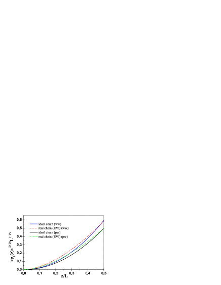
Figure 1: The dimensionless value of the layer monomer density $<\rho_{\lambda}(z)>L^{1-1/\nu}$ profiles for: ideal and real polymer chains in the case of two repulsive walls (D-D b.c)(ww) with $y=10$, and dilute polymer solution ($R_{x}=0.1\mu m$) of ideal and real polymer chains in semi-infinite space containing repulsive spherical particle of big radius $R=10.0\mu m$ on the distance $a=1.0\mu m$ from the repulsive wall ($a=L$) (pw). The maximum is at $L/2$.

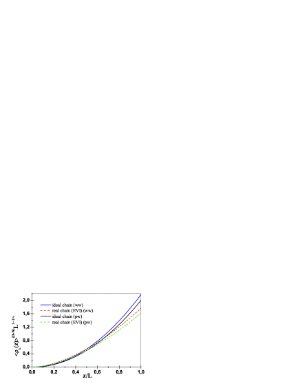
Figure 2: The dimensionless value of the layer monomer density $<\rho_{\lambda}(z)>L^{1-1/\nu}$ profiles for: ideal and real polymer chains in the case of one repulsive one inert wall (D-N b.c.) (ww) with $y=10$, and dilute polymer solution ($R_{x}=0.1\mu m$) of ideal and real polymer chains in semi-infinite space containing inert spherical particle of big radius $R=10.0\mu m$ on the distance $a=1.0\mu m$ from the repulsive wall ($a=L$) (pw). The maximum is near the distant inert wall.

In order to test the reliability of the obtained analytical results it will be interesting to compare them with the recent results of Monte Carlo calculations obtained by HG04 for the single polymer chain trapped inside the slit of two repulsive walls.

In Ref. HG04 the lattice Monte Carlo algorithm on a regular cubic lattice in $d=3$ dimensions, with $D$ lattice units in $z$-direction and impenetrable boundaries was applied ($L=uD$ with $u$ denoting the lattice spacing). The other directions obeyed periodic boundary conditions. The correspondent reduced force in accordance with (HG04 ) can be written in the form:

$$\frac{f}{k_{B}\,T}\,=\,\frac{{\tilde{a}}}{\nu\,\mu_{\infty}L}\,\sqrt{3}^{\frac{1}{\nu}}\,\left(\frac{L}{R_{x}}\right)^{-\frac{1}{\nu}},$$ (20)

where parameter ${\tilde{a}}$ is a universal amplitude, $\mu_{\infty}$ is the critical fugacity per monomer. Taking into account Eq.(10) and the value $B_{ideal}$ from (13), the monomer density near the wall for ordinary RW is scaled as:

$$<\rho_{\lambda}(z)>_{G}=\frac{2\pi^{2}z^{2}}{L}\left(\frac{L}{R_{x}}\right)^{-2},$$ (21)

where the universal amplitude ${\tilde{a}}$ for the case of ideal chains was found as ${\tilde{a}}\approx 0.2741(2)$ (see Ref.HG04 ), which is very close to the exact value, computed analytically in E97 and equal to ${\tilde{a}}=\frac{\pi^{2}}{36}$. For the ideal chain takes place: $\nu=0.5$, $\chi_{d}=1$ and $\mu_{\infty}=\frac{1}{6}$. In Fig.3 this asymptotic behaviour for narrow slits is clearly recovered by our results for ideal chains, where the narrow slit limit is valid.

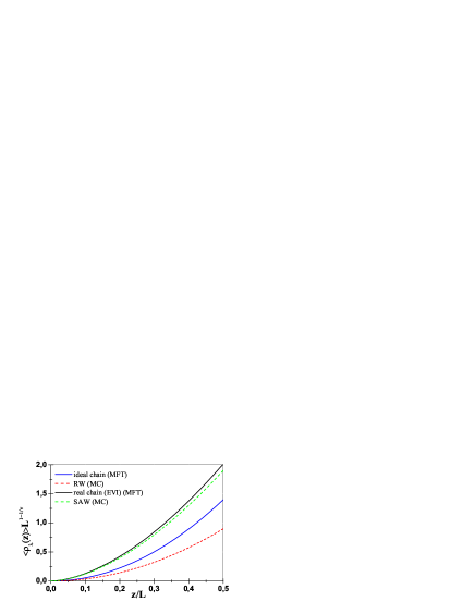
Figure 3: Comparison of theoretical results with Monte Carlo simulations for the layer monomer density $<\rho_{\lambda}(z)>$ profiles for: ideal chain and real polymer chain with EVI (MFT) in the case of two repulsive walls (D-D b.c). RW(MC) and SAW(MC) are the results obtained in Ref.HG04 for random walks and self avoiding walks. The comparison of results are performed for the case: $D=80$, $N=3500$ and $y\approx 2.34$ (RW); $D=120$, $N=3500$ and $y\approx 1.73$ (SAW) .

In the case of SAW in Ref. HG04 the value ${\tilde{a}}\approx 0.448\pm 0.005$ was obtained. Taking into account the values for $\nu\approx 0.588$, $\chi_{3}^{2}\approx 0.960$ (e.g. CJ90 ) and $\mu_{\infty}\approx 0.2135$, $B_{real}=1.70\pm 0.08$ (see Ref. HG04 ), the correspondent monomer density for SAW can be written as

$$<\rho_{\lambda}(z)>_{EVI}\,\approx\,\frac{15.44\,z^{1.7}}{L}\left(\frac{L}{R_{x}}\right)^{-1.7}\,\,.$$ (22)

The result Eq.(22) is presented in Fig.3 and compared to our theoretical results for a trapped chain with EVI, which are valid for the wide slit regime $y\gtrsim 1$. In order to compare the obtained analytical results with recent results of MC simulation we performed extrapolation of the MC results for ${\tilde{a}}$ and $\mu_{\infty}$ which are valid for the narrow slit regime to the region of $y\gtrsim 1$. As it possible to see from Fig.3, the results Eq.(21) and Eq.(22) correspond very well to our theoretical predictions in the wide slit limit. One of the possible reasons for remaining deviations with the results of Ref. HG04 is that the chain in the MC simulation is too short in order to compare with the results of the field-theoretical RG group approach. Unfortunately, at the moment no simulations concerning one repulsive and one inert wall exist.

References

- (1) J.F.Joanny, L.Leibler, and P.G. de Gennes, J.Polym.Sci., Polym.Phys.Ed. 17, 1073 (1979).
- (2) E.Eisenriegler, Phys.Rev.E 55, 3116 (1997).
- (3) A.Milchev and K.Binder, Eur.Phys.J.B 3, 477 (1998); 13, 607 (2000).
- (4) H.-P.Hsu and P.Grasberger, J.Chem.Phys. 120, 2034 (2004).
- (5) G.Parisi, J.Stat.Phys. 23, 49 (1980).
- (6) G.Parisi, Statistical Field Theory (Addison-Wesley, Redwood City, 1988).
- (7) H.W.Diehl, M.Shpot, Nucl. Phys. B 528, 595 (1998).
- (8) Z.Usatenko, J.Stat.Mech., P03009 (2006).
- (9) D.Romeis, Z.Usatenko, Phys.Rev.E 80, 041802 (2009).
- (10) P.G. de Gennes, Phys.Lett.A 38, 339 (1972); Scaling Concepts in Polymer Physics (Cornell University Press, Ithaca, NY, 1979).
- (11) H.W.Diehl and S.Dietrich, Z.Phys.B 42, 65 (1981).
- (12) J.L.Cardy, Phys.Rev.Lett. 65, 1443 (1990).
- (13) E.Eisenriegler, Polymers Near Surfaces (World Scientific Publishing Co.Pte.Ltd., Singapore, 1993).
- (14) E.Eisenriegler, M.Krech, and S.Dietrich, Phys.Rev.B 53, 14377 (1996).
- (15) H.W.Diehl, S.Dietrich, and E.Eisenriegler, Phys.Rev.B 27, 2937 (1983).
- (16) H. W. Diehl, in Phase Transitions and Critical Phenomena, edited by C. Domb and J. L. Lebowitz (Academic Press, London, 1986), Vol. 10, pp. 75–267.
- (17) Z.Usatenko, J.Chem.Phys. 133, 2010 (in press).
- (18) B.V.Derjaguin, Kolloid-Z. 69, 155 (1934).
- (19) J.des Cloizeaux and G.Jannink, Polymers in Solution (Clarendon Press, Oxford, 1990).