Numerical Estimation of the Current Large Deviation Function in the Asymmetric Simple Exclusion Process with Open Boundary Conditions

Abstract

We numerically study the large deviation function of the total current, which is the sum of local currents over all bonds, for the symmetric and asymmetric simple exclusion processes with open boundary conditions. We estimate the generating function by calculating the largest eigenvalue of the modified transition matrix and by population Monte Carlo simulation. As a result, we find a number of interesting behaviors not observed in the exactly solvable cases studied previously as follows. The even and odd parts of the generating function show different system-size dependences. Different definitions of the current lead to the same generating function in small systems. The use of the total current is important in the Monte Carlo estimation. Moreover, a cusp appears in the large deviation function for the asymmetric simple exclusion process. We also discuss the convergence property of the population Monte Carlo simulation and find that in a certain parameter region, the convergence is very slow and the gap between the largest and second largest eigenvalues of the modified transition matrix rapidly tends to vanish with the system size.

1 Introduction

Current, such as electric current, heat flow, or current of matter, plays important roles in nonequilibrium systems. The presence of macroscopic current is a signature of nonequilibrium states. Near equilibrium, the current is proportional to the conjugate external field and the linear coefficient is given by the autocorrelation function of the current in equilibrium states[1]. Beyond the linear regime, although we do not know much about general properties of the current in strongly interacting systems, current fluctuations are considered as key quantities to understand the dynamical behavior of nonequilibrium systems. In this respect, the large deviation property of the current is being studied intensively[2, 3, 4] in various systems. The large deviation function characterizes the probability of the time-integrated current in the long-time limit and its Legendre transform gives the cumulant generating function. Thus, it contains information about not only the mean and the variance but also higher-order cumulants, which are related to the nonlinear transport coefficients in the full counting statistics[5]. In the context of statistical physics, the time-integrated current called the Helfand moment is related to the Green-Kubo formula[6]. The shear viscosity and the thermal conductivity calculated with the Helfand moment in the recent simulations are in excellent agreement with those calculated with the Green-Kubo formula[7, 8]. It is also suggested that the current large deviation is relevant to understanding the dynamical behavior of glasses[9].

The simple exclusion process (SEP) is probably the simplest and best studied model of nonequilibrium systems[10, 11]. The SEP is defined on the one-dimensional lattice, where particles are allowed to move to one of the nearest neighbor sites when the site to move to is empty. If the leftward and rightward hopping rates are the same, the model is called the symmetric simple exclusion process (SSEP). If the hopping rates are different, the model is called the asymmetric simple exclusion process (ASEP). Two extreme cases of the ASEP have special names. When the difference is as small as the inverse of the system size, the model is referred to as the weakly ASEP (WASEP). The totally ASEP (TASEP) means that one of the hopping rates becomes zero. The ASEP is applied to various phenomena such as traffic flow[12], molecular motor transportation[13], the process of copying messenger RNA[14], and sequence alignment[15]. The ASEP in the infinite system with a step initial condition can be mapped to a model of surface growth, and recent experiments show that the height fluctuations of the growing surface in electroconvection, which correspond to the current fluctuations in the ASEP, obey the Tracy-Widom distribution function[16] that appear in the exact solution of the one-dimensional Karar-Parisi-Zhang equation[17].

For the ASEP with open boundary conditions, the stationary state is exactly calculated with the matrix product method[18, 19, 20] or with the recursion relation[21]. In particular, it is clarified that the system has three phases, the low-density phase, the high-density phase, and the maximum-current phase, depending on the particle’s entering and exiting rates at the boundaries. The transition between the maximum-current phase and the other phases is second order and that between the low-density and high-density phases is first order. Thus, in the latter case, the two phases can coexist on the phase transition line, where a kink appears between the low-density region and the high-density region. The random walk motion of the kink contributes to the power-law behavior of the power spectrum[22, 23].

The current large deviation functions for the SSEP with the open boundary condition were studied by Derrida et al.[24, 3], who obtained the scaling form for the generating function. The TASEP[25, 26] and the WASEP[27] on a ring, and the SSEP in the infinite system with the step initial condition[28] were studied by applying the Bethe ansatz. The direct calculation of the probability of the number of particles passing through a certain site was performed on the TASEP and the WASEP in the infinite system with some special initial conditions,[29, 30] and it turned out that different initial conditions lead to different types of scaling behavior. The current moments of the ASEP in the infinitely large system have recently been studied by Imamura and Sasamoto[31], who showed that the calculation of the $n$th moment is reduced to the problem of the ASEP with a system with particles less than or equal to $n$. The macroscopic fluctuation theory has been developed as a theory for the large deviation function[32, 33, 34, 35]. It is based on the postulate that the large deviation function is characterized only by the mean and variance of the current. The macroscopic fluctuation theory is applied to the SSEP[36] and the WASEP[34]. In the ASEP, the joint probability of the current and the density is calculated for some restricted boundary conditions by using the matrix product method[37]. For the current through the boundary, the generating function in the ASEP with open boundary conditions where both input and output are allowed at each boundary is calculated by using the Bethe ansatz[38] for the low- and high- density phases, and the symmetry relation for the current is also discussed[39].

In addition to the exact calculations, many numerical studies have been carried out. A population Monte Carlo method[40] was devised to calculate the large deviation functions first for discrete time dynamics[41], and it was extended to continuous time[42]. By using these methods, the large deviation functions in the zero range process[43] and in the Kipnis-Marchioro-Pressuti (KMP) model[44], which is a simple model of heat conduction, were computed. The density matrix renormalization group (DMRG) method was also applied to obtain the current large deviation for the TASEP with open boundary conditions[45].

Despite these extensive studies and the importance of the applications, the current large deviation function in the ASEP with open boundary conditions has not yet been fully understood. Furthermore, the definition of the current varies in the studies. Some studies consider the current through a bond and other studies consider the total current, which is the sum of the former over all bonds. Although the averages of these two quantities are trivially equivalent, their fluctuations may behave differently.

In the present study, we numerically calculate the current large deviation function in the SEP with open boundary conditions and find several properties that have not been reported in the exactly solvable cases. The large deviation function shows a cusp near zero current when the asymmetry is large. In both the SSEP and the ASEP, the even part of the generating function depends linearly on the system size, while the odd part does not. Our finding indicating that the even-order cumulants are proportional to system size $L$ differs from that obtained in the preceding study,[36] where the $n$th-order cumulant is proportional to $L^{n-1}$. We compare the generating functions for the two definitions of the current and find that they coincide with each other in the direct evaluation using the largest eigenvalue method, while the population Monte Carlo method fails when the current through a boundary is employed. Thus, the use of the total current has an advantage in the Monte Carlo simulation. We estimate numerical errors in the Monte Carlo simulation using the symmetry relation and find that the deviation is usually small. However, the Monte Carlo simulation sometimes shows an unexpectedly slow convergence and produces no reliable results. In those cases, the difference between the largest and second largest eigenvalues of the modified Master equation decays faster than the exponential of the system size.

This paper is organized as follows. In $\S$2, we give a brief review for the SEP and the current large deviation function, and explain two numerical methods that we use in the present simulations involving the use of the largest eigenvalue of the modified Master equation and the population Monte Carlo method. We also give a short summary of the studies of the current large deviation for the SSEP and the ASEP under open boundary conditions. In the next section, we show our numerical results. In particular, we focus on the difference induced by different definitions of current. The convergence problem in the population Monte Carlo method is also discussed. The last section is devoted to discussion and conclusions.

2 Model and Algorithm

2.1 ASEP and Master equation

The SEP is a continuous-time Markov process defined on a one-dimensional chain. We denote $\tau_{j}=1$ if site $j$ is occupied by a particle and $\tau_{j}=0$ if the site $j$ is empty. The configuration of the system of size $L$ is described by the set $C=\{\tau_{1},\tau_{2},\dots,\tau_{L}\}$. A particle can hop to the left or right nearest-neighbor site if the destination site is empty. Namely, the particles are subject to the exclusion interaction. The hopping rate to the right is denoted by $p_{r}$ and that to the left by $p_{l}$. If site 1 is empty, a particle enters with rate $\alpha$, and if the site is occupied, the particle exits with rate $\gamma$. Similarly, if site $L$ is empty, a particle enters with rate $\delta$, and if the site is occupied, the particle exits with rate $\beta$.

Let us denote the probability for the system to be in configuration $C$ at time $t$ by $P(C,t)$. By using the transition rate from the configuration $C^{\prime}=\{\tau^{\prime}_{1},\dots,\tau^{\prime}_{L}\}$ to $C=\{\tau_{1},\dots,\tau_{L}\}$, $W_{CC^{\prime}}$, the time evolution of $P(C,t)$ is described by the Master equation

$$\frac{{\rm d}}{{\rm d}t}P(C,t)=\sum_{C^{\prime}(\neq C)}\left[W_{CC^{\prime}}P(C^{\prime},t)-W_{C^{\prime}C}P(C,t)\right].$$ (1)

In the ASEP, the transition rate is written as

$$W_{CC^{\prime}} = w_{1}\delta_{\tau_{2}\tau^{\prime}_{2}}\cdots\delta_{\tau_{L}\tau^{\prime}_{L}}$$ (2)

$$+\delta_{\tau_{1}\tau^{\prime}_{1}}\cdots\delta_{\tau_{j-1}\tau^{\prime}_{j-1}}\sum_{j=1}^{L-1}w_{j,j+1}\delta_{\tau_{j+2}\tau^{\prime}_{j+2}}\cdots\delta_{\tau_{L}\tau^{\prime}_{L}}$$

$$+\delta_{\tau_{1}\tau^{\prime}_{1}}\cdots\delta_{\tau_{L-1}\tau^{\prime}_{L-1}}w_{L},$$

where $\delta_{\tau_{i}\tau^{\prime}_{i}}=(1-\tau_{i})(1-\tau^{\prime}_{i})+\tau_{i}\tau^{\prime}_{i}$,

$$w_{1}=\alpha(1-\tau^{\prime}_{1})\tau_{1}+\gamma\tau^{\prime}_{1}(1-\tau_{1}),$$ (3)

$$w_{L}=\delta(1-\tau^{\prime}_{L})\tau_{L}+\beta\tau^{\prime}_{L}(1-\tau_{L}),$$ (4)

and

$$w_{j,j+1}=p_{r}\tau^{\prime}_{j}(1-\tau^{\prime}_{j+1})(1-\tau_{j})\tau_{j+1}$$ (5)

$$+p_{l}(1-\tau^{\prime}_{j})\tau^{\prime}_{j+1}\tau_{j}(1-\tau_{j+1}).$$

If we denote $r(C)=\sum_{C^{\prime}(\neq C)}W_{C^{\prime}C}$, eq. (1) is rewritten as

$$\frac{{\rm d}}{{\rm d}t}P(C,t)=\sum_{C^{\prime}(\neq C)}W_{CC^{\prime}}P(C^{\prime},t)-r(C)P(C,t).$$ (6)

Thus, $r(C)$ means the rate of transition from $C$ to any other configurations.

The time evolution of the system is decomposed into the set of one-particle movements that we call a path. Consider that the system starts with initial configuration $C_{0}$ at time $t_{0}$. The configuration changes from $C_{i-1}$ to $C_{i}$ when a particle changes its position or a particle enters or exits from the system at time $t_{i}$ ($i=1,\dots,K$), reaches $C_{K}$ at $t_{K}$, and remains in the same state until time $t$. Thus, the state at time $t$ is $C=C_{K}$. This path is represented as $(C,t;C_{K},t_{K};\dots;C_{1},t_{1}|C_{0},t_{0})$. Now, we denote the probability that the transition from $C_{i-1}$ to $C_{i}$ occurs between time $t_{i}$ and $t_{i}+{\rm d}t_{i}$ for $i=1,2,\dots,K$ by

$$P(C,t;C_{K},t_{K};\dots;C_{1},t_{1}|C_{0},t_{0}){\rm d}t_{K}\dots\rm dt_{2}{\rm d}t_{1}.$$ (7)

Then the path probability density $P(C,t;C_{K},t_{K};\dots;C_{1},t_{1}|C_{0},t_{0})$ for $K\geq 1$ is written as

$$P(C,t;C_{K},t_{K};\dots;C_{1},t_{1}|C_{0},t_{0})$$ (8)

$$= \delta_{CC_{K}}e^{-r(C_{K})(t-t_{K})}W_{C_{K}C_{K-1}}$$

$$\cdots e^{-r(C_{1})(t_{2}-t_{1})}W_{C_{1}C_{0}}e^{-r(C_{0})(t_{1}-t_{0})}$$

$$= \delta_{CC_{K}}\exp\left[-\sum_{i=0}^{K}r(C_{i})(t_{i+1}-t_{i})\right]\prod_{j=0}^{K-1}W_{C_{j+1}C_{j}},$$

where $t_{K+1}$ should be understood as $t$. Because $K$ represents the number of one-particle movements, if $K=0$, $P(C,t;C_{K},t_{K};\dots;C_{1},t_{1}|C_{0},t_{0})$ should be interpreted as representing the probability that no transitions occur at the time interval $[t_{0},t]$, which equals $\delta_{CC_{0}}e^{-r(C_{0})(t-t_{0})}$. The relationship between the conditional probability $P(C,t|C_{0},t_{0})$ and the path probability density is given by

$$P(C,t|C_{0},t_{0})$$ (9)

$$= \sum_{K=0}^{\infty}\sum_{C_{1},C_{2},\dots,C_{K}}\int_{t_{0}}^{t}{\rm d}t_{K}\int_{t_{0}}^{t_{K}}{\rm d}t_{K-1}\cdots\int_{t_{0}}^{t_{2}}{\rm d}t_{1}$$

$$P(C,t;C_{K},t_{K};\dots;C_{1},t_{1}|C_{0},t_{0}).$$

If we differentiate the above equation with respect to $t$, we reobtain the Master equation.

2.2 Large deviation function and generating function

Let us denote the probability that the mean current takes the value $q$ as

$$q=\frac{1}{t}\sum_{i=0}^{K-1}Q(C_{i+1},C_{i})$$ (10)

by $P(q)$. The microscopic current $Q(C_{i+1},C_{i})$ takes the value $1(-1)$ when the particle moves forward (backward) during the configuration change from $C_{i}$ to $C_{i+1}$. A precise definition of the microscopic current is given in the next subsection. When $t$ is large, this probability asymptotically behaves as

$$P(q)\simeq e^{-tf(q)},$$ (11)

where $f(q)$ is called the large deviation function. As a result of the law of large number, $f(q)$ must have a minimum at a certain value $q^{*}$ and satisfy $f(q^{*})=0$. The Legendre transform of $f(q)$ is called the generating function, which we write

$$\mu(\lambda)=\max_{q}\left[\lambda q-f(q)\right].$$ (12)

The generating function satisfies $\mu(0)=0$ that corresponds to $f(q^{*})=0$. Similarly, the large deviation function is given by the Legendre transform of the generating function as

$$f(q)=\max_{\lambda}\left[q\lambda-\mu(\lambda)\right].$$ (13)

The generating function is also rewritten as

$$e^{\mu(\lambda)t}=\langle e^{\lambda qt}\rangle$$ (14)

for large $t$. This means that the generating function is expanded as

$$\mu(\lambda)=\sum_{n=1}^{\infty}\frac{1}{n!}\mu^{(n)}(0)\lambda^{n}=\sum_{n=1}^{\infty}\frac{1}{n!}\langle q^{n}\rangle_{c}t^{n-1}\lambda^{n}$$ (15)

with respect to the cumulants $\langle q^{n}\rangle_{c}$, or the cumulants are generated as

$$\langle q^{n}\rangle_{c}=\frac{1}{t^{n-1}}\left.\frac{\partial^{n}\mu(\lambda)}{\partial\lambda^{n}}\right|_{\lambda=0},$$ (16)

which is the origin of the name of the function.

The expectation in the rhs of eq. (14) is taken with respect to the path probability. Thus, we obtain

$$\langle e^{\lambda qt}\rangle=\sum_{K=0}^{\infty}\sum_{C_{K},\cdots,C_{1},C}\int_{t_{0}}^{t}{\rm d}t_{K}\int_{t_{0}}^{t_{K}}{\rm d}t_{K-1}\cdots\int_{t_{0}}^{t_{2}}{\rm d}t_{1}$$ (17)

$$\delta_{C_{K}C}e^{\lambda\sum_{i=0}^{K-1}Q(C_{i+1},C_{i})}e^{-r(C_{K})(t-t_{K})}$$

$$\prod_{i=0}^{K-1}W_{C_{i+1}C_{i}}e^{-r(C_{i})(t_{i+1}-t_{i})}.$$

If we introduce $W^{\lambda}_{CC^{\prime}}=W_{CC^{\prime}}e^{\lambda Q(C,C^{\prime})}$ and

$$P^{\lambda}(C,t|C_{0},t_{0})$$ (18)

$$= \sum_{K=0}^{\infty}\sum_{C_{K},\cdots,C_{1}}\int_{t_{0}}^{t}{\rm d}t_{K}\int_{t_{0}}^{t_{K}}{\rm d}t_{K-1}\cdots\int_{t_{0}}^{t_{2}}{\rm d}t_{1}$$

$$\delta_{C_{K}C}e^{-\sum_{i=1}^{K}r(C_{i})(t_{i+1}-t_{i})}\prod_{j=0}^{K-1}W^{\lambda}_{C_{j+1}C_{j}},$$

the generating function is obtained as

$$\mu(\lambda)=\lim_{t\to\infty}\frac{1}{t}\log\left[\sum_{C}P^{\lambda}(C,t|C_{0},t_{0})\right],$$ (19)

or we may assume some initial distribution $P_{0}(C_{0})$ and substitute

$$P^{\lambda}(C,t)=\sum_{C_{0}}P^{\lambda}(C,t|C_{0},t_{0})P_{0}(C_{0})$$ (20)

in place of $P^{\lambda}(C,t|C_{0},t_{0})$ in the rhs of eq. (19). The time evolution of $P^{\lambda}(C,t)$ obeys the modified master equation

$$\frac{{\rm d}}{{\rm d}t}P^{\lambda}(C,t)=\sum_{C^{\prime}\neq C}W^{\lambda}_{CC^{\prime}}P^{\lambda}(C^{\prime},t)-r(C)P^{\lambda}(C,t).$$ (21)

We note here that because $\sum_{C^{\prime}(\neq C)}W^{\lambda}_{CC^{\prime}}\neq r(C)$, this equation cannot be interpreted as an evolution of probability. Namely, $\sum_{C}P^{\lambda}(C,t)$ varies in time. In the vector form, eq. (21) is written as

$$\frac{\rm d}{{\rm d}t}\mathsf{P}^{\lambda}(t)=\mathsf{W}^{\lambda}\mathsf{P}(t),$$ (22)

where $\mathsf{P}^{\lambda}(t)$ is the vector whose $C$th element is $P^{\lambda}(C,t)$, and the $\lambda$-modified transition matrix $\mathsf{W}^{\lambda}$ is defined as

$$\left(\mathsf{W}^{\lambda}\right)_{CC^{\prime}} = \left\{\begin{array}[]{l}W^{\lambda}_{CC^{\prime}}\;\mbox{for}\;C\neq C^{\prime}\\ -r(C)\;\mbox{for}\;C=C^{\prime}\end{array}\right..$$ (25)

Because eq. (21) is linear, the solution is spectrally decomposed into

$$P^{\lambda}(C,t)=\sum_{n}e^{\zeta_{n}t}\psi_{n}(C)\sum_{C^{\prime}}\psi^{\prime}_{n}(C^{\prime})P_{0}(C^{\prime}),$$ (26)

where $\zeta_{n}$ is the eigenvalue and $\psi^{\prime}_{n}(C)$ and $\psi_{n}(C)$ are the corresponding left and right eigenvectors of $\mathsf{W}^{\lambda}$. In the long time limit, only the term with the largest eigenvalue $\zeta_{\mathrm{max}}$ is dominant, and accordingly the generating function becomes equal to $\zeta_{\mathrm{max}}$. Thus, we can estimate the generating function by numerically calculating the largest eigenvalue of the $\lambda$-modified transition matrix if exact calculations are not possible. This method is powerful but restricted to small systems because of memory limitations.

2.3 Definition of the microscopic current

There are two different definitions of current. One is the current through the boundary of the system. From the equation of continuity, this current determines changes of the amount of the conserved quantity in the system. The other is the total current given as the spatial integration of the current density. It is natural to use the total current in the linear response theory when we consider the response to a static and uniform external field or thermal force.

Both definitions appear in the literature of SEP. In the studies of current large deviations of the SEP with periodic boundaries, the total current is employed by Derrida and Lebowitz[25], Derrida and Appert,[26] and Prolhac and Mallick[27]. On the contrary, the current through the left boundary is used by Derrida et al. [24, 3] or de Gier and Essler[39, 38], who study the systems with open boundaries.

We let $Q_{A}$ denote the total current defined as

$$Q_{A}(C_{i+1},C_{i}) = \sum_{j=1}^{L-1}\left[-\tau^{i}_{j}(1-\tau^{i}_{j+1})(1-\tau^{i+1}_{j})\tau^{i+1}_{j+1}\right.$$ (27)

$$\mbox{}\left.+(1-\tau^{i}_{j})\tau^{i}_{j+1}\tau^{i+1}_{j}(1-\tau^{i+1}_{j+1})\right]$$

$$\mbox{}-(1-\tau^{i}_{1})\tau^{i+1}_{1}+\tau^{i}_{1}(1-\tau^{i+1}_{1})$$

$$+(1-\tau^{i}_{L})\tau^{i+1}_{L}-\tau^{i}_{L}(1-\tau^{i+1}_{L}),$$

and $Q_{B}$ denote the current through the left boundary as

$$Q_{B}(C_{i+1},C_{i}) = -(1-\tau^{i}_{1})\tau^{i+1}_{1}+\tau^{i}_{1}(1-\tau^{i+1}_{1}).$$ (28)

For each current, we define the mean current $q_{X}$ ($X=A$ or $B$) as

$$q_{X}=\frac{1}{t}\sum_{i=0}^{K-1}Q_{X}(C_{i+1},C_{i}),$$ (29)

and the generating function $\mu_{X}(\lambda)$ as

$$e^{\mu_{X}(\lambda)}=\langle e^{\lambda q_{X}t}\rangle.$$ (30)

We note that the positive direction of the currents (27) and (28) is defined as leftward in this paper. We use the character $q$ for a current if we do not need to specify $q_{A}$ or $q_{B}$, or for a current in general. Since the system goes to a stationary state in the long-time limit, we obtain

$$\langle q_{A}\rangle=(L+1)\langle q_{B}\rangle.$$ (31)

Thus, the two definitions are equivalent with respect to expectation values except the trivial factor.

Our question here is whether the large deviation properties of the two currents appear the same or not. Theoretically, they are considered equivalent as follows[46]. If a path is fixed, most particles that enter the system through a boundary exit from either boundary and the contribution from such particles to $q_{A}$ is exactly $L+1$ times the contribution to $q_{B}$. The number of such particles is proportional to $t$. On the contrary, the particles initially present in the system or those remaining in the system at time $t$ contribute to $q_{A}$ and $q_{B}$ differently. However, the number of those particles should be $t$-independent and the contribution from those particles is negligible for a large time. Thus, $q_{A}$ and $q_{B}$ are supposed to be essentially the same. Despite such consideration, how they appear in the numerical experiment is a different problem. Actually, as will be clarified later, the use of the total current has an advantage in the Monte Carlo simulations.

2.4 Monte Carlo simulations

If the system size is so large that the direct evaluation of the largest eigenvalue is not possible, we can employ a Monte Carlo method. However, because $P_{\lambda}(C,t)$ is not a probability distribution function, conventional Monte Carlo methods cannot be used. In fact, an algorithm based on the diffusion Monte Carlo method is devised by Giardinà et al.[41] and extended to a continuous-time case by Lecomte and Tailleur[42]. In those algorithms, besides the conventional Monte Carlo dynamics, we introduce clones of configuration $C$. The clones are duplicated or pruned with the rate $y(C)=e^{(r_{\lambda}(C)-r(C))\Delta t}$, where $\Delta t$ is the Poisson-distributed waiting time and its distribution function is given as

$$r_{\lambda}(C)e^{-r_{\lambda}(C)\Delta t},$$ (32)

where

$$r_{\lambda}(C)=\sum_{C^{\prime}\neq C}W^{\lambda}_{CC^{\prime}}.$$ (33)

Thus, the mean waiting time is $1/r_{\lambda}(C)$. Since the number of clones must be limited in the computer, we actually need an additional algorithm to keep the number of clones constant. If the clone is to be pruned, we choose a random clone and copy over the pruned one, and if the clone is to be duplicated, we copy the clone on the randomly chosen clone.

The precise algorithm is as follows.

1. Set initial conditions for $N$ clones.

2. Choose which clone to evolve. Here, we name it $c^{\alpha}$. First, the clones are chosen orderly. After all the clones evolve in the initial step, the clone with the earliest time is chosen.

3. Calculate the transition probability $W^{\lambda}_{CC^{\prime}}/r_{\lambda}(C)$, and let a transition take place. The time interval $\Delta t$ is chosen from the Poisson law.

4. Calculate $y(C)$ and set $y=[y(C)+\xi]$, where $\xi$ is a uniform random number in $0\leq\xi<1$ and $[x]$ is the integer part of $x$. If $y=1$, the clone $c^{\alpha}$ is preserved; if $y=0$, the clone $c^{\alpha}$ is erased and overwritten by another randomly chosen clone; and if $y>1$, $y-1$ clones are chosen randomly and overwritten with the clone $c^{\alpha}$.

Thus, the total number of clones is kept constant. We denote $y$ at the $i$th time step by $y_{i}$ and define $X_{i}=(N+y_{i}-1)/N$. Thus, the generating function is given by the following formula in the long-time limit:[42]

$$\mu(\lambda)=\frac{1}{t}\ln(X_{1}\cdots X_{K}),$$ (34)

where $K$ is the number of state changes.

Lecomte and Tailleur[42] introduced another method called thermodynamic integration. Because the generating function is written as

$$\mu(\lambda)=\frac{1}{t}\ln\langle e^{q\lambda t}\rangle,$$ (35)

its derivative is

$$\mu^{\prime}(\lambda)=\frac{\langle qe^{q\lambda t}\rangle}{\langle e^{q\lambda t}\rangle}=\bar{q}^{\lambda},$$ (36)

which can be interpreted as the average value of $q$ with respect to the population of clones. Thus, obtaining $\bar{q}^{\lambda}$ numerically and integrating it from $0$ to $\lambda$, we obtain

$$\mu(\lambda)=\int_{0}^{\lambda}{\rm d}\lambda^{\prime}\bar{q}^{\lambda^{\prime}}.$$ (37)

This thermodynamic integration gives a smoother result than the direct evaluation (34). In this study, we use both methods and adopt a better result.

2.5 Known results and the symmetry relations

There are some known results about the current large deviation for the SEP with open boundaries.

The cumulants of the current in the SSEP were calculated [36] under the conjecture of the additivity principle as

$$\langle q_{b}\rangle = \frac{I_{1}}{L}$$ (38)

$$\langle q_{b}^{2}\rangle_{c} = \frac{tI_{2}}{LI_{1}}$$ (39)

$$\langle q_{b}^{3}\rangle_{c} = \frac{t^{2}}{L}\frac{3(I_{3}I_{1}-I_{2}^{2})}{I_{1}^{3}}$$ (40)

$$\langle q_{b}^{4}\rangle_{c} = \frac{t^{3}}{L}\frac{3(5I_{4}I_{1}^{2}-14I_{1}I_{2}I_{3}+9I_{2}^{3})}{I_{1}^{5}}$$ (41)

$$I_{n} = \int_{\rho_{b}}^{\rho_{a}}{\rm d}\rho D(\rho)\sigma(\rho)^{n-1}.$$ (42)

Here, the macroscopic parameters are $D(\rho)=1$ and $\sigma(\rho)=2\rho(1-\rho)$, and the boundary parameters are $\rho_{a}=\frac{\alpha}{\alpha+\gamma}$ and $\rho_{b}=\frac{\delta}{\beta+\delta}$ . Note that all the cumulants are proportional to $1/L$.

Next, a fluctuation-theorem-like symmetry was found for the current large deviation function for the SSEP [24, 3] as

$$f(q_{B})-f(-q_{B})=A_{B}q_{B},$$ (43)

where $A_{B}$ is the constant written as

$$A_{B}=\ln{\frac{\alpha\beta}{\gamma\delta}}.$$ (44)

De Gier and Essler[39] generalized this to the ASEP, where the same equation (43) holds with the coefficient $A_{B}$ given as

$$A_{B}=\ln{\frac{\alpha\beta}{\gamma\delta}}+(L-1)\ln{\frac{p_{l}}{p_{r}}}.$$ (45)

The coefficient $A_{B}$ was derived from the detailed balance condition given by Enaud and Derrida[47], which is of the form

$$\frac{\alpha\beta}{\gamma\delta}\left(\frac{p_{l}}{p_{r}}\right)^{L-1}=1.$$ (46)

In the same manner, we can further extend the symmetry relation for the mean total current $q_{A}$ as

$$f(q_{A})-f(-q_{A})=A_{A}q_{A},$$ (47)

where

$$A_{A}=\frac{1}{L+1}A_{B}.$$ (48)

We briefly review other studies related to our study. The WASEP has been well studied. Bodineau and Derrida [34] assumed the macroscopic fluctuation theory and extended the results on the WASEP to the strong asymmetry limit, where they estimated the boundary effect on the local Gaussian fluctuation. Depken and Stinchcombe[37] calculated the joint probability of the density and the current in the TASEP when $\gamma=\delta=0$. Prolhac and Mallick[27] calculated the cumulants of the current in the WASEP with periodic boundary conditions using the Bethe ansatz.

Now, we see that the large deviation for the total current in the SEP with open boundary conditions has not been well studied.

3 Simulation Results

3.1 Open boundary SSEP

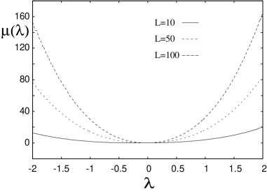
Figure 1: Generating function $\mu_{A}(\lambda)$ calculated by the largest eigenvalue method when $L=10$ and those calculated by the Monte Carlo method when $L=50$ and $100$. The line is interpolated to bring clearness to the graph.

First, we show the results on the open boundary SSEP where the hopping rates are set as $p_{l}=p_{r}=1.0$. Figure 1 shows some examples of the generating function of $q_{A}$ calculated by the two methods; the largest eigenvalue method ($L=10$) and the Monte Carlo method ($L=50$ and $100$). The boundary parameters are chosen as $(\alpha,\beta,\gamma,\delta)=(0.1,0.2,0.9,0.8)$ just for illustration. The generating functions depict parabola-like curves, whose width decreases as the system size increases.

We fit $\mu_{A}(\lambda)$ to the power series up to the sixth order using the least-squares method and examine the system size dependence of the coefficients, which are the cumulants of the current. The fitting is performed in the range $-2\leq\lambda\leq 2$. The first-order cumulant is fixed to the steady current. As seen from Fig. 2, the fitting is successfully performed in the entire range with $L=50$, whereas the fitting up to the second order significantly deviates from the simulation results in the range $|\lambda|\gtrsim 0.5$.

The system size dependence of some low-order cumulants is shown in Fig. 3, where the data of $7\leq L\leq 11$ are obtained from the largest eigenvalues and those of the larger sizes from the Monte Carlo simulations. The boundary parameters are $(\alpha,\beta,\gamma,\delta)=(0.1,0.1,0.1,0.1)$, $(0.1,0.1,0.9,0.9)$, $(0.1,0.3,0.8,0.5)$, and $(0.3,0.3,0.7,0.7)$. In every case, the cumulants of even order are proportional to the system size but those of odd order are not. Thus, the large deviation function cannot be estimated by the mean and the variance only; its characterization needs higher-order statistical quantities. However, we must note that the present fitting is not very reliable, because the result depends on the range of data and on the function to fit with. To obtain more accurate results for the higher-order cumulants, we need a wider range of data. In particular, the cumulants of odd order have relatively small magnitudes and fitting errors are significantly large. Thus, we could not determine how these cumulants really change with the system size.

Figure 2: Comparison between results obtained by the Monte Carlo simulation with $L=50$ and fitting function of the 6th-order. The broken line shows the quadratic part of the 6th-order fitting function.

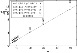
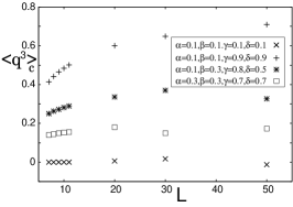
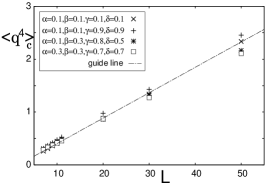
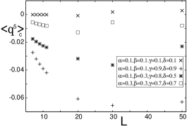
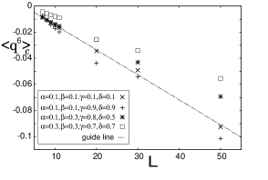
Figure 3: 2nd- through 6th-order cumulants predicted from the fitting of the generating functions given by the simulations. The data of $7\leq L\leq 11$ are given by the largest eigenvalue and the other data are given by the Monte Carlo methods. The data are obtained using the parameters $(\alpha,\beta,\gamma,\delta)=(0.1,0.1,0.1,0.1)$, $(0.1,0.1,0.9,0.9)$, $(0.1,0.3,0.8,0.5)$, and $(0.3,0.3,0.7,0.7)$.

From our results, we conjecture that the generating function split into three parts as

$$\mu_{A}(\lambda)=\langle q_{A}\rangle\lambda+\mu_{A,\mathrm{odd}}(\lambda)+\mu_{A,\mathrm{even}}(\lambda).$$ (49)

The first term in the rhs represents the mean current, which does not depend on the system size for the SSEP and is proportional to the system size for the ASEP. The second term is the even part, which is proportional to the system size $L$. We are not certain how the odd part behaves.

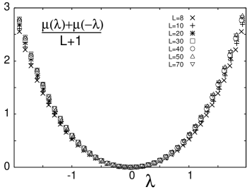
Figure 4: The function $(\mu_{A}(\lambda)+\mu_{A}(-\lambda))/(L+1)$ is plotted with the system sizes of $L=8(\times)$, $10(+)$, $20(\ast)$, $30(\Box)$, $40(\bigcirc)$, $50(\triangle)$, and $60(\triangledown)$.

We show the data of $(\mu_{A}(\lambda)+\mu_{A}(-\lambda))/(L+1)=\frac{2}{L+1}\mu_{A,\mathrm{even}}(\lambda)$ when $L=8$, $10$, $20$, $30$, $40$, $50$, and $70$ in Fig. 4, which shows data collapse. This supports the conjecture that the even part of the generating function is proportional to the system size.

3.2 ASEP with the open boundary conditions

Now, we present the results on the open boundary ASEP, where the transition rates satisfy $p_{l}<p_{r}=1$, and observe whether there are any differences among phases. Because the high-density phase is equivalent to the low-density phase due to the particle-hole symmetry, we examine the remaining two phases (the low-density phase and the maximum-current phase) and the coexisting state of the low- and high-density phases. Figure 5 illustrates the generating function $\mu_{A}(\lambda)$ in each phase of the ASEP with system size $L=10$ and $p_{l}=0.5$. We note that no corresponding analytical or numerical results are indicated in the literature. It is remarkable that any qualitative differences are not observed among the three states.

Figure 5: Generating function $\mu_{A}(\lambda)$ in the ASEP when $L=10$ and $p_{l}=0.5$. Crosses, pluses, and stars correspond to the coexisting phase ($(\alpha,\beta,\gamma,\delta)=(0.1,0.1,0.1,0.1)$), the maximum-current phase ($(0.9,0.9,0.1,0.1)$), and the low-density phase ($(0.1,0.9,0.9,0.1)$), respectively.

As in the SSEP, we have attempted to fit the data with the 6th-order polynomial, and the result for $L=50$, $p_{l}=0.5$, and $(\alpha,\beta,\gamma,\delta)=(0.9,0.9,0.1,0.1)$ is shown in Fig. 6. The fitting seems to work well if a certain neighborhood of the minimum is excluded. We confirmed this property also in other phases. This flattening of the minimum has been reported also in a system with periodic boundary condition[27]. Clearly, the generating function cannot be assumed to be quadratic.

Figure 6: Fitting of the generating function $\mu_{A}(\lambda)$ with 6th-order function in the maximum-current phase. We may fit $\mu_{A}(\lambda)$ well in the region outside the minimum, and this can be seen in other phases.

Similarly to the case of the SSEP, we may divide the generating function for the ASEP into three parts as in eq. (49). We illustrate $(\mu_{A}(\lambda)+\mu_{A}(-\lambda))/(L+1)$ in Fig. 7 for various system sizes $L=8$, $10$, $20$, $30$, and $40$.

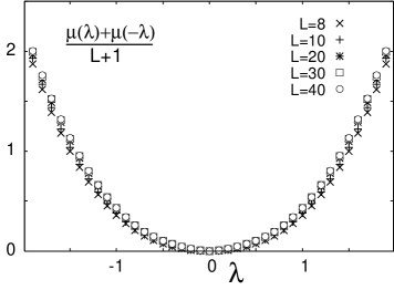
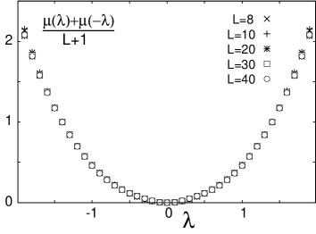
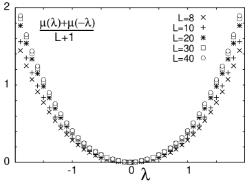
Figure 7: The function $(\mu_{A}(\lambda)+\mu_{A}(-\lambda))/(L+1)$ is plotted with the system sizes of $L=8(\times)$, $10(+)$, $20(\ast)$, $30(\Box)$, and $40(\bigcirc)$, in the low-density phase (top), maximum-current phase (middle) and coexisting phase (bottom).

In relatively small systems, the maximum current phase shows very good data collapse, while the degree of data collapse is not so good in other phases. In every case, however, the data seem to converge in the large-system limit. Thus, as in the SSEP, the even part of the generating function is proportional to the system size when it is sufficiently large.

The large deviation function is obtained from the generating function via the Legendre transformation. Figure 8 shows the plot for $L=10$, $(\alpha,\beta,\gamma,\delta)=(0.1,0.9,0.9,0.1)$, and $p_{l}=0.1,0.2,0.3,0.5$, all of which correspond to the low density phase, in the range $-4\leq q\leq 4$. A blowup near the minimum of $f(q_{A})$ is shown on left of Fig. 8. We note that a cusp appears near $q=0$ and its sharpness increases as $p_{l}$ decreases. This is confirmed by the plot of the derivative of the large deviation function shown on right of Fig. 8. The cusp means that the probability of positive current rapidly decreases with $L$. Such a cusp is seen also in other phases.

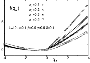
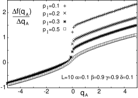
Figure 8: Large deviation function given by the Legendre transform in the range $-5\leq q_{A}\leq 5$. The parameters are $L=10$, $(\alpha,\beta,\gamma,\delta)=(0.1,0.9,0.9,0.1)$ (low-density phase), and $p_{l}=0.1$, $0.2$, $0.3$, and $0.5$. The derivative of the left figure is shown in the right figure.

In the limit $p_{l}\rightarrow 0$, the particles do not move leftward except at the boundaries. Thus, the large deviation function is expected to diverge for $q_{A}>0$ in the limit. This is why the cusp is generated.

3.3 Comparing the two currents

Thus far, we have presented the simulation results for the total currents. In this subsection, we compare the characteristic functions of $q_{A}$ and $q_{B}$. First, we introduce the dimensionless current $q^{N}_{X}$ defined by

$$q^{N}_{X}=\frac{q_{X}}{\langle q_{X}\rangle},$$ (50)

where $\langle q_{X}\rangle$ is the expectation, and then we write the generating function $\mu^{N}_{X}(\lambda)$ of the current $q_{X}^{N}$. We compare $\mu^{N}_{A}(\lambda)$ and $\mu^{N}_{B}(\lambda)$ in the simulations.

The dimensionless current defined here is effective when $\langle q_{X}\rangle$ is known. Fortunately, the steady current is exactly calculated for both the SSEP[48] and the ASEP[20] as

$$\langle q_{B}\rangle_{SSEP}=-\frac{\frac{\delta}{\beta+\delta}-\frac{\alpha}{\gamma+\alpha}}{L+\frac{1}{\alpha+\gamma}+\frac{1}{\beta+\delta}-1},$$ (51)

for the SSEP, and

$$\langle q_{B}\rangle_{ASEP}=\left(\begin{array}[]{cc}(p_{l}-1)\rho_{a}(1-\rho_{a}),&\mbox{low-density and coexisting phases}\\ (p_{l}-1)\rho_{b}(1-\rho_{b}),&\mbox{high-density phase}\\ \frac{p_{l}-1}{4}&\mbox{maximum-current phase}\end{array}\right.$$ (52)

for the ASEP with $p_{l}<p_{r}=1$, where $\rho_{a}$ and $\rho_{b}$ are given as

$$\rho_{a}=\frac{1}{1+a}\qquad a=\frac{1-p_{l}-\alpha+\gamma+\sqrt{(1-p_{l}-\alpha+\gamma)^{2}+4\alpha\gamma}}{2\alpha}$$ (53)

and

$$\rho_{b}=\frac{b}{1+b}\qquad b=\frac{1-p_{l}-\delta+\beta+\sqrt{(1-p_{l}-\delta+\beta)^{2}+4\beta\delta}}{2\beta}.$$ (54)

Henceforth, we omit the suffix ‘SSEP’ or ‘ASEP’ from the steady current $\langle q_{X}\rangle$, for it can be easily understood from the context.

The simulation results from the method of largest eigenvalues are shown in Fig. 9.

Figure 9: Plot of $\mu^{N}_{A}(\lambda)$($\times$) and $\mu^{N}_{B}(\lambda)$($+$) for three sets of parameters. We observe a clear coincidence of $\mu^{N}_{A}(\lambda)$ and $\mu^{N}_{B}(\lambda)$.

It is clear that $\mu^{N}_{A}(\lambda)$ and $\mu^{N}_{B}(\lambda)$ coincide with each other.

However, the two large deviation functions show differences in the Monte Carlo simulation, as shown in Fig. 10. They agree with each other only when $|\lambda|$ is very small and differ greatly outside the region.

Figure 10: Plot of $\mu^{N}_{A}(\lambda)$ and $\mu^{N}_{B}(\lambda)$ for the SSEP and the ASEP. The inset shows the extended plot of the coinciding area.

This difference means that $\mu^{N}_{B}(\lambda)$ is not appropriately calculated in the Monte Carlo simulation. One reason for this is the lack of statistics. Because $q_{B}$ counts only the flux at the left boundary, the number of such events is much smaller than that in the case of $q_{A}$. Another possibility is that the number of clones is not sufficiently large. However, no significant change has been seen in a simulation where we doubled the number of clones and the time duration, as seen in Fig. 11.

Figure 11: Plot of $\mu^{N}_{B}(\lambda)$ for different time step $K$ and clone number $N$ values.

Thus, the difference between the two currents can affect results of the Monte Carlo simulations, though they represent essentially the same physical quantity. The use of the total current $q_{A}$ has an advantage in this respect.

3.4 Symmetry relations

The symmetry relation

$$f(q_{A})-f(-q_{A})=Aq_{A}$$ (55)

should hold in the SEP. First, we show the results for small system sizes obtained from the direct evaluation of the largest eigenvalue. We plot $f(q_{A})-f(-q_{A})$ and $A_{A}q_{A}$ with $A_{A}$ given by eqs. (45) and (48) in Fig. 12. The parameter sets used are $(\alpha,\beta,\gamma,\delta)=(0.1,0.9,0.8,0.2)$ for the low-density phase that we denote by $\times$, $(0.1,0.1,0.1,0.1)$ for the coexisting phase that we denote by $+$, and $(0.9,0.9,0.1,0.1)$ for the maximum-current phase that we denote by $\ast$, and the other parameters $L=10$, $p_{l}=0.5$, and $p_{r}=1.0$ used are the same.

Figure 12: Plot of $f(q_{A})-f(-q_{A})$ from the direct evaluation results represented by $\times,+,$ and $\ast$, and that of $A_{A}q_{A}$ from the analytical result obtained using eq. (48), which is shown by the solid line.

The solid line shows $A_{A}q_{A}$. We see that the symmetric relation is well satisfied in this case.

Next, we consider the results of the Monte Carlo method. In this case, we used the thermodynamic integral to compute the generating function and obtained large deviation functions via the Legendre transform. In Fig. 13 we plot $f(q_{A})-f(-q_{A})$ for the SSEP and the ASEP. The parameter sets are given in the inset of the figure. A negligible deviation is observed for the SSEP, while a small deviation is apparent in the ASEP.

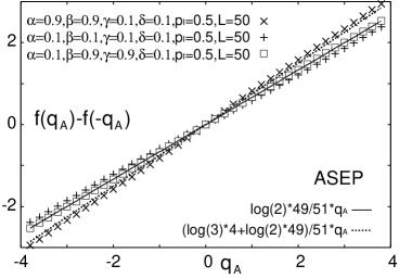
Figure 13: Comparison of $f(q_{A})-f(-q_{A})$ values for the SSEP (top) and ASEP (the others). For the SSEP, the system sizes of $L=30$ and $50$ are plotted. For the ASEP, the plot of $L=30$ is given in the second figure and the plot of $L=50$ is given in the third figure. The parameters are given in the inset. The solid and dotted lines give the analytical results.

The deviation increases with the system size. The error may stem from the insufficient number of clones or the resolution of the data, which affects the precision of the Legendre transform. For large system sizes, the number of necessary clones becomes so large that we could not achieve a higher accuracy. Thus, deviations in Fig. 13 should be interpreted as representing the precision and limitation of the present Monte Carlo simulations.

3.5 Convergence problem in the Monte Carlo method

The Monte Carlo method sometimes presents non-negligible errors. It happens when the hopping asymmetry and the system size are large. For example, Fig. 14 illustrates the instability observed in the numerically obtained generating function. Here, we have chosen the parameters $L=50$, $(\alpha,\beta,\gamma,\delta)=(0.9,0.9,0.1,0.1)$ (maximum-current phase), and $p_{l}=0.2$. This figure shows characteristic fluctuations in the region $0.2<\lambda<1.5$. The true generating function should be a smooth or at least convex function. However, the obtained data does not satisfy the expected convexity.

Figure 14: $\mu(\lambda)$ when $L=50$, $(\alpha,\beta,\gamma,\delta)=(0.9,0.9,0.1,0.1)$ (maximum-current phase), and $p_{l}=0.2$.

To find the cause of the fluctuations, we investigated the initial condition dependence of our Monte Carlo simulation. In Fig. 15, we show how $t^{-1}\ln(X_{1}\cdots X_{K})$ evolves with time in the cases of $\lambda=-1$ and $\lambda=1$ each with three different initial configurations, namely, the empty initial condition (all $\tau_{i}=0$), the random initial condition ($\tau_{i}$ is randomly chosen with probability 1/2), and the half-filled initial condition ($\tau_{i}=1$ for $i<L/2$ and $\tau_{i}=0$ for the other value of $i$). The other parameters used are the same as those indicated in Fig. 14. Note that $\lambda=-1$ corresponds to the stable region and $\lambda=1$ the unstable region. The top of Fig. 15 shows the case $\lambda=-1$, where the three samples exhibit convergence to a common value at $t=10^{4}$. The bottom shows the case $\lambda=1$, where the convergence is very slow and the initial-condition dependence remains even at $t=10^{5}$. This slow convergence is considered to be related to the instability shown in Fig. 14.

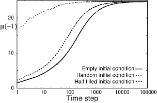
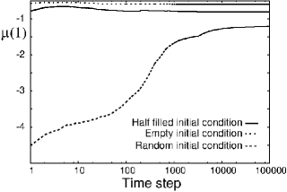
Figure 15: Time evolutions of $\mu(-1)$ (top) and $\mu(1)$ (bottom) when $L=50$ and $p_{l}=0.2$ starting from three initial conditions: empty, random, and half-filled.

The convergence property should be reflected in the spectrum of eigenvalues of the $\lambda$-modified transition matrix $\mathsf{W}^{\lambda}$. Thus, we calculated the second largest eigenvalue $\zeta_{2}$. In Fig. 16, we show the system size dependence of the gap $\zeta_{\mathrm{max}}-\zeta_{2}$ for several $\lambda$ values in the systems of sizes $L=6,\cdots,13$, where $\zeta_{\mathrm{max}}$ is the largest eigenvalue. The top figure shows the cases $\lambda=-0.1$, $0.0$, $0.4$, and $1.6$ on the log-log scale and the bottom figure shows the cases $\lambda=0.0$, $0.1$, $0.16$, $0.2$, and $0.24$ on the semi-log scale.

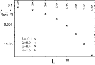
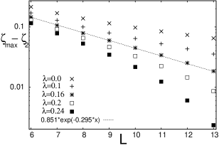
Figure 16: $\zeta_{\mathrm{max}}-\zeta_{2}$ versus the system size $L=6,\cdots,13$. The top figure shows the cases $\lambda=-0.1$, $0.0$, $0.4$, and $1.6$ in the log-log scale and the bottom figure shows the cases $\lambda=0.0$, $0.1$, $0.16$, $0.2$, and $0.24$ in the semi-log scale. The dotted line in the bottom figure is a fitted exponential function.

The figure shows that the magnitude of the gap is proportional to a certain negative power of $L$ in the stable region, whereas the gap decreases faster than the exponential decrease with $L$ in the unstable region. In the bottom of Fig. 16, we see that the system size dependence of $\zeta_{\mathrm{max}}-\zeta_{2}$ changes from the power to exponential and finally to stretched exponential-like. Thus, one reason for the instability of the Monte Carlo calculation found here is considered to be that $\zeta_{2}$ becomes close to $\zeta_{\mathrm{max}}$ as $L$ increases. This behavior suggests that a certain type of phase transition may occur as reported recently[43, 49].

4 Discussion and conclusions

Our simulation results show $\mu_{A}^{N}(\lambda)=\mu_{B}^{N}(\lambda)$, which implies

$$\langle q_{A}^{n}\rangle_{c}\sim L^{n}\langle q_{B}^{n}\rangle_{c}.$$ (56)

From the calculation given by Bodineau and Derrida for the SSEP[24], we may assume $\langle q_{B}^{n}\rangle_{c}\sim\frac{1}{L}$, and thus $\langle q_{A}^{n}\rangle_{c}\sim L^{n-1}$. This relation does not coincide with our result $\langle q_{A}^{2n}\rangle_{c}\sim L$. These conflicting results suggest the necessity of further study. The calculation by Bodineau and Derrida assumes the additivity principle, the scaling relation $f(q_{B})\sim g(q_{B}L)/L$, and the large deviation locally defined to be quadratic. Our results do not support the scaling relation and the Gaussian property of the local large deviation function. Both assumptions may need revision. However, our results have some drawbacks. The estimation by Bodineau and Derrida is given in the entire parameter region, while our simulation is limited to several sets of parameters. Furthermore, the present Monte Carlo method has errors in several cases. The improvement of the Monte Carlo method to obtain the generating function is necessary. We must note that the DMRG method is another method for obtaining a large deviation[45], and not only the continuous time, which is well studied, but also the discrete time case based on the DMRG method for the steady state[50] can be established.

The relation $q_{A}\sim Lq_{B}$ can be derived from the plausible argument considering the time-dependent and time-independent contributions to the current. The details are presented in $\S$ 2. Actually, the two generating functions for the two currents coincide with each other in relatively small systems, as shown in Fig. 9. Although they are considered to be the same also in large systems, we could not confirm it because the Monte Carlo calculation is not suitable for determining $q_{B}$. Thus, in a practical sense, they have differences.

We observed the cusp around $q=0$ in the current large deviation function in the ASEP. A similar cusp in the large deviation function for entropy production was reported by Mehl et al.[51] in a system of an overdamped Brownian particle under the periodic potential and uniform external field. They attributed the generation of the cusp to the sublinear response of the particle to the external field, which was derived from the potential within the site. In our study for the ASEP, the sublinear response may be caused by the interactions of particles, where the cause is different from that in the case of a one-particle system. The physical basis of the cusp we consider is that the probability of observing the current toward a lower hopping rate becomes $0$, which means that the current becomes zero in that direction. This explains why the cusp is observed, though this does not explain how the cusp is generated.

In conclusion, in this study we have calculated numerically the current large deviation function in the SSEP and ASEP with open boundaries. We have found that the generating function and the large deviation function deviate from the quadratic form. The system size dependence of the even order cumulants is found to be proportional to $L$ in both the SSEP and the ASEP. The generating functions defined by different definitions of the current appear to be the same for small systems. For the large system size, the Monte Carlo simulation gives unsatisfying results for the current through a boundary, from which we conjecture that the use of the total current is suitable for the Monte Carlo calculation of the large deviation function. The symmetry relation for the total current is calculated both numerically and analytically, and the obtained results are in good agreement. For the Monte Carlo calculations, a small deviation is observed in the symmetry relations and the deviation depends on the boundary parameters. We found that the convergence of the Monte Carlo simulation for calculating the large deviation function in the ASEP depends on the system size and the hopping parameter of a particle. The convergence is not good when the system size is large and the asymmetry of the hopping is large. In the region where the convergence is not good, the difference between the largest and second largest eigenvalues of the modified transition matrix depends on the system size as the stretched exponential, which is faster than the exponential decay.

References

- [1] R. Kubo, M. Toda and N. Hashitsume: Statistical Physics, (Springer-Verlag, New York, 1985) Chap. 4, p. 146.
- [2] H. Spohn: Large Scale Dynamics of Interacting Particles (Springer, NewYork, 1991) p. 241.
- [3] B. Derrida: J. Stat. Mech. (2007) P07023.
- [4] H. Touchette: Phys. Rep. 478 (2009) 1.
- [5] K. Saito and Y. Utsumi: Phys. Rev. B 78 (2008) 115429.
- [6] E. Helfand: Phys. Rev. 119 (1960) 1.
- [7] S. Viscardy, J. Servantie, and P. Gaspard: J. Chem. Phys. 126 (2007) 184512.
- [8] S. Viscardy, J. Servantie, and P. Gaspard: J. Chem. Phys. 126 (2007) 184513.
- [9] J. P. Garrahan, R. L. Jack, V. Lecomte, E. Pitard, K. van Duijvendijk, and F. van Wijland: Phys. Rev. Lett. 98 (2007) 195702.
- [10] G. M. Schütz: in Phase Transitions and Critical Phenomena, ed. C. Domb and J. Lebowitz (Academic, London, 2000) Vol. 19, Chap. 1, p. 1.
- [11] A. Schadschneider, D. Chowdhury, and K. Nishinari: Stochastic Transport in Complex Systems, (Elsevier, Amsterdam, 2011) p. 1.
- [12] D. Chowdhury, L. Santen, and A. Schadschneider: Phys. Rep. 329 (2000) 199.
- [13] K. Nishinari, Y. Okada, A. Schadschneider, and D. Chowdhury: Phys. Rev. Lett. 95 (2005) 118101.
- [14] C. T. MacDonald, J. H. Gibbs, and A. C. Pipkin: Biopolymers 6 (1968) 1.
- [15] R. Bundschuh: Phys. Rev. E 65 031911.
- [16] K. A. Takeuchi and M. Sano: Phys. Rev. Lett. 104 (2010) 230601.
- [17] T. Sasamoto and H. Spohn: Phys. Rev. Lett. 104 (2010) 230602.
- [18] B. Derrida, M. R. Evans, V. Hakeem, and V. Pasquier: J. Phys. A: Math. Gen. 26 (1993) 1493.
- [19] T. Sasamoto: J. Phys. A: Math. Gen. 32 (1999) 7109.
- [20] M. Uchiyama, T. Sasamoto, and M. Wadati: J. Phys. A: Math. Gen. 37 (2004) 4985.
- [21] G. M. Schütz and E. Domany: J. Stat. Phys. 72 (1993) 277.
- [22] S. Takesue, T. Mitsudo, and H. Hayakawa: Phys. Rev. E 68 (2003) 015103(R).
- [23] S. Takesue: in Cellular Automata - Simplicity Behind Complexity, ed. A. Salcido (InTech, 2011) Chap. 19, p. 401.
- [24] B. Derrida, B. Douçot, and P.-E. Roche: J. Stat. Phys. 115 (2004) 717.
- [25] B. Derrida and J. L. Lebowitz: Phys. Rev. Lett. 80 (1998) 209.
- [26] B. Derrida and C. Appert: J. Stat. Phys. 94 (1999) 1.
- [27] S. Prolhac and K. Mallick: J. Phys. A: Math. Theor. 42 (2009) 175001.
- [28] B. Derrida and A. Gerschenfeld: J. Stat. Phys. 136 (2009) 1.
- [29] T. Sasamoto: Eur. Phys. J. B 64 (2008) 373.
- [30] T. Sasamoto and H. Spohn: J. Stat. Phys. 140 (2010) 209.
- [31] T. Imamura and T. Sasamoto: J. Stat. Phys. 142 (2011) 919
- [32] L. Bertini, A. De Sole, D. Gabrielli, G. Jona-Lasinio, and C. Landim: Phys. Rev. Lett. 87 (2001) 040601.
- [33] L. Bertini, A. De Sole, D. Gabrielli, G. Jona-Lasinio, and C. Landim: J. Stat. Phys. 123 (2006) 237.
- [34] T. Bodineau and B. Derrida: J. Stat. Phys. 123 (2006) 277.
- [35] T. Bodineau and B. Derrida: C. R. Physique 8 (2007) 540.
- [36] T. Bodineau and B. Derrida: Phys. Rev. Lett. 92 (2004) 180601.
- [37] M. Depken and R. Stinchcombe: Phys. Rev. E 71 (2005) 036120.
- [38] J. de Gier and F. H. L. Essler: Phys. Rev. Lett. 107 (2011) 010602.
- [39] J. de Gier and F. H. L. Essler: J. Stat. Mech. (2006) P12011.
- [40] Y. Iba: Trans. Jpn. Soc. Artif. Intell. 16 (2001) 279.
- [41] C. Giardinà, J. Kurchan, and L. Peliti: Phys. Rev. Lett. 96 (2006) 120603.
- [42] V. Lecomte and J. Tailleur: J. Stat. Mech. (2007) P03004.
- [43] A. Rákos and R. J. Harris: J. Stat. Mech. (2008) P05005.
- [44] P. I. Hurtado and P. L. Garrido: Phys. Rev. E 81 (2010) 041102.
- [45] M. Gorissen, J. Hooyberghs, and C. Vanderzande: Phys. Rev. E 79 (2009) 020101(R).
- [46] The argument here is constructed as per suggestion of the anonymous referee.
- [47] C. Enaud and B. Derrida: J. Stat. Phys. 114 (2004) 537.
- [48] B. Derrida, J. L. Lebowitz, and E. R. Speer: J. Stat. Phys. 107 (2002) 599.
- [49] M. Tchernookov and A. R. Dinner: J. Stat. Mech. (2010) P02006.
- [50] Y. Hieida: J. Phys. Soc. Jpn. 67 (1998) 369.
- [51] J. Mehl, T. Speck, and U. Seifert: Phys. Rev. E 78 (2008) 011123.