Quantum charged rigid membrane

Abstract

The early Dirac proposal to model the electron as a charged membrane is reviewed. A rigidity term, instead of the natural membrane tension, involving linearly the extrinsic curvature of the worldvolume swept out by the membrane is considered in the action modelling the bubble in the presence of an electromagnetic field. We set up this model as a genuine second-order derivative theory by considering a non-trivial boundary term which plays a relevant part in our formulation. The Lagrangian in question is linear in the bubble acceleration and by means of the Ostrogradski-Hamiltonian approach we observed that the theory comprises the management of both first- and second-class constraints. We show thus that our second-order approach is robust allowing for a proper quantization. We found an effective quantum potential which permits to compute bounded states for the system. We comment on the possibility of describing brane world universes by invoking this kind of second-order correction terms.

DCP-10-04

, ,

1 Introduction

The pioneering Dirac proposal [1] (and even before by Less [2]) to model the electron as a charged bubble, started an exhaustive study of geometrical theories of surfaces moving in a spacetime modelling some relevant physical systems. This spinless Dirac geometrical theory describes a dynamic spherical membrane in the presence of an electromagnetic field where the non-electromagnetic forces are described by a constant surface tension. Unfortunately, as it was originally formulated, the model results limited in its predictive power. Over the years the model has been improved by taking into account the inclusion of second-order correction terms built from the extrinsic curvature of the worldvolume swept out by the bubble [3, 4]. Extrinsic curvature terms appear in several effective actions aimed to describe surfaces in diverse contexts which accommodate relativistic extended objects as notable realizations of interesting physical systems [5, 6]. In addition, it is well known that the inclusion of extrinsic curvature terms into geometrical models is reflected on the spin content of a given theory. In that sense, an effective model for the electron viewed as a charged spherically membrane and based on the inclusion of the extrinsic curvature of the worldvolume swept out by the bubble was developed by Önder and Tucker (OT), in contrast to the original Dirac’s model [3, 4]. Regrettably, the quantum approach performed for this model has the drawback of an unavoidable transcendental system which conceals the true dynamics of the system, and complicates its quantization. This model was also addressed in an harmonic estimate by studying radial modes [4]. The present status of this approach undoubtedly needs refinements since it only comprises a semi-classical approximation inherited from the transcendental equations arising for the aforementioned cumbersome phase space treatment. We are aware that this model does not pretend to be a realistic model for the electron, but, despite its plainness, it provides sufficient complexity in certain particle physics models, and also it introduces interesting resemblances to cosmological brane models which deserves a careful analysis [7, 8].

In this paper we bring back to life the model proposed in [3, 4], retaining the basic physical idea of studying an elementary particle viewed as a $(2+1)$-dimensional gravitating electrically charged membrane in the presence of an electromagnetic field. Instead of the natural tension of the membrane, to balance the Coulomb repulsion we consider a quite subtle surface stress derived from a correction term involving a linear extrinsic curvature term of the membrane. This type of terms has drawn attention for a long time, specially in reference to the approach in the hypersurfaces context by Chen [9], and by Barrabes et al as a correction term to study the dynamics of domain walls [10]. Also, in order to achieve our goal, we consider an inspired alternative Hamiltonian approach by considering non-dynamic boundary terms. We overcome the usual quantization shortcomings for second-order derivative systems with the help of a canonical transformation and then we proceed to quantize this rigid membrane model. It is becoming more and more important to extended the powerful techniques of the Dirac treatment for constrained systems in describing physics with correctness, so that we would like to improve the former quantum OT approach by means of a non-standard strategy for the classical canonical scheme relying on the Ostrogradski-Hamiltonian formalism. In this way, the appropriate classical phase space of the system is identified and worked out by the above mentioned canonical transformation which reveals the true nature of the system: we are left with two first class and two second-class constraints, the former being of physical significance while the latter are treated as identities by imposing the Dirac bracket. At the quantum level, a Schrödinger-like equation is found and the effective potential is explicitly identified. Also, we have gained enough control of the global properties of this potential. Remarkably, we are able to show that the model under consideration leads to bounded states.

The paper is organized as follows. Section 2 introduces the geometrical model by considering an action governing the dynamics of a membrane including a second-order correction term via the extrinsic curvature. In Section 3, we specialize the model to an spherical shell, and discuss the nature of the Lagrangian components. Section 4 and Section 5 are devoted to the analysis of the Ostrogradski-Hamiltonian formalism for our system, and to the classification of the emerging constraints. In Section 6 we go to the reduced phase space and perform a canonical transformation which reveals the true nature of the classical constraints. We develop the quantum counterpart for our model in Section 7. Finally, we present a summary and some concluding remarks in Section 8.

2 The geometrical model

Consider a $2$-dimensional surface, $\Sigma$, evolving in a Minkowski $4$-dimensional background spacetime with metric $\eta_{\mu\nu}$, described by the embedding $x^{\mu}=X^{\mu}(\xi^{a})$ where $x^{\mu}$ are local coordinates for the background spacetime ($\mu,\nu=0,1,2,3$), $\xi^{a}$ are local coordinates for the worldvolume, $m$, swept out by the surface ($a,b=0,1,2$) and $X^{\mu}$ are the embedding functions for $m$. We consider the following effective action underlying the dynamics of the surface $\Sigma$

$$S[X^{\mu}]=\int_{m}d^{3}\xi\,\left(-\alpha\sqrt{-g}\,K+\beta\,j^{a}\,e^{\mu}{}_{a}\,A_{\mu}\right)\,,$$ (1)

where $K$ is the mean extrinsic curvature of the worldvolume constructed with the extrinsic curvature tensor $K_{ab}=-\eta_{\mu\nu}n^{\mu}D_{a}e^{\nu}{}_{b}$ and $g$ denotes the determinant of the induced worldvolume metric $g_{ab}=\eta_{\mu\nu}e^{\mu}{}_{a}e^{\nu}{}_{b}$, where $e^{\mu}{}_{a}=X^{\mu}{}_{,\,a}$ are the tangent vectors to the worldvolume; $n^{\mu}$ is the spacelike unit normal vector to the worldvolume. Furthermore, $D_{a}=e^{\mu}{}_{a}D_{\mu}$, where $D_{\mu}$ is the background covariant derivative. The factor $\alpha$ is a constant related to the rigidity parameter of the surface $\Sigma$, and $\beta$ is the form factor of the model. Further, $A_{\mu}(x)$ is the gauge field living in the ambient spacetime, and $j^{a}$ is a fixed electric charge current density continuously distributed over the worldvolume, responsible for the minimal coupling between the charged surface and the electromagnetic field $A_{\mu}$ [11]. The action functional (1) is invariant under reparametrizations of the worldvolume $m$. Here, we regard $j^{a}$ as a function depending only on the worldvolume coordinates and, not being a true vector on the worldvolume it is locally conserved on $m$, $\partial_{a}j^{a}=0$. From a more generic perspective, the charge current density may be thought of a new dynamical variable, derivable from a suitable internal potential living on $m$, as developed by Davidson and Guendelman in [12]. We will not pursue this case in the rest of the paper.

The variation of the action functional with respect to the embedding functions [13] leads us to the equation of motion

$$\alpha\,{\cal R}=\frac{\beta}{\sqrt{-g}}\,j^{a}\,n^{\mu}e^{\nu}{}_{a}F_{\mu\nu}\,,$$ (2)

which is a sort of Lorentz-force law. Here ${\cal R}$ is the worldvolume Gaussian curvature, and $F_{\mu\nu}=2\partial_{[\mu}A_{\nu]}$ is the strength tensor of the electromagnetic field. It is worthy notice that $j^{a}$ must remain unchanged under arbitrary deformations of the surface, $X\to X+\delta X$. Despite the effective Lagrangian density in equation (1) is of second-order in derivatives, the resulting equations of motion are of second-order. This is a remarkable situation since then we will not have to struggle with ghost-like issues in the quantum formulation of the model.

3 A moving electrically charged bubble

We turn now to specialize the definitions of the previous section to the description of a spherical membrane $\Sigma$. From now on, we consider a background Minkowski spacetime described by $ds^{2}=-dt^{2}+dr^{2}+r^{2}d\theta^{2}+r^{2}\sin^{2}\theta d\phi^{2}$. We consider the membrane $\Sigma$ to be orientable and topologically identical to $\Sigma=S^{2}\times\mathbb{R}$, that is, a bubble described by the following parametrization

$$x^{\mu}=X^{\mu}(\tau,\theta,\phi)=(t(\tau),r(\tau),\theta,\phi)\,,$$ (3)

so that the induced metric on the worldvolume is $ds^{2}=g_{ab}d\xi^{a}d\xi^{b}=-N^{2}d\tau^{2}+r^{2}d\theta^{2}+r^{2}\sin^{2}\theta d\phi^{2}$ where $N=\sqrt{\dot{t}^{2}-\dot{r}^{2}}$, for simplicity, and the dot stands for derivative with respect to the parameter $\tau$. It is worth mentioning that $N$ corresponds to the lapse function in the ADM Hamiltonian approach for branes [14]. The normal vector to the worldvolume is implicitly defined by $g_{\mu\nu}n^{\mu}e^{\nu}{}_{a}=0,$ and $g_{\mu\nu}n^{\mu}n^{\nu}=1$, and explicitly reads

$$n^{\mu}=\frac{1}{N}\left(\dot{r},\dot{t},0,0\right)\,.$$

Furthermore, for this parametrization we also have the unit timelike normal vector $\eta^{a}=\frac{1}{N}(1,0,0)$ such that $g_{ab}\epsilon^{a}{}_{A}\eta^{b}=0$ and $g_{ab}\eta^{a}\eta^{b}=-1$ where $\left\{\epsilon^{a}{}_{A},\eta^{a}\right\}$ is the $\Sigma$ basis viewed from $\Sigma$ into $m$ and $A,B=1,2$, (see [14] for more details). The non-vanishing components of the extrinsic curvature tensor take the following form

$$K^{\tau}{}_{\tau}=\frac{1}{N^{3}}\left(\ddot{r}\dot{t}-\dot{r}\ddot{t}\right)\,,\qquad K^{\theta}{}_{\theta}=K^{\phi}{}_{\phi}=\frac{\dot{t}}{r\,N}\,.$$

These components are useful to compute the associated mean extrinsic curvature and the Gaussian curvature given by

$$K = \frac{1}{N^{3}r}\left[r(\ddot{r}\dot{t}-\dot{r}\ddot{t})+2\dot{t}N^{2}\right]\,,$$ (4)

$${\cal R} = \frac{2\dot{t}}{N^{4}r^{2}}\left[2r(\ddot{r}\dot{t}-\dot{r}\ddot{t})+\dot{t}N^{2}\right]\,.$$ (5)

By invoking the electromagnetic potential on the spherical shell to take the specific form $A_{\mu}=\left(-\frac{q}{r},0,0,0\right)$ where $q$ is the total electric charge on the shell, and fixing the electric current as $j^{\tau}=q\,\sin\theta$, the equation of motion (2) reduces to

$$\frac{d}{d\tau}\left(\frac{\dot{r}}{\dot{t}}\right)=-\frac{N^{2}}{2r\dot{t}^{3}}\left(\dot{t}^{2}-\frac{N^{2}\beta q^{2}}{2\alpha r^{2}}\right).$$ (6)

From the action (1) we see that the effective Lagrangian density specialized to the bubble reads

$${\cal L}=\sin\theta\left\{-\frac{\alpha r}{N^{2}}\left[r\left(\ddot{r}\dot{t}-\dot{r}\ddot{t}\right)+2\dot{t}N^{2}\right]\right\}+\frac{\beta}{\sin\theta}j^{\tau}\dot{t}A_{0}.$$ (7)

Thus, our effective model for the electron, in terms of an arbitrary parameter $\tau$, is reduced to

$$S=4\pi\int d\tau\,L(r,\dot{r},\ddot{r},\dot{t},\ddot{t})\,,$$

where the Lagrangian is given by

$$L=-\alpha\frac{r^{2}}{N^{2}}\left(\ddot{r}\dot{t}-\dot{r}\ddot{t}\right)-2\alpha r\dot{t}-\beta\frac{q^{2}\dot{t}}{r}.$$ (8)

In addition to the velocities $\dot{t}$ and $\dot{r}$, this Lagrangian depends also on their corresponding accelerations $\ddot{t}$ and $\ddot{r}$. So we are dealing with a genuine second order derivative theory. Note that (8) can be rewritten as $L=L_{b}+L_{d}$, where

$$L_{b} = -\frac{d}{d\tau}\left[\alpha\,r^{2}{\mbox{arctanh}}\left(\frac{\dot{r}}{\dot{t}}\right)\right]\,,$$ (9)

$$L_{d} = 2\alpha\,r\,\,\dot{r}\,\,{\mbox{arctanh}}\left(\frac{\dot{r}}{\dot{t}}\right)-2\alpha\,r\dot{t}-\beta\frac{q^{2}\dot{t}}{r}\,,$$ (10)

are respectively a boundary term and a true dynamic term. As customary, the boundary term can be neglected without affecting the bubble evolution in time. This issue was addressed in [4] by taking into account a semi-classical harmonic oscillator approach due to the high degree of difficulty in the bubble evolution encountered. However, our treatment will rely on considering explicitly both terms, the boundary and the dynamic, confronting us with a Lagrangian depending up to the accelerations, hence evoking an Ostrogradski-Hamiltonian formalism for the treatment of the model.

4 Ostrogradski-Hamiltonian approach

The more general aspects for a Hamiltonian analysis of an extended object have been presented in detail in [14]. Here we will apply those results.

The highest conjugate momenta to the velocities $\left\{\dot{t},\dot{r}\right\}$ are given by

$$P_{t} = \frac{\partial L}{\partial\ddot{t}}=\alpha\frac{r^{2}\dot{r}}{N^{2}}\,,$$ (11)

$$P_{r} = \frac{\partial L}{\partial\ddot{r}}=-\alpha\frac{r^{2}\dot{t}}{N^{2}}\,,$$ (12)

such that the highest momentum spacetime vector can be rewritten as

$$P_{\mu}=-\alpha\frac{r^{2}}{N}\,n_{\mu}.$$ (13)

Note that the momentum $P_{\mu}$ is directed normal to the worldvolume. This is a general issue for this type of brane models [14].

The conjugate momenta to the position variables $\left\{t,r\right\}$ are

$$p_{t} = \frac{\partial L}{\partial\dot{t}}-\frac{d}{d\tau}\left(\frac{\partial L}{\partial\ddot{t}}\right)=-\frac{2\alpha r\dot{t}^{2}}{N^{2}}-\beta\frac{q^{2}}{r}=:-\Omega\,,$$ (14)

$$p_{r} = \frac{\partial L}{\partial\dot{r}}-\frac{d}{d\tau}\left(\frac{\partial L}{\partial\ddot{r}}\right)=\frac{2\alpha r\dot{t}\dot{r}}{N^{2}}\,,$$ (15)

respectively. Important to note is the fact that both momenta, $p_{t}$ and $p_{r}$, are from a totally different nature. Indeed, while the momentum $p_{t}$ is not influenced at all by the surface terms the momentum $p_{r}$ is obtained by two contributions: $\textbf{p}_{r}$ coming from the ordinary dynamical theory ($L_{d}$) and $\mathfrak{p}_{r}$ coming from the boundary term ($L_{b}$). In this way, we can denote the momentum $p_{r}$ as [15]

$$p_{r}:=\textbf{p}_{r}+\mathfrak{p}_{r}\,,$$ (16)

where

$$\textbf{p}_{r}=\frac{2\alpha r\dot{t}\dot{r}}{N^{2}}+2\alpha r\,{\mbox{arctanh}}\left(\frac{\dot{r}}{\dot{t}}\right),$$ (17)

and

$$\mathfrak{p}_{r}=-2\alpha r\,{\mbox{arctanh}}\left(\frac{\dot{r}}{\dot{t}}\right)\,.$$ (18)

It is crucial to recognize (17) as the canonical momentum worked out in [4], while (18) stands for the momentum conjugated to the $r(\tau)$-variable when considering as the Lagrangian only the surface term.

In order to see the geometrical nature of the physical momentum it will be convenient to write the kinetic momentum, $\pi_{\mu}=p_{\mu}-\beta\,q\,A_{\mu}$, as follows

$$\pi_{\mu}=\frac{2\alpha r\dot{t}}{N^{2}}\,\dot{X}_{\mu}\,.$$

The constant quantity $\Omega$, previously introduced in relation (14), is nothing but the conserved energy as we will see below. We can rearrange the energy expression (14) in order to get a master evolution equation

$$N^{2}+\dot{r}^{2}=\gamma N^{2}r^{2}H^{2}\,,$$ (19)

where $\gamma=\gamma(r)=\left(\Omega\,r-\beta q^{2}\right)/r^{4}$, and we have introduced $H^{2}=1/2\alpha$. This relation represents for the bubble model an analogous master equation emerging in the context of quantum geodetic brane gravity [15, 16, 17, 18].

Hitherto, the appropriate phase space of the system, $\Gamma=\left\{t,r,\dot{t},\dot{r};p_{t},p_{r},P_{t},P_{r}\right\}$, has been explicitly identified. In order to complete the Ostrogradski-Hamiltonian programme in phase space $\Gamma$, we will consider the canonical Hamiltonian

$$H_{0} = p_{r}\,\dot{r}+p_{t}\,\dot{t}+P_{r}\,\ddot{r}+P_{t}\,\ddot{t}-L$$ (20)

$$= \pi_{r}\,\dot{r}+\pi_{t}\,\dot{t}+J_{K}\,,$$

where we have defined

$$J_{K}:=\sqrt{2\alpha}N\left(\Omega\,r-\beta\,q^{2}\right)^{1/2}\,.$$ (21)

As expected, the canonical Hamiltonian results a function only of the physical momentum $\pi_{\mu}$. It may look like an unnecessary complication to write both the physical momentum and $H_{0}$ in terms of $\Omega$, but this quantity results important for the reason that it is merely the conserved internal energy. In order to demonstrate this, we only have to consider the Poisson bracket (defined below in relation (22ab)) of the momentum $p_{t}$ with the canonical Hamiltonian $H_{0}$.

4.1 Classical equilibrium configuration

We now briefly describe the equilibrium conditions of the system. The radius of the static solution, $r_{0}$, is obtained if we put $\dot{r}=\ddot{r}=0$ in Eqs. (6) and (14). Thus, we have

$$0 =2\alpha-\frac{\beta q^{2}}{r_{0}^{2}},$$ (22a)

$$\Omega =2\alpha r_{0}+\frac{\beta q^{2}}{r_{0}},$$ (22b)

where (22b) is the static energy in equilibrium. It is worth mentioning that these conditions are gauge independent. Further, note that $d\Omega/dr_{0}=0$ implies Eq. (22a), which is a consequence of the minimum for the classical potential function. The condition (22b) specialized to the electron properties and $\Omega=m_{e}$, lead to the result

$$r_{0}=\frac{\lambda}{m_{e}}\qquad\mbox{and}\qquad\alpha=\frac{\lambda}{4r_{0}^{2}},$$ (22w)

where $\lambda:=e^{2}=1/137$ is the structure constant, $e^{2}:=q^{2}$ and $\beta=1/2$.

5 First- and second-class constraints

As already mentioned, we are dealing with a second-order derivative theory because, in addition to the velocities, the Lagrangian (8) depends also on the accelerations. From the definition of the momenta (13) we can get the primary constraints

$${\cal C}_{1} = P\cdot\dot{X}\approx 0\,,$$ (22x)

$${\cal C}_{2} = NP\cdot n+\alpha r^{2}\approx 0\,,$$ (22y)

where the dot symbol denotes contraction with the Minkowski metric. Also, the $\approx$ symbol stands for weak equality in the Dirac approach for constrained systems [19, 20]. The previous constraints are supported by the completeness relation

$$\eta^{\mu\nu}=n^{\mu}n^{\nu}-\eta^{\mu}\eta^{\nu}+h^{AB}\epsilon^{\mu}{}_{A}\epsilon^{\nu}{}_{B}\,,$$

satisfied by the $\Sigma$ basis, $\left\{\epsilon^{\mu}{}_{A},\eta^{\mu},n^{\mu}\right\}$, where $h_{AB}=\eta_{\mu\nu}\epsilon^{\mu}{}_{A}\epsilon^{\nu}{}_{B}$ is the spatial metric on $\Sigma$ and $\epsilon^{\mu}{}_{A}$ the corresponding tangent vectors to $\Sigma$. The vector $\eta^{\mu}$ denotes a timelike unit normal vector to $\Sigma$ [14].

The total Hamiltonian that generates time evolution is given by

$$H_{T}=H_{0}+\lambda_{1}{\cal C}_{1}+\lambda_{2}{\cal C}_{2}\,,$$ (22z)

where $\lambda_{1}$ and $\lambda_{2}$ are Lagrange multipliers enforcing the primary constraints ${\cal C}_{1}$ and ${\cal C}_{2}$.

Time evolution for any canonical variable $z\in\Gamma$ is thus dictated by means of

$$\dot{z}=\left\{z,H_{T}\right\}\,,$$ (22aa)

where the corresponding Poisson brackets (PB) for any two functions $F(z),G(z)\in\Gamma$ is appropriately defined as

$$\left\{F,G\right\} := \frac{\partial F}{\partial t}\frac{\partial G}{\partial p_{t}}+\frac{\partial F}{\partial a}\frac{\partial G}{\partial p_{a}}+\frac{\partial F}{\partial\dot{t}}\frac{\partial G}{\partial P_{t}}+\frac{\partial F}{\partial\dot{a}}\frac{\partial G}{\partial P_{a}}-(F\leftrightarrow G)\,.$$ (22ab)

Note that $\left\{{\cal C}_{1},{\cal C}_{2}\right\}=0$ and in consequence the primary constraints (22x) and (22y) are in involution. As primary constraints must be preserved in time, that is, $\dot{{\cal C}}_{1}\approx 0$ and $\dot{{\cal C}}_{2}\approx 0$, we are lead to the secondary constraints

$${\cal C}_{3} = H_{0}\approx 0\,,$$ (22ac)

$${\cal C}_{4} = N\pi\cdot n\approx 0\,.$$ (22ad)

The vanishing of the canonical Hamiltonian is expected as for any reparametrization invariant theory. Geometrically, the canonical Hamiltonian $H_{0}$ generates diffeomorphisms normal to the worldvolume. The secondary constraint (22ad) is characteristic of every brane model linear in accelerations [15]. The process of generation of further constraints is stopped at this stage since ${\cal C}_{3}$ is automatically preserved under time evolution and the requirement of being stationary for ${\cal C}_{4}$ only determines a restriction on one of the Lagrange multipliers, namely, $\lambda_{2}=-\left(\dot{t}^{2}-\frac{\beta q^{2}N^{2}}{2\alpha r^{2}}\right)/2r\dot{t}$. Thus, we are dealing with an entirely constrained theory with two primary and two secondary constraints.

Following Dirac’s programme, the set of constraints should be separated into subsets of first- and second-class constraints [19, 20] (see also [15, 17] in the context of geodetic brane gravity). For our system we have two first-class constraints and two second-class constraints. We judiciously choose them as

$${\cal F}_{1} := {\cal C}_{1}\,,$$ (22ae)

$${\cal F}_{2} := -\frac{\left(\dot{t}^{2}-\frac{\beta q^{2}N^{2}}{2\alpha r^{2}}\right)}{2r\dot{t}}{\cal C}_{2}+{\cal C}_{3}\,,$$ (22af)

$${\cal S}_{1} := {\cal C}_{2}\,,$$ (22ag)

$${\cal S}_{2} := {\cal C}_{4}\,,$$ (22ah)

where the ${\cal F}$’s and the ${\cal S}$’s stand respectively as the first- and the second-class constraints. In order to eliminate the extra degrees of freedom in our canonical approach we must replace the PB with the Dirac brackets (DB) defined by

$$\left\{F,G\right\}^{*}:=\left\{F,G\right\}-\left\{F,{\cal S}_{i}\right\}{\cal S}_{ij}^{-1}\left\{{\cal S}_{j},G\right\}\,,$$ (22ai)

where ${\cal S}_{ij}^{-1}$ stands for the inverse elements of the second-class constraints matrix defined by ${\cal S}_{ij}:=\left\{{\cal S}_{i},{\cal S}_{j}\right\}$ ,  ($i,j=1,2.$). We find straightforwardly in our case the matrix

$$\left({\cal S}_{ij}\right)\approx 4\alpha r\dot{t}\left(\begin{array}[]{cc}0&1\\ -1&0\end{array}\right).$$ (22al)

We may therefore construct the DB, and we find

$$\left\{F,G\right\}^{*}=\left\{F,G\right\}+\frac{1}{4\alpha r\dot{t}}\left(\left\{F,{\cal S}_{1}\right\}\left\{{\cal S}_{2},G\right\}-\left\{F,{\cal S}_{2}\right\}\left\{{\cal S}_{1},G\right\}\right)$$ (22am)

Hence, we consider the second-class constraints to vanish strongly which helps to eliminate the part proportional to ${\cal C}_{2}$ in (22af) leading thus to a more suitable expression form for ${\cal F}_{2}$. The final first-class Hamiltonian for our model is $H=\alpha^{A}{\cal F}_{A}$,  $(A,B=1,2)$. We turn now to the counting of physical degrees of freedom (dof). According to the recipe developed in [20], the model has $(8-2\times 2-2)/2=1$ dof. Note that as we have two linear independent first-class constraints, we will have the presence of two gauge transformations for this brane model. We will analyze the gauge-fixing in the next section.

6 Gauge–fixing

According to the conventional Dirac scheme, in order to extract the physical meaningful phase space for a constrained system we need a gauge–fixing prescription which entails the introduction of extra constraints, avoiding in this way the gauge freedom generated by first-class constraints (22ae) and (22af). To achieve this we will consider the following gauge condition

$$\varphi_{1}=N-1=\sqrt{\dot{t}^{2}-\dot{r}^{2}}-1\approx 0\,,$$ (22an)

and the generalized evolution equation (19)

$$\varphi_{2}=N^{2}+\dot{r}^{2}-\gamma\,N^{2}H^{2}r^{2}\approx 0\,.$$ (22ao)

From the geometric point of view, this set of gauge conditions is good enough since the matrix $\left(\left\{{\cal F},\varphi_{1,2}\right\}\right)$ is non-degenerate in the constraint surface. Indeed, under the Poisson bracket structure (22ab), it is straightforward to show that gauges $\varphi_{1}$ and $\varphi_{2}$ form a second-class algebra with the constraints ${\cal F}_{1}$ and ${\cal F}_{2}$

$$\left\{\varphi_{1},{\cal F}_{1}\right\} = \varphi_{1}+1\,,$$

$$\left\{\varphi_{1},{\cal F}_{2}\right\} = 0\,,$$

$$\left\{\varphi_{2},{\cal F}_{1}\right\} = 2\varphi_{2}\,,$$

$$\left\{\varphi_{2},{\cal F}_{2}\right\} = -\frac{\left(\dot{t}^{2}-\frac{\beta q^{2}N^{2}}{2\alpha r^{2}}\right)}{r}\dot{r}\,.$$

Consequently, velocities $\dot{t}$ and $\dot{r}$ must be discard as dynamical degrees of freedom.

Next, in order to get control over the model, we implement the following canonical transformation to a new set of phase space variables

$$N := \sqrt{\dot{t}^{2}-\dot{r}^{2}}\,,$$ (22ap)

$$\Pi_{N} := \frac{1}{N}(P\cdot\dot{X})\,,$$ (22aq)

$$\nu := -\left[N(P\cdot n)+\alpha\,r^{2}\right],$$ (22ar)

$$\Pi_{\nu} := \mathrm{arctanh}\left(\frac{\dot{r}}{\dot{t}}\right)\,,$$ (22as)

together with the transformation

$$X^{\mu} = X^{\mu}\,,$$

$$\textbf{p}_{\mu} := p_{\mu}+\left\{p_{\mu},\nu\right\}\Pi_{\nu}\,.$$ (22at)

Important to note is that in this canonical transformation the coordinates $X^{\mu}$ remain unaltered, while the dynamical momentum $\textbf{p}_{r}$ is distinguished as the relevant momentum of the model. Such transformation can be physically interpreted as a Lorentz rotation in phase space which, straightforwardly, preserves the structure of the canonical Poisson brackets

$$\left\{N,\Pi_{N}\right\} = 1=\left\{\nu,\Pi_{\nu}\right\},$$ (22au)

$$\left\{X^{\mu},\textbf{p}_{\nu}\right\} = \delta^{\mu}{}_{\nu}\,,$$ (22av)

as expected.

In terms of the new phase space variables, the first- and second-class constraints (22ae)-(22ah) become

$${\cal F}_{1} = N\Pi_{N}=0\,,$$ (22aw)

$${\cal F}_{2} = N\left[\left(p_{t}+\beta\frac{q^{2}}{r}\right)\cosh\Pi_{\nu}+\left(\textbf{p}_{r}-2\alpha r\Pi_{\nu}\right)\sinh\Pi_{\nu}+2\alpha r\cosh\Pi_{\nu}\right]=0\,,$$ (22ax)

and

$${\cal S}_{1} = \nu=0\,,$$ (22ay)

$${\cal S}_{2} = N\left[\left(p_{t}+\beta\frac{q^{2}}{r}\right)\sinh\Pi_{\nu}+\left(\textbf{p}_{r}-2\alpha r\Pi_{\nu}\right)\cosh\Pi_{\nu}\right]=0\,,$$ (22az)

respectively. Note that in the second-class constraint (22az) we split the momentum conjugated to $r$ according to relations (16) and (22at). As customary, the second-class constraints (22ay) and (22az) may be taken as algebraic identities after implementing the Dirac bracket [19, 20]. Furthermore, these second-class identities will become auspicious at the quantum level since they enclose important operator identities.

The constraint ${\cal F}_{1}$ is simply associated to the gauge transformations $N\partial_{N}-\Pi_{N}\partial_{\Pi_{N}}$ which only acts on the $N\Pi_{N}$-plane. As for the constraint ${\cal F}_{2}$ in equation (22ax), we can further transform it by expressing the hyperbolic functions in terms of the phase space variables as follows,

$$\cosh\Pi_{\nu} = -\frac{\left(p_{t}+\beta\frac{q^{2}}{r}\right)}{r^{2}(2\alpha\gamma)^{1/2}}\,,$$ (22ba)

$$\sinh\Pi_{\nu} = \frac{\left(\textbf{p}_{r}-2\alpha r\Pi_{\nu}\right)}{r^{2}(2\alpha\gamma)^{1/2}}\,,$$ (22bb)

where we have substituted the second gauge condition (22ao) into the second-class constraint (22az). Thus, ${\cal F}_{2}$ is transformed into

$${\cal F}_{2} = \frac{N}{r^{2}(2\alpha\gamma)^{1/2}}\left[\left(\textbf{p}_{r}-2\alpha r\Pi_{\nu}\right)^{2}-\left(p_{t}+\frac{\beta q^{2}}{r}\right)^{2}-2\alpha r\left(p_{t}+\frac{\beta q^{2}}{r}\right)\right]=0\,,$$ (22bc)

and we have arrived to an expression quadratic in the physical momenta for the canonical Hamiltonian $H_{0}$, which is identified with the constraint ${\cal F}_{2}$ when the second-class constraint ${\cal S}_{1}$ is considered.

In order to remark the relevance of the new canonical variables, we observe that the internal energy $\Omega$ given by expression (14) can be written as $\Omega=2\alpha r\cosh^{2}\Pi_{\nu}+\beta q^{2}/r$ which at first-order approximation matches the potential energy in [4] in the so-called low velocity regime. However, it is easy to show that an additional kinetic term $\frac{\Pi^{2}_{\nu}}{2\mu(r)}$ emerges from this expression by considering up to second-order in the expansion of $\cosh\Pi_{\nu}$, where $\mu(r)=(4\alpha r)^{-1}$. Note that this mass-like term is a function of $r$. In addition, if we consider the first-class constraint ${\cal F}_{2}$, we can obtain the expression $\Omega=\pm\sqrt{(\textbf{p}_{r}-2\alpha r\Pi_{\nu})^{2}+m^{2}(r)}+V_{\mathrm{rel}}(r)$, where the mass-like term is given by $m^{2}(r):=\alpha^{2}r^{2}$, and the relativistic potential is given by $V_{\mathrm{r}el}(r):=\beta q^{2}/r+\alpha r$.

7 Quantum approach

In this section we study the canonical quantization of our system. To this end, we emphasize the totally dissimilar nature which first- and second-class constraints play in the quantum theory. We start with the conventional way by promoting the classical constraints into operators. However, by implementation of the Dirac bracket in the classical counterpart we are able to eliminate second-class constraints off the theory by converting them into strong identities. At the quantum level this is mirrored by defining the quantum commutator of two quantum operators, $\hat{A}$ and $\hat{B}$, as

$$[\hat{A},\hat{B}]:=i\widehat{\{A,B\}^{\ast}}\,,$$

where $\{\cdot,\cdot\}^{\ast}$ stands for the Dirac bracket. Thus, with this prescription the operators corresponding to second-class constraints are also enforced as operator identities [19, 20]. For the system in question, this yields the quantum operator expressions

$$\hat{{\cal S}}_{1} := \hat{\nu}=0\,,$$ (22bd)

$$\hat{{\cal S}}_{2} := \hat{N}\left[\widehat{\left(p_{t}+\beta\frac{q^{2}}{r}\right)}\widehat{\sinh\Pi_{\nu}}+\widehat{\left(\textbf{p}_{r}-2\alpha r\Pi_{\nu}\right)}\widehat{\cosh\Pi_{\nu}}\right]=0\,,$$ (22be)

which, in particular, tell us the character of the quantum operators $\hat{\nu}$, $\widehat{\cosh\Pi_{\nu}}$ and $\widehat{\sinh\Pi_{\nu}}$ (see equations (22ba) and (22bb)). Also, we will represent the radial operator as $\hat{\textbf{p}}_{r}:=-i(\partial/\partial r)r$ since then the operator $\hat{\textbf{p}}^{2}_{r}=-(\partial^{2}/\partial r^{2}+(2/r)\partial/\partial r)$ will be Hermitian in the inner product of states in a conventional Hilbert space, namely an $L^{2}$-space. For the rest of the variables, we choose to work on the “position” representation, where we consider the position operators by multiplication and their associated momenta operators by $-i$ times the corresponding derivative operator.

Next, we will adopt as our quantum first-class constraints the operators

$$\hat{{\cal F}}_{1} := -iN\frac{\partial\ }{\partial N}\,,$$ (22bf)

$$\hat{{\cal F}}_{2} := N\left[\left(\hat{\textbf{p}}_{r}-2\alpha r\hat{\Pi}_{\nu}\right)^{2}-\left(\hat{p}_{t}+\frac{\beta q^{2}}{r}\right)^{2}-2\alpha r\left(\hat{p}_{t}+\frac{\beta q^{2}}{r}\right)\right]\,.$$ (22bg)

Note that the $N$ factor in $\hat{\cal{F}}_{2}$ is necessary in order to maintain at the quantum level the classical algebraic structure between the two first-class constraints. Also note, that for simplicity, we have chosen a trivial factor ordering which allowed us to get rid of the denominator in equation (22bc). First, we explore the quantum equations emerging by considering the physical states $\Psi$ of the theory as those defined by naïve Dirac conditions

$$\hat{{\cal F}}_{1}\Psi = 0\,,$$ (22bh)

$$\hat{{\cal F}}_{2}\Psi = 0\,.$$ (22bi)

Equation (22bh) simply tells us that our physical states $\Psi$ are not explicitly depending on the phase space variable $N$. As classically, equation (22bi) is the most interesting for us, since it is related to the Hamiltonian operator $\hat{H}_{0}$, hence resulting in a Schrödinger-like equation. In order to find solutions to this equation, we notice first that the second-class constraint $\hat{\mathcal{S}}_{1}$ tell us that the variable $\nu$ is fixed to zero, thus getting rid of any possible dependence on this variable in $\Psi$, which in turn leads to the conclusion that the action of the operator $\hat{\Pi}_{\nu}$ on the $\Psi$ states vanishes automatically. Further, we see that the $t$-dependence can be solved by assuming $\Psi(r,t):=e^{-i\Omega t}\psi(r)$, in agreement with the classical definition for $\Omega$. Finally, we notice that $\psi(r)$ must satisfy the differential equation

$$\left[-\left(\frac{d^{2}}{dr^{2}}+\frac{2}{r}\frac{d}{dr}\right)+V(r)\right]\psi(r)=0\,,$$ (22bj)

where the quantum potential $V(r)$ is given by

$$V(r)=-\frac{\beta^{2}q^{4}}{r^{2}}+\frac{2\beta\Omega q^{2}}{r}+2\alpha\Omega\,r-\Omega^{2}-2\alpha\beta q^{2}\,,$$ (22bk)

The shape of this potential is depicted in Figure 1. The real zeroes of $V(r)$ are located at $r_{1}:=\frac{\beta q^{2}}{\Omega}$, $r_{2}:=\frac{\Omega}{4\alpha}\left(1-\sqrt{1-\frac{8\alpha\beta q^{2}}{\Omega^{2}}}\right)$ and $r_{3}:=\frac{\Omega}{4\alpha}\left(1+\sqrt{1-\frac{8\alpha\beta q^{2}}{\Omega^{2}}}\right)$ if the condition $\Omega^{2}>8\alpha\beta q^{2}$ holds. We will work under this condition. It follows from the preceding expressions for the zeroes of the potential that if $\Omega$ increases, $r_{1}$ and $r_{2}$ come to zero and, in consequence, the local maximum decreases. In opposition, as $\Omega$ increases the zero located at $r_{3}$ grows. The potential tends to infinity as $r$ grows whereas it becomes singular at minus infinity as $r$ is approaching to zero. Note that this effective potential has a linearly raising dependence of the bubble radius which is different in comparison with the original Dirac model which possesses a quartic dependence in the bubble radius added with the first, the second and the fourth term of the potential (22bk). The first term in the potential (22bk) corresponds to a centrifugal-like potential whereas the second term is related to the usual Coulomb interaction and, the latter term may be conceived as a shift in the bubble energy levels by the quantity $2\alpha\beta q^{2}$.

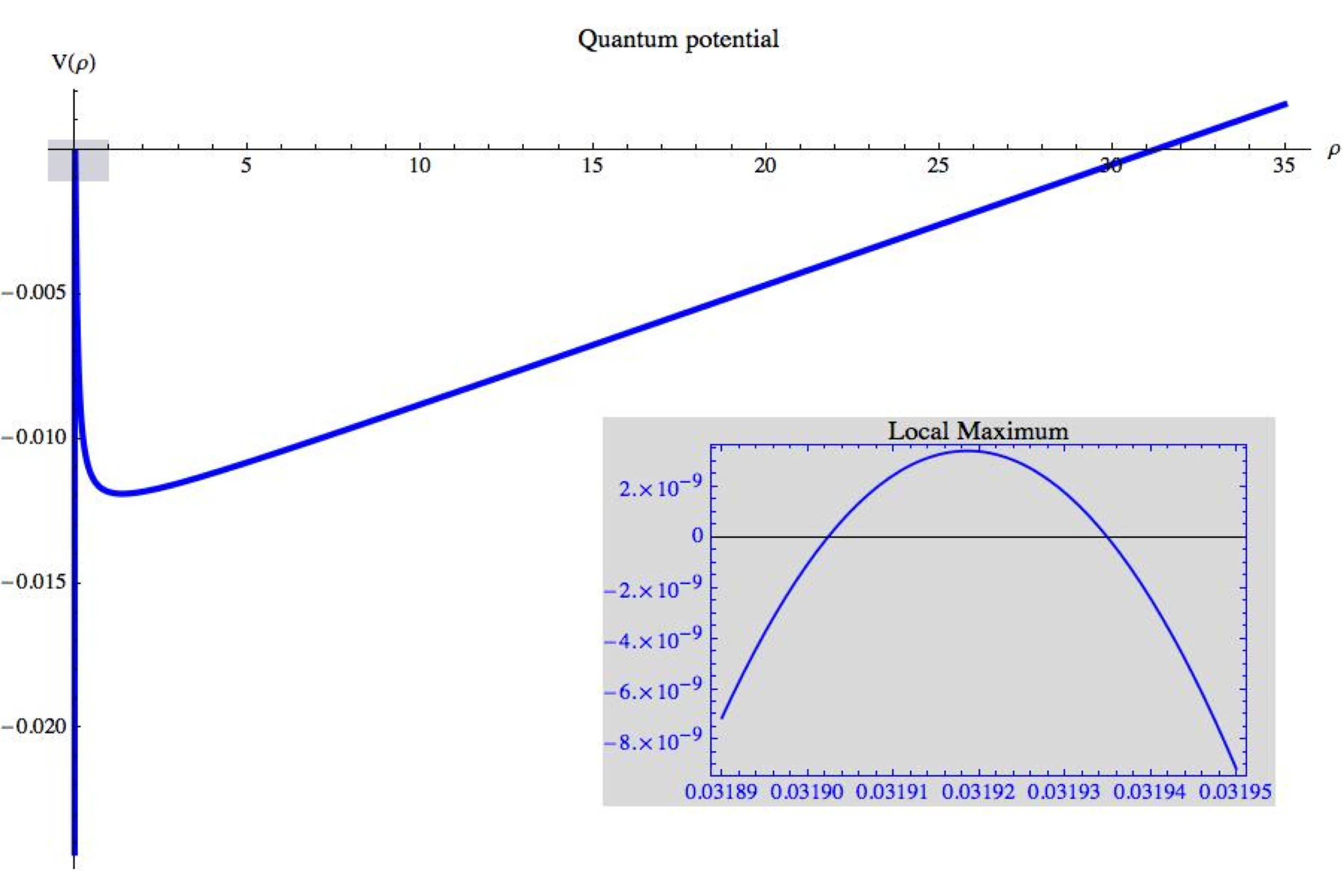
Figure 1: Effective quantum potential of a charged rigid bubble for large values of $\varrho$ and when $\varrho$ approaches to zero. For this graph we considered the energy value $\varepsilon=0.1144817$.

The issue of computing explicit solutions of the Eq. (22bj) results very complicated, instead we bring into a play a numerical technique based in a Fortran code in order to compute the energy spectrum. For this reason, it is convenient to choose the dimensionless quantities, $\varrho:=r/r_{0}$ and $\varepsilon=r_{0}\Omega$ (see for example [23]) where we have considered the results of the Subsection 4.1. Now, by a suitable alternative function $\phi(r):=\psi(r)/r$, the radial equation (22bj) becomes

$$\left(-\frac{d^{2}}{d\varrho^{2}}+V(\varrho)\right)\phi(\varrho)=0\,,$$ (22bl)

where

$$V(\varrho)=-\frac{\lambda^{2}}{4\varrho^{2}}+\frac{\varepsilon\lambda}{\varrho}+\frac{\varepsilon\lambda}{2}\,\varrho-\left(\varepsilon^{2}+\frac{\lambda^{2}}{4}\right)\,.$$ (22bm)

By employing the fourth-order Runge-Kutta method altogether with the necessary boundary conditions $\phi(0)=0$ and $\phi^{\prime}(0)=A$, the latter being an arbitrary value which is not relevant for the final result, we are able to obtain the solutions of the Eq. (22bl), [24]. Now, by using the shooting method, both the eigenfunctions and eigenvalues of the Schrödinger-like equation (22bl) can be computed. Some of the excited states eigenvalues of the charged bubble are shown in Table 1. Similarly, in Figure 2 we plot the first normalized eigenfunctions $\phi_{n}(\varrho)$. At this point, we are able to compare our results with those developed by Önder and Tucker in [4]. We found that for $n=1$, $\Omega_{1}=15.68\,\,m_{e}$ and for $n=133$, $\Omega_{133}=206.768\,\,m_{e}$ (the muon mass), unlike the values obtained by OT where, for instance, they found for the ground state $n=1$, $\Omega_{1}\simeq 13\,\,m_{e}$ and for $n=190$, $\Omega_{190}\simeq 200\,\,m_{e}$. This fact is a merely consequence of the several aspects of the quantum approach developed by OT where a semiclassical quantization, in a specific gauge, was adopted. Hence, the old idea pursued by Dirac regarding that the first excited state could be considered as a muon is not realized for this rigid bubble model.

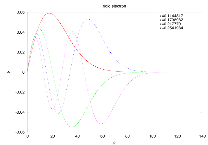
Figure 2: The first normalized eigenfunctions of a charged rigid membrane.

Table 1: Eigenvalues of the Schrödinger-like equation (22bl) and the excited energies of the charged bubble

• $n$	$\varepsilon_{n}$	$\Omega_{n}/m_{e}$
  1	0.1144817	15.6839929
  2	0.1738982	23.8240616
  3	0.2177701	29.8345146
  4	0.2541984	34.8251903
  5	0.2860303	39.1861634
  6	0.3146605	43.1085008
  7	0.3408957	46.7027122
  8	0.3652517	50.0394897
  9	0.3880928	53.1686423
  10	0.4096428	56.1210636

8 Concluding remarks

In this paper we reviewed the classical and quantum aspects of a rigid charged conducting membrane. We considered our model as a dynamical bubble in the presence of an electromagnetic field with the non-electromagnetic forces described by a term depending linearly on the extrinsic curvature of the worldvolume. As discussed before, though such correction term involves second-order derivatives, the ensuing equations of motion are of second-order in the field variables, as expected. We would like to remark that a generic minimal coupling term between the charge and the field $A_{\mu}$ has been considered in this work [11], and it is equivalent to the Dirac original proposal that introduces a coupling by means of a boundary condition which is consistent only in a particular gauge [1].

Our analysis took into consideration the routinely neglected boundary term which involves second-order derivatives of the configuration variables. Thus, we evoked the Ostrogradski-Hamiltonian formalism in order to investigate the constrained structure of the model. Indeed, a canonical transformation allowed us to acquire control over our set of constraints.. As expected, we are ushered to a Hamiltonian constraint which do not depend on the momenta associated to the higher-order variables, hence the structures coming from the boundary term do not play a relevant part on the dynamics of the system, but nonetheless they play the important role of being a bridge to obtain quadratic expressions in the physical momenta, useful for a passage to the quantum theory.

At the quantum level, we considered the canonical formalism of Dirac in order to overcome certain issues found in previous attempts by several other authors. In particular, we obtained a Schrödinger-like equation where the explicit effective quantum potential is identified, and the global behavior of the potential is discussed. As a byproduct, we have made a reappraisal of the excited states eigenvalues of this type of charged membrane which demonstrates the significant value of prediction of the scheme followed here.

More comments are in order. The Dirac model presents signals of instability [25]. Perhaps, this shortcoming could be overcome if we take into account a linear extrinsic curvature correction term in the model. Other proposals to eliminate the stability problem of the original Dirac model have been approached by considering a spinning bubble in the way studied in [26] or by the introduction of worldvolume fields pondering the spin of the electron [27]. Certainly, if a more complete model which includes the tension of the membrane is considered, we will not necessarily bring an improvement on the dynamical behavior since it will engender some singularities or discontinuities in the potential which can not be ruled out from the outset. This caveat must be scrutinized cautiously in the dynamical analysis and provides a good motivation for subsequent studies.

Finally, the model described here, results interesting in its own right since it has all the hallmarks of cosmological brane models. Among the brane cosmology concerns, we can mainly point two of them: their gravity and their dynamics. In this context, making use of the scheme here developed, it will be interesting to study the cosmology associated to the Dvali-Gabadadze-Porrati model, now taking into account a term depending linearly on the extrinsic curvature with the purpose to remove the pathologies and instabilities of such model [28]. An enormous advantage will be that the resultant effective model will retain a linear dependence on the acceleration of the field variables which open the possibility to apply the same quantum strategy followed here.

References

References

- [1] P. A. M. Dirac, Proc. R. Soc. A268 57 (1962).
- [2] A. Less, Philos. Mag.28 385 (1939).
- [3] M. Önder and R. W. Tucker, Phys. Lett. B202 501 (1988).
- [4] M. Önder and R. W. Tucker, J. Phys. A: Math. Gen. 21 3423 (1988).
- [5] R. Gregory, Phys. Rev. D43 520 (1991).
- [6] B. Carter and R. Gregory, Phys. Rev. D51 5839 (1995).
- [7] E. I. Guendelman and J. Portnoy, Class. Quantum Grav. 16 3315 (1999); arXiv:gr-qc/9901066v1.
- [8] A. Davidson and S. Rubin, Class. Quantum Grav.26 235006 (2009); arXiv:0907.1189v2 [gr-qc].
- [9] B-Y Chen, J. London Math. Soc. 6 321 (1973).
- [10] C. Barrabes, B. Boisseau and M. Sakellariadou, Phys. Rev. D49 2734 (1994).
- [11] O. A. Barut and M. Pavšič, Phys. Lett. B306 49 (1993).
- [12] A. Davidson and E. Guendelman, Phys. Lett. B251 250 (1990).
- [13] R. Capovilla and J. Guven, Phys. Rev. D51 6736 (1995); arXiv:gr-qc/9411060v2.
- [14] R. Capovilla, J. Guven and E. Rojas Class. Quantum Grav.21 5563 (2004); arXiv:hep-th/0404178.
- [15] R. Cordero, A. Molgado and E. Rojas, Phys. Rev. D79 024024 (2009); arXiv:0901.1938v1 [gr-qc].
- [16] T. Regge and C. Teitelboim, in Proceedings of the Marcel Grossman Meeting, Trieste, Italy, (1975), ed. R. Ruffini (North-Holland, Amsterdam) 77 (1977).
- [17] D. Karasik and A. Davidson, Phys. Rev. D67, 064012 (2003); arXiv:gr-qc/0207061v2.
- [18] A. Davidson, D. Karasik and Y. Lederer, Class. Quantum Grav. 16 1349 (1999).
- [19] P. A. M. Dirac, Lectures on Quantum Mechanics, Belfer Graduate School of Science, Yeshiva University, New York (1964).
- [20] M. Henneaux and C. Teitelboim, Quantization of Gauge Systems, Princeton University Press, (1992).
- [21] E. I. Guendelman and A. B. Kaganovich, Int. J. Mod. Phys. D2, 221 (1993).
- [22] R. Šteigl and F. Hinterleitner, Class. Quantum Grav. 23 3879 (2006); arXiv:gr-qc/0511149v1.
- [23] E. Stedile, Int. J. Theor. Phys. 43, 385 (2004).
- [24] N. J. Giordano and H. Nakanishi, Computational Physics, Prentice Hall, New Jersey, 2nd Ed., (2006).
- [25] P. Gnadig, P. Hasenfratz, Z. Kunnszt and J. Kuti, Annals Phys. 116, 380 (1978).
- [26] C. A. López, Phys. Rev. D33 2489 (1986).
- [27] A. Davidson and U. Paz, Phys. Lett. B300 234 (1993); arXiv:hep-th/9302081v1.
- [28] R. Gregory, N. Kaloper, R. C. Myers and A. Padilla, JHEP 10 069 (2007); arXiv:0707.2666v2 [hep-th].