Scale-dependent halo bias from scale-dependent growth

Abstract

We derive a general expression for the large-scale halo bias, in theories with a scale-dependent linear growth, using the excursion set formalism. Such theories include modified gravity models, and models in which the dark energy clustering is non-negligible. A scale dependence is imprinted in both the formation and evolved biases by the scale-dependent growth. Mergers are accounted for in our derivation, which thus extends earlier work which focused on passive evolution. There is a simple analytic form for the bias for those theories in which the nonlinear collapse of perturbations is approximately the same as in general relativity. As an illustration, we apply our results to a simple Yukawa modification of gravity, and use SDSS measurements of the clustering of luminous red galaxies to constrain the theory’s parameters.

I Introduction

The cosmological constant ($\Lambda$) + cold dark matter (CDM) + general relativity (GR) model has been very successful in accounting for current cosmological data. It is incumbent upon us to put this standard model to further tests. One of its characteristic predictions is a scale-independent sub-Hubble linear growth, which can be violated if dark energy clusters, or if gravity is modified Dvali et al. (2000); Nicolis et al. (2009); de Rham et al. (2010); Fierz (1956); Jordan (1959); Brans and Dicke (1961); Buchdahl (1970); Carroll et al. (2004). Both types of models introduce new scales into the growth of structure: the Jeans scale in the case of clustered dark energy, and the GR-to-non-GR transition scale in the case of modified gravity. The most direct way to test for this effect is to measure the matter power spectrum at different redshifts, and reconstruct the growth factor as a function of scale. Here, we focus on a corollary of a scale-dependent growth, a scale-dependent halo bias, which in principle allows us to discern scale dependence even with measurements of the large-scale structure at a single redshift.

The fact that a scale dependence in growth implies scale dependence in halo bias (on linear scales) was pointed out by Hui and Parfrey (2008) (henceforth HP), generalizing earlier work by Fry (1996); Tegmark and Peebles (1998):

$$b_{1}(k_{0},z_{\rm obs};z_{\rm form})=1+[b_{1}(z_{\rm form})-1]{D(k_{0},z_{\rm form})\over D(k_{0},z_{\rm obs})}$$ (1)

where $b_{1}(k_{0},z_{\rm obs};z_{\rm form})$ signifies the linear bias on scale $k_{0}$ observed at redshift $z_{\rm obs}$, for haloes that form at redshift $z_{\rm form}$. The symbol $D$ denotes the linear growth factor at the relevant scale and redshift. This expression, which assumes passive evolution, i.e. halo number conservation after formation, tells us that the observed bias would inherit a scale dependence from the growth, even if the formation bias is scale-independent. In this paper, we wish to relax these two assumptions: scale-independent formation bias, and no mergers.

The paper is organized as follows. The extended Press-Schechter, or excursion set, formalism Press and Schechter (1974); Bardeen et al. (1986); Bond et al. (1991); Lacey and Cole (1993); Sheth (1998) is described and generalized to allow for a scale-dependent growth in Sec. II. This is used to compute the halo mass function and the halo bias. In Sec. III, we describe an illustrative example, a modified gravity model of the Yukawa type, and present a calculation of the linear growth factor and the excursion barrier (collapse threshold). We present the halo bias for this example, and compare it with observations. We conclude in Sec. IV. In this paper, for the purpose of illustration, we have chosen to focus on one particular model of modified gravity. Our results in §II for the scale-dependent halo bias are, on the other hand, fairly general. A recipe for using these results in more general settings is summarized in Sec. IV. Readers who are interested primarily in applications, and not on the derivation, can skip directly to Sec. IV. In Appendix A we discuss some details concerning the use of the excursion set method for theories with a scale-dependent growth factor. In Appendix B we give the derivation of the Yukawa model from a scalar-tensor theory, and we describe our spherical collapse model in Appendix C.

Before we proceed, let us briefly discuss the connection with some of the literature on the subject. The halo mass function for a Yukawa theory like the one we study was computed by Martino et al. (2009). Our paper follows their formalism, and it is in a sense a straightforward extension to compute the conditional mass function and halo bias. Halo bias in $f(R)$ gravity and the DGP models has been measured from numerical simulations in Schmidt et al. (2009); Khoury and Wyman (2009); Schmidt (2009); Chan and Scoccimarro (2009); Schmidt et al. (2010) . They find fair agreement between simulations and the bias derived from a modified Sheth and Tormen Sheth and Tormen (1999) mass function whose parameters reflect the altered spherical collapse.

There is a large literature on testing GR using the growth of large-scale structure, e.g. Lue et al. (2004). Most studies allow for a scale-dependent growth factor, but ignore its effect on the galaxy bias. Our expression for the bias should be useful for incorporating the latter effect into such studies.

There is also a substantial literature on a large-scale scale-dependent bias from primordial non-Gaussianity, e.g. Dalal et al. (2008). This other source of scale dependence should be distinguishable from that from growth; we will discuss this in Sec. IV.

II Excursion set theory of haloes with a scale-dependent growth factor

We describe in detail here the excursion set formalism. Much of the discussion replicates the standard treatment, but with special care taken to allow for a scale-dependent growth factor.

II.1 Random walks

The premise of the excursion set theory is that a halo will form from a region of a certain size when the overdensity of matter $\delta$, smoothed over that region, is greater than a critical value $\delta_{\rm crit}$ Press and Schechter (1974). In FIG. 1, the mass overdensity, at a point, smoothed on a comoving scale $R$, is plotted against the variance $S$ on that scale around that point, where

$$S(R)=\int_{0}^{\infty}\frac{\mathrm{d}^{3}k}{(2\pi)^{3}}P(k)|\widetilde{W}(kR)|^{2}\,,$$ (2)

$P(k)$ is the matter power spectrum, and $\widetilde{W}(kR)$ the Fourier-space window function. As the smoothing scale is decreased, the smoothed density field undergoes a random walk. The halo mass $M$ is given by $M=(4\pi/3)\bar{\rho}(z=0)R^{3}$, where $\bar{\rho}$ is the mean matter density today. Hence, $M$, $S$ and $R$ can all be thought of as equivalent variables.

Figure 1: Random walks: notation for the excursion set model. A point is contained in a halo corresponding to the first upcrossing of the barrier, here $\delta_{\rm crit}$, by the random walk.

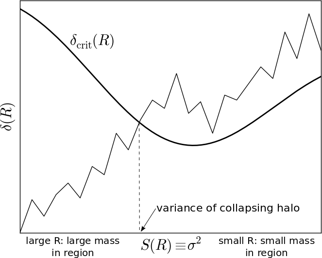
Following common practice, we smooth the density field with a real-space top-hat filter (even though, strictly speaking, a true random walk requires a top-hat filter in Fourier space Bond et al. (1991)). In an important sense all of our analysis is ‘native’ to real space; for all quantities not explicitly marked as being in Fourier space by a $\widetilde{\;\,}$, we define the wavenumber associated with a scale $R$ as simply $k\equiv 1/R$. The Fourier transform of a real-space top hat is

$$\widetilde{W}(kR)=\frac{3}{x^{3}}\left\{\sin(x)-x\cos(x)\right\}\,,\;x\equiv kR\,.$$

Following Martino et al. (2009), this random walk exercise is carried out at some initial redshift $z_{i}$, chosen to be early enough that the linear growth is scale-independent (i.e. neither dark energy nor modified gravity is important by this redshift). Throughout this paper we set $z_{i}=100$, although its precise value is not important as long as it is sufficiently early. We add the subscript $i$ to the critical threshold for halo formation $\delta_{\rm crit,i}$ to remind ourselves that it is the comparison between the smoothed $\delta_{m}$ at $z_{i}$ against this threshold that defines haloes. The value for $\delta_{\rm crit,i}$ in general depends on both the halo mass of interest (i.e. the barrier is not necessarily flat, unlike in the standard model), and the actual physical redshift of halo formation $z_{\rm form}$.

II.2 Unconditional first-crossing distribution & the mass function

The central quantity in the excursion set theory is the first-crossing distribution, $f$. Define $f(S_{1},\delta_{1}|0,0)\,\mathrm{d}S_{1}$ as the probability that a random walk starting at the origin will first cross the barrier, of height $\delta_{1}\equiv\delta_{\text{crit,i}}$, at $S=S_{1}\pm\mathrm{d}S_{1}/2$. This is equivalent to saying that $f(S_{1},\delta_{1}|0,0)|\mathrm{d}S_{1}/\mathrm{d}M_{1}|\,\mathrm{d}M_{1}$ is the probability that our point (around which this smoothing or random walk exercise is performed) belongs to a halo of mass $M_{1}\pm\mathrm{d}M_{1}/2$. We can think of $(S_{1},\delta_{1})$ as the target point we are aiming for on our random walk.

To find $f$, it is sometimes convenient to consider first the cumulative crossing distribution, $F$, which is the probability that the walk first crosses the barrier at $S<S_{1}$:

$$F(S_{1},\delta_{1}|0,0)=\int_{0}^{S_{1}}f(S,\delta|0,0)\,\mathrm{d}S\,,$$

where $\delta$ is the critical threshold $\delta_{\text{crit,i}}$, generally a function of $S$; in the case where it is $S$-independent, i.e. flat barrier, $F$ (and therefore $f=\partial F/\partial S_{1}$) can be found using a clever trick due to Chandrasekhar Chandrasekhar (1943), or by modelling the random walk as a diffusive process (see Bond et al. (1991); Lacey and Cole (1993)). For a more general barrier, an alternative method for finding $f$ will be discussed in §II.6. We assume that the probability distribution of the density field as a function of the smoothing scale $R$ is Gaussian:

$$P_{G}(\delta,S(R))d\delta=\frac{1}{\sqrt{2\pi S(R)}}\exp{[-\delta^{2}/2S(R)]}\,\mathrm{d}\delta\,.$$

Using the above, we see that the mass function of haloes (the physical number density of haloes as a function of mass, smoothed over the whole universe) which are identified at $z_{\text{form}}$ and observed at $z_{\text{obs}}$ is given by

$$n(M_{1})\mathrm{d}M_{1}=\frac{\bar{\rho}(z_{\text{obs}})}{M_{1}}f(S_{1},\delta_{1}|0,0)\left|\frac{\mathrm{d}S_{1}}{\mathrm{d}M_{1}}\right|\mathrm{d}M_{1}\,,$$ (3)

where $\bar{\rho}(z_{\text{obs}})$ is the mean matter density at $z_{\text{obs}}$. The mass function has an implicit dependence on $z_{\text{form}}$ through the dependence of the threshold/barrier $\delta_{1}$ on the formation redshift.

II.3 Conditional first-crossing distribution & halo bias

II.3.1 Lagrangian space

We can now move the starting point of our random walk away from the origin, to some other point on the $S$–$\delta$ plane. Call this point $(S_{0},\delta_{0})$. This is equivalent to calculating all our quantities within a region of the size on which the mass variance is $S_{0}$, and which has a mass overdensity $\delta_{0}$. The differential probability that a random walk starting from this point will first cross the barrier $\delta_{1}$ is $f(S_{1},\delta_{1}|S_{0},\delta_{0})$. In the flat-barrier case this only depends on $S_{1}-S_{0}$ and $\delta_{1}-\delta_{0}$.

Using this conditional first-crossing distribution we can construct an expression for the overdensity of haloes within a region of $(S_{0},\delta_{0})$ Mo and White (1996); Sheth and Lemson (1999). Just as we derived the unconditional mass function above, we can derive a conditional mass function. We can see from our definitions that the mean number $\mathcal{N}$ of $M_{1}$ haloes in a region of total mass $M_{0}$ is

$$\mathcal{N}(M_{1},\delta_{1}|M_{0},\delta_{0})=\frac{M_{0}}{M_{1}}f(S_{1},\delta_{1}|S_{0},\delta_{0})\left|\frac{\mathrm{d}S_{1}}{\mathrm{d}M_{1}}\right|\,,$$ (4)

and so their number density is $\mathcal{N}/V_{0}$ if the region has volume $V_{0}(M_{0})$.

We define the overdensity of haloes ‘1’ in a region ‘0’ as the fractional overabundance of these haloes in this region compared to their number density smoothed over the whole universe, giving

$$\delta_{h}^{L}(1|0)=\frac{\mathcal{N}(M_{1},\delta_{1}|M_{0},\delta_{0})}{n(M_{1},\delta_{1})V_{0}}-1\,.$$ (5)

This is the halo overdensity in Lagrangian co-ordinates, in which $M_{0}\approx\bar{\rho}(z_{i})V_{0}$, defining $V_{0}$. Indeed, all quantities in this Lagrangian space discussion, including $\delta_{0},V_{0},\delta_{1}$ and so on, are defined at the initial redshift $z_{i}$.

II.3.2 Eulerian space

In Eulerian co-ordinates we need to replace $V_{0}$ with the evolved Eulerian volume. In the above, the Lagrangian space quantities $V_{0}$ and $\delta_{0}$ are calculated at $z_{i}$. We now have three redshifts: the initial redshift $z_{i}$ (which we always set to 100), the identification redshift of the haloes $z_{\text{form}}$ (in a sense, their formation redshift), and the redshift at which the haloes are observed $z_{\text{obs}}$.

Label as $\delta$ the physical matter overdensity of the region of interest, at the observation redshift $z_{\text{obs}}$. It will be related to the Lagrangian space $\delta_{0}$ by

$$\delta=\frac{D(S_{0},z_{\text{obs}})}{D(S_{0},z_{i})}\,\delta_{0}\,,$$ (6)

because $\delta_{0}$ is defined at $z_{i}$. The use of the linear growth factor $D$ is justified for a small $S_{0}$, or correspondingly a large region. By the time of observation, the volume of the observed patch will have contracted from its Lagrangian-space value, because conservation of mass requires that the volume decreases as $\delta$ increases. Label as $V$ the volume of our region at $z_{i}$, taking into account the contraction it will experience by the time it reaches $z_{\text{obs}}$. Since $\delta(z_{i})\approx 0$, we find

$$M_{0}\approx\bar{\rho}(z_{i})V_{0}\equiv\bar{\rho}(z_{i})(1+\delta)V\quad\longrightarrow\quad V=\frac{V_{0}}{1+\delta}\,.$$

Substituting $V_{0}\rightarrow V$ into Eq. (5), and using Eqs. (3) and (4), gives the Eulerian halo overdensity $\delta_{h}^{E}$:

$$\delta_{h}^{E}=(1+\delta)\frac{f(S_{1},\delta_{1}|S_{0},\delta_{0}(\delta))}{f(S_{1},\delta_{1}|0,0)}-1\,.$$ (7)

It is clear that $\delta_{h}$ (dropping the ‘E’ from now on) will in general not be the same as the matter overdensity in the same region, $\delta$. A positive $\delta$ will usually help haloes reach the collapse threshold and increase their overdensity, with the opposite effect for negative $\delta$. There are also halo exclusion effects; for example, the halo density will be suppressed unless their mass is much smaller than the mass available in the region. From the random walk perspective, the ‘time’ available for barrier crossing is $S_{1}-S_{0}$, in which time the walk must travel a ‘distance’ $\delta_{1}-\delta_{0}$. You can suppress halo formation either by reducing the time available ($M_{\text{halo}}\equiv M_{1}$ approaching $M_{0}$) or by increasing the required distance (increasing the height of the barrier).

Since we know $\delta_{h}$ is a function of $\delta$, we can expand it as a Taylor series Fry and Gaztanaga (1993),

$$\delta_{h}=\sum_{k=0}^{\infty}\frac{1}{k!}b_{k}\delta^{k}\,.$$ (8)

The $b_{k}$ co-efficients are the bias parameters. The first, $b_{0}$, vanishes in the limit of $S_{0}\ll S_{1}$. Here, we are primarily concerned with $b_{1}$, the linear bias, in the $\delta\rightarrow 0$ limit (because we are interested in large regions, on which scales the mass overdensity is expected to be small). The linear bias in the limit $\delta\rightarrow 0$ is just $\partial\delta_{h}/\partial\delta$ evaluated at $\delta=0$, and so, using $\partial\delta_{0}/\partial\delta=D(S_{0},z_{i})/D(S_{0},z_{\text{obs}})$, we find

$$b_{1}(\delta\rightarrow 0) =\frac{1}{f(S_{1},\delta_{1}|0,0)}\Biggl{\{}f(S_{1},\delta_{1}|S_{0},0)$$

$$\quad+\frac{D(S_{0},z_{i})}{D(S_{0},z_{\text{obs}})}\left.\frac{\partial f(S_{1},\delta_{1}|S_{0},\delta_{0})}{\partial\delta_{0}}\right|_{\delta_{0}=0}\Biggr{\}}\,.$$ (9)

Recall that $S_{0}$, $R_{0}$, and $k_{0}$ are all equivalent variables; $S_{0}$ and $R_{0}$ are related by Eq. (2), and $k_{0}\equiv 1/R_{0}$. The $D(S_{0},z_{i})/D(S_{0},z_{\text{obs}})$ factor in this equation will make the large-scale bias scale-dependent in many modified gravity theories, or theories in which dark energy clusters in a non-negligible manner.

II.4 Flat barrier approximation

As we will see in §III, a flat barrier may be a good approximation for some theories. This is not surprising even for non-standard theories: haloes of a sufficiently small mass cross the barrier in a regime where essentially the standard story applies, i.e. the crossing occurs on small scales where gravity is Newtonian and dark energy typically is quite smooth. A useful analytic form for the halo bias can be written down in this case. The conditional first crossing distribution is Bond et al. (1991)

$$f(S_{1},\delta_{1}|S_{0},\delta_{0})=\frac{1}{\sqrt{2\pi}}\frac{\delta_{1}-\delta_{0}}{(S_{1}-S_{0})^{3/2}}\exp{\left[-\frac{(\delta_{1}-\delta_{0})^{2}}{2(S_{1}-S_{0})}\right]}\,,$$

and so, using Eq. (9), we find the Eulerian-space bias to be

$$b_{1} =\left(\frac{S_{1}}{S_{1}-S_{0}}\right)^{3/2}\left\{1+\frac{D(S_{0},z_{i})}{D(S_{0},z_{\text{obs}})}\left(\frac{\delta_{1}}{S_{1}-S_{0}}-\frac{1}{\delta_{1}}\right)\right\}$$

$$\quad\times\exp{\left[-\frac{\delta_{1}^{2}S_{0}}{2S_{1}(S_{1}-S_{0})}\right]}\,.$$ (10)

We are interested in scales on which $S_{0}\ll S_{1}$, i.e. the halo mass of interest is much smaller than the mass encompassed in the region over which we are calculating the clustering. Therefore,

$$b_{1}(S_{0},z_{\rm obs};z_{\rm form})=1+\frac{D(S_{0},z_{i})}{D(S_{0},z_{\text{obs}})}\left(\frac{{\delta_{1}}^{2}}{S_{1}}-1\right)\frac{1}{\delta_{1}}\,.$$ (11)

The bias $b_{1}$ depends on $z_{\rm form}$ because $\delta_{1}$ is the initial overdensity threshold for collapse at $z_{\rm form}$.

As a check, it can be seen this reduces to the Mo & White Mo and White (1996) result in the standard model, by recognizing that both $\delta_{1}$ and $S_{1}$ in our description are defined at the initial redshift $z_{i}$ — one can use part of the factor $D(S_{0},z_{i})/D(S_{0},z_{\rm obs})=[D(z_{i})/D(z_{\rm form})][D(z_{\rm form})/D(z_{\rm obs})]$ to rescale ${\delta_{1}}^{2}/S_{1}$ and $\delta_{1}$ down to $z_{\rm form}$ (recalling that $D$ is scale-independent in the standard model), and obtain $b_{1}=1+[D(z_{\rm form})/D(z_{\rm obs})](\nu^{2}-1)/\delta_{c}$, where $\delta_{c}$ is the linearly extrapolated overdensity of collapse at $z_{\rm form}$, and $\nu\equiv\delta_{c}/\sqrt{S_{1,\rm form}}$ with $S_{1,\rm form}$ being the the variance at $z_{\rm form}$ for our halo mass of interest $M_{1}$. The bias in its most familiar form obtains when one sets $z_{\rm form}=z_{\rm obs}$.

In non-standard models, Eq. (11) implies the linear bias $b_{1}$ is scale ($S_{0}$) dependent in general. The scale dependence comes entirely from the ratio of growth factor $D(S_{0},z_{i})/D(S_{0},z_{\rm obs})$. The result resembles Eq. (1) Hui and Parfrey (2008). To facilitate comparison, it is helpful to rewrite Eq. (11) as

$$b_{1}(S_{0},z_{\rm obs};z_{\rm form})=1+(b_{1}(S_{0},z_{\text{form}})-1)\frac{D(S_{0},z_{\text{form}})}{D(S_{0},z_{\text{obs}})},$$ (12)

where $b_{1}(S_{0},z_{\text{form}})$ is the formation bias, given by

$$b_{1}(S_{0},z_{\text{form}})=1+\frac{D(S_{0},z_{i})}{D(S_{0},z_{\text{form}})}\left(\frac{{\delta_{1}}^{2}}{S_{1}}-1\right)\frac{1}{\delta_{1}}$$ (13)

This is a trivial rewriting, but it makes clear that the formation bias $b_{1}(S_{0},z_{\text{form}})$ is in general scale-dependent, contrary to what was assumed in HP. It also helps differentiate between two different effects: one is the scale dependence at formation (from $D(S_{0},z_{i})/D(S_{0},z_{\text{form}})$ in Eq. [13]) , and the other is the scale dependence from passive evolution thereafter (from $D(S_{0},z_{\text{form}})/D(S_{0},z_{\text{obs}})$ in Eq. [12]).

Note that when $z_{\text{form}}\neq z_{\text{obs}}$, the haloes are identified at $z_{\text{form}}>z_{\text{obs}}$, and maintain their identities until $z_{\text{obs}}$. Mergers in the form of accretion onto these haloes are allowed between the two epochs, so long as the identification is unaltered, i.e. the haloes, once identified, are conserved. If this is not true — if the haloes continue to merge with each other all the way to $z_{\text{obs}}$ — then one should use $z_{\text{form}}=z_{\text{obs}}$. In this case, there is no distinction between the bias observed at $z_{\text{obs}}$ and the formation bias.

It is also instructive to further rewrite the formation bias using the following relations:

$$\delta_{1}=\delta_{1,{\rm form}}\frac{D(S_{1},z_{i})}{D(S_{1},z_{\text{form}})}\,,$$ (14a)

$$S_{1}=S_{1,{\rm form}}\frac{D^{2}(S_{1},z_{i})}{D^{2}(S_{1},z_{\text{form}})}\,,$$ (14b)

where we have introduced $\delta_{1,{\rm form}}$ and $S_{1,{\rm form}}$ for the linear overdensity threshold and the variance at $z_{\text{form}}$ (recall that our random walks are performed at the initial redshift $z_{i}$, hence $\delta_{1}$ and $S_{1}$ are defined then). The formation bias can thus be written as

$$b_{1}(S_{0},z_{\text{form}})=1+{D(S_{1},z_{\text{form}})\over D(S_{0},z_{\text{form}})}\left({{\delta^{2}_{1,{\rm form}}}\over S_{1,{\rm form}}}-1\right){1\over\delta_{1,{\rm form}}}\,,$$ (15)

where we have assumed that at a sufficiently early $z_{i}$, the growth factor is scale-independent, i.e. $D(S_{0},z_{i})=D(S_{1},z_{i})$. This is a useful expression because $\delta_{1,{\rm form}}$ is typically a constant, with fairly weak dependence on $z_{\text{form}}$ and cosmology (see footnote 3). This appears to be a good approximation even for the modified gravity model we will study below, where for sufficiently small haloes $\delta_{1,{\rm form}}$ approaches its $\Lambda$CDM value, which is $1.671$ for $z_{\text{form}}=0$.

II.5 The modified linear growth factor

So far, we have not been very explicit about where the scale-dependent growth factor actually comes from. On the sub-Hubble scales of interest, mass and momentum conservation imply the following equation for the linear matter overdensity $\delta$:

$$\frac{\mathrm{d}^{2}\delta}{\mathrm{d}a^{2}}+\left(\frac{3}{a}+\frac{1}{H}\frac{\mathrm{d}H}{\mathrm{d}a}\right)\frac{\mathrm{d}\delta}{\mathrm{d}a}=\frac{1}{a^{4}H^{2}}\nabla^{2}\phi\,,$$ (16)

where the Laplacian is in comoving coordinates. What modified gravity, or clustering in dark energy, does is to modify the relation between $\delta$ and the gravitational potential $\phi$, from the standard Poisson equation. The result can often be modelled as replacing $\nabla^{2}\phi$ by ${\cal O}\cdot\delta$, where ${\cal O}$ is some linear operator which can be scale-dependent, giving rise to a scale-dependent growth for $\delta$. Solving the resulting equation in Fourier space would give $\delta(k,z)=[\widetilde{D}(k,z)/\widetilde{D}(k,z_{i})]\delta(k,z_{i})$, where $k$ is the wavenumber of interest. We use the symbol $\widetilde{D}$ to distinguish this growth factor from the growth factor $D$ we use in the excursion set calculation. The difference arises from the fact that the excursion set calculation cares about the growth of the variance $S$, smoothed on scale $R$, or equivalently, $M$. We define $D$ in such a way to give the correct evolution of the variance $S$:

$$D^{2}(R,z)\equiv\frac{S(R,z)}{S(R,z_{i})}\,,$$ (17a)

$$\qquad=\int_{0}^{\infty}{\mathrm{d}^{3}k\over(2\pi)^{3}}P(k,z_{i})\left\{\widetilde{W}(kR)\frac{\widetilde{D}(k,z)}{\widetilde{D}(k,z_{i})}\right\}^{2}\biggr{/}$$

$$\qquad\qquad\qquad\int_{0}^{\infty}{\mathrm{d}^{3}k\over(2\pi)^{3}}P(k,z_{i})\widetilde{W}^{2}(kR)\,.$$ (17b)

In the excursion set computation, the overdensity $\delta$ is evolved using the same growth factor $D$. In practice, the integral over $k$ is expected to be dominated by $k\sim 1/R$, and therefore $D(R,z)$ is roughly $\tilde{D}(k=1/R,z)$, though we do not use this approximation.

II.6 Calculating the first-crossing distributions

As mentioned above, the flat barrier approximation turns out to be a fairly good one for the example we study. However, in general, the barrier or threshold for collapse is mass/scale-dependent. The corresponding first-crossing distribution can be found as follows.

First of all, it is possible to calculate the $f$ distribution analytically for barriers which are linear functions of $S$: if $\delta_{1}(S)=\omega-\beta S$,

$$f(S_{1},\delta_{1}|S_{0},\delta_{0})=\frac{\Delta\delta}{\Delta S\sqrt{2\pi\Delta S}}\exp{\left\{-\frac{\left(\Delta\delta-\beta\Delta S\right)^{2}}{2\Delta S}\right\}}\,,$$

where $\Delta\delta\equiv\delta_{1}(S_{0})-\delta_{0}$ and $\Delta S\equiv S_{1}-S_{0}$ Sheth (1998). For a more general barrier, there is no exact analytic solution, but reasonable approximations have been worked out by Sheth & Tormen, and Lam & Sheth Sheth and Tormen (2002); Lam and Sheth (2009). In this paper, we adopt the algorithm of Zhang & Hui Zhang and Hui (2006) which gives an exact, albeit numerical, solution for the unconditional $f$-function. It is straightforward to extend their method to the conditional case. It can be shown that the function is the solution of the integral equation

$$f(S_{1},\delta_{1}(S_{1})|S_{0},\delta_{0}) =g_{1}[S_{1},\delta_{1}(S_{1});S_{0},\delta_{0}]$$

$$\quad+\int_{S_{0}}^{S_{1}}\mathrm{d}S^{\prime}_{1}\,g_{2}[S_{1},\delta_{1}(S_{1});S^{\prime}_{1},\delta_{1}(S^{\prime}_{1})]$$

$$\qquad\times f(S^{\prime}_{1},\delta_{1}(S^{\prime}_{1})|S_{0},\delta_{0})\,,$$

where

$$g_{1}[S_{1},\delta_{1}(S_{1});S_{0},\delta_{0}] =\left\{\frac{\delta_{1}(S_{1})-\delta_{0}}{S_{1}-S_{0}}-2\frac{\mathrm{d}\delta_{1}}{\mathrm{d}S_{1}}\right\}$$

$$\quad\times P_{G}(\delta_{1}(S_{1})-\delta_{0},S_{1}-S_{0})\,,$$

$$g_{2}[S_{1},\delta_{1}(S_{1});S^{\prime}_{1},\delta_{1}(S^{\prime}_{1})] =\left\{2\frac{\mathrm{d}\delta_{1}}{\mathrm{d}S_{1}}-\frac{\delta_{1}(S_{1})-\delta_{1}(S^{\prime}_{1})}{S_{1}-S^{\prime}_{1}}\right\}$$

$$\quad\times P_{G}(\delta_{1}(S_{1})-\delta_{1}(S^{\prime}_{1}),S_{1}-S^{\prime}_{1})\,.$$

This is a Volterra equation of the second kind. By treating $f$ as a vector $f$, we can see that this equation is of the form $\mbox{\boldmath{$f$}}=\mbox{\boldmath{$g$}}+\mbox{\boldmath{$Mf$}}$ where $g$ is another vector and $M$ is a matrix, implying that $f$ can be found with a matrix inversion: $\mbox{\boldmath{$f$}}=(\mbox{\boldmath{$I$}}-\mbox{\boldmath{$M$}})^{-1}\mbox{\boldmath{$g$}}$. $M$ is a triangular matrix, allowing $\mbox{\boldmath{$I$}}-\mbox{\boldmath{$M$}}$ to be inverted efficiently by iteration Press et al. (1992).

III An illustration with a Yukawa model

By the Yukawa model, we mean using the following effective Poisson equation to compute the growth of perturbations and the formation of haloes (for instance, it goes into the right hand side of Eq. [16]):

$$-k^{2}\phi=4\pi\frac{G_{N}}{1+\alpha}\bar{\rho}a^{2}\delta\left[1+\alpha\frac{k^{2}}{k^{2}+a^{2}/\lambda^{2}}\right]\,,$$ (18)

which is written in Fourier space. Here, $G_{N}$ is the effective Newton’s constant at high $k$. The $k^{2}/(k^{2}+a^{2}/\lambda^{2})$ term corresponds to a Yukawa modification, where $1/\lambda$ can be thought of as a mass: it determines on what scale modifications to GR become important. The parameter $\alpha$ quantifies the size of the modification, i.e. the ratio of effective Newton’s constant on small scales to on large scales is $1/(1+\alpha)$. A positive $\alpha$ corresponds to weakening gravity on large scales (large compared to $\lambda$), while a negative $\alpha$ (but $>-1$) corresponds to the opposite.

This effective Poisson equation can be solved by

$$\phi(\mbox{\boldmath{$r$}})=-\frac{G_{N}}{1+\alpha}\int\mathrm{d}^{3}\mbox{\boldmath{$r$}}^{\prime}\,\frac{\bar{\rho}\delta(\mbox{\boldmath{$r$}}^{\prime})}{|\mbox{\boldmath{$r$}}-\mbox{\boldmath{$r$}}^{\prime}|}\left\{1+\alpha\exp{\left(-|\mbox{\boldmath{$r$}}-\mbox{\boldmath{$r$}}^{\prime}|/\lambda\right)}\right\}\,,$$ (19)

where $r$ is the physical proper coordinate, related to the comoving coordinate $x$ by $\mbox{\boldmath{$r$}}=a\mbox{\boldmath{$x$}}$.

The model encapsulated by Eq. (18) is phenomenological in nature. For a positive $\alpha$, it can be derived from a scalar-tensor theory with a potential for the scalar field, described in Appendix B.

One implication of Eq. (19) is that Birkoff’s theorem, or Gauss’s law, no longer holds: a test particle in a spherically-symmetric matter distribution feels a force from the matter both inside and outside the surface of constant radius defined by its position.

We investigate three methods, one exact and two approximate, for solving for the nonlinear evolution of spherically-symmetric perturbations, the details of which are deferred to Appendix C. This nonlinear problem has to be solved to determine the appropriate collapse threshold $\delta_{{\rm crit},i}$ used in the excursion set calculation. The violation of Birkoff’s theorem implies an initially top-hat perturbation does not remain so. However, we find that modelling the spherical perturbation as homogeneous (i.e. a top hat) at every time step is a good approximation for the parameters and halo masses of interest. Other infra-red modifications of gravity, such as DGP, appear to share the same feature —Schaefer & Koyama have argued Schaefer and Koyama (2008) that the effect of the violation of Birkoff’s theorem in DGP gravity should be small.

We find that a Yukawa-type modification of gravity, which is consistent with observations of galaxy clusters and hence has $\lambda>5\,h^{-1}\,\text{Mpc}$, will only affect the collapse dynamics for haloes with mass $M\gtrsim 10^{14}\,h^{-1}\,\text{M}_{\odot}$; for smaller haloes the evolution is basically GR-like. This is consistent with previous studies of spherical collapse of large haloes in Yukawa-modified gravity Martino et al. (2009).

In the rest of this section, we present results for the barrier $\delta_{{\rm crit},i}$ from the spherical collapse computation, and for the halo bias $b_{1}$ from the excursion set method. The background cosmology is taken to be that of $\Lambda$CDM (see Appendix B for discussions on consistency with modifying gravity for the perturbations). For the power spectrum, we use the analytic fit from Eisenstein and Hu (1998), with parameters fixed by the WMAP 5-year analysis: $\Omega_{\rm CDM}=0.206$, $\Omega_{\rm baryon}=0.043$, $\Omega_{\Lambda}=1-(\Omega_{\rm CDM}+\Omega_{\rm baryon})$, $n_{s}=0.961$, $h=0.724$ Komatsu et al. (2009). We normalize the power spectrum at a high redshift ($z_{i}=100$), i.e. the primordial normalization is the same for both the standard and non-standard models. The amplitude is chosen such that, if GR were to hold, $\sigma_{8}$ would equal $0.787$ today.

III.1 Barriers

(a) Examples for $\alpha=-0.5$, for different $\lambda$, as given in units of $\,h^{-1}\,\text{Mpc}$ beside each curve.

(b) Examples for $\lambda=10\,h^{-1}\,\text{Mpc}$, for different $\alpha$, given beside each curve. Note the log scale on the y-axis.

Figure 2: Barriers in Yukawa models parametrized by $\alpha$ and $\lambda$: the overdensity at $z_{i}=100$ required on each comoving scale $k_{1}$ or mass scale $M_{1}$, in order for that region to collapse by $z_{\text{form}}=0$.

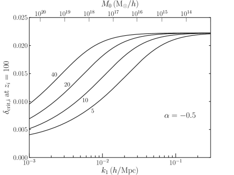
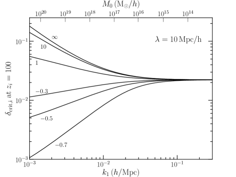
The barrier used in the random walk calculation is the initial overdensity required for a perturbation to collapse to zero radius by an identification redshift $z_{\text{form}}$. In general relativity the required initial overdensity is independent of scale, i.e. the barrier is flat. Curved barriers have been used to model the effect of ellipsoidal, rather than spherical, collapse; e.g. see Sheth et al. (2001).

For the Yukawa model, the barrier can be generated using the spherical collapse calculation outlined in Appendix C; in what follows we use the homogeneous sphere approximation throughout. For each scale $k_{1}$ ($\equiv 1/R_{1}$, or a mass of $M_{1}$), the initial overdensity is found which collapses at $z_{\text{form}}$. This defines $\delta_{\text{crit,i}}$, which is equated with $\delta_{1}$ in the excursion set theory, as a function of $k_{1}$ or $M_{1}$. FIG. 2 shows barriers for the Yukawa model with a range of parameter values for $\alpha$ and $\lambda$. At smaller $k_{1}$ in the weaker-gravity case ($\alpha>0$), the barrier is higher because these larger-scale perturbations enter the weakened-gravity regime earlier and experience more of a reduction in the gravitational force, and so need a larger initial overdensity to push them over the edge into collapse; the converse holds for the stronger-gravity ($\alpha<0$) model. At high $k_{1}$ the barrier approaches the GR result, which can be thought of as the value $1.671$, scaled back to $z_{i}=100$ using the $\Lambda$CDM growth factor ratio $D(z_{i})/D(z_{\text{form}})$. While not a focus of this paper, FIG. 2 suggests the mass function at the high mass end would be significantly affected by the curving of the barrier, especially its lowering at high mass for $\alpha<0$. The observed cluster count already constrains $\alpha$ to be not too negative Martino et al. (2009).

Figure 3: Ratio of simple (flat barrier, Eq. 10) to full (curved barrier, Eq. 9) bias expressions, for $\alpha=-0.5$, $\lambda=8\,h^{-1}\,\text{Mpc}$, $z_{\text{obs}}=z_{\text{form}}=0$.

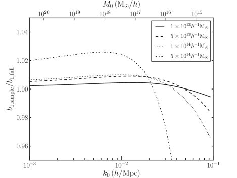
Anticipating the linear halo bias that we will calculate next, in FIG. 3 we plot the ratio of the flat barrier solution, Eq. (10), to the full curved barrier solution, Eq. (9) using the numerical procedure of Sec. II.6, for four halo masses. The amplitude of the flat barrier is taken to be the collapse threshold $\delta_{1}$ at high $k_{1}$, which in the case of our models is very close to the Newtonian value. The flat barrier approximation is very good for galaxy-mass haloes—for a halo of $10^{13}\,h^{-1}\,\text{M}_{\odot}$, the fractional discrepancy in the bias is of order $10^{-3}$ for the parameters considered. Decreasing $|\alpha|$, increasing $\lambda$, or increasing $z_{\text{form}}$ will flatten the barrier, further reducing this difference. Effects due to barrier curvature are more readily apparent for cluster-mass haloes, because the barriers in FIG. 2 are only curved at large masses.

III.2 Formation bias

There are two ways in which the halo formation bias (i.e. halo bias with $z_{\text{form}}=z_{\text{obs}}$) differs from the standard expression, due to for instance a modification to the gravitational law. One is from the scale-dependent linear growth, the other is from the curved barrier. The former is the dominant effect. As we have seen already from FIG. 3, the curvature of the barrier does not have a significant impact on the halo bias, on scales $k_{0}\mathrel{\hbox to0.0pt{\lower 4.0pt\hbox{\hskip 1.0pt$\sim$}\hss}\raise 1.0pt\hbox{$<$}}0.05$ h/Mpc. The impact on smaller scales is higher, but still minor for sufficiently light haloes.

Our most general expression for the halo bias is given by Eq. (9). The factor of $D(S_{0},z_{i})/D(S_{0},z_{\text{obs}})$ encapsulates the first effect. For instance, in the Yukawa model with $\alpha>0$ (weaker gravity on larger scales), this factor is larger on large scales, and the halo bias is correspondingly higher. Physically, what drives the higher halo bias on larger scales is this: recall that we are interested in how the halo overdensity $\delta_{h}$ relates to the matter overdensity $\delta$ at redshift $z_{\text{obs}}$; for a fixed $\delta$, the overdensity $\delta_{0}$ at the initial redshift $z_{i}$ (where the random walk is performed) is higher on larger scales if $\alpha>0$. This larger $\delta_{0}$ boosts halo formation, and results in a higher halo bias.

The curved barrier is in principle another way in which a scale dependence is imprinted on the halo bias. For this to occur, the barrier must absorb some trajectories before they reach ($S_{1}$,$\,\delta_{1}(S_{1})$) in a way which depends on the starting point $S_{0}$. We do not observe this in the models we consider, because on large scales the random walk has a negligible probability of crossing the barrier because the variance of each step, $S$, is so low. Therefore large-scale changes to the barrier have very little effect on the bias. (If $\alpha$ is strongly negative, say $\alpha\sim-0.7$, the barrier is so low on large scales that it absorbs the random walk paths before they reach ‘sensible’ halo scales, see FIG. 2(b). This produces a strongly scale-dependent bias and drastic under-production of low-mass haloes, which is clearly incompatible with observations.)

(a) $\alpha=1.0$, $\lambda=10\,h^{-1}\,\text{Mpc}$.

(b) $\alpha=-0.5$, $\lambda=10\,h^{-1}\,\text{Mpc}$.

Figure 4: Bias versus scale for $z_{\text{form}}=z_{\text{obs}}=0$. The halo masses in each case are, in units of $\,h^{-1}\,\text{M}_{\odot}$, $5\times 10^{14}$ (most biased), $10^{14}$, $5\times 10^{13}$, $10^{13}$, $5\times 10^{12}$, and $10^{12}$ (least biased). For the three largest masses, the curves are discontinued beyond the scale at which halo exclusion becomes important, i.e. where $M_{1}/M_{0}=0.01$. The panels illustrate the predictions for two Yukawa models.

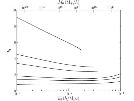
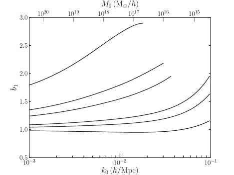
FIG. 4 shows the halo bias computed using the full excursion set theory, with a barrier determined by the exact spherical collapse calculation. The scale dependence of the bias comes almost entirely from the large-scale growth factor, and is well described by our flat-barrier expressions, Eqs.  (11), (13), or (15). As the halo mass increases (and so the variance $S_{1}$ decreases) the factor multiplying the scale-dependent growth factor ratio, $({\delta_{1}}^{2}/S_{1}-1)/\delta_{1}$, becomes larger, leading to more pronounced scale dependence in the formation bias. The different curves in FIG. 4 are produced by the same scale-dependent factor multiplying a mass-dependent amplitude.

Figure 5: Passive bias evolution of a $5\times 10^{12}\,h^{-1}\,\text{M}_{\odot}$ halo which forms at $z_{\text{form}}=1$ and is observed at $z_{\text{obs}}=1$ (top), 0.5, and 0 (bottom); in this case $\alpha=-0.5$, $\lambda=10\,h^{-1}\,\text{Mpc}$.

III.3 Passive bias evolution

In the previous section we observed the haloes at the time of their formation. Some galaxy populations form at an early redshift and then evolve passively, without further major merger events. In this scenario the total number of haloes is conserved after the formation epoch; the haloes increase their mass only by accreting much smaller haloes. The mass assigned to the haloes is their mass at formation, disregarding subsequent accretion.

Here $z_{\text{form}}\neq z_{\text{obs}}$; the formation redshift determines the barrier shape and height via $\delta_{1}=\delta_{\text{crit,i}}$ (this is the initial overdensity threshold which has to be evolved back from the formation redshift), while the observation redshift determines the relationship between $\delta_{0}$ and $\delta$, Eq. (6). This combination reproduces, in the excursion set formalism, the modified-gravity bias-evolution results previously derived from the perturbation equations by HP Hui and Parfrey (2008), in the sense that $b_{1}-1$ scales with $D(S_{0},z_{\text{form}})/D(S_{0},z_{\text{obs}})$, as in Eq. (12). However, it should be kept in mind that according to the excursion set theory, the formation bias is not scale-independent in general, but is instead given by Eq. (13).

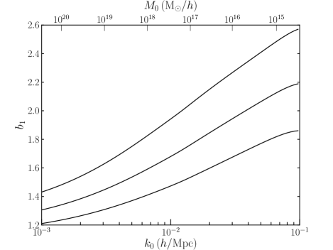
The combined effects of formation bias and passive bias evolution can be non-intuitive. For example, in FIG. 5 the stronger large-scale gravity ($\alpha<0$) causes the bias to be smaller on large scales, but passive evolution decreases the smaller scale bias faster. This is because on smaller scales the bias is greater, and thus is more quickly diluted by passive evolution.

III.4 Comparison with observations — an example

For comparison with observations, it is sometimes convenient to consider an apparent bias $b_{\text{app}}$, defined as

$$b_{\text{app}}(k_{0})\equiv\frac{D(k_{0},z_{\text{obs}})}{D(k_{0},z_{i})}\frac{D_{\Lambda{\rm CDM}}(z_{i})}{D_{\Lambda{\rm CDM}}(z_{\text{obs}})}b_{1}(k_{0})\,,$$ (20)

where $D_{\Lambda{\rm CDM}}$ is the growth factor according to the standard $\Lambda$CDM model, and $D$ is that according to our non-standard model. This is constructed such that the power spectrum of haloes in the non-standard model $P_{\rm haloes}$ is related to the matter power spectrum in $\Lambda{\rm CDM}$ $P_{\Lambda{\rm CDM}}$ by

$$P_{\text{haloes}}=b_{\text{app}}^{2}(k)P_{\Lambda\text{CDM}}\,.$$ (21)

This is a necessary step when we don’t know the matter power spectrum directly, and so must compare the observed galaxy distribution to what would be expected from an underlying standard-gravity matter distribution. If the matter power spectrum were known, from weak lensing for example, we could compare the measured bias to the true bias $b_{1}$ directly.

(a) $\alpha=1.0$, $\lambda=10\,h^{-1}\,\text{Mpc}$. Compare with FIG. 4(a).

(b) $\alpha=-0.5$, $\lambda=10\,h^{-1}\,\text{Mpc}$. Compare with FIG. 4(b).

(c) Passive apparent bias evolution of a $5\times 10^{12}\,h^{-1}\,\text{M}_{\odot}$ halo; $z_{\text{form}}=1.0$, $z_{\text{obs}}=1.0$ (solid), 0.5 (dashed), 0 (dashed-dotted). Compare with FIG. 5.

Figure 6: Birth and evolved apparent (rather than physical) biases for the same parameters and halo masses as FIG. 4 and FIG. 5.

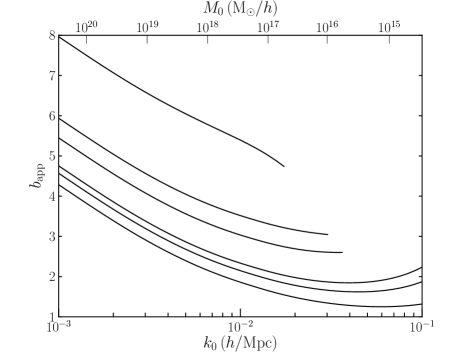
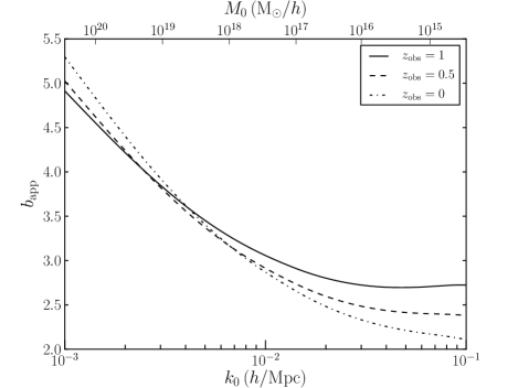
The apparent bias is plotted against scale in FIG. 6. On large scales the apparent bias has a constant slope, which is the same for all halo masses. This is because the form of the true bias, $b_{1}\approx 1+f_{1}(k_{0})f_{2}(M_{1})$ (Eq. 11), when multiplied by the scale-dependent factor $D(k_{0},z_{\text{obs}})/D(k_{0},z_{i})$, becomes $b_{\text{app}}\approx g_{1}(k_{0})+g_{2}(M_{1})$.

In FIG. 6(c), the large-scale apparent bias actually increases with passive evolution—this is due to the overall multiplicative factor in front of $b_{1}$ in the previous equation, which is greater than one on large scales when $\alpha<0$. The opposite occurs for positive $\alpha$: the large-scale apparent bias drops faster than the physical bias.

Figure 7: Galaxy biases derived from the SDSS LRGs, with Yukawa and Newtonian best fit curves. The best fit parameters are $\alpha=0.065$, $\lambda=6.5\,h^{-1}\,\text{Mpc}$

(a) $\alpha>0$

(b) $\alpha<0$

Figure 8: Contours of constant $\Delta\chi^{2}$ in the $\alpha$–$\lambda$ plane. The regions containing $\alpha=0$ are ‘included’ by the contours.

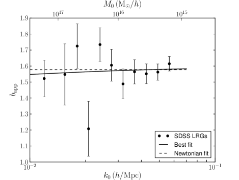
The high intrinsic luminosity of luminous red galaxies (LRGs) makes them useful tracers of the large-scale cosmic density field. We calculate the galaxy bias of the LRGs as a function of scale, using the LRG power spectrum derived from the SDSS galaxy redshift survey Tegmark et al. (2006), and the standard matter power spectrum, whose parameters are set to the WMAP 5-year maximum-likelihood values Komatsu et al. (2009). The LRGs are mostly believed to occur as the largest galaxy in individual haloes, and so the galaxy bias is approximately the host halo bias.

A description of the halo clustering with only the first bias parameter and the matter power spectrum is consistent only on linear scales, which we estimate here as those scales where the scale dependence introduced into the bias by a non-zero $S_{0}(k_{0})$ in Eq. 10 is small. This restricts our analysis of the LRG power spectrum to the eleven data points available for $k_{0}\lesssim 0.06\,h\,\text{Mpc}^{-1}$.

The LRGs may be a passively evolving population Masjedi et al. (2008) (however, see Wake et al. (2008) for an opposing view). Despite this, we use the formation bias at the median redshift of the sample, $z_{\text{form}}=z_{\text{obs}}=0.35$, in order to include any mass the haloes may have accreted since they formed. Ideally, one would bin the galaxies by redshift and account for the changing predicted bias shape for each modified gravity model, thus providing two tests: the shape of the bias curve at each redshift, and the evolution of the bias (in both shape and magnitude) with time. This may be feasible with future data sets.

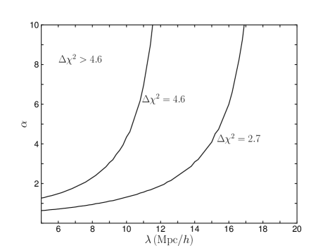
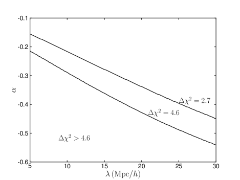
A complete analysis would include marginalization over the matter spectral index and $\sigma_{8}$. To derive some preliminary constraints, we fix all the properties of the matter power spectrum and ($\Lambda$CDM) expansion history, and marginalize over halo mass in a $\chi^{2}$ minimization procedure for each combination of $\alpha$ and $\lambda$. Fitting the apparent formation bias at the median redshift of the LRG sample gives best-fit parameters $\alpha=0.065$, $\lambda=6.5\,h^{-1}\,\text{Mpc}$, $M_{1}=1.2\times 10^{13}\,h^{-1}\,\text{M}_{\odot}$, with $\chi^{2}=10.08$. This is statistically indistinguishable from the Newtonian fit, with $\chi^{2}=10.21$. In fact, one could argue that the data does not favor the Yukawa model since it requires more parameters without improving $\chi^{2}$ much. However, the error bars are at the moment rather large. The observed biases and model fits are shown in FIG. 7.

FIG. 8 shows contours of constant $\Delta\chi^{2}$ in the $\alpha$–$\lambda$ plane. Marginalization over $\alpha$ or $\lambda$ is poorly constraining, since in both cases the Newtonian limit ($\alpha\rightarrow 0$ or $\lambda\rightarrow\infty$) is allowed, and so the marginalized $\Delta\chi^{2}$ cannot be larger than 0.13. This method places better limits on stronger-than-Newtonian-gravity models. These constraints should be considerably improved by future galaxy clustering measurements, especially those on scales $k_{0}<0.1\,h\,\text{Mpc}^{-1}$.

IV Conclusions

We have worked out the large-scale halo bias $b_{1}$ in a theory that has a scale-dependent linear growth, such as modified gravity or clustered dark energy. We give several expressions in §II.3 & II.4. The most general expression is Eq. (9). It relates $b_{1}$ to the first crossing distribution $f$, which can be computed using the method described in §II.6, for a general curved barrier. Note that all quantities describing the random walk: $\delta_{1},S_{1},\delta_{0},S_{0}$ are defined at the initial redshift $z_{i}$, as opposed to the formation redshift $z_{\rm form}$.

A much simpler expression, Eq. (15), obtains in cases where the barrier can be approximated as flat. As can be seen in the example depicted in FIG. 2, the barrier is generally not flat once a scale-dependent growth factor is allowed. However, it is often true that the barrier deviates from flatness only for the largest masses, and a flat barrier approximation (set at the small mass level) actually works quite well in predicting the halo bias for more modest halo masses (FIG. 3). The expression in Eq. (15) is particularly easy to use because the threshold for collapse $\delta_{1,{\rm form}}$ and the variance $S_{1,{\rm form}}$ are defined at the formation redshift as usual.

Our main result is the imprinting of a scale dependence on the formation bias, by the modified linear growth factor. This can be understood to occur because regions of the same overdensity but different sizes today would not all have had the same overdensity at an earlier redshift, and hence would have varying halo densities (see Sec. III.2). The scale dependence of the growth factor manifests itself at a single redshift, making it possible to look for it with a local-universe snapshot. Using this effect and an appropriate galaxy sample, one can place constraints on gravity theories, as we demonstrate with a simple Yukawa theory.

We have focused on the case in which the formation bias is deterministic. However, this bias may be stochastic, in which case this stochasticity will also be scale-dependent Hui and Parfrey (2008). Although we will not perform a detailed analysis of stochastic bias here, we note that, even if the formation bias is deterministic in, say, $k$-space, the scale dependence means that it will be stochastic in real space (and vice-versa) Desjacques and Sheth (2010). Thus, the stochasticity of the bias is another potential signature of modified gravity theories.

Looking forward, it would be interesting to work out how a scale-dependent large-scale bias can be incorporated into optimal weighting schemes for recovering the mass distribution from a galaxy or halo catalog Hamaus et al. (2010); Cai et al. (2010).

Appendix A Density field extrapolation

In an excursion set calculation, there are in principle four different redshifts that might be relevant: the initial redshift $z_{i}$ (taken to be $100$ in this paper), the formation redshift $z_{\rm form}$, the observation redshift $z_{\rm obs}$, and the redshift at which all the random walk variables (the variances $S_{0}$, $S_{1}$, etc) are defined: let us call it $z_{\text{fields}}$, or the random walk redshift.

In the standard theory, i.e. GR, the choice of $z_{\text{fields}}$ is immaterial. The simplest way to see this is to examine the flat barrier (but otherwise general) expression for bias in Eqs. (12) and (13). In this expression, the random walk variables $\delta_{1}$ and $S_{1}$ are defined at the initial redshift $z_{i}$. In other words, the choice $z_{\text{fields}}=z_{i}$ has been made. It is simple to see that if the growth factor $D$ were scale-independent, choosing a different random walk redshift, i.e. $z_{i}\rightarrow z_{\text{fields}}\neq z_{i}$ would have made no difference to the predicted bias. This is because in the expression for the formation bias (Eq. [13]), $\delta_{1}^{2}/S_{1}$ is independent of the random walk redshift by definition, and $\delta_{1}D(S_{0},z_{\rm form})/D(S_{0},z_{\text{fields}})$ (with $\delta_{1}$ defined at $z_{\text{fields}}$) is also independent of $z_{\text{fields}}$. The key is that the growth factor relevant for $\delta_{1}$, which is on scale $S_{1}$, is the same as the growth factor on scale $S_{0}$. This is true in GR, but not true for non-standard theories where the growth factor is generally scale-dependent. Indeed, in the standard theory, it is common practice to choose $z_{\text{fields}}=z_{\text{form}}$, such that for instance in an Einstein-de Sitter universe, $\delta_{1}$ takes the value $1.686$.

In non-standard theories, the formation bias given by Eq. (13) is still insensitive to the precise choice of $z_{\text{fields}}=z_{i}$, as long as $z_{i}$ is sufficiently early. This is because we expect the (sub-Hubble) growth to be scale-independent at sufficiently early times. Choosing $z_{\text{fields}}$ to be some late redshift, however, would change the predicted bias. Our choice of $z_{\text{fields}}$ being equal to some early initial redshift is in keeping with the excursion set philosophy, namely that characteristics of the initial random Gaussian fluctuations, such as how they change with smoothing scale (i.e. the random walk), determine whether a region ultimately collapses into a halo by a certain redshift.

Appendix B Scalar-tensor Theory

In this section, we would like to make explicit how the Yukawa model we use as an illustrative example can be obtained from a scalar-tensor theory Wagoner (1970). In the Einstein frame, a scalar-tensor theory with potential scalar self-interactions can be written as

$$S={1\over 8\pi G}\int d^{4}x\sqrt{-g}\left[{1\over 2}R-{1\over 2}\nabla_{\mu}\varphi\nabla^{\mu}\varphi-V(\varphi)\right]$$

$$+\int d^{4}x{\cal L}_{m}(\psi_{m},\Omega^{-2}(\varphi)g_{\mu\nu})\,,$$ (22)

where $R$ is the Ricci scalar, the dimensionless $\varphi$ mediates a scalar fifth force, $V(\varphi)$ is the scalar potential, and $\psi_{m}$ represents matter which is minimally coupled not to the Einstein frame metric $g_{\mu\nu}$ but its conformal cousin $\Omega^{-2}(\varphi)g_{\mu\nu}$. Here, $\varphi$ is typically small such that the conformal factor can be expanded as

$$\Omega^{2}(\varphi)\sim 1-2\beta\varphi$$ (23)

where $\beta$ is a coupling constant, typically of order unity for a gravitational-strength scalar force.

The total gravitational $+$ scalar acceleration an infinitesimal particle experiences is

$$\ddot{X}_{i}=-\partial_{i}\phi=-\partial_{i}\tilde{\phi}-\beta\partial_{i}\varphi\,,$$ (24)

where $\phi$ is the effective (total) gravitational potential, and $\tilde{\phi}$ is the (Einstein frame) gravitational potential. The scalar field $\varphi$ and the gravitational potential $\tilde{\phi}$ satisfy the equations:

$$\nabla^{2}\tilde{\phi}=4\pi G\bar{\rho}a^{2}\delta$$

$$\nabla^{2}\varphi=a^{2}\left[{\partial V\over\partial\varphi}-{\partial V\over\partial\bar{\varphi}}\right]+8\pi\beta G\bar{\rho}a^{2}\delta$$ (25)

where $\delta$ is the overdensity, $\bar{\rho}$ is the mean density, and $\bar{\varphi}$ is the scalar field value at mean density. If the potential $V$ were negligible, one can see that $\phi$ and $\varphi$ would be proportional to each other, and the test particle would accelerate according to an effective gravitational potential of $\phi=\tilde{\phi}(1+2\beta^{2})$. More generally, assuming the fluctuation of $\varphi$ from $\bar{\varphi}$ is small, one can Taylor expand and rewrite the potential terms on the right as $\sim(a^{2}/\lambda^{2})(\varphi-\bar{\varphi})$, where $1/\lambda^{2}$ is the second derivative of the potential evaluated at $\bar{\varphi}$. One therefore finds $\varphi[1+a^{2}/(k^{2}\lambda^{2})]/(2\beta)=\tilde{\phi}$ in Fourier space. This means the total effective gravitational potential $\phi=\tilde{\phi}\left[1+2\beta^{2}k^{2}/(k^{2}+a^{2}/\lambda^{2})\right]$. Combining this with the Poisson equation for $\tilde{\phi}$ gives us the Yukawa model in Eq. (18), if one makes the identification $\alpha=2\beta^{2}$, and $G_{N}=G(1+2\beta^{2})$. The Yukawa model we study assumes $\lambda$ is a constant, but it should evolve in general, depending on the precise form of the potential $V$.

Note that $\alpha$ is always positive in this sort of formulation. The case of a negative $\alpha$ is best regarded as purely phenomenological. Note also that depending on the potential $V$, the scalar-tensor theory could exhibit a chameleon mechanism on sufficiently small scales, under which $(\varphi-\bar{\varphi})/\bar{\varphi}$ cannot be considered a small perturbation. In this case, one finds 3 regimes: the largest scales (compared to $\lambda$) on which the scalar force is Yukawa suppressed, the intermediate scales on which the scalar force is operative, and the small scales on which the chameleon mechanism takes over to suppress the scalar force. With the chameleon mechanism, there is the additional possibility of equivalence principle violations, namely that macroscopic objects (as opposed to test particles) do not necessarily all fall at the same rate. See Hui et al. (2009); Hui and Nicolis (2010) for further discussions (note that their $\alpha$ is the same as $\beta$ here).

Appendix C Spherical collapse

The Euler equation in an expanding universe is

$$\frac{\mathrm{D}\mbox{\boldmath{$v$}}}{\mathrm{D}\eta}=-\frac{a^{\prime}}{a}\mbox{\boldmath{$v$}}-\mbox{\boldmath{$\nabla$}}\phi\,,$$ (26)

where $\eta$ is conformal time, $v$ is the peculiar velocity $\mathrm{d}\mbox{\boldmath{$x$}}/\mathrm{d}\eta$ ($x$ being comoving position), $a^{\prime}\equiv\mathrm{d}a/\mathrm{d}\eta$, $\nabla$ is the gradient operator with respect to the comoving co-ordinates, and $\phi$ is the perturbation in the gravitational potential. $\mathrm{D}/\mathrm{D}\eta$ is strictly speaking a material derivative, but, since we are going to follow the motion of a surface (a spherical shell), we are using Lagrangian co-ordinates, and so can think of this as just a normal time derivative $\mathrm{d}/\mathrm{d}\eta$. Rewriting this in terms of the physical (proper) co-ordinate $R$ of a spherical shell, with the scale factor as our time co-ordinate, we find

$$\frac{\mathrm{d}^{2}R}{\mathrm{d}a^{2}}=\frac{1}{a^{2}H}\left\{\left(H+a\frac{\mathrm{d}H}{\mathrm{d}a}\right)\left(R-a\frac{\mathrm{d}R}{\mathrm{d}a}\right)-\frac{1}{H}\nabla_{R}\phi\right\}\,.$$ (27)

We investigate three approaches to calculate the evolution of a spherically-symmetric perturbation, with an initial top-hat profile. In the first case, we divide the perturbation into spherical shells and follow the motion of each shell under the gravitational force from every other shell. This method includes the effect of inhomogeneity (i.e. departure from a pure top-hat profile), which we might expect to be important because of the violation of Gauss’s law. The second method approximates the perturbation as a homogeneous sphere at every time step, and only solves for the motion of the outermost surface. Thirdly, we use Raychaudhuri’s equation to replace Eq. (27), approximating the problem as local. In all cases we use a fourth-order Runge-Kutta integrator with Cash-Karp co-efficients and adaptive step-size adjustment, similar to that found in Press et al. Press et al. (1992).

The initial conditions for the velocity are

$$\frac{\mathrm{d}R}{\mathrm{d}a}=\frac{R}{a}\left[1-\frac{\delta}{3(1+\delta)}\right]\,;\qquad\frac{\mathrm{d}\delta}{\mathrm{d}a}=\frac{\delta}{a}\,,$$

the same as would be used in Newtonian gravity, because these are set early in the matter era, when the effects of any modifications to gravity will be negligible.

C.0.1 Inhomogeneous simulations

For the inhomogeneous simulations, the force experienced by any shell can be split into three contributions: that due to the Newtonian $1/r$ part of Eq. (19), and those due to the additional Yukawa-type contributions from shells internal and external to the point of interest. Integrating the potential measured at $r$ sourced by a shell of thickness $\mathrm{d}r^{\prime}$ centered on $r^{\prime}$, and taking the gradient with respect to $r$, we find that the Newtonian-type contribution is

$$\nabla_{r}\phi_{\mathrm{N}}=\frac{G_{N}}{1+\alpha}\frac{M_{int}-(4\pi/3)\bar{\rho}(a)r^{3}}{r^{2}}\,,$$ (28)

where $M_{int}$ is the total mass internal to the proper radius $r$; the Yukawa-type contribution from internal shells is

$$\nabla_{r}\phi_{\mathrm{Y,int}} =2\pi\alpha\frac{G_{N}}{1+\alpha}\mathrm{d}r^{\prime}\bar{\rho}(a)\delta_{i}\frac{r^{\prime}\lambda}{r}\left(\frac{1}{r}+\frac{1}{\lambda}\right)$$

$$\quad\times\left\{\exp{[-(r-r^{\prime})/\lambda]}-\exp{[-(r+r^{\prime})/\lambda]}\right\}\,,$$ (29)

where $\delta_{i}$ is the overdensity of the source shell, and the Yukawa-type contribution from external shells is

$$\nabla_{r}\phi_{\mathrm{Y,ext}} =-2\pi\alpha\frac{G_{N}}{1+\alpha}\mathrm{d}r^{\prime}\bar{\rho}(a)\delta_{i}\frac{r^{\prime}\lambda}{r}$$

$$\quad\times\Biggl{\{}\left(\frac{1}{\lambda}-\frac{1}{r}\right)\exp{[-(r^{\prime}-r)/\lambda]}$$

$$\qquad+\left(\frac{1}{\lambda}+\frac{1}{r}\right)\exp{[-(r^{\prime}+r)/\lambda]}\Biggr{\}}\,.$$ (30)

C.0.2 Homogeneous simulations

For the homogeneous-sphere simulations, the gradient of the gravitational potential at the surface of a perturbation of total mass $M$ and radius $R$ is

$$\nabla_{R}\phi =\frac{G_{N}}{1+\alpha}\left(M-\frac{4\pi}{3}\bar{\rho}(a)R^{3}\right)\frac{1}{R^{2}}$$

$$\quad\times\left\{1+\alpha\left(1+\frac{R}{\lambda}\right)\mathcal{F}(R/\lambda)\right\}\,,$$ (31)

and the form factor Gibbons and Whiting (1981) is given by

$$\mathcal{F}(x)=\frac{3}{x^{3}}\mathrm{e}^{-x}\left\{x\cosh(x)-\sinh(x)\right\}\,.$$

C.0.3 Local density-field transformation

Gaztañaga & Lobo Gaztañaga and Lobo (2001) use a combination of the continuity and Raychaudhuri equations to derive a differential equation for the nonlinear evolution of the density field in Brans-Dicke gravity. We adopt their method to our problem.

Taking the divergence of the Euler equation (26), and ignoring shear and vorticity, it can be shown that

$${D\theta\over D\eta}+{1\over 3}\theta^{2}+{a^{\prime}\over a}\theta=-\nabla^{2}\phi\,,$$ (32)

where it should be kept in mind that $D/D\eta$ is a Lagrangian derivative, and $\theta\equiv\mbox{\boldmath{$\nabla$}}\cdot\mbox{\boldmath{$v$}}$. Putting this together with the continuity equation $D\delta/D\eta=-(1+\delta)\theta$, we obtain:

$${D^{2}\delta\over D\eta^{2}}+{a^{\prime}\over a}{D\delta\over D\eta}-{4\over 3}{1\over 1+\delta}{D\delta\over D\eta}=(1+\delta)\nabla^{2}\phi$$ (33)

Note that spatial derivatives in this equation are comoving. To close this equation, we need to relate $\nabla^{2}\phi$ to $\delta$. Taking the divergence of Eq. (19), and applying the divergence theorem, we find $\nabla^{2}\phi$ located at the center of the spherical top hat (where shear and vorticity can justifiably be ignored) to be:

$$\nabla^{2}\phi=4\pi\frac{G_{N}}{1+\alpha}\bar{\rho}a^{2}\delta\left\{1+\alpha\left(1+\frac{R}{\lambda}\right)\mathrm{e}^{-R/\lambda}\right\}\,.$$ (34)

The proper radius $R$ and $\delta$ are related by mass conservation, i.e. $(1+\delta)R^{3}/a^{3}$ is a constant.

Figure 9: Comparison of nonlinear solution methods. Lower solid line: Newtonian solution; upper solid line: homogeneous simulation; dashed line: inhomogeneous simulation; dotted line: local transformation (evaluated at center).

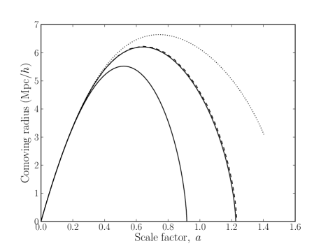
C.0.4 Comparison of methods

The three modified-dynamics methods give very similar results when the deviation from the Newtonian trajectory is small, usually when $R<\lambda$ at all times. However, in more extreme scenarios the Raychaudhuri equation method overstates the degree to which the gravity modification changes the trajectory, in comparison to the inhomogeneous sphere method, which we assume is the most accurate. $R(a)$ trajectories for the three modified gravity solutions are shown in FIG. 9, along with the associated Newtonian path; $\alpha=5$, $\lambda=5\,h^{-1}\,\text{Mpc}$.

It appears that the local approximation inherent in the Raychaudhuri method breaks down when $R\gtrsim\lambda$. However, the homogeneous-sphere approximation continues to hold until well beyond the limits of interest: $M\lesssim 10^{16}\,\mathrm{M_{\odot}/h}$, $\lambda\gtrsim 10\,\,h^{-1}\,\text{Mpc}$.

References

- Creminelli et al. (2009) P. Creminelli, G. D’Amico, J. Norena, and F. Vernizzi, JCAP 0902, 018 (2009), eprint 0811.0827.
- Dvali et al. (2000) G. R. Dvali, G. Gabadadze, and M. Porrati, Phys. Lett. B485, 208 (2000), eprint hep-th/0005016.
- Nicolis et al. (2009) A. Nicolis, R. Rattazzi, and E. Trincherini, Phys. Rev. D79, 064036 (2009), eprint 0811.2197.
- de Rham et al. (2010) C. de Rham, G. Gabadadze, and A. J. Tolley (2010), eprint 1011.1232.
- Fierz (1956) M. Fierz, Helv. Phys. Acta 29, 128 (1956).
- Jordan (1959) P. Jordan, Z. Phys. 157, 112 (1959).
- Brans and Dicke (1961) C. Brans and R. H. Dicke, Phys. Rev. 124, 925 (1961).
- Buchdahl (1970) H. A. Buchdahl, Mon. Not. Roy. Astron. Soc. 150, 1 (1970).
- Carroll et al. (2004) S. M. Carroll, V. Duvvuri, M. Trodden, and M. S. Turner, Phys. Rev. D70, 043528 (2004), eprint astro-ph/0306438.
- Hui and Parfrey (2008) L. Hui and K. P. Parfrey, Phys. Rev. D77, 043527 (2008), eprint 0712.1162.
- Fry (1996) J. N. Fry, Astrophys. J. 461, L65 (1996).
- Tegmark and Peebles (1998) M. Tegmark and P. J. E. Peebles (1998), eprint astro-ph/9804067.
- Press and Schechter (1974) W. H. Press and P. Schechter, Astrophys. J. 187, 425 (1974).
- Bardeen et al. (1986) J. M. Bardeen, J. R. Bond, N. Kaiser, and A. S. Szalay, Astrophys. J. 304, 15 (1986).
- Bond et al. (1991) J. R. Bond, S. Cole, G. Efstathiou, and N. Kaiser, Astrophys. J. 379, 440 (1991).
- Lacey and Cole (1993) C. Lacey and S. Cole, Mon. Not. Roy. Astron. Soc. 262, 627 (1993).
- Sheth (1998) R. K. Sheth, Mon. Not. Roy. Astron. Soc. 300, 1057 (1998), eprint astro-ph/9805319.
- Martino et al. (2009) M. C. Martino, H. F. Stabenau, and R. K. Sheth, Phys. Rev. D79, 084013 (2009), eprint 0812.0200.
- Schmidt et al. (2009) F. Schmidt, M. Lima, H. Oyaizu, and W. Hu, Phys. Rev. D79, 083518 (2009), eprint 0812.0545.
- Khoury and Wyman (2009) J. Khoury and M. Wyman, Phys. Rev. D80, 064023 (2009), eprint 0903.1292.
- Schmidt (2009) F. Schmidt, Phys. Rev. D80, 123003 (2009), eprint 0910.0235.
- Chan and Scoccimarro (2009) K. C. Chan and R. Scoccimarro, Phys. Rev. D80, 104005 (2009), eprint 0906.4548.
- Schmidt et al. (2010) F. Schmidt, W. Hu, and M. Lima, Phys. Rev. D81, 063005 (2010), eprint 0911.5178.
- Sheth and Tormen (1999) R. K. Sheth and G. Tormen, Mon. Not. Roy. Astron. Soc. 308, 119 (1999), eprint astro-ph/9901122.
- Lue et al. (2004) A. Lue, R. Scoccimarro, and G. Starkman, Phys. Rev. D69, 044005 (2004), eprint astro-ph/0307034.
- Dalal et al. (2008) N. Dalal, O. Dore, D. Huterer, and A. Shirokov, Phys. Rev. D77, 123514 (2008), eprint 0710.4560.
- Chandrasekhar (1943) S. Chandrasekhar, Rev. Mod. Phys. 15, 1 (1943).
- Mo and White (1996) H. J. Mo and S. D. M. White, Mon. Not. Roy. Astron. Soc. 282, 347 (1996), eprint astro-ph/9512127.
- Sheth and Lemson (1999) R. K. Sheth and G. Lemson, Mon. Not. Roy. Astron. Soc. 304, 767 (1999), eprint astro-ph/9808138.
- Fry and Gaztanaga (1993) J. N. Fry and E. Gaztanaga, Astrophys. J. 413, 447 (1993), eprint astro-ph/9302009.
- Kitayama and Suto (1996) T. Kitayama and Y. Suto, Astrophys. J. 469, 480 (1996), eprint arXiv:astro-ph/9604141.
- Sheth and Tormen (2002) R. K. Sheth and G. Tormen, Mon. Not. Roy. Astron. Soc. 329, 61 (2002), eprint arXiv:astro-ph/0105113.
- Lam and Sheth (2009) T. Y. Lam and R. K. Sheth, Mon. Not. Roy. Astron. Soc. 398, 2143 (2009), eprint 0905.1702.
- Zhang and Hui (2006) J. Zhang and L. Hui, Astrophys. J. 641, 641 (2006), eprint astro-ph/0508384.
- Press et al. (1992) W. H. Press, S. A. Teukolsky, W. T. Vetterling, and B. P. Flannery, Numerical Recipes in C: The Art of Scientific Computing (Cambridge: University Press, —c1992, 2nd ed., 1992).
- Schaefer and Koyama (2008) B. M. Schaefer and K. Koyama, Mon. Not. Roy. Astron. Soc. 385, 411 (2008), eprint 0711.3129.
- Eisenstein and Hu (1998) D. J. Eisenstein and W. Hu, Astrophys. J. 496, 605 (1998), eprint astro-ph/9709112.
- Komatsu et al. (2009) E. Komatsu, J. Dunkley, M. R. Nolta, C. L. Bennett, B. Gold, G. Hinshaw, N. Jarosik, D. Larson, M. Limon, L. Page, et al., Astrophys. J. Suppl. Ser. 180, 330 (2009), eprint 0803.0547.
- Sheth et al. (2001) R. K. Sheth, H. J. Mo, and G. Tormen, Mon. Not. Roy. Astron. Soc. 323, 1 (2001), eprint astro-ph/9907024.
- Tegmark et al. (2006) M. Tegmark et al., Phys. Rev. D74, 123507 (2006), eprint astro-ph/0608632.
- Masjedi et al. (2008) M. Masjedi, D. W. Hogg, and M. R. Blanton, Astrophys. J. 679, 260 (2008), eprint 0708.3240.
- Wake et al. (2008) D. A. Wake et al. (2008), eprint 0802.4288.
- Desjacques and Sheth (2010) V. Desjacques and R. K. Sheth, Phys. Rev. D81 (2010), eprint 0909.4544.
- Hamaus et al. (2010) N. Hamaus, U. Seljak, V. Desjacques, R. E. Smith, and T. Baldauf, Phys. Rev. D 82, 043515 (2010), eprint 1004.5377.
- Cai et al. (2010) Y. Cai, G. Bernstein, and R. K. Sheth, ArXiv e-prints (2010), eprint 1007.3500.
- Wagoner (1970) R. V. Wagoner, Phys. Rev. D1, 3209 (1970).
- Hui et al. (2009) L. Hui, A. Nicolis, and C. W. Stubbs, Phys. Rev. D 80, 104002 (2009), eprint 0905.2966.
- Hui and Nicolis (2010) L. Hui and A. Nicolis, Phys. Rev. Lett. in press, [arXiv:1009.2520 [hep (2010), eprint 1009.2520.
- Gibbons and Whiting (1981) G. W. Gibbons and B. F. Whiting, Nature (London) 291, 636 (1981).
- Gaztañaga and Lobo (2001) E. Gaztañaga and J. A. Lobo, Astrophys. J. 548, 47 (2001), eprint astro-ph/0003129.