No evidence for anomalously low variance circles on the sky
Abstract
In a recent paper, Gurzadyan & Penrose claim to have found directions on the sky centred on which are circles of anomalously low variance in the cosmic microwave background (CMB). These features are presented as evidence for a particular picture of the very early Universe. We attempted to repeat the analysis of these authors, and we can indeed confirm that such variations do exist in the temperature variance for annuli around points in the data. However, we find that this variation is entirely expected in a sky which contains the usual CMB anisotropies. In other words, properly simulated Gaussian CMB data contain just the sorts of variations claimed. Gurzadyan & Penrose have not found evidence for pre-Big Bang phenomena, but have simply re-discovered that the CMB contains structure.
pacs:
98.80.Bp, 98.80.Es, 95.85.BhA recent preprint by Gurzadyan & Penrose Gurzadyan and Penrose (2010) (hereafter GP10) makes what must be considered by any standard to be an extraordinary claim – that the cosmic microwave background (CMB) contains statistically unusual circles which are signatures of events which happened before the hot, dense stage in the usual Big Bang theory. In particular, GP10 claim to have found directions on the sky centred on which are circles of anomalously low variance in the CMB. If true, this would have profound implications for our understanding of the early Universe, since such features are not expected in the standard picture of primordial structure, based on Gaussian random fields. Such a result would also be very surprising, given the intense scrutiny the CMB has seen in the search for signs of non-Gaussianity. However, we will show that the evidence claimed in GP10 fails to be extraordinary; indeed, such low-variance circles are expected to arise, as properly simulated data show.
GP10 studied maps from the Wilkinson Microwave Anisotropy Probe (WMAP) 7-year data release Jarosik et al. (2011). They specifically looked at circles around particular positions, calculating the variance within annuli of width, and plotting this variance as a function of radius. They found some positions where there appeared to be concentric rings of suppressed variance. In addition, figure 2 in GP10 implies that the scatter in the annulus variances is much larger in some particular locations than it is for a simulated CMB sky.
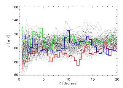
We first tried to reproduce the plots of the variance in annuli presented for the two selected positions in GP10. We found that we could reproduce very similar results (see Fig. 1), and that these are present in both W-band and V-band maps, as well as in the so-called ILC map (see Lam ), which is largely free of foreground signals. Hence it is clear that the particular map used is not the issue, and it is also unlikely that foregrounds are a major part of the effect. Moreover, we found that strong variation among the annuli could be seen all over the map. In other words, the particular positions selected in GP10 did not seem very unusual. Additionally we could find rings of high variance just as easily as those of low variance (examples can be seen in Fig. 1); this is just what would be expected if both low and high variance rings are simply random excursions.

For all of the results presented here we used the masked CMB maps. In each case we choose 500 random directions at Galactic latitudes of . Also, because of the WMAP scanning process, the number of samples going into individual pixels can vary, and so the uncertainty in the temperature varies across the sky. Therefore our results include proper noise weighting and removal of bias. As a check, we also performed the calculations using the unmasked sky, and not taking into account noise weighting. In this case, our results for the two directions chosen in GP10 matched those of GP10 almost perfectly. However, ignoring these details did not have a large effect on our results (despite one of the directions suggested in GP10 being very close to the north ecliptic pole).
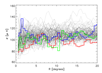
We next turned our attention to simulations. We performed the same variance calculations as described above, but applied to a combination of simulated maps for all W-band feedhorns over the full 7 years (as provided on the LAMBDA website Lam ); this should represent a realistic simulation of the CMB signal plus the WMAP noise. Our results are presented in Fig. 2. Comparing with Fig. 1, it is clear that the expectation of the annulus variances, together with their degree of fluctuation, are indistinguishable between the simulated data and the real data. Since the WMAP data are dominated by the CMB anisotropies rather than by instrumental noise, it is not surprising that we found qualitatively the same results using simpler simulations which were based purely on the estimated power spectrum, Larson et al. (2011), or equivalently the temperature angular correlation function, .
In Fig. 2 we also indicate specific curves which we selected based on the presence of particularly low variance annuli. This demonstrates that the simulated data contain similar low-variance circles as occur in the real data (e.g. the green curve could be claimed to have a ‘family’ of multiple low variance rings). The red curve was also chosen on the basis that it is systematically lower than average, similar to the GP10 , direction. This example was found by searching 500 random directions, as opposed to 10885 in GP10. Hence it is clear that there is nothing unusual about this GP10 direction, and that it is simply an outlier with lower than average variance.
Results for a simulated sky are also presented in GP10 (the third panel of their figure 2), where the fluctuations in the variance appear very small compared with the real data. Details of this simulation are not provided in GP10. However, we found that we could reproduce a similar plot by using purely white noise simulations – i.e. , normalized to have approximately the correct total power. It is clear that the scatter around the average variance level for the GP10 simulation is not what is expected in a map containing the observed CMB anisotropies; instead, it agrees with that for a spectrum with entirely the wrong scale dependence.

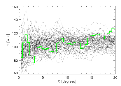
It is important to point out that even when a low-variance annulus is identified in real or simulated data, that does not imply the presence of a circular feature in the map. The low variance could simply be due to particularly low fluctuations in a segment of the annulus. Indeed, it is straightforward to repeat the above analysis, but searching for low-variance features of shapes other than circular annuli. As an example, we performed the identical analysis steps, but looking instead for low-variance ‘triangular annuli’, i.e. the regions between concentric equilateral triangles of different sizes tri . The results are presented in Fig. 3. It is clear from this figure that there are directions around which there are similarly low-variance triangles to the low-variance circles found above. Therefore there is nothing special about the presence of low-variance circles on the sky. We also tested the same triangles in simulated data, finding results consistent with those in Fig. 3.

We have refrained from any attempt to estimate the significance level for the specific patterns identified in GP10. Since the predictions for low variance annuli are quite vague, it would be impossible to avoid the issue of a posteriori statistics. But in any case, this is unnecessary, since it is clear that such low variance patterns occur by chance in realistically simulated skies.
Recalling that the CMB ‘signal’ behaves statistically like a random ‘noise’, and that it is Gaussian in nature, it is possible to understand theoretically the behaviour of the variances in the annuli. All that is required is the power spectrum, or its real-space equivalent, the 2-point angular correlation function, which is essentially the variance on the sky as a function of angular separation between positions. The variance of the temperature within an annulus, where labels the pixel, is
| (1) |
where is the number of pixels. This is the variance for one particular realization of the Gaussian random field. Taking the expectation over all realizations in the ensemble (denoted ) gives
| (2) |
where
| (3) |
In the limit of large , we have , i.e. the expected variance is independent of the shape of the region, and is given simply by the zero-lag angular correlation function . This is around , which we estimate from the actual WMAP W-band map, which includes noise. This matches the levels seen in Figs. 1–3 for large .
Now we want the variance of over the ensemble. So we want
| (4) |
Straightforward computations give
| (5) | |||||
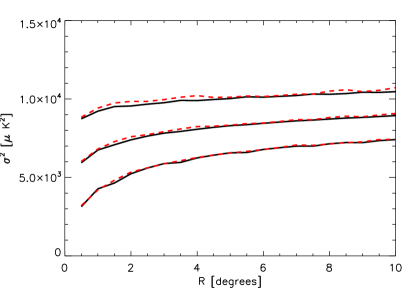
In Fig. 4 we show the theoretical values for the expectation and variance of the annulus variance in Eqs. (2) and (5), compared to simulations based on a noiseless full-sky map from the best-fit WMAP 7-year power spectrum Larson et al. (2011), convolved with a Gaussian beam (which is close to the W-band beam size). We use only the CMB component for simplicity, since the ensemble average power spectrum (required to compute the theoretical values) is known in advance (whereas the actual W-band map also contains noise and a foreground component). This is why in Fig. 4 is slightly below the levels in the previous figures. Note that Figs. 1–3 plot the standard deviation, , to enable direct comparison with GP10, while Fig. 4 plots the variance, . This is because the above derivation does not carry over straightforwardly to the standard deviation.
We see that the theoretical values agree very well with the results of actual calculations of the variance for many centres. The suppression in variance observed for small is simply due to the presence of structures in the CMB on the prefered scale of the first acoustic peak at : the smallest annuli are roughly this size, and hence the temperature is expected to be more strongly correlated, i.e. the variances lower, than for annuli with larger .

In summary, the CMB probes the largest accessible scales, and so it is certainly worth looking for signatures which may be smoking guns for new physics (from the extensive literature on this topic, we randomly suggest Moss et al. (2010)). Such signatures certainly could reveal information about the earliest stages of the Universe. We have confirmed the presence of the low-variance circles in the CMB sky found by GP10. However, we have shown that such circles are to be expected in typical realizations of the CMB sky based on the usual assumption of Gaussian random primordial fluctuations with the scale dependence which is now so well measured. So if there are signals of extraordinarily early times buried in the CMB, they have not yet been found, and we will have to keep looking.
Acknowledgments.—This research was supported by the Natural Sciences and Engineering Research Council of Canada and the Canadian Space Agency. We thank Andrei Frolov and Jonathan Benjamin for useful discussions. Use was made of the HEALPix Gorski et al. (2005) software package. After this study was completed we became aware of two other papers Wehus and Eriksen (2010); Hajian (2010) which come to essentially identical conclusions.
References
- Gurzadyan and Penrose (2010) V. G. Gurzadyan and R. Penrose (2010), arXiv:1011.3706 [astro-ph.CO].
- Jarosik et al. (2011) N. Jarosik et al., Astrophys. J. Suppl. 192, 14 (2011), arXiv:1001.4744[astro-ph.CO].
- (3) http://lambda.gsfc.nasa.gov/.
- Larson et al. (2011) D. Larson et al., Astrophys. J. Suppl. 192, 16 (2011), arXiv:1001.4635[astro-ph.CO].
- (5) One could instead imagine searching for other shapes, even special shapes which tile the sphere.
- Moss et al. (2010) A. Moss, D. Scott, J. P. Zibin, and R. Battye (2010), arXiv:1011.2990 [astro-ph.CO].
- Gorski et al. (2005) K. M. Gorski et al., Astrophys. J. 622, 759 (2005), arXiv:astro-ph/0409513.
- Wehus and Eriksen (2010) I. K. Wehus and H. K. Eriksen (2010), arXiv:1012.1268 [astro-ph.CO].
- Hajian (2010) A. Hajian (2010), arXiv:1012.1656 [astro-ph.CO].