Spin Susceptibility and Helical Magnetic Orders at the Edges/Surfaces of Topological Insulators Due to Fermi Surface Nesting

Abstract

We study spin susceptibility and magnetic order at the edges/surfaces of two-dimensional and three-dimensional topological insulators when the Fermi surface is nested. We find that due to spin-momentum locking as well as time-reversal symmetry, spin susceptibility at the nesting wavevector has a strong helical feature. It follows then, a helical spin density wave (SDW) state emerges at low temperature due to Fermi surface nesting. The helical feature of spin susceptibility also has profound impact on the magnetic order in magnetically doped surface of three dimensional topological insulators. In such system, from the mean field Zener theory, we predict a helical magnetic order.

I Introduction

In the past few years, a new family of materials called topological insulators (TIs) have been theoretically predicted KaneMele2 ; BHZ ; FuKaneMele ; FuKane ; MooreBalents ; Roy and then experimentally observed.Konig ; Hsieh ; Xia ; YLChen A TI has a energy gap in the bulk and gapless excitation in the edge/surface, which is due to the nontrivial band topology and protected by time reversal symmetry. TIs possess a nontrivial topological order, which distinguishes them from simple band insulators. In a two dimensional (2D) TI, which is also known as a quantum spin Hall insulator, the edge states form a helical Luttinger liquid.WuBernevigZhang The surface states of three dimensional (3D) TIs form a “helical metal” with Dirac cone like spectrum FuKaneMele ; FuKane ; Zhang ; Hsieh ; Xia ; Hsieh2 ; FFT-STM (Specifically, in this paper, we are interested in a class of 3D TIs where the surface state consists of a single Dirac cone. Examples are Bi₂Te₃,Zhang ; YLChen Bi₂Se₃,Zhang ; Xia ; Kuroda Sb₂Te₃,Zhang ; Hsieh3 TlBiSe₂Kuroda2 ; TlBiSe , and many other materialsTlBiTe ; SYXu . Due to large bandgap and high purity, these materials have great potential for application and scientific research.HasanKane ). An important feature is that spin and momentum are closely correlated in the edge/surface states of TIs, which leads to many unusual effectsDai ; GV ; HasanKane ; Qireview and potential applications in spintronics and quantum computation.spintronics

Recently, it was found in Bi₂Te₃ that the as Fermi energy increases from the Dirac point, the shape of Fermi surface gradually changes from a circle, first to a hexagonal shape, and then to a snowflake-like.YLChen ; Alpich This phenomenon was also found in other 3D TIs with similar structures.Kuroda ; Hsieh3 ; TlBiSe ; TlBiTe ; SYXu This kind of band structure is theoretically reproduced by Fu from the $k\cdot p$ theory.Fu For a certain range of energies, the Fermi surface is almost a hexagon, which leads to strong nesting at three wavevectors and possible instability to the formation of SDW states.Fu

In this paper, we study spin susceptibility and magnetic order at the edges/surfaces of TIs when the Fermi surface is nested. We find that due to the one-to-one correspondence between spin state and momentum (“spin-momentum locking”) as well as time reversal symmetry, the spin susceptibility function at nesting wavevector has a strong helical feature. It follows then, a helical SDW state emerges at low temperature due to Fermi surface nesting. We present a mean field theory of the helical SDW state. The helical feature of the spin susceptibility function also has profound impact on the magnetic order in the magnetically doped surfaces of 3D TIs. In such system, from the mean field Zener theory, we predict a helical magnetic order.

II Hamiltonian, spectrum and eigenstates

We consider the situation where Fermi surface exhibits strong nesting feature. Examples are, the edge states in a 2D TI, and the surface state in the 3D TI Bi₂Te₃ with Fermi energy in the range of [0.13, 0.23] eV where the Fermi surface is almost a hexagon YLChen ; Fu [see Fig. 1]. The hexagonal shape of Fermi surface also exists in the surface states of many other 3D TIs, such as Bi₂Se₃,Liu ; Kuroda Sb₂Te₃,Fu ; Liu TlBiSe₂Kuroda2 ; TlBiSe , TlBiTe₂TlBiTe and a recently discovered large class of 3D TIs in Ref. SYXu, . In the following we would call these materials the “Bi₂Se₃ class”.

The Hamiltonian of the edge states in a 2D TI can be written asWuBernevigZhang

$$H_{0}=\sum_{k\alpha\beta}v_{0}k~{}c^{\dagger}_{k\alpha}\sigma^{z}_{\alpha\beta}c_{k\beta},$$ (1)

where $v_{0}$ is the Fermi velocity. The spin orientations of the eigenstates, through proper choosing of the spin coordinates, have been taken as up and down. The eigenenergies and eigenstates are

$$\varepsilon_{\pm}(k)=\pm v_{0}|k|,\quad u_{\pm}(k)=\left(\begin{array}[]{c}\Theta(\pm k)\\ \Theta(\mp k)\end{array}\right),$$ (2)

where $\Theta$ is the Heaviside function. The nesting vector is $Q=2k_{F}$.

Throughout this paper, we focus on the situation where the Fermi energy $E_{F}$ is high and the temperature is low, so that states far below the Fermi surface (such as those below the Dirac point) is irrelevant. This regime is easy to achieve in the Bi₂Se₃ class of 3D TIs, thanks to the large bandgap and Dirac velocity.

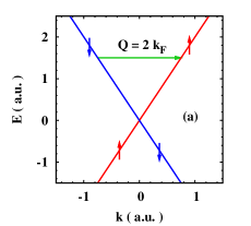
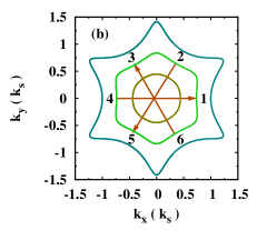
Figure 1: (Color online) (a) Spectrum of the edge states of 2D TIs as well as schematic of the nesting wave-vector $Q=2k_{F}$. Nesting wavevector connects spin-down and spin-up states. (b) Energy contour of the surface states of 3D TIs for three typical energy, $0.2,0.7,2$ $E_{s}$, as well as schematic of nesting wave-vectors for hexagonal Fermi surface. The numbers label the Fermi Arcs. There are three nesting wavevectors, ${\bf Q}_{1}$ from Arc 4 to Arc 1, ${\bf Q}_{2}$ from Arc 6 to Arc 3, ${\bf Q}_{3}$ from Arc 2 to Arc 5.

The Hamiltonian for the surface states in 3D TI with a single Dirac cone, is given in Refs. Fu, ; Liu, . Keeping only the dominant terms, the Hamiltonian is (with $x$ and $y$ axes along the $\Gamma-K$ and $\Gamma-M$ directions respectively),Fu ; Liu

$$H_{0}=v(k_{x}\sigma_{y}-k_{y}\sigma_{x})+\frac{\gamma}{2}(k_{+}^{3}+k_{-}^{3})\sigma_{z},$$ (3)

where $k_{\pm}=k_{x}\pm{\rm i}k_{y}$. The eigenenergy and spin states areLiu

$$\varepsilon_{\pm}({\bf k}) = \pm\sqrt{v^{2}k^{2}+\gamma^{2}k^{6}\cos^{2}3\theta_{k}},$$ (4)

$$u_{\pm}({\bf k}) = \frac{1}{\sqrt{A({\bf k})}}\left(\begin{array}[]{c}vk(\sin\theta_{k}+{\rm i}\cos\theta_{k})\\ \varepsilon_{\pm}({\bf k})-\gamma k^{3}\cos 3\theta_{k}\end{array}\right),$$ (7)

with ${\bf k}=k(\cos\theta_{k},\sin\theta_{k})$, $A({\bf k})=v^{2}k^{2}+(\varepsilon_{+}({\bf k})-\gamma k^{3}\cos 3\theta_{k})^{2}$. The Hamiltonian is time-reversal invariant. The last term reduces the symmetry from $C_{\infty v}$ to $C_{3v}$. The Hamiltonian describes the surface state of the Bi₂Se₃ class of 3D TIs.Fu ; Liu It is instructive to rescale the Hamiltonian with,Fu

$$H_{0}=E_{s}H_{0}^{\prime},\quad k=k_{s}k^{\prime},$$ (8)

where

$$E_{s}=v\sqrt{v/\gamma},\quad k_{s}=\sqrt{v/\gamma}.$$ (9)

Then the Hamiltonian becomes

$$H_{0}^{\prime}=(k_{x}^{\prime}\sigma_{y}-k_{y}^{\prime}\sigma_{x})+\frac{1}{2}(k_{+}^{\prime 3}+k_{-}^{\prime 3})\sigma_{z}.$$ (10)

Obviously, the physical properties are universal in these materials, with exact quantitative scaling by properly recovering the dimension via $E_{s}$ and $k_{s}$ within the above model. The parameters, $v$, $\gamma$, $E_{s}$ and $k_{s}$ of several 3D TIs inferred from experiments are listed in Table I.

Table 1: Hamiltonian parameters of the surface states in 3D TIs with hexagonal symmetry. (^a from Ref. Fu, , ^b from Ref. Kuroda, , ^c inferred from Ref. TlBiSe, , ^d inferred from Ref. SYXu, .)

		$v$ (eVÅ)		$\gamma$ (eVÅ3)		$E_{s}$ (eV)		$k_{s}$ (Å-1)
Bi2Te3a:		2.55		250		0.26		0.1
Bi2Se3b:		3.55		128		0.59		0.17
TlBiSe2c:		3.1		182		0.4		0.13
GeBi2Te4d:		2.37		99		0.37		0.15
Bi2Te2Sed:		7.25		580		0.81		0.11

If the Fermi energy is in the range of $0.5E_{s}\leq E_{F}\leq 0.9E_{s}$, the Fermi surface is almost a hexagon, which exhibits strong nesting feature.Fu There are three nesting wave-vectors

$${\bf Q}_{1} = 2k_{0}(1,0),\quad\quad{\bf Q}_{2}=2k_{0}(-\frac{1}{2},\frac{\sqrt{3}}{2}),$$

$$\quad\quad{\bf Q}_{3} = 2k_{0}(-\frac{1}{2},-\frac{\sqrt{3}}{2}),$$ (11)

where $k_{0}$ is determined by $\sqrt{v^{2}k_{0}^{2}+\gamma^{2}k_{0}^{6}}=E_{F}$.

At higher Fermi energy, the Fermi surface is distorted to snowflake-like and new nesting wave-vectors emerges.Fu ; Alpich However, at such high Fermi energy usually the bulk conduction band is also occupied, which complicates the situation and is not interested in this paper.

The electron-electron interaction consists of the long-range Coulomb interaction and the short-range Hubbard interaction. The former does not affect the spin susceptibility [to the random phase approximation (RPA)note0 ] and is hence ignored. The onsite Hubbard interaction is written as

$$H_{U} = -\frac{U}{3}\sum_{{\bf q}}\mbox{\boldmath$\sigma$\unboldmath}({\bf q})\cdot\mbox{\boldmath$\sigma$\unboldmath}({\bf-q}),$$ (12)

where $\mbox{\boldmath$\sigma$\unboldmath}({\bf q})=\sum_{{\bf k}\alpha\beta}c^{\dagger}_{{\bf k}\alpha}\mbox{\boldmath$\sigma$\unboldmath}_{\alpha\beta}c_{{\bf k}+{\bf q}\beta}$ with $\sigma$ being Pauli matrices vector and $\alpha,\beta$ being spin indices. For positive Hubbard $U$ (repulsive interaction), Fermi surface nesting leads to the SDW instability and transition into the SDW state at sufficient low temperature. Whereas, for negative $U$ (attractive interaction), it leads to the charge density wave (CDW) instability and the emergence of CDW state. Here we assume, as in most cases, $U>0$.

III Spin susceptibility and SDW instability

III.1 Edge states of 2D TIs

The linear spin susceptibility function is

$$\chi_{\mu\nu}(q,\omega)={\rm i}\int_{0}^{\infty}dt\langle[\sigma_{\mu}(q,t),\sigma_{\nu}(-q,0)]\rangle e^{{\rm i}t(\omega+{\rm i}0^{+})},$$ (13)

where $\mu,\nu=(x,y,z)$ or $(\pm,z)$ with $\sigma_{\pm}=\frac{1}{2}(\sigma_{x}\pm{\rm i}\sigma_{y})$. In the edge of a 2D TI, at the nesting vector $Q=2k_{F}$, the only nonzero terms are $\chi_{+-}(-Q,\omega)$ and $\chi_{-+}(Q,\omega)$ as the nesting wavevector connects spin-down and spin-up states. This helical feature of the spin susceptibility function is due to spin-momentum locking as well as time reversal symmetry. The two susceptibility function are actually related by $[\chi_{+-}(-Q,-\omega)]^{\ast}=\chi_{-+}(Q,\omega)$. In the absence of interaction, the spin susceptibility is

$$\chi^{0}_{-+}(Q,\omega)=\sum_{k}\frac{n_{F}(\xi_{k+Q\uparrow})-n_{F}(\xi_{k\downarrow})}{\omega-\xi_{k+Q\uparrow}+\xi_{k\downarrow}+i0^{+}},$$ (14)

where $\xi_{k\downarrow}=\varepsilon_{k\downarrow}-E_{F}$ and $n_{F}$ is the Fermi distribution. Including the Hubbard interaction within RPA, one gets

$$\chi_{-+}(Q,\omega)=\frac{\chi^{0}_{-+}(Q,\omega)}{1-U\chi^{0}_{-+}(Q,\omega)}.$$ (15)

Due to Fermi surface nesting, the spin susceptibility $\chi^{0}_{-+}(Q,0)$ is divergent at low temperature. Actually, directly from Eq. (14), one can show that $\chi^{0}_{-+}(Q,0)\approx\frac{1}{\pi v}\log(E_{F}/k_{B}T)$. That is, the spin susceptibility function is logarithmically divergent with decreasing temperature. This signals the SDW instability. The feature that only $\chi^{0}_{-+}(Q,0)$ diverges indicates a helical SDW order.

The above treatment based on the Fermi-liquid theory is of course invalid for one-dimensional electron system, but it sheds some light on the problem. In the following, we analyze the problem via the bosonization theory.

Following Wu et al., WuBernevigZhang the bosonized Hamiltonian in the presence of Umklapp scattering can be expressed as

$$H = \frac{1}{2\pi}\int dx\left[uK\left(\nabla\theta(x)\right)^{2}+\frac{u}{K}\left(\nabla\phi(x)\right)^{2}\right]$$ (16)

$$\mbox{}~{}~{}+\frac{g_{u}}{2(\pi a)^{2}}\cos(4\phi(x)),$$

where the bosonized fermion fields are

$$\psi_{R\uparrow}(x)=\frac{e^{ik_{F}x}}{\sqrt{2\pi a}}e^{-i\phi_{R}(x)},\quad\psi_{L\downarrow}(x)=\frac{e^{-ik_{F}x}}{\sqrt{2\pi a}}e^{i\phi_{L}(x)},$$ (17)

with $\phi=(\phi_{R}+\phi_{L})/2$, $\theta=(\phi_{R}-\phi_{L})/2$. $K$ the Luttinger parameter. $u$ is the renormalized Fermi velocity. $g_{u}$ is the Umklapp scattering strength. $a$ is a short-distance cutoff. Due to symmetry reasons, the only possible instabilities are SDW and singlet superconductivity (SC). This is because CDW and triplet SC instabilities pair particles with the same spin, i.e., terms like $\psi_{R\uparrow}^{\dagger}\psi_{L\uparrow}$ for CDW and $\psi_{R\uparrow}^{\dagger}\psi_{L\uparrow}^{\dagger}$ for triplet SC, are impossible. The bosonized form of spin operators are

$$\sigma_{+}(x)=\psi_{R\uparrow}^{\dagger}(x)\psi_{L\downarrow}(x)=\frac{e^{-i2k_{F}x}}{2\pi a}e^{2i\phi(x)},$$

$$\sigma_{-}(x)=\psi_{L\downarrow}^{\dagger}(x)\psi_{R\uparrow}(x)=\frac{e^{i2k_{F}x}}{2\pi a}e^{-2i\phi(x)}.$$ (18)

From standard bosonization theory, Giamarchi the Umklapp term becomes relevant when $K<1/2$. Then RG flow will go to a strong coupling fixed point, $g_{u}\rightarrow\infty$, and the $\phi$ field will become ordered. Depending on the sign of $g_{u}$, the ordered value of $\phi$ is

$$\langle\phi\rangle = \frac{\pi}{4}+\frac{2n\pi}{4},\ \ \ \ \ g_{u}>0,$$

$$\langle\phi\rangle = 0+\frac{2n\pi}{4},\ \ \ \ \ \ g_{u}<0.$$ (19)

This signifies a true phase transition. Then the spin operators, which have zero expectation values in the non ordered phase, also acquire nonzero average value across the transition,

$$\langle\sigma_{x}\rangle = \langle\sigma_{+}+\sigma_{-}\rangle=\frac{2}{(2\pi a)^{2}}\cos(2k_{F}x-\langle\phi\rangle),$$

$$\langle\sigma_{y}\rangle = \frac{1}{i}\langle\sigma_{+}-\sigma_{-}\rangle=\frac{-2}{(2\pi a)^{2}}\sin(2k_{F}x-\langle\phi\rangle),$$ (20)

which shows helical structure and is consistent with the mean field result. We note that very recently a similar calculation has been carried out by Kharitonov,Kharitonov considering helical Luttinger liquid in the proximity to a ferromagnet, which also agrees with our result.

III.2 Surface states of 3D TIs

General considerations

On the surface of a 3D TI, the nesting vector will connect states which are not Kramers pairs and hence their spin states are not antiparallel. As a consequence, the spin susceptibility is finite in all directions. The free spin susceptibility function in this case is

$$\chi^{0}_{\mu\nu}({\bf Q},0)=\sum_{\bf k}\frac{n_{F}(\xi_{{\bf k+Q}+})-n_{F}(\xi_{{\bf k}+})}{\xi_{{\bf k}+}-\xi_{{\bf k+Q}+}+i0^{+}}g_{\mu}({\bf k},{\bf Q})g^{\ast}_{\nu}({\bf k},{\bf Q})$$ (21)

where

$$g_{\mu}({\bf k},{\bf Q})=\langle u_{+}({\bf k})|\sigma_{\mu}|u_{+}({\bf k+Q})\rangle$$ (22)

with $\mu,\nu=(x,y,z)$. One can note that, $g_{\mu}({\bf k},{\bf Q})g^{\ast}_{\nu}({\bf k},{\bf Q})$ is a bilinear tensor, where $g_{\mu}({\bf k},{\bf Q})$ is its eigenvector with eigen-value

$$\kappa_{g}({\bf k},{\bf Q})=\sum_{\mu}|g_{\mu}({\bf k},{\bf Q})|^{2}.$$ (23)

Moreover, if

$$g_{0}({\bf k},{\bf Q})=\langle u_{+}({\bf k})|u_{+}({\bf k+Q})\rangle,$$ (24)

and

$$\chi^{0}_{c}({\bf Q},0)=\sum_{\bf k}\frac{n_{F}(\xi_{{\bf k+Q}+})-n_{F}(\xi_{{\bf k}+})}{\xi_{{\bf k}+}-\xi_{{\bf k+Q}+}+i0^{+}}|g_{0}({\bf k},{\bf Q})|^{2},$$ (25)

is the charge susceptibility, then

$$|g_{0}|^{2}+\kappa_{g}({\bf k},{\bf Q})\equiv 2,\quad 1\leq\kappa_{g}({\bf k},{\bf Q})\leq 2.$$ (26)

and a “complementary relation” between the spin- and charge- susceptibility,

$$\sum_{\mu}\chi^{0}_{\mu\mu}({\bf Q},0)+\chi^{0}_{c}({\bf Q},0)=\chi^{0}({\bf Q},0)$$ (27)

with $\chi^{0}({\bf Q},0)\equiv\sum_{\bf k}\frac{n_{F}(\xi_{{\bf k+Q}+})-n_{F}(\xi_{{\bf k}+})}{\xi_{{\bf k}+}-\xi_{{\bf k+Q}+}+i0^{+}}$, due to spin-momentum locking. We then introduce the spin density operator

$$\sigma_{g}({\bf k},{\bf Q})=\frac{1}{\kappa_{g}({\bf k},{\bf Q})}\sum_{\mu,\alpha\beta}g_{\mu}^{\ast}({\bf k},{\bf Q})c^{\dagger}_{{\bf k}\alpha}\sigma_{\mu}^{\alpha\beta}c_{{\bf k}+{\bf Q}\beta}.$$ (28)

One can show that

$$\langle u_{+}({\bf k})|\sigma_{g}({\bf k},{\bf Q})|u_{+}({\bf k+Q})\rangle=1.$$ (29)

And, any spin density operator

$$\sigma_{f}({\bf k},{\bf Q})=\sum_{\mu,\alpha\beta}f_{\mu}^{\ast}({\bf k})c^{\dagger}_{{\bf k}\alpha}\sigma_{\mu}c_{{\bf k}+{\bf Q}\beta},$$ (30)

which is perpendicular to $\sigma_{g}$, i.e., $\sum_{\mu}g_{\mu}^{\ast}({\bf k})f_{\mu}({\bf k})=0$, has

$$\langle u_{+}({\bf k})|\sigma_{f}({\bf k},{\bf Q})|u_{+}({\bf k+Q})\rangle=0.$$ (31)

Therefore, only one spin density susceptibility is nonzero (if only ${\bf k}$ and ${\bf k}+{\bf Q}$ states are concerned), which is defined by $\sigma_{g}({\bf k},{\bf Q})$. This intriguing feature is due to spin-momentum locking.

Helical feature

Consider, if ${\bf k}$ and ${\bf k}+{\bf Q}$ are time reversal pair states, of which spin orientations are opposite, the spin density operator $\sigma_{g}({\bf k},{\bf Q})$ is helical, as we learn from the case in the edges of 2D TIs. Unfortunately, here $g_{\mu}({\bf k},{\bf Q})$ is ${\bf k}$ dependent. Besides, only for some very special ${\bf k}$ states, such as ${\bf k}_{0}=(-k_{0},0)$ and ${\bf k}_{0}+{\bf Q}_{1}=(k_{0},0)$, the two states are time reversal pairs. If the contributions of all ${\bf k}$ states are summed, the helical feature may be smeared out.

To study this case, we calculate the free spin susceptibility function $\chi_{\mu\nu}^{0}({\bf Q_{1}},0)$ numerically for $E_{F}\in[0.5,0.9]$ $E_{s}$ where the Fermi surface is hexagonal (${\bf Q}_{1}=(2k_{0},0)$ [see Eq. (11)] connects Fermi Arc 4 and Arc 1 [see Fig. 1(b)]). Our results are presented in Fig. 2. From the calculation, we find that, though the exact helical spin susceptibility is ruled out, the spin susceptibility function still has strong helical feature. Specifically, one of the eigenvalues of the spin susceptibility tensor $\chi_{\mu\nu}^{0}({\bf Q_{1}},0)$ is much larger than the other two [Fig. 2(b)], which corresponds to a spin density response with helicity very close to unity [Fig. 2(c)]. The helical spin rotating axis is indicated in Fig. 2(a) as ${\bf n}_{g}$, which lies in the $y$-$z$ plane with an angle $\theta_{n}$ [Fig. 2(c)] between $y$-axis.

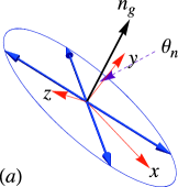
Figure 2: (Color online) (a) Schematic of the spin density response corresponding to the largest eigen-value of the spin susceptibility tensor $\hat{\chi}^{0}({\bf Q}_{1},0)$. ${\bf n}_{g}$ is the helical rotating axis. The blue arrows indicate spins rotating around the ${\bf n}_{g}$ axis. ${\bf n}_{g}$ lies in the $y$-$z$ plane with an angle $\theta_{n}$ between $y$ axis. (b) Eigenvalues (positive definite) of the tensor $\hat{\chi}^{0}({\bf Q}_{1},0)$ as function of Fermi energy (in unit of $E_{s}$). (c) The helicity and the angle $\theta_{n}$ as function of Fermi energy. All data are calculated at $k_{B}T=1.3\times 10^{-3}E_{s}$.

Physical explanations

To understand the above results, let’s consider the problem that how the spin susceptibility function gets maximized at ${\bf Q}_{1}$. The spin susceptibility function for an arbitrary spin density operator, $\sigma_{f}({\bf Q}_{1})=\sum_{\mu}f_{\mu}^{\ast}\sigma_{\mu}({\bf Q}_{1})$ [$\sum_{\mu}|f_{\mu}|^{2}=1$ (normalized), and $\sigma_{\mu}({\bf Q}_{1})=\sum_{{\bf k},\alpha\beta}c^{\dagger}_{{\bf k}\alpha}\sigma_{\mu}^{\alpha\beta}c_{{\bf k}+{\bf Q}_{1}\beta}$], is

$$\chi^{0}_{f}({\bf Q}_{1},0)=\sum_{\bf k}\frac{n_{F}(\xi_{{\bf k}+})-n_{F}(\xi_{{\bf k+Q}_{1}+})}{\xi_{{\bf k+Q}_{1}+}-\xi_{{\bf k}+}}$$

$$\times\Big{|}\sum_{\mu}f_{\mu}^{\ast}\frac{g_{\mu}({\bf k},{\bf Q}_{1})}{\sqrt{\kappa_{g}({\bf k},{\bf Q}_{1})}}\Big{|}^{2}\kappa_{g}({\bf k},{\bf Q}_{1}),$$ (32)

The spin susceptibility gets contribution mainly from the states satisfying the nesting condition and from the vicinity. The above equation also indicates that the contribution is proportional to the factor $\kappa_{g}({\bf k},{\bf Q}_{1})$. It is easy to show that for the special wavevector ${\bf k}_{0}=(-k_{0},0)$, the nesting condition is exactly satisfied, $\xi_{{\bf k}_{0}+}=\xi_{{\bf k}_{0}+{\bf Q}_{1}+}=0$. Moreover, from (denote $g^{0}_{\mu}\equiv g_{\mu}({\bf k}_{0},{\bf Q}_{1})$),

$$g^{0}_{x}={\rm i},\quad g^{0}_{y}=\frac{-\gamma k_{0}^{3}}{\sqrt{v^{2}k_{0}^{2}+\gamma^{2}k_{0}^{6}}},\quad g^{0}_{z}=\frac{-vk_{0}}{\sqrt{v^{2}k_{0}^{2}+\gamma^{2}k_{0}^{6}}},$$ (33)

one finds that the magnitude $\kappa_{g}({\bf k},{\bf Q}_{1})$ is largest at ${\bf k}_{0}=(-k_{0},0)$ with $\kappa_{g}({\bf k}_{0},{\bf Q}_{1})=2$. As ${\bf k}_{0}$ is at the center of the Fermi Arc 4, where the main contribution to spin susceptibility comes, the overlapping factor $\Big{|}\sum_{\mu}f_{\mu}^{\ast}\frac{g_{\mu}({\bf k},{\bf Q}_{1})}{\sqrt{\kappa_{g}({\bf k},{\bf Q}_{1})}}\Big{|}^{2}$ is also very large, if $f_{\mu}^{\ast}=g^{0\ast}_{\mu}/\sqrt{\kappa_{g}({\bf k}_{0},{\bf Q}_{1})}$. Calculation indicates that the overlapping factor is very close to unity in the vicinity of Fermi Arc 4. Therefore, the spin density operator $\sigma_{f}$ which maximizes the spin susceptibility function should be $\sigma_{g}^{0}({\bf Q}_{1})=\sum_{\mu}g^{0\ast}_{\mu}\sigma_{\mu}({\bf Q}_{1})/\sqrt{\kappa_{g}({\bf k}_{0},{\bf Q}_{1})}$. This observation is very close to the truth, except that it ignores some delicate part. Although the factor $\frac{n_{F}(\xi_{{\bf k}+})-n_{F}(\xi_{{\bf k+Q}_{1}+})}{\xi_{{\bf k+Q}_{1}+}-\xi_{{\bf k}+}}$ is peaked at ${\bf k}_{0}=(-k_{0},0)$ (as $\xi_{{\bf k}_{0}+}=\xi_{{\bf k}_{0}+{\bf Q}_{1}+}=0$), the dispersion, however, is asymmetric around ${\bf k}_{0}$ along the $k_{x}$ direction, as the spectrum is nonlinear [see Eq. (4) and Fig. 1]. Therefore, the spin density operator which maximize the spin susceptibility, denoted as $\sigma_{G}$, deviates slightly from $\sigma_{g}^{0}$. Nevertheless, $\sigma_{G}$ is very close to $\sigma_{g}^{0}$ and keeps most of the features of $\sigma_{g}^{0}$, especially the helical feature. This feature even persists to room temperature, thanks to the large bandgap and Dirac velocity in the Bi₂Se₃ class of 3D TIs.

One can write $\sigma_{G}({\bf Q}_{1})=\sum_{\mu}G_{1\mu}^{\ast}\sigma_{\mu}({\bf Q}_{1})$, where

$$G_{1\mu}\approx\frac{1}{\sqrt{2}}g^{0}_{\mu}~{}~{},\quad\quad\sum_{\mu}|G_{1\mu}|^{2}=1~{}.$$ (34)

From Eq. (33), we know that $G_{1x}$ is a pure imaginary number, whereas $G_{1y}$ and $G_{1z}$ are real numbers. Also, $iG_{1x},G_{1y},G_{1z}<0$. Hence the helical spin rotation axis is

$${\bf n}_{g}=(0,\cos\theta_{n},\sin\theta_{n})$$ (35)

with $\theta_{n}={\rm Arctan}(G_{1z}/G_{1y})-\pi/2$, agreeing with the results in Fig. 2. The helicity is $2\sqrt{G_{1y}^{2}+G_{1z}^{2}}|G_{1x}|$. From Eqs. (34) and (33), one can see that the helicity is indeed close to unity.

Systematic results

In Fig. 3(a), we plot the largest eigenvalue of the spin susceptibility tensor, $\chi_{G}^{0}({\bf Q},0)$, as function of $|{\bf Q}|$ with ${\bf Q}$ along the $x$-direction. It is seen that the spin susceptibility function has a strong peak at the nesting wave-vector ${\bf Q}_{1}$, especially when $E_{F}=0.7E_{s}$ where the Fermi surface is almost a perfect hexagon. We also plot the spin susceptibility function at a higher temperature $T=100$ K (blue dotted curve) with chemical potential $0.7E_{s}$. We find that the nesting and the helical features persist to high temperature. And the largest eigenvalue of the spin susceptibility tensor is still much larger than the other two for ${\bf Q}\sim{\bf Q}_{1}$, at high temperature.

We present a two-dimensional plot of $\chi_{G}^{0}({\bf Q},0)$ in Fig. 3(b). It is seen that the spin susceptibility function peaks at regions close to the nesting wavevectors $\pm{\bf Q}_{i}$ $i=(1,2,3)$. Spin susceptibility is small at both small and large ${\bf Q}$. This is quite different from the situation in a normal two-dimensional electron system, where spin susceptibility at small ${\bf Q}$ is large.

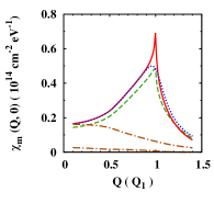
Figure 3: (Color online) (a) The largest eigenvalue of spin susceptibility tensor, $\chi_{G}^{0}({\bf Q},0)$, as function of the wave-vector ${\bf Q}=(Q,0)$ along $x$-direction. Note that $Q$ is in unit of the nesting wavevector $Q_{1}=|{\bf Q}_{1}|=2k_{0}$. The red full (green dashed) curve correspond to the case with $E_{F}=0.7E_{s}$ ($0.5E_{s}$) and temperature $T=4$ K. The blue dotted curve corresponding to the case with chemical potential $0.7$ $E_{s}$ and $T=100$ K. The dot-dashed curves denote other two eigen-values of $\hat{\chi}^{0}$ for the $T=100$ K case. The parameters of Bi₂Te₃ [see Table I] are used.Fu (b) $\chi_{G}^{0}({\bf Q},0)$ as function of ${\bf Q}$ for $E_{F}=0.7E_{s}$, $k_{B}T=1.3\times 10^{-3}E_{s}$. $\chi_{G}^{0}$ is in unit of $0.05(k_{s}^{2}/E_{s})$.

Interaction correction

Then by including the Hubbard interaction within the RPA approximation, one gets

$$\chi_{G}({\bf Q}_{1},0)=\frac{\chi_{G}^{0}({\bf Q}_{1},0)}{1-a_{G}U\chi_{G}^{0}({\bf Q}_{1},0)}.$$ (36)

Here

$$\chi_{G}({\bf Q}_{1},0)={\rm i}\int_{0}^{\infty}dt\langle[\sigma_{G}({\bf Q}_{1},t),(\sigma_{G}({\bf Q}_{1},0))^{\dagger}]\rangle e^{{\rm i}t(0+{\rm i}0^{+})}.$$ (37)

$$a_{G}=\frac{1}{2}\Big{[}1+\big{|}\sum_{\mu}G_{1\mu}^{2}\big{|}^{2}\Big{]},\quad\frac{1}{2}\leq a_{G}\leq 1.$$ (38)

Here the awkward factor $a_{G}$ is due to the factor that the spin density $\sigma_{G}({\bf Q}_{1})$ is not properly normalized. The normalized spin density is

$$\tilde{\sigma}_{G}({\bf Q}_{1})=\sqrt{a_{G}}\sum_{\mu}G_{1\mu}^{\ast}\sigma_{\mu}({\bf Q}_{1}).$$ (39)

It is more obvious to see this through two specific cases: i) If $\{G_{1\mu}\}$ is a real vector, e.g., $(1,0,0)$, then $a_{G}=1$. This is the non-helical case. The normalized spin density is just $\tilde{\sigma}_{G}=\sigma_{z}$. ii) If $\{G_{1\mu}\}=\frac{1}{\sqrt{2}}(1,{\rm i},0)$, then $a_{G}=\frac{1}{2}$, which is the helical case. The normalized spin density is then $\tilde{\sigma}_{G}=\sigma_{-}=\frac{1}{2}(\sigma_{x}-{\rm i}\sigma_{y})$. The expectation values of both $\sigma_{z}$ and $\sigma_{-}$ are less than or equal to unity, which signals the normalization.

Accordingly, hereafter we use the normalized spin susceptibility function,

$$\tilde{\chi}_{G}\equiv a_{G}\chi_{G}.$$ (40)

One then gets

$$\tilde{\chi}_{G}({\bf Q}_{1},0)=\frac{\tilde{\chi}_{G}^{0}({\bf Q}_{1},0)}{1-U\tilde{\chi}_{G}^{0}({\bf Q}_{1},0)},$$ (41)

which indicates the SDW instability at low temperature.

$\hat{\chi}$ at other nesting wave-vectors

From the symmetry of the system, the spin susceptibility at other nesting wave-vectors can be obtained. Due to the $C_{3}$ symmetry, $\hat{\chi}({\bf Q_{2}},0)={\cal P}^{\dagger}\hat{\chi}({\bf Q_{1}},0){\cal P}$, and $\hat{\chi}({\bf Q_{3}},0)={\cal P}^{\dagger}\hat{\chi}({\bf Q_{2}},0){\cal P}$ with ${\cal P}$ being the transformation matrix for rotation around the $z$-axis by $2\pi/3$, i.e., the $C_{3}$ operator. The spin density operators,

$$\tilde{\sigma}_{G}({\bf Q}_{i})=\sqrt{a_{G}}\sum_{\mu}G_{i\mu}^{\ast}\sigma_{\mu}({\bf Q}_{i}),$$ (42)

transform as (${\Theta}$ denotes time-reversal operation)

$$C_{3}:\quad\tilde{\sigma}_{G}({\bf Q}_{i})\to\tilde{\sigma}_{G}({\bf Q}_{i+1})$$

$${\Theta}:\quad\tilde{\sigma}_{G}({\bf Q}_{i})\leftrightarrow-[\tilde{\sigma}_{G}({\bf Q}_{i})]^{\dagger}.$$ (43)

The complex vectors $\{G_{i\mu}\}$ transform as

$${\cal P}^{\dagger}\{G_{i\mu}\}=\{G_{i+1\mu}\}.$$ (44)

IV Mean field theory of the helical SDW state

IV.1 Edges of 2D TIs

The mean spin density in the helical SDW state is

$$\langle\sigma_{x}\rangle=2S_{0}\cos(Qz),\quad\langle\sigma_{y}\rangle=-2S_{0}\sin(Qz),$$

where $S_{0}>0$ (by properly choosing the coordinate) is the amplitude. It is noted that only the helical SDW with negative helicity (along $z$-axis) exists. This is due to the unique property of spin-momentum locking in TIs. If $v_{0}$ in Eq. (1) is negative, then only the helical SDW with positive helicity exists.

The properties of the ground state and quasi-particles in the helical SDW state can be explored via the mean field theory. Ignoring unimportant terms, the mean field Hubbard interaction is

$$H_{U} = -2U[\sigma_{+}(-Q)\langle\sigma_{-}(Q)\rangle+\langle\sigma_{+}(-Q)\rangle\sigma_{-}(Q)$$ (45)

$$~{}-\langle\sigma_{+}(-Q)\rangle\langle\sigma_{-}(Q)\rangle],$$

with $\langle\sigma_{-}(Q)\rangle=\langle\sigma_{+}(-Q)\rangle=S_{0}$. The mean field Hamiltonian is then

$$H_{\rm MF}=$$

$$\sum_{p}{}^{\prime}\left(\begin{array}[]{cc}c^{\dagger}_{p\downarrow}&c^{\dagger}_{p+Q\uparrow}\end{array}\right)\left(\begin{array}[]{cc}\xi_{p\downarrow}&B\\ B&\xi_{p+Q\uparrow}\end{array}\right)\left(\begin{array}[]{c}c_{p\downarrow}\\ c_{p+Q\uparrow}\end{array}\right)+2US_{0}^{2},$$ (51)

where $B=-2US_{0}$. $p=k+k_{F}$ and $\xi_{p\downarrow}=-v_{0}p=-\xi_{p+Q\uparrow}$. The summation $\sum_{p}^{\prime}$ is restricted in the region $-k_{F}<p<k_{F}$ as $-2k_{F}<k<0$ and $0<k+Q<2k_{F}$. Introducing a Bogoliubov transformation,

$$\eta_{p}=u_{p}c_{p\downarrow}-v_{p}c_{p+Q\uparrow},~{}~{}\lambda_{p}=v_{p}c_{p\downarrow}+u_{p}c_{p+Q\uparrow},$$ (52)

with

$$u_{p}=\frac{1}{\sqrt{2}}\sqrt{1+\frac{\xi_{p\downarrow}}{\sqrt{\xi_{p\downarrow}^{2}+B^{2}}}},~{}~{}v_{p}=\frac{1}{\sqrt{2}}\sqrt{1-\frac{\xi_{p\downarrow}}{\sqrt{\xi_{p\downarrow}^{2}+B^{2}}}},$$ (53)

the Hamiltonian is diagonalized to be

$$H_{\rm MF}=\sum_{-k_{F}<p<k_{F}}E_{p}(\eta_{p}^{\dagger}\eta_{p}-\lambda_{p}^{\dagger}\lambda_{p})+2US_{0}^{2},$$ (54)

with $E_{p}=\sqrt{\xi_{p\downarrow}^{2}+B^{2}}$. A gap is opened at the Fermi surface and the system becomes an insulator. Via the variational method, one obtains the gap equation,

$$\frac{1}{U}=\sum_{-k_{F}<p<k_{F}}\left(\frac{1}{E_{p}}+\frac{\partial}{\partial E_{p}}\right)\left[n_{F}(-E_{p})-n_{F}(E_{p})\right],$$ (55)

which determines $S_{0}$.

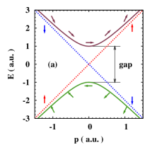
Figure 4: (Color online) (a) Spectrum $\pm E_{p}$ (full curves) and spin configuration of quasi-particle in the helical SDW state compared with the initial spectrum $\xi_{p\downarrow}$ and $\xi_{p+Q\uparrow}$ (dotted curves) and spin configuration. (b) Density of states of quasi-particle in the helical SDW state.

The quasi-particle in the helical SDW phase are described by $\eta_{p}$ and $\lambda_{p}$ with $-k_{F}<p<k_{F}$. The spectrum and density of states are plotted in Fig. 4. It is indicated that the gap opens at the Fermi surface. The spin states of quasi-particles are no longer pure spin-up or spin-down, but mixed spin state, enabling back scattering.

IV.2 Surfaces of 3D TIs with Hexagonal Fermi Surface

We first need to determine which spin density wave emerges in the SDW state. Following the Ginzburg-Landau theory, the free-energy functional can be written as

$$F_{GL}=F_{2}+F_{4h}$$ (56)

with

$$F_{2}=\frac{1}{2}\sum_{\nu,{\bf q}}\tilde{\chi}_{\nu,\nu}^{-1}({\bf q},0)|\phi_{\nu}({\bf q})|^{2}.$$ (57)

Here $\tilde{\chi}_{\nu,\nu}$ is the diagonalized and “normalized” [see Eq. (40)] spin susceptibility tensor. $\phi_{\nu}({\bf q})$ is the SDW. $F_{4h}$ denotes the free-energy to the fourth and higher orders of $\phi$. At sufficient low temperature, $\chi$ and $F_{2}$ become negative, which drives the system into the SDW state. As

$$\tilde{\chi}_{\nu,\nu}^{-1}=\frac{1-U\tilde{\chi}_{\nu\nu}^{0}}{\tilde{\chi}_{\nu\nu}^{0}}=-U+1/\tilde{\chi}_{\nu\nu}^{0},$$ (58)

the SDW with largest $\chi^{0}_{\nu\nu}$ will first emerge as temperature is lowered down. According to the discussion in Sec. III B, such spin susceptibility is $\tilde{\chi}_{G}^{0}({\bf Q}_{i},0)$ [$i=(1,2,3)$]. Therefore, the first emergent SDW is the helical SDW. As $\tilde{\chi}_{G}^{0}({\bf Q}_{i},0)$ is much larger than the others, there will be a temperature region, where only the helical SDW emerges. The following discussion is restricted in this temperature region.note2

Free energy $F_{2}$ of the concerned helical SDWs is,

$$F_{2}=\frac{1}{2}\sum_{i}\tilde{\chi}_{G}^{-1}({\bf Q}_{i},0)|\phi_{i}|^{2},$$ (59)

with

$$\phi_{i}\equiv\langle\tilde{\sigma}_{G}({\bf Q}_{i})\rangle$$ (60)

being complex. According to Eq. (43), $F_{GL}$ should be invariant under the symmetry operations:

$$\phi_{i}\to\phi_{i+1},\quad\phi_{i}\leftrightarrow-\phi_{i}^{\ast}.$$ (61)

The $C_{3v}$ symmetry also gives another invariant operation,

$$\phi_{i}\to\phi_{i-1}.$$ (62)

Besides, $F_{GL}$ respects the translational symmetry,

$${\bf r}\to{\bf r}+{\bf d}:\phi_{i}\to\phi_{i}e^{{\rm i}{\bf Q}_{i}\cdot{\bf d}}.$$ (63)

Therefore, the symmetry allowed terms in $F_{GL}$ at the fourth order are,

$$F_{4}=\sum_{i}u_{41}|\phi_{i}|^{4}+u_{42}|\phi_{i}|^{2}|\phi_{i+1}|^{2}.$$ (64)

To the sixth order,

$$F_{6} = \sum_{i}u_{61}|\phi_{i}|^{6}+u_{62}(|\phi_{i}|^{4}|\phi_{i+1}|^{2}+|\phi_{i}|^{2}|\phi_{i+1}|^{4})$$ (65)

$$\mbox{}~{}+u_{63}[(\phi_{1}\phi_{2}\phi_{3})^{2}+(\phi_{1}^{\ast}\phi_{2}^{\ast}\phi_{3}^{\ast})^{2}],$$

where the last term appears due to the translational sysmmetry and $\sum_{i}{\bf Q}_{i}=0$.Fu Those higher order terms determines whether the three SDWs coexist or only one of the SDWs is allowed (the stripe phase). Explicitly, after reorganization, there are terms like $(|\phi_{i}|^{2}-|\phi_{i+1}|^{2})^{2n}$ with $n\geq 1$, which prefer the difference $|(|\phi_{i}|^{2}-|\phi_{i+1}|^{2})|$. If those terms are prominent, the stripe phase is favored.

Below, we explore a mean field theory to describe the helical SDW states on the surfaces of 3D TIs. For simplicity, we restrict ourself to the stripe phase, where only one helical SDW exists. The mean field Hubbard Hamiltonian is

$$H_{U}=-\frac{U}{a_{G}}\sum_{i}\left[\tilde{\sigma}_{G}({\bf Q}_{i})\phi_{i}^{\ast}+(\tilde{\sigma}_{G}({\bf Q}_{i}))^{\dagger}\phi_{i}-|\phi_{i}|^{2}\right],$$ (66)

The magnitude $|\phi_{i}|$ is determined by minimizing the Ginzburg-Landau free energy, whereas phase fluctuation of $\phi_{i}$ correspond to the gapless the spin wave excitations (Goldstone modes). In the stripe phase, only one of the three $|\phi_{i}|$ is nonzero. The mean field Hamiltonian is

$$H_{\rm MF}=\frac{U}{a_{G}}\sum_{i}|\phi_{i}|^{2}+$$

$$\hskip 2.84544pt\sum_{{\bf k},i}{}^{\prime}\left(\begin{array}[]{cc}c^{\dagger}_{{\bf k}+}&c^{\dagger}_{{\bf k+Q}_{i}+}\end{array}\right)\left(\begin{array}[]{cc}\xi_{{\bf k}+}&B_{i}g_{i}({\bf k})\\ B_{i}^{\ast}g_{i}^{\ast}({\bf k})&\xi_{{\bf k+Q}_{i}+}\end{array}\right)\left(\begin{array}[]{c}c_{{\bf k}+}\\ c_{{\bf k+Q}_{i}+}\end{array}\right),$$ (72)

with

$$g_{i}({\bf k})=\langle u_{+}({\bf k})|\tilde{\sigma}_{G}({\bf Q}_{i})|u_{+}({\bf k+Q}_{i})\rangle,\quad B_{i}=-\frac{U}{a_{G}}\phi_{i}^{\ast}.$$ (74)

The summation $\sum_{\bf k}^{\prime}$ is restricted in certain region as ${\bf k}$ and ${\bf k+Q}_{i}$ dictate the same Hamiltonian. For example, for the case where only $\phi_{1}$ is nonzero, ${\bf k}$ is restricted in the region where $-Q_{1}\leq k_{x}<0$ as ${\bf Q}_{1}=(Q_{1},0)$. A significant feature of the Hamiltonian is that both the diagonal and off-diagonal terms are ${\bf k}$-dependent, which may induce nontrivial Berry curvature in some cases. But we will not discuss this important property here. The mean field Hamiltonian is diagonalized as

$$H_{\rm MF}=\sum_{{\bf k},i}{}^{\prime}\left[E_{i{\bf k}+}\eta_{i{\bf k}}^{\dagger}\eta_{i{\bf k}}+E_{i{\bf k}-}\lambda_{i{\bf k}}^{\dagger}\lambda_{i{\bf k}}\right]+\frac{U}{a_{G}}\sum_{i}|\phi_{i}|^{2},$$ (75)

via the following Bogoliubov transformation,

$$\eta_{i{\bf k}} = u_{i{\bf k}}e^{-{\rm i}\psi_{i{\bf k}}}c_{{\bf k}+}-v_{i{\bf k}}c_{{\bf k+Q}_{i}+}$$

$$\lambda_{i{\bf k}} = v_{i{\bf k}}e^{-{\rm i}\psi_{i{\bf k}}}c_{{\bf k}+}+u_{i{\bf k}}c_{{\bf k+Q}_{i}+},$$ (76)

with

$$u_{i{\bf k}} = \frac{1}{\sqrt{2}}\sqrt{1+\frac{\zeta_{i{\bf k}}}{\sqrt{\zeta_{i{\bf k}}^{2}+|B_{i}g_{i}({\bf k})|^{2}}}},$$

$$v_{i{\bf k}} = \frac{1}{\sqrt{2}}\sqrt{1-\frac{{\zeta_{i{\bf k}}}}{\sqrt{\zeta_{i{\bf k}}^{2}+|B_{i}g_{i}({\bf k})|^{2}}}}.$$ (77)

and $\psi_{i{\bf k}}={\rm Arg}[B_{i}g_{i}({\bf k})]$, ${\zeta_{i{\bf k}}}=\frac{1}{2}(\xi_{{\bf k}+}-\xi_{{\bf k+Q}_{i}+})$. The energy spectrum of the quasi-particle excitation is

$$E_{i{\bf k}\pm}=\pm\sqrt{\zeta_{i{\bf k}}^{2}+|B_{i}g_{i}({\bf k})|^{2}}+\frac{1}{2}(\xi_{{\bf k}+}+\xi_{{\bf k+Q}_{i}+}).$$ (78)

It should be mentioned that although the energy gap is ${\bf k}$-dependent, it does not close at any ${\bf k}$.

V Helical magnetic order in the magnetically doped surfaces of 3D TIs

The magnetic order in the magnetically doped surfaces of 3D TIs has attracted a lot of interest.MnDoped1 ; MnDoped2 ; Wray ; QinLiu ; aniso ; Abanin Theoretical investigationQinLiu has shown that the Ruderman-Kittel-Kasuya-Yosida (RKKY) interaction is always ferromagnetic when the Fermi energy is close to the Dirac point. When a ferromagnetic order emerges, a gap is opened around the Dirac point. Recent experiments confirmed such results in Mn or Fe doped Bi₂Se₃ and Bi₂Te₃.MnDoped1 ; MnDoped2 ; Wray

Here we consider the situation when the Fermi energy is much higher and the Fermi surface is hexagonal (and hence nested). From the discussion in previous sections, we know that the spin susceptibility function is peaked at the nesting wavevector where it is helical. Physically, the effective interaction between two magnetic impurities are mediated by the carrier spin density excited by one of the impurity and feeled by another. The spin susceptibility function describes such excitation. The nature of the spin susceptibility thus has profound implication on the effective interaction and the magnetic order.

The above picture can be described well by the mean field Zener theory, which has been shown to be successful in the theory of dilute III(Mn)-V magnetic semiconductors.rmp The Hamiltonian of the system is

$$H=H_{STI}-J\sum_{iI}{\bf S}_{I}\cdot{\bf s}_{i},$$ (79)

where $H_{STI}$ is the Hamiltonian of carriers in the surfaces of 3D TIs. The last term describes the carrier–magnetic-impurity exchange interaction. $I$ and $i$ label magnetic impurities and carriers respectively (with spin ${\bf S}_{I}$ and ${\bf s}_{i}$ respectively).

In Zener theory, the equilibrium mean carrier and magnetic-impurity spin densities are calculated by minimizing the Ginzburg-Landau free energy. Under the mean field approximation and neglect higher order correlations, the free energy functional istomas

$$F_{GL}[\phi] = -n_{M}k_{B}T\ln\left[\sum_{j=-S}^{S}\exp(J\phi j/Lk_{B}T)\right]+F_{c}[\phi]$$ (80)

$$\mbox{}~{}-J\phi SB_{S}(SJ\phi/Lk_{B}T),$$

where $\phi=\sqrt{\sum_{\mu}|\phi_{\mu}|^{2}}$ is the mean carrier spin density. $L$ is the width of surface channel. The first term in right hand side is the free energy of magnetic impurities with $S$ being the total spin quantum number of a single impurity. $n_{M}$ denotes the density of magnetic impurities. The second and third terms are the free energy of the carrier system. The last term is the energy of carrier spin density under the mean field of the exchange interaction, with $B_{S}$ being the Brillouin function.

The underlying physics is that, the increase in carrier spin density $\phi$ reduces the first and last terms in the Ginzburg-Landau free energy, whereas it costs by increasing $F_{c}[\phi]$ as the carrier system is in the paramagnetic state. The equilibrium value of $\phi$ is determined by minimizing $F_{GL}[\phi]$. At small carrier spin density (the “linear susceptibility regime”), $F_{c}[\phi]$ can be written as

$$F_{c}[\phi]=\frac{1}{2L}\sum_{\nu,{\bf q}}\tilde{\chi}_{\nu,\nu}^{-1}({\bf q})|\phi_{\nu}({\bf q})|^{2}$$ (81)

where $\tilde{\chi}_{\nu\nu}$ is the diagonalized and “normalized” [see Eq. (40)] spin susceptibility. It is noted that the spin density $\phi_{\nu}({\bf q})$ corresponding to the largest $\tilde{\chi}_{\nu\nu}({\bf q})$ is energetically favored as it minimizes $F_{c}[\phi]$. In previous sections, we have shown that the largest spin susceptibility is achieved at $\tilde{\chi}_{G}({\bf Q}_{i})$. [see Fig. 3], where the corresponding $\phi_{G}({\bf Q}_{i})$ is a helical spin density wave. Therefore, the energetically favored magnetic order is the helical magnetic order, when Fermi surface is nested.

It should be pointed out that the above equations can also be used to obtain the Curie temperature of the magnetic order tomas ; rmp

$$k_{B}T_{C}=\frac{S(S+1)}{3}\frac{J^{2}n_{M}\tilde{\chi}_{G}({\bf Q}_{i},0)}{L}.$$ (82)

The mean carrier spin density is a stripe helical one at the nesting wave-vector ${\bf Q}_{i}$. The spins of magnetic impurities are aligned parallel or anti-parallel to the carrier spin density at their local positions, depending on the sign of the exchange constant $J$. Explicitly, the mean carrier spin density is

$$\langle\sigma_{\mu}({\bf r})\rangle=\sum_{i}\langle\sigma_{\mu}({\bf Q}_{i})\rangle e^{{\rm i}{\bf Q}_{i}\cdot{\bf r}}+c.c.,$$ (83)

where

$$\langle\sigma_{\mu}({\bf Q}_{i})\rangle=\frac{{G}_{i\mu}}{\sqrt{a_{G}}}\phi_{i},$$ (84)

with ${\mu}=(x,y,z)$ and $\phi_{i}=\langle\tilde{\sigma}_{G}({\bf Q}_{i})\rangle$ is complex. Here $a_{G}$ is defined in Eq. (38) and ${G}_{i\mu}$ is defined in Eq. (42) [the special case $i=1$ is given approximately in Eq. (34)].

The amplitude $\phi=|\phi_{i}|$ is determined by minimizing $F_{GL}[\phi]$. There are three energetically favored configurations corresponding to the three ${\bf Q}_{i}$. For each configuration, the magnetic anisotropy is expected to be very large, as the spin susceptibility tensor $\hat{\chi}({\bf Q}_{i},0)$ is highly anisotropic [it has an eigen-value much larger than the other two, see Fig. 2(b)].

According to our calculation, for Mn doped Bi₂Te₃ surface states with $E_{F}\simeq 0.7E_{s}$ (0.2 eV, corresponding electron density $4\times 10^{12}$ cm^-2), $\tilde{\chi}_{G}\simeq 0.3*10^{-2}$ Å^-2eV^-1 [see Fig. 3(a)], $J\simeq 10^{2}$ eV Å³,Dai the width of surface channel $L=50$ Å  (inferred from Ref. YLChen, ), $n_{M}=2\times 10^{-3}$ Å^-3($\simeq 0.1$ mole fraction), $S=5/2$, we get $T_{C}\simeq 30$ K, which is not very low.

It should be pointed out that further investigations on the problem are demanded. On one hand, the carrier–magnetic-impurity exchange interaction, which leads to carrier spin relaxation and shortens the propagating distance of the carrier SDW excited by magnetic impurities, should be included in the calculation of the spin susceptibility function. On the other hand, the exchange and correlation corrections to the spin susceptibility function should be included.rmp A density-functional calculation will be appreciated.rmp Via such improvement, the magnetization can be calculated at arbitrary temperature, carrier and magnetic-impurity densities. We believe that the helical magnetic order is still favored after those corrections are included, according to the symmetry of the system. We assumed that the electron density can be tuned either by gate-voltage or doping by other dopants besides ferromagnetic impurities, which is in principle achievable in experiments.rmp

Finally, we note that very recently, Ye et al. found that the helical magnetic order emerges in a chain of impurity spins in the surfaces of 3D TIs.spin-helix And Zhu et al. discussed the RKKY interaction when Fermi surface is hexagonal.Zhu

VI Conclusion

We study spin susceptibility and magnetic order at the edges/surfaces of topological insulators when the Fermi surface is nested. We find that due to spin-momentum locking as well as time-reversal symmetry, spin susceptibility at the nesting wavevector has a strong helical feature. It follows then, a helical SDW state emerges at low temperature due to Fermi surface nesting. The helical feature of spin susceptibility also has profound impact on the magnetic order in the magnetically doped surfaces of 3D TIs. From the Zener theory, to the lowest order, we predicted a helical magnetic order in such system.

The helical SDW order can be probed/determined either directly by spin resolved STM or indirectly by the existence of an energy gap at the Fermi surface via, e.g., ARPES. For spin pump-probe measurements, if a local spin density is excited, it will propagator with certain helicity along the nesting wavevectors. The helical magnetic order in magnetically doped surface of 3D TIs can also be probed directly by spin resolved STM and other magnetic response measurements.

Finally, recent studies indicate that topological insulators can also be achieved in cold-atom systems.cold-atom The tunability of inter-particle interaction (and many other properties) in such systems may be utilized to enhance the helical SDW order predicted in this paper.

References

• (1) C. L. Kane and E. J. Mele, Phys. Rev. Lett. 95, 146802 (2005).
• (2) B. A. Bernevig, T. A. Hughes, and S.-C. Zhang, Science 314, 1757 (2006).
• (3) L. Fu, C. L. Kane, and E. J. Mele, Phys. Rev. Lett. 98, 106803 (2007).
• (4) L. Fu and C. L. Kane, Phys. Rev. B 76, 045302 (2007).
• (5) J. E. Moore and L. Balents, Phys. Rev. B 75, 121306(R) (2007).
• (6) R. Roy, Phys. Rev. B 79, 195322 (2009).
• (7) M. König, S. Wiedmann, C. Brüne, A. Roth, H. Buhmann, L. W. Molenkamp, X. L. Qi, and S.-C. Zhang, Science 318, 766 (2007).
• (8) D. Hsieh, D. Qian, L. Wray, Y. Xia, Y. S. Hor, R. J. Cava, and M. Z. Hasan, Nature (London) 452, 970 (2008).
• (9) Y. Xia, D. Qian, D. Hsieh, L. Wray, A. Pal, H. Lin, A. Bansil, D. Grauer, Y. S. Hor, R. J. Cava, and M. Z. Hasan, Nat. Phys. 5, 398 (2009).
• (10) Y. L. Chen, J. G. Analytis, J.-H. Chu, Z. K. Liu, S.-K. Mo, X. L. Qi, H. J. Zhang, D. H. Lu, X. Dai, Z. Fang, S.-C. Zhang, I. R. Fisher, Z. Hussain, and Z.-X. Shen, Science 325, 178 (2009).
• (11) C. Wu, B. A. Bernevig, and S.-C. Zhang, Phys. Rev. Lett. 96, 106401 (2006).
• (12) H. Zhang, C. X. Liu, X. L. Qi, X. Dai, Z. Fang, and S.C. Zhang, Nat. Phys. 5, 438 (2009).
• (13) D. Hsieh, Y. Xia, D. Qian, L. Wray, J. H. Dil, F. Meier, J. Osterwalder, L. Patthey, J. G. Checkelsky, N. P. Ong, A. V. Fedorov, H. Lin, A. Bansil, D. Grauer, Y. S. Hor, R. J. Cava, and M. Z. Hasan, Nature 460, 1101 (2009).
• (14) Y. Okada, C. Dhital, W.-W. Zhou, H. Lin, S. Basak, A. Bansil, Y.-B. Huang, H. Ding, Z. Wang, S. D. Wilson, and V. Madhavan, arXiv:1011.4913
• (15) D. Hsieh, Y. Xia, D. Qian, L. Wray, F. Meier, J. H. Dil, J. Osterwalder, L. Patthey, A. V. Fedorov, H. Lin, A. Bansil, D. Grauer, Y. S. Hor, R. J. Cava, and M. Z. Hasan, Phys. Rev. Lett. 103, 146401 (2009)
• (16) K. Kuroda, M. Arita, K. Miyamoto, M. Ye, J. Jiang, A. Kimura, E. E. Krasovskii, E. V. Chulkov, H. Iwasawa, T. Okuda, K. Shimada, Y. Ueda, H. Namatame, and M. Taniguchi, Phys. Rev. Lett. 105, 076802 (2010).
• (17) K. Kuroda, M. Ye, A. Kimura, S. V. Eremeev, E. E. Krasovskii, E. V. Chulkov, Y. Ueda, K. Miyamoto, T. Okuda, K. Shimada, H. Namatame, and M. Taniguchi, Phys. Rev. Lett. 105, 146801 (2010).
• (18) S.-Y. Xu, L.A. Wray, Y. Xia, R. Shankar, S. Jia, A. Fedorov, J. H. Dil, F. Meier, B. Slomski, J. Osterwalder, R. J. Cava, M. Z. Hasan, arXiv:1008.3557
• (19) Y. L. Chen, Z. K. Liu, J. G. Analytis, J.-H. Chu, H. J. Zhang, S.-K. Mo, R. G. Moore, D. H. Lu, I. Fisher, S. C. Zhang, Z. Hussain, Z.-X. Shen, arXiv:1006.3843
• (20) S.-Y. Xu, L. A. Wray, Y. Xia, R. Shankar, A. Petersen, A. Fedorov, H. Lin, A. Bansil, Y. S. Hor, D. Grauer, R. J. Cava, and M. Z. Hasan, arXiv:1007.5111
• (21) M. Z. Hasan and C. L. Kane, Rev. Mod. Phys. 82, 3045 (2010).
• (22) R. Yu, W. Zhang, H.-J. Zhang, S.-C. Zhang, X. Dai, and Z. Fang, Science 329, 61 (2010).
• (23) A. Agarwal, S. Chesi, T. Jungwirth, J. Sinova, G. Vignale, and M. Polini, arXiv:1010.5169
• (24) X.-L. Qi and S.-C. Zhang, arXiv:1008.2026
• (25) D. D. Awschalom, D. Loss, and N. Samarth, Semiconductor Spintronics and Quantum Computation (Springer, Berlin, 2002); I. Žutić, J. Fabian, and S. D. Sarma, Rev. Mod. Phys. 76, 323 (2004); J. Fabian, A. Matos-Abiague, C. Ertler, P. Stano, and I. Žutić, Acta Phys. Slovaca 57, 565 (2007); M. I. D’yakonov, Spin Physics in Semiconductors (Springer, Berlin, 2008); M. W. Wu, J. H. Jiang, and M. Q. Weng, Phys. Rep. 493, 61 (2010).
• (26) Z. Alpichshev, J. G. Analytis, J.-H. Chu, I. R. Fisher, Y. L. Chen, Z. X. Shen, A. Fang, and A. Kapitulnik, Phys. Rev. Lett. 104, 016401 (2010).
• (27) L. Fu, Phys. Rev. Lett. 103, 266801 (2009).
• (28) C.-X. Liu, X.-L. Qi, H.-J. Zhang, X. Dai, Z. Fang, and S.-C. Zhang, Phys. Rev. B 82, 045122 (2010).
• (29) If exchange and correlation effects are taken into account, Coulomb interaction can also affect spin susceptibility, which is beyond the scope of this paper.
• (30) T. Giamarchi, Quantum Physics in One Dimension (Oxford University Press, Oxford, 2004).
• (31) M. Kharitonov, arXiv:1004.0194.
• (32) As $\tilde{\chi}_{G}^{0}({\bf Q}_{i},0)\propto k_{s}^{2}/E_{s}$, the critical temperature of the phase transition increases with Hubbard $U$ and $k_{s}^{2}/E_{s}$. However, to our knowledge, there is no information on $U$ in the concerned materials. We are thus unable to estimate the critical temperature.
• (33) Y. L. Chen, J.-H. Chu, J. G. Analytis, Z. K. Liu, K. Igarashi, H.-H. Kuo, X. L. Qi, S. K. Mo, R. G. Moore, D. H. Lu, M. Hashimoto, T. Sasagawa, S. C. Zhang, I. R. Fisher, Z. Hussain, Z. X. Shen, Science 329, 659 (2010).
• (34) Y. S. Hor, P. Roushan, H. Beidenkopf, J. Seo, D. Qu, J. G. Checkelsky, L. A. Wray, D. Hsieh, Y. Xia, S.-Y. Xu, D. Qian, M. Z. Hasan, N. P. Ong, A. Yazdani, and R. J. Cava, Phys. Rev. B 81, 195203 (2010).
• (35) L. A. Wray, Y. Xia, S.-Y. Xu, R. Shankar, Y. S. Hor, R. J. Cava, A. Bansil, H. Lin, and M.Z. Hasan, arXiv:1009.6216
• (36) Q. Liu, C.-X. Liu, C. Xu, X.-L. Qi, and S.-C. Zhang, Phys. Rev. Lett. 102, 156603 (2009).
• (37) A. S. Núñez and J. Fernández-Rossier, arXiv:1003.5931
• (38) D. A. Abanin and D. A. Pesin, Phys. Rev. Lett. 106, 136802 (2011).
• (39) T. Jungwirth, J. Sinova, J. Mašek, J. Kučera, and A. H. MacDonald, Rev. Mod. Phys. 78, 809 (2006).
• (40) T. Jungwirth, W. A. Atkinson, B. H. Lee, and A. H. MacDonald, Phys. Rev. B 59, 9818 (1999).
• (41) F. Ye, G. H. Ding, H. Zhai, and Z. B. Su, Europhys. Lett. 90, 47001 (2010).
• (42) J.-J. Zhu, D.-X. Yao, S.-C. Zhang, and K. Chang, Phys. Rev. Lett. 106, 097201 (2011).
• (43) e.g., T. D. Stanescu, V. Galitski, and S. Das Sarma, Phys. Rev. A 82, 013608 (2010); N. Goldman, I. Satija, P. Nikolic, A. Bermudez, M. A. Martin-Delgado, M. Lewenstein, I. B. Spielman, Phys. Rev. Lett. 105, 255302 (2010).