A statistical mechanics approach to Granovetter theory

————————————————————————————————————

Abstract.

In this paper we try to bridge breakthroughs in quantitative sociology/econometrics pioneered during the last decades by Mac Fadden, Brock-Durlauf, Granovetter and Watts-Strogats through introducing a minimal model able to reproduce essentially all the features of social behavior highlighted by these authors.
Our model relies on a pairwise Hamiltonian for decision maker interactions which naturally extends the multi-populations approaches by shifting and biasing the pattern definitions of an Hopfield model of neural networks. Once introduced, the model is investigated trough graph theory (to recover Granovetter and Watts-Strogats results) and statistical mechanics (to recover Mac-Fadden and Brock-Durlauf results). Due to internal symmetries of our model, the latter is obtained as the relaxation of a proper Markov process, allowing even to study its out of equilibrium properties.
The method used to solve its equilibrium is an adaptation of the Hamilton-Jacobi technique recently introduced by Guerra in the spin glass scenario and the picture obtained is the following: just by assuming that the larger the amount of similarities among decision makers, the stronger their relative influence, this is enough to explain both the different role of strong and weak ties in the social network as well as its small world properties. As a result, imitative interaction strengths seem essentially a robust request (enough to break the gauge symmetry in the couplings), furthermore, this naturally leads to a discrete choice modelization when dealing with the external influences and to imitative behavior a la Curie-Weiss as the one introduced by Brock and Durlauf.

1 Summarizing some main results of quantitative sociology

In recent years there has been an increasing awareness towards the problem of finding a quantitative way to study the role played by human interactions in shaping behavior observed at a population level, ranging from the context of pure sociology to the one belonging to economic sciences. The conclusion reached by all these studies is that mathematical models have the potential of describing several features of social behavior, among which, for example, the sudden shifts often observed in society’s aggregate behavior [30][35][29], and that these are unavoidably linked to the way individual people influence each other when deciding how to behave (the phase transitions in the language of thermodynamics [18]), the whole suggesting a promising potential application of disordered statistical mechanics to this field of research [2][13][17].
Here we summarize what we understood as real breakthroughs in these analysis, highlighting two main aspects dealing with topological investigations on the structure of the graph built by social interactions and the kind of interactions themselves. Namely, the discovery of the fundamental role of weak ties in bridging different communities (due to Granovetter [13, 24, 25, 26]) and the “small world” feature of the social structure (obtained by Watts and Strogatz [15, 38, 39]) for the first analysis and the discrete choice of decision makers in econometric (due to Mac Fadden [19, 34, 28]) and the essentially imitative behavior among these agents (due to Brock and Durlauf [12, 17, 18]).

Even though fundamental experiments dealing with social networks may constellate modern society analysis (i.e. the paradigmatic Milgram experiment of the sixties [33]), a real breakthrough in our understanding of network structure inside modern societies has been achieved when Granovetter reversed the Chicago school of social-psychology showing how a person with built weak ties (which were previously seen, at individual level, as ancestors of depressive states) was much more able to adapt its behavior to the social fitness due to the much broader amount of available information: in particular he noticed that these weak ties may often carry information of little significance (but not redundant as in highly clusterized community of similar agents linked by strong ties), however they allow a primarily transmission of new information across otherwise disconnected cluster of the social network (allowing great potential benefit by these bridges).
Two decades after this achievement, Watts and Strogatz, trough a mathematical technique (rewiring) have been able to display the Milgram results (sometimes known as “six degrees of separation”) by which they understood that social (as well as others, i.e. biological [1][5]) networks can not be described by purely ordered or purely random graphs (i.e. Erdos-Renyi ones [5, 36]) due to correlations among nodes which allow for a much faster transmission of information (real graphs show high degree of cliqueness [37, 10]), pioneering a quantitative approach to these new networks, nowadays often called ”small worlds”.

In a different but related context, Mac Fadden has shown how to infer a model for econometric estimation of binary decision making (reflecting accurately several real cases in social structures [31]) by introducing fundamental dichotomic degrees of freedom inside each agent mirroring its personal attitudes (i.e. a bit string $\mathbb{\xi}$ of $K$ entries $\mu=1,...,K$ where each entry represent an attribute, i.e. $\mu=1$ accounting for smoking such that $\xi_{i}^{\mu=1}=+1$ states that the i agent smokes while $\xi_{i}^{\mu=1}=0$ states that he does not, and so on). Once indexed individuals by $i,\ i=1...N$, and assigned an Ising spin to each individual’s choice $\sigma_{i}=+1$ for the agreement or $\sigma_{i}=-1$ for disagreement, he chooses to exploit data by assuming a single particle model into a suitable external field $h_{i}$ (the “field” influencing the choice of $i$) which is a function of the vector of attributes $\xi_{i}$. Since for the sake of simplicity attributes are taken as binary variables, the whole theory can be described in terms of an effective one-body Hamiltonan $H$ as

$$H_{N}(\sigma;\xi)=\sum_{i}^{N}h_{i}\sigma_{i}=\frac{h}{K}\sum_{i}^{N}\sum_{\mu}^{K}\xi_{h}^{\mu}\xi_{i}^{\mu}\sigma_{i},$$

where $h$ is a scalar parameter ruling the overall intensity of the external stimulus (whose capabilities of influencing a generic agent $i$ are encoded into its bit-string $\xi_{h}$). This parametrization of $h_{i}$ correspond to what economists call a discrete choice model [34], and shows a remarkable link between econometrics and statistical mechanics ($H_{N}(\sigma;\xi)$ can be seen as a random field Ising model): In fact discrete choice theory has the same variational flavour of thermodynamics as states that, when making a choice, each person weights out various factors such as his own gender, age, income, etc, as to maximize in probability the benefit arising from his/her decision.

Despite this result, there exist many examples from economics and sociology where it has been observed how the global behavior of large groups of people can change in an abrupt manner as a consequence of slight variations in the social structure (such as, for instance, a change in the pronunciation of a language due to a little immigration rate, or as a substantial decrease in crime rates due to seemingly minor action taken by the authorities [29, 11]). From a statistical mechanical point of view, these abrupt transitions should be considered as phase transitions caused by the interaction between individuals that can not be accounted by a pure one-body theory. Indeed, Brock and Durlauf have shown [12] how discrete choice can be extended to the case where a global mean-field interaction is present (providing an interesting mapping to the Curie-Weiss theory (CW) [18, 6]), thus further highlighting the close relation existing between the econometric and the statistical mechanical approaches to these problems.

Instead of introducing Brock-Durlauf approach (which is a systematic translation of the CW scenario in social sciences) we go one step forward following the subsequent generalization obtained by diving the ensemble of the N decision makers into clusters, due to Contucci and coworkers [19, 20]: Introducing a general two-body Hamiltonian $H_{N}(\sigma;J)$ as

$$H_{N}(\sigma;J)=-\sum_{i,l=1}^{N}J_{il}\sigma_{i}\sigma_{l}-\sum_{i=1}^{N}h_{i}\sigma_{i},$$ (1.1)

they went over by defining a suitable parametrization for the interaction coefficients $J_{il}$. Since each agent is characterized by $k$ binary socio-economic attributes, the population can be naturally partitioned into $2^{k}$ subgroups, which for convenience are taken of equal size: this leads to consider a mean field kind of interaction, where coefficients $J_{il}$ depend explicitly on such a partition as follows

$$J_{il}=\frac{J}{2^{k}\,N}\delta_{gg^{\prime}},\ \textrm{if $i\in g$ and $l\in g^{\prime}$},$$

which in turn allows us to rewrite (1.1) as

$$H_{N}(\sigma;J)=-\frac{NJ}{2^{k}}(\sum_{g,g^{\prime}=1}^{2^{k}}\delta_{gg^{\prime}}m_{g}m_{g^{\prime}}+\sum_{g=1}^{2^{k}}h_{g}m_{g})$$

where $m_{g}$ is the average opinion of group $g$, namely $m_{g}=\frac{1}{2^{k}\,N}\sum_{i=(g-1)N/2^{k}+1}^{g\,N/2^{k}}\sigma_{i}$.
This idea of partitioning the interaction matrix into clusters of similar agents can be extended to a natural limit (that we work out here) such that the size of these clusters approaches zero in the thermodynamic limit (so to preserve each individual identity and uniqueness for each agent, or a measure of attitude fluctuations inside the original idea of clusters): interestingly this leads to an interaction matrix so that

$$J_{ij}=\frac{1}{K}\sum_{\mu}^{K}\xi_{i}^{\mu}\xi_{j}^{\mu},$$ (1.2)

and naturally collapses the concept of magnetization in spin glasses [32] to the one of retrieval in neural networks [4], ultimately switching frustration into dilution (as $\xi\in[0,+1]$ instead of $\xi\in[-1,+1]$).

2 The model and its topology: graph theory

In this section we look at the population as a graph and we study its topological properties: each agent $i$ is represented by a node; couples of agents $(i,j)$ displaying a positive coupling $J_{ij}>0$ are said to be in contact or to interact with each other and this is envisaged by means of a link between $i$ and $j$, whose weight is just $J_{ij}$ (cft. eq.1.2). This picture mirrors the idea that socio-economic relations between individuals or firms are embedded and organized in actual social networks, which follows from the seminal work by Granovetter.

As anticipated, each agent $i$ is characterized by a binary string $\xi_{i}$, which might be thought of as the codification of agent’s attitude, either positive ($1$) or negative ($0$), towards a given issue. All strings are taken of length $K$ and each entry is extracted randomly according to

$$P(\xi_{i}^{\mu}=+1)=\frac{1+a}{2},\;\;P(\xi_{i}^{\mu}=0)=\frac{1-a}{2},$$ (2.1)

in such a way that, by tuning the parameter $a\in[-1,+1]$, the concentration of non null-entries for the $i$-th string $\rho_{i}=\sum_{\mu}\xi_{i}^{\mu}$ can be varied; consistently, also the topology generated by the rule in Eq. 1.2 is varied. In particular, when $a\to-1$ the system is completely disconnected (and only discrete choice survives), while when $a\to+1$ each link is present, being $J_{ij}=1$ for any couple (so to retain the fully Brock-Durlauf approach). As we will see, small values of $a$ give rise to highly correlated, diluted networks, while, as $a$ gets larger the network gets more and more connected and correlation among links vanishes. In agreement with our modelization intent, repetitions among strings are allowed.

The main topological features of the emergent network have been investigated in [1, 7], where it was shown that the average link probability among two generic nodes is

$$p=1-\left[1-\left(\frac{1+a}{2}\right)^{2}\right]^{K},$$ (2.2)

and that, for large enough $N$ and $K$, with $K$ growing slower than linearly with $N$, the degree distribution is multimodal. Therefore, the average degree for a generic node reads as $z=pN$.
Apart from these global, long-scale features, the model also displays interesting properties concerning correlation among links, as we are going to deepen.

Small-world (SW) networks are characterized by two basic properties, that are a large clustering coefficient, i.e. they display subnetworks where almost any two nodes within them are connected, and a small diameter, i.e. the mean-shortest path length among two nodes grows logarithmical with $N$. While the latter requirement is a common property of random graphs [36, 5], and is therefore satisfied also by the graph under study, the clustering coefficient deserves more attention. Several attempts in the past have been made in order to define network models able to display such a feature [36, 5, 38]. For instance, in their seminal work, Watts and Strogatz [38] introduced a rewiring procedure on links, which can yield the desired degree of correlation. As we are going to show, in our approach SW effects emerge naturally from the definition of patterns and from the rule in Eq. 1.2, that is to say, interactions based on sharing of interests (i.e. non-null entries) intrinsically generate a clustered society.

Before proceeding, we notice that the same property can be addressed in different ways: we can say that the graph exhibits a large transitivity, meaning that if $i$ is connected to both $j$ and $k$, then $j$ and $k$ are likely to be connected; in modern network theory we say that the graph displays a large “cliquishness” and we measure it by means of the so-called clustering coefficient [36, 10]: The local clustering coefficient for node $i$ is defined as

$$c_{i}=\frac{2E_{i}}{z_{i}(z_{i}-1)},$$ (2.3)

where $E_{i}$ is the number of actual links present within the neighborhood of $i$, whose upper bound is just $z_{i}(z_{i}-1)/2$, namely is the number of connections for a fully connected group of $z_{i}$ neighbors nodes. Then, the (global) clustering coefficient for the whole graph simply follows as the average of $c_{i}$ over all nodes. Usually, for a graph with average degree equal to $z$, having a large clustering means that $c$ is larger than $z/N=p$, which represents the clustering coefficient $c^{\mathrm{ER}}$ for an ER random graph with an analogous degree of dilution.
As for the graph under study, we found that [7] $c\approx p+1/\rho-1/(z-1)>p$, where in the last equality we used $\rho<z-1$, which holds when $N$ is large enough and the graph topology non-trivial [7]. More generally, one can notice that for this graph, the $z_{i}$ neighbors of $i$ are all nodes displaying at least one non-null entry corresponding to any non-null entries of $\xi_{i}$; this condition biases the distribution of strings relevant to neighboring nodes, so that they are more likely to be connected with each other. Indeed, when $\rho_{i}=1$, it is easy to see that $c_{i}$=1, to be compared with $c^{\mathrm{ER}}_{i}$, namely the average link probability for node $i$, which turns out to be $(1+a)/2\leq 1$; analogous arguments apply also for larger values of $\rho$ [7]. A numerical corroboration can be found in Fig. 2.1, which shows that $c>c^{\mathrm{ER}}$ in a wide region of values of $a$ corresponding to non-trivial networks, i.e. for $a$ larger than the percolation threshold and smaller than the fully-connected threshold. The clustering effect is especially manifest in the region of high dilution, where, for graphs analyzed here, $c$ is even two orders of magnitude larger than $c^{\mathrm{ER}}$. Of course, when $a$ approaches $1$, the graph gets fully connected and $c\to c^{ER}\to 1$. These results are robust as $N$ is varied.

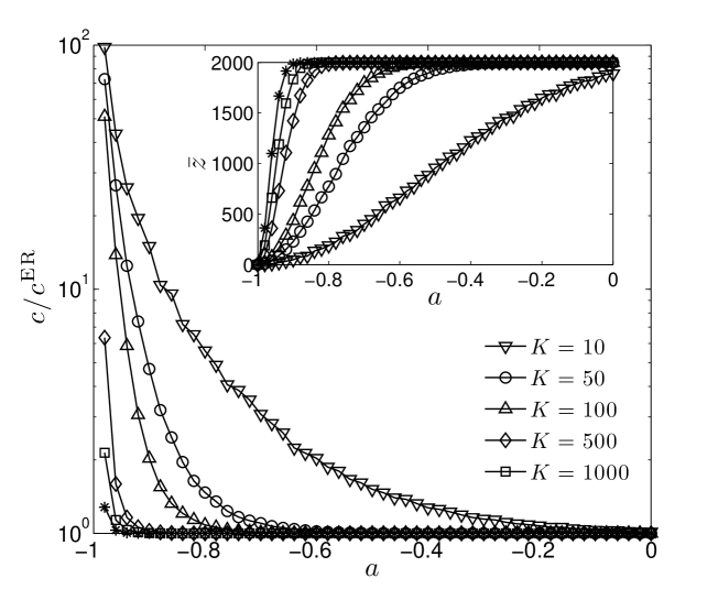
Figure 2.1: Main figure: Ratio between the clustering coefficient $c$ measured for the correlated network under consideration and the coefficient $c^{\mathrm{ER}}$ corresponding to a purely random graph displaying an analogous density of links, as a function of the parameter $a$ and for different values of $K$; the volume $N$ is kept fixed and equal to $2000$. Inset: behavior of the average degree $\bar{z}$ with respect to $a$ for the same set of realizations corresponding to the main figure.

Finally, we mention another quantity used in ecology and epidemiology to quantify the existence of correlations among links, that is the so-called assortativity coefficient [36, 37]: a network is said to show “assortative mixing” (“dissortative mixing”) on their degrees whenever high-degree vertices prefer to attach to other high-degree (low-degree) vertices. While assortativity is typical of social networks, dissortativity is often found in technological and biological networks.
The assortativity coefficient $r$ can be defined as a Pearson coefficient to measure the correlation between the coordination numbers at either ends of a link; the ER graph corresponds to $r=0$ [36]. The measures performed on the graph under study suggest a dissortative behavior ($r<0$), which is corroborated by the quantity $\langle z\rangle_{z^{\prime}}$, representing the average degree over the nearest-neighbors of a node with degree $z^{\prime}$, namely:

$$\bar{z}_{z^{\prime}}=\sum_{z=0}^{N-1}zP(z;z^{\prime}),$$ (2.4)

where $P(z;z^{\prime})$ is the conditional probability that a link stemming from a node with degree $z^{\prime}$ points to a node with degree $z$. As shown in Fig.2.2, a decreasing behavior of $\bar{z}_{z^{\prime}}$ is consistent with a dissortative mixing.

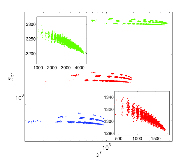
Figure 2.2: Neighbor assortativity for different system sizes (from top to bottom $N=2000,N=5000,N=8000$, depicted in different colors) and different values of $K/N$ (for each choice of $N$, from top to bottom, $K/N=25,K/N=100,K/N=250$). Notice that for $K$ small different modes can be distinguished. The two insets show in detail the case $N=2000,K=80$ (upper panel) and $N=8000,K=320$ (lower panel). The value of $a$ is fixed and equal to $-0.6$.

The reason of this behavior is clear to see: while nodes corresponding to strings with large $\rho$ can connect to most other nodes, nodes with small $\rho$ have basically no chance to connect to other similar strings. This gets more evident for $a$ small, as the concentration of such strings is larger. Interestingly, as highlighted in [37], dissortativity has significant effects on the resilience (see next section) of the structure itself: dissortatively mixed networks are less robust to the deletion of their vertices than assortatively mixed or neutral networks.

As first remarked in [24], real social networks are not only characterized by a small-world topology, which basically means large clustering and small diameter, but they also feature a peculiar coupling pattern. In fact, not only the neighbors of a given node $i$ are likely to be connected, but they form communities such that intra-group links are expected to be stronger than inter-group links. In this way weaker ties work as bridges connecting communities strongly linked up. Interestingly, analogous properties are found also for $\mathcal{G}(N,K,a)$, in fact, it is intuitive to see that nodes displaying very similar strings are likely to be intensively connected with each other, hence forming a group, while, each of them, separately and according to the pertaining string, can be weakly connected with other nodes/groups.
In order to deepen the role of weak ties, we perform two percolation processes where links are deleted either deterministically or randomly: Given the pattern of couplings, in the former case we delete those with magnitude lower than a given threshold $\iota\in[0,1]$ meant as a tunable parameter; in the latter case we progressively delete nodes in a random way. We call $1-f$ the fraction of links erased (in the former case $f$ is a function of $\iota$) and we measure the size of the largest connected cluster (see also [3] for more details). Results are shown and compared in Fig. 2.3.

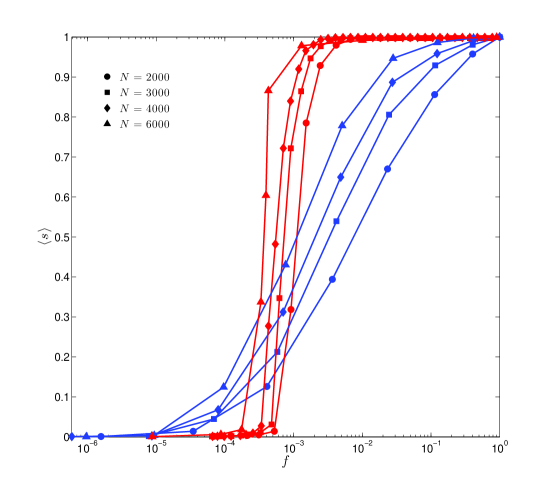
Figure 2.3: Size of the largest component versus the fraction of links in the system. Several size are depicted $N=2000$, $N=3000$, $N=4000$, $N=6000$, all corresponding to the same value $\alpha=100$ and $\gamma=1$. Notice that when weak ties are deleted first, the way the size of the largest component $\langle s\rangle$ increases with $f$ is smoother with respect to the random delation and also that $\langle s\rangle$ is smaller than $1$ at relatively large values of $f$.

Interestingly , when weak links are deleted first the graph starts to be disconnected at a value of $f$ rather small, and this is a signature that such links work as bridge. On the other hand, strong ties are highly redundant [3]. Indeed, starting from a connected graph, the first nodes to get disconnected are those with small $\rho$, to fix ideas, those with $\rho=1$; among these, the ones with the non-null entry in the same position were completely clustered in the original network. As the threshold $\iota$ is increased, more and more nodes get disconnected; most of them remain isolated (typically those with $\rho<\iota$), however, some non-trivial components survive. Such clusters are made up of very similar strings with a relatively large number of non-null entries ($\rho>\iota$) and are therefore all closely connected.

It is worth noting that such strongly clustered components emerge just in the “critical region”, namely where it is possible to detect nodes bridging two clusters and which play as “brokerage” between distinct group; this is a strategic position since it allows access to a more diverse set of ideas and information. The notions of homogeneity within groups and intermediacy between groups form the basis for the theory of ”structural holes” introduced by Burt [14].

We finally comment on the resilience properties of the network under study, which can be as well inferred from the analysis on percolation processes. According to the situation, the stability of the network can be defined as its ability to remain connected or to still exhibit a giant component, under edge removal. In the former case, if weak links are the most prone to failure, our correlated network performs rather badly. Conversely, if we are interested in the maintenance of a macroscopic connected component, given that weak links are the first to be deleted, our correlated network performs definitely better, as the percolation threshold grows slowly with $N$ (see also [3]).

3 The model and its relaxation: stochastic dynamics

We saw that the general structure of the Hamiltonian obeys

$$H_{N}(\sigma;\xi)=\frac{1}{NK}\sum_{i<j}^{N,N}\sum_{\mu=1}^{K}\xi_{i}^{\mu}\xi_{j}^{\mu}\sigma_{i}\sigma_{j}+\sum_{i}^{N}h_{i}\sigma_{i}.$$ (3.1)

It is worth recalling that the attributes ($\xi$) are drawn randomly once for all, and so ar treated as quenched variables: this does not mean that a particular agent does not evolve in time changing his attribute distribution, but that, overall, one agent may switch to another and viceversa as far as the global attribute distribution is kept constant.
The state of the system at this time is given by the average of all its building agents (such that we can introduce a ”magnetization” as their average $m=N^{-1}\sum_{i}^{N}\sigma_{i}$), each of which evolving time-step by time-step via a suitable dynamics:
Following standard disordered statistical mechanics approach [16] we introduce the latter accordingly to

$$\sigma_{i}(t+1)=sign\left(\tanh(\beta\varphi_{i}(t))+\eta_{i}(t)\right),$$ (3.2)

where $\varphi_{i}(t)$ is the overall stimulus felt by the $i$-th agent, given by

$$\varphi_{i}(t)=N^{-1}\sum_{j}^{N}J_{ij}\sigma_{j}(t)+h_{i}(t),$$ (3.3)

and the randomness is in the noise implemented via the random numbers $\eta_{i}$, uniformly drawn over the set $[-1,+1]$. $\beta$ rules the impact of this noise on the state $\sigma_{i}(t+1)$, such that for $\beta=\infty$ the process is completely deterministic while for $\beta=0$ completely random.
In the sequential dynamics we are introducing, at each time step $t$, a single agent $l_{t}$ -randomly chosen among the $N$- is updated, such that its evolution becomes

$$P[\sigma_{l_{t}}(t+1)]=\frac{1}{2}\big{(}1+\sigma_{l_{t}}(t)\tanh(\beta\varphi_{l_{t}}(t))\big{)},$$ (3.4)

whose deterministic zero-noise limit is immediately recoverable by sending $\beta\to\infty$.
If we now look at the probability of the state at a given time $t+1$, $P_{t+1}(\sigma)$, we get

$$P_{t+1}(\sigma)=\frac{1}{N}\sum_{i}^{N}\frac{1}{2}(1+\sigma_{i}\tanh(\beta\varphi_{i}(\sigma)))P_{t}(\sigma)+\frac{1}{N}\sum_{i}^{N}\frac{1}{2}(1+\sigma_{i}\tanh(\beta\varphi_{i}(F_{i}\sigma)))P_{t}(F_{i}\sigma),$$ (3.5)

where we introduced the $N$ flip-operators $F_{i}$, $i\in(1,...,N)$, acting on a generic observable $\phi(\sigma)$, as

$$F_{i}\Phi(\sigma_{1},...,+\sigma_{i},...,\sigma_{N})\ =\Phi(\sigma_{1},...,-\sigma_{i},...,\sigma_{N})$$ (3.6)

such that we can write the evolution of the network as a Markov process

$$p_{t+1}(m) = \sum_{m^{\prime}}W[m;m^{\prime}]p_{t}(m^{\prime}),$$ (3.7)

$$W[m;m^{\prime}] = \delta_{m,m^{\prime}}+\frac{1}{N}\sum_{i=1}^{N}\Big{(}w_{i}(F_{i}m)\delta_{m,Fm^{\prime}}-w_{i}(m)\delta_{m,m^{\prime}}\Big{)},$$

with the transition rates $w_{i}(m)=\frac{1}{2}[1-\sigma_{i}\tanh(\beta\varphi_{i})]$.

As the affinity matrix is symmetric, detailed balance ensures that there exists a stationary solution $P_{\infty}(m)$ such that (restricting $\tilde{h}_{i}(t)\to\tilde{h}_{i}\in\mathbb{R}\ \forall i\in(1,...,N)$)

$$W[m,m^{\prime}]P_{\infty}(m^{\prime})=W[m^{\prime},m]P_{\infty}(m).$$

This key feature ensures equilibrium, which implies

$$p_{\infty}(\sigma;J,h)\propto\exp\Big{(}\frac{\beta}{2NK}\sum_{ij}^{N}\sum_{\mu}^{K}\xi_{i}^{\mu}\xi_{j}^{\mu}\sigma_{i}\sigma_{j}-\beta\sum_{i}^{N}h_{i}\sigma_{i}\Big{)}=\exp\Big{(}-\beta H_{N}(\sigma;\xi)\Big{)},$$ (3.8)

namely the Maxwell-Boltzmann distribution [18, 6] for the Hamiltonian (3.1).
In absence of external stimuli, and skipping here the question about the needed timescales for ”thermalization”, the system reaches an equilibrium that it is possible to work out explicitly and that reproduces all the features stressed in the first section (as we are going to show).
For this detailed balanced system furthermore, the sequential stochastic process (3.2) reduces to Glauber dynamics such that the following simple expression for the transition rates $W_{i}$ can be implemented

$$W_{i}(m)=\Big{(}1+\exp(\beta\Delta H(\sigma_{i};\xi))\Big{)}^{-1},\ \ \Delta H(\sigma_{i};\xi)=H(F_{i}m;\xi)-H(m;\xi).$$ (3.9)

4 The model and its equilibrium: statistical mechanics

In the previous section we showed that, if the affinity matrix is symmetric (i.e. $J_{ij}=J_{ji}$), so that detailed balance holds, the stochastic evolution of our social model approaches the Maxwell-Boltzmann distribution (see eq.(3.8)), which determines the thermodynamic equilibria.

The latter are obtained by extremizing the free energy $A(\beta,a,h)=-\beta f(\beta,a,h)=u(\beta,a,h)-\beta^{-1}s(\beta,a,h)$ ($u$ being the internal energy and $s$ being the intensive entropy) that, as it is straightforward to check, corresponds to both maximizing entropy and minimizing energy (at the given level of noise $\beta$, attribute’s bias $a$ and external influences $h$). Furthermore, and this is the key bridge with stochastic processes, there is a deep relation among statistical mechanics and their equilibrium measure $P_{\infty}$, in fact

$$P_{\infty}(\sigma;\xi,h)\propto\exp(-\beta H(\sigma;\xi,h)),\ \ A(\beta,a,h)=-\beta f(\beta,a,h)\equiv\frac{-1}{N}\mathbb{E}\log\sum_{\sigma}\exp(-\beta H_{N}(\sigma;\xi,h)).$$

The operator $\mathbb{E}$ that averages over the quenched distribution of attributes $\xi$ makes the theory not ”sample-dependent”: For sure each realization of the network will be different with respect to some other in its details, but we expect that, after sufficient long sampling, the averages and variances of observable become unaffected by the details of the quenched variables.
Hence, once the microscopic interaction laws are encoded into the Hamiltonian, we can achieve a specific expression for the free energy, from which we can derive both the internal energy $u(\beta,a,h)$ as well as its related entropy $s(\beta,a,h)$:

$$u(\beta,a,h) = -\partial_{\beta}(\beta f(\beta,a,h))=N^{-1}\langle H(\sigma;\xi,h)\rangle,$$ (4.1)

$$s(\beta,a,h) = f(\beta,a,h)+\beta^{-1}\partial_{\beta}(\beta f(\beta,a,h)).$$ (4.2)

The Boltzmann state is given by

$$\omega(\Phi(\sigma,\xi))=\frac{1}{Z_{N}(\beta,a,h)}\sum_{\{\sigma_{N}\}}\Phi(\sigma;\xi)e^{-\beta H_{N}(\sigma,\xi)},$$ (4.3)

where the normalization $Z$ is called ”partition function” and the total average $\langle\Phi\rangle$ is defined as

$$\langle\Phi\rangle=\textbf{E}[\omega(\Phi(\sigma,\xi))].$$ (4.4)

We want to tackle the problem of solving the thermodynamics of the model trough the Hamilton-Jacobi technique [23] [6][9][21].
Before outlining the strategy, some further definitions are in order here to lighten the notation (see also [7] for more details): taken $g$ as a generic function of the quenched variables we have

$$\mathbb{E}_{\xi}g(\xi)=\sum_{l_{b}=0}^{N}\sum_{l_{c}=0}^{K}\binom{N}{l_{b}}\binom{K}{l_{c}}\left(\frac{1+a}{2}\right)^{l_{b}+l_{c}}\left(\frac{1-a}{2}\right)^{N+K-l_{b}-l_{c}}\delta_{l_{b}l_{c}=l}g(\xi),$$ (4.5)

where we summed over the probability $P(l)$ that in the graph a number $l$ of weighted links out of the possible $N\times K$ display a non-null coupling, i.e. $\xi\neq 0$; this problem has been rewritten in terms of $P(l_{b})$ and $P(l_{c})$, where $P(l_{b})$ is the probability that $l_{b}$ (out of $N$ random links) are active and analogously, mutatis mutandis, for $P(l_{c})$ (on $K$ random attributes): In fact, $\xi_{i}^{\mu}$ can be looked at as an $N\times K$ matrix generated by the product of two given vectors like $\eta$ and $\chi$, namely $\xi_{i}^{\mu}=\eta_{i}\chi_{\mu}$, in such a way that the number of non-null entries in the overall matrix $\mathbf{\xi}$ is just given by the number of non-null entries displayed by $\eta$ times the number of non-null entries displayed by $\chi$. Hence, $P(l)$ is the product of $P(l_{b})$ and $P(l_{c})$ conditional to $l_{b}l_{c}=l$.
We can introduce now the following order parameters

$$M_{l}=\frac{1}{N}\sum_{i}^{N}\omega_{l+1}(\sigma_{i}),$$ (4.6)

and the Boltzmann states $\omega_{l}$ are defined by taking into account only $l$ terms among the elements of the whole involved.
Namely, $\omega_{l+1}$ has only $l+1$ terms of the type $\sigma\sigma$ in the Maxwell-Boltzmann exponential, all the others being zero: By these “partial Boltzmann states” we can define the average of the order parameters as

$$\langle M\rangle=\sum_{l}^{N-1}P(l)M_{l}.$$ (4.7)

We are now ready to show our strategy by defining the following interpolating free energy, depending by two interpolants, $t,x$, which can be though of as time and space in a mechanical analogy [23][6][9][21]

$$A(t,x)=\frac{1}{N}\mathbb{E}\log\sum_{\sigma}\exp\Big{(}\frac{-t}{2NK}\sum_{ij}^{N}\sum_{\mu}^{K}\xi_{i}^{\mu}\xi_{j}^{\mu}\sigma_{i}\sigma_{j}+\sum_{i}^{N}h_{i}\sigma_{i}+x\sum_{i}^{N}\tilde{\xi}_{i}\sigma_{i}\Big{)},$$ (4.8)

where the random links $\tilde{\xi}_{i}$ have the same distributions of the standard $\xi_{i}^{\mu}$ as in any standard stochastic stability approach. Of course statistical mechanics is obtained when evaluating this trial free energy at $t=-\beta,x=0$. Let us work out the derivatives now:

$$\frac{\partial A(t,x)}{dt}=-\frac{1}{2}(\frac{1+a}{2})^{2}\langle M\rangle,\ \ \frac{\partial A(t,x)}{dx}=(\frac{1+a}{2})\langle M\rangle.$$ (4.9)

If we now introduce the following potential $V(t,x)$:

$$V(t,x)=\frac{1}{2}(\frac{1+a}{2})^{2}\Big{(}\langle M^{2}\rangle-\langle M\rangle^{2}\Big{)},$$ (4.10)

we can write the following Hamilton-Jacobi equation for the trial free energy

$$\partial_{t}A(t,x)+\frac{1}{2}\Big{(}\partial_{x}A(t,x)\Big{)}^{2}+V(t,x)=0.$$ (4.11)

When interesting at the replica symmetric regime (in a nutshell an approximation -which is widely believed to be correct even though not yet rigorously proved- in which we do not consider fluctuations of the order parameters in the large size of the population limit) we simply have to solve the free motion because replica symmetry means $\lim_{N\to\infty}V(t,x)=0$. The free field solution is given by the action in a generic point of the space-time plus the time-integral of the Lagrangian $\mathcal{L}=(\frac{1+a}{2})^{2}\langle M^{2}\rangle/2$. Namely we can write

$$A(x,t)=A(x_{0},0)+\int_{0}^{t}\mathcal{L}(t^{\prime})dt^{\prime}.$$ (4.12)

So we have

$$A(x_{0},0)=\log 2+\langle\log\cosh(x_{0}\xi+\beta h)\rangle=\frac{1+a}{2}\log\cosh(x_{0}+\beta h)+\frac{1-a}{2}\log\cosh(\beta h).$$ (4.13)

The time integral of the Lagrangian (as there is no potential) is simply $\frac{1}{2}(\frac{1+a}{2})^{2}\langle M^{2}\rangle t$ and the equation of motion is a straight line $x(t)=x_{0}+\frac{1+a}{2}\langle M\rangle t$ such that overall we can write at $t=-\beta$ and $x=0\to x_{0}=\frac{1+a}{2}\beta$

$$A(\beta)=\log 2+(\frac{1+a}{2})\log\cosh\Big{(}\beta[(\frac{1+a}{2}\langle M\rangle+h)]\Big{)}+(\frac{1-a}{2})\log\cosh\Big{(}\beta h\Big{)}-\frac{\beta}{2}(\frac{1+a}{2})^{2}\langle M\rangle^{2}.$$ (4.14)

Now we want to deepen the information encoded into equation (4.14); namely we want to recover by this solution all the theories of interaction introduced in section one in a quantitative way.
Let us start forgetting the network, so with the two limits of MacFaddend independent particle model $(a\to-1)$ and the pure Brock and Durlauf theory $(a\to+1)$:

$$\lim_{a\to-1}A(\beta,a) = \log 2+\langle\log\cosh(\beta h)\rangle,$$ (4.15)

$$\lim_{a\to+1}A(\beta,a) = \log 2+\langle\log\cosh\Big{(}\beta M_{CW}+h)\Big{)}\rangle-\frac{\beta}{2}\langle M_{CW}^{2}\rangle,$$ (4.16)

in perfect agreement with thermodynamics [6, 18].
Note that when extremizing the free energy with respect to the order parameter (which is just one in both cases because in the former, as there is no network, the only decomposition trough eq. 4.7 is the independent sum of all the disconnected agents, while in the latter only one graph survives -the unweighted fully connected- and $P(\langle M\rangle)=\delta(M-M_{CW})$, where with $M_{CW}$ we meant the standard CW magnetization), the response of the system is described by the hyperbolic tangent (nothing but the logit fit function used in econometrics):

$$\partial_{\langle M\rangle}A(\beta,a=-1,h) = 0\Rightarrow m=\langle\tanh[\beta h]\rangle,$$ (4.17)

$$\partial_{\langle M\rangle}A(\beta,a=+1,h) = 0\Rightarrow M_{CW}=\langle\tanh[\beta(M_{CW}+h)]\rangle.$$ (4.18)

In all the other cases of interest (so for $a\neq\pm 1$) a distribution for weights on links is always present and weights are stronger for links among nodes that share higher amount of attribute similarity as shown in the graph theory analysis.

Last step now should be achieving the critical line, i.e. by the control of the fluctuations of $\mathcal{M}=\sqrt{N}(M-\bar{M})$. To fulfil this task it is straightforward to follow the approach of [1, 7] (section four), with the streaming now given by the transport derivative $D=\partial_{t}+(\frac{1+a}{2})\langle\bar{M}\rangle\partial_{x}$ [23]. Instead of performing these calculations which mirrors the ones detailed exposed in the paper [7] and depict a phase transition at $\beta_{c}=(\frac{(1+a)}{2})^{-2}$ (as naively expected), we find instructive to bridge the two solutions (at $h=0$), namely the one obtained in section tree of [7] (eq. $(4.25)$ in that paper) and (4.14).
Starting from the former, let us at first use the self consistency relation ( eq. $4.24$ of the cited paper) to transform $\tanh^{-1}(\sum_{l}P(l)\bar{M}_{l})=(\frac{1+a}{2})\beta\langle\bar{M}\rangle$. This gives

$$A(\beta,a)=\log 2+(\frac{1+a}{2})\log\cosh(\beta(\frac{1+a}{2})\langle\bar{M}\rangle)+\frac{\beta(\frac{1+a}{2})^{2}}{2}\langle\bar{M}^{2}\rangle-(\frac{1+a}{2})^{2}\beta\langle\bar{M}\rangle^{2}.$$

The latter can be written exactly as

$$A(\beta,a)=\log 2+(\frac{1+a}{2})\log\cosh(\beta(\frac{1+a}{2})\langle\bar{M}\rangle)-\frac{\beta(\frac{1+a}{2})^{2}}{2}\langle\bar{M}^{2}\rangle$$

by assuming $\langle\bar{M}\rangle^{2}=\langle\bar{M}^{2}\rangle$, which, in a nutshell, is sharply the request $S=0$ (zero source limit) in the double stochastic stability approach and $V=0$ in the Hamilton-Jacobi approach.

5 Summary and outlooks

In this paper we tried to bridge over different aspects of modern quantitative sociology in a unifying perspective ultimately offered by a simple shift of the patterns in an Hopfield model of neural networks. The fundamental prescriptions of the Granovetter and Watts-Strogatz theories from topological viewpoint and Mac Fadden and Brock-Durlauf ones from social influences are found as different limits of this larger model, where, in proper (wide) regions of the parameters $(\beta,a,h)$, all these features can be retained contemporarily, offering a systemic view of social interaction.
The idea that a model for the associative memory of the brain (though of as an ensemble of many interacting elementary agents) may work even for quantifying social behavior is in general agreement with the ”universality” found in all these complex systems, however, while the neural networks share both positive and negative links (so to preserve a low synaptic activity, i.e. $\sum_{\mu}^{K}\xi^{\mu}\to\mathcal{N}(0,1)$), this property is avoided in our context (for otherwise the role of weak ties could be played by highly conflicting peoples). As a consequence, despite the role of anti-imitative coupling is fundamental (as discussed for instance in [8]), it turns out that the greatest part of social interactions should be essentially imitative (as sociologists know well from long time). Moreover, by focusing on couplings generated from the sharing of common attributes, a small world structure naturally emerges, and, consistently with real networks, it is possible to detect strongly clustered sub-communities.
So, our main goal when dealing with these techniques, is not discovering other hidden breakthroughs among pioneering speculations, but offering a quantitative, predictive model (and related methods for its solution) by which recover agreement with data and theories and improve society accordingly to our will.
In this sense, we think that now a great effort must be achieved in dealing with the inverse problem and its related data analysis, on which we plan to investigate soon.

References

- [1] E. Agliari, A. Barra, A Hebbian approach to complex network generation, arxiv:1009.1343
- [2] E. Agliari, A. Barra, R. Burioni, P. Contucci, New perspectives in the equilibrium statistical mechanics approach to social and economic sciences, Mathematical modeling of collective behavior in socio-economic and life sciences, Birkhauser Editor (2010).
- [3] E. Agliari, C. Cioli and E. Guadagnini, Percolation transition in weighted correlated graphs, submitted.
- [4] D.J. Amit, Modeling brain function: The world of attractor neural network Cambridge Univerisity Press, (1992)
- [5] R. Albert, A. L. Barabasi Statistical mechanics of complex networks, Reviews of Modern Physics 74, 47-97 (2002).
- [6] A. Barra, The mean field Ising model trough interpolating techniques, J. Stat. Phys. 132, 614, (2008).
- [7] A. Barra, E. Agliari, Equilibrium statistical mechanics on correlated random graphs, arxiv:1009.1345
- [8] A. Barra, P. Contucci, Toward a quantitative approach to migrants integration, Europhys. Lett. 89, , (2010).
- [9] A. Barra, A. Di Biasio, F. Guerra, Replica symmetry breaking in mean field spin glasses trough Hamilton-Jacobi technique, J. Stat. Mech. P38763, (2010).
- [10] A. Barrat, M. Barthelemy, A. Vespignani, Dynamical processes in complex networks, Cambridge University Press (2008).
- [11] Ball P., Critical Mass, Arrow books: United kingdom, (2004).
- [12] Brock W., Durlauf S., Discrete Choice with Social Interactions, Review of Economic Studies, 68: 235-260, (2001).
- [13] M. Buchanan, Nexus: Small Worlds and the Groundbreaking Theory of Networks. Norton, W. W. Company, Inc. (2003).
- [14] R. Burt, Structural Holes: The Social Structure of Competition, Cambridge, Mass.: Harvard University Press (1992).
- [15] D. Callaway, M.E.J. Newman, S.H. Strogats, D.J. Watts, Network robustness and fragility: Percolation on random graphs, Phys. Rev. Lett. 85, 5468 (2000).
- [16] A.C.C. Coolen, R. Kuehn, P. Sollich, Theory of Neural Information Processing Systems, Oxford Univ. Press, (2005).
- [17] S.N. Durlauf, How can statistical mechanics contribute to social science?, Proc. Natl. Ac. Sc. 96, (1999).
- [18] R.S. Ellis, Large deviations and statistical mechanics, Springer, New York (1985).
- [19] I. Gallo, A. Barra, P. Contucci, A minimal model for the imitative behaviour in social decision making: theory and comparison with real data, Math. Meth. Models in Applied Sciences, (2008).
- [20] I. Gallo, P. Contucci, Bipartite mean field spin systems: existence and solution, Math. Phys. El. J. 14, (2008).
- [21] G. Genovese, A. Barra, An analytical approach to mean field systems defined on lattice, J. Math. Phys. 51, (2009).
- [22] M. Gladwell, The Tipping Point, Little, Brown and Company, (2000).
- [23] F. Guerra, Sum rules for the free energy in the mean field spin glass model, in Mathematical Physics in Mathematics and Physics: Quantum and Operator Algebraic Aspects, Fields Institute Communications 30, Amer. Math. Soc. (2001).
- [24] M.S. Granovetter, The Strength of Weak Ties, Amer. J. of Sociology 78, , (1973).
- [25] M.S. Granovetter, The Strength of the Weak Tie: Revisited, Sociol. Theory 1, , (1983).
- [26] M.S. Granovetter, R. Soong Threshold models of diffusion and collective behavior, The J. of Math. Sociol. 9, , (1983).
- [27] M.S. Granovetter, Threshold models of collective behaviour, Am. J. Sociol., 83: 1420-1443, (1978).
- [28] H. Föllmer, Random Economies wih Many Interacting Agents, J. Math. Econ., 1: 51-62, (1973).
- [29] T. Kuran, Now Out of Never, World politics, (1991).
- [30] B. Kenneth, Game Theory and The Social Contract. MIT Press (1998).
- [31] D. Mac Fadden, Economic choices, American Econ. Rev. 91, , (2001).
- [32] M. Mézard, G. Parisi and M. A. Virasoro, Spin glass theory and beyond, World Scientific, Singapore (1987).
- [33] S. Milgram, The Small World Problem, Psych. Today 2, , (1967).
- [34] D. Mac Fadden, Economic Choices, The American Economic Review, 91: 351-378, (2001).
- [35] Q. Michard, J.P. Bouchaud, Theory of collective opinion shifts: from smooth trends to abrupt swings, The European Physical Journal B, 47: 151-159, (2001).
- [36] M.E.J. Newman, The structure and function of complex networks, SIAM Review, 45, 167-256 (2003), and references therein
- [37] M.E.J. Newman, Assortativity Mixing in Networks, Phys. Rev. Lett., 89, 208701 (2002)
- [38] D.J. Watts, S.H. Strogatz, Collective dynamics of small world networks, Nature 393, (1998).
- [39] D.J. Watts. An Experimental Study of Search in Global Social Networks, Science, (2003).