Simulations with dynamical HISQ quarks

Abstract:

We report on the status of a program of generating and using configurations with four flavors of dynamical quarks, using the HISQ action. We study the lattice spacing dependence of physical quantities in these simulations, using runs at several lattice spacings, but with the light quark mass held fixed at two tenths of the strange quark mass. We find that the lattice artifacts in the HISQ simulations are much smaller than those in the asqtad simulations at the same lattice spacings and quark masses. We also discuss methods for setting the scale, or assigning a lattice spacing to ensembles run at unphysical parameters.

1 Introduction

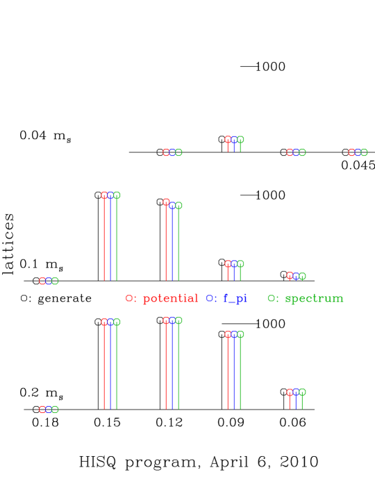
Figure 1: Status of the HISQ configuration generation program as of June 2010. We expect to eventually bring all these ensembles to approximately 1000 equilibrated configurations. The ensembles at the physical quark mass ($0.04\,m_{s}$) at $a=0.06$ and $0.045$ fm will require next generation computers. The black bars show the number of equilibrated configurations, and the red, blue and green bars show the progress of static potential, light pseudoscalar amplitudes, and simple hadron spectrum calculations. These are being done in parallel with the configuration generation to the extent possible.

During the past eleven years the MILC collaboration has carried out a program of QCD simulations using an improved staggered quark action, the “asqtad” action. This action has lattice artifacts that are much smaller than those in the original (one-link) staggered quark action. These simulations used two light and one strange dynamical quarks. Lattices have been generated with spacings ranging from 0.18 fm to 0.045 fm and light quark masses ranging from 0.05 $m_{s}$ to $m_{s}$. The spatial sizes of these lattices ranged from 2.5 fm to 5.8 fm. In total, around 25000 configurations have been archived. These configurations have been used for a wide variety of QCD studies and are all publicly available from the NERSC Gauge Connection archive, from ILDG, or informally. A detailed review of this simulation program can be found in Ref. [1].

Recently the HPQCD/UKQCD collaboration introduced a “highly improved staggered quark” (HISQ) action which further reduces taste symmetry violations, which are expected to be the largest lattice artifacts with staggered quark actions. Using this action, and taking advantage of improved machine power and algorithm development, we have begun a new program of lattice QCD simulations. There are several differences between this new set of simulations and those in the asqtad program. First, the smeared links used in the $\makebox[0.0pt][l]{\,/}D$ operator are done with a two level smearing, so that the quarks effectively see a smoother lattice, leading to reduced taste symmetry violations. Second, the three-link (Naik) term in $\makebox[0.0pt][l]{\,/}D$ for the charm quark is modified to improve the dispersion relation of the free charm quark. These two improvements together make up what is usually called the HISQ action[2]. In addition, this generation of simulations is using spatial lattice sizes about 20% larger than the comparable asqtad action simulations. While this seems like a small adjustment, since finite size effects are expected to decrease as $\exp(-m_{\pi}L)$, these effects should be significantly reduced. Also, the Symanzik improved gauge action contains the one-loop effects of the HISQ fermions[3]. The comparable asqtad effects were not available when that program was started, but turned out to be surprisingly large[4]. With experience from the asqtad simulations, we expect to do a better job of tuning the dynamical quark masses, reaching a level of perhaps 2% accuracy. In contrast, some of the early asqtad lattice ensembles had strange quark masses as much as 20% off their a posteriori correct value. Finally, we are including a dynamical charm quark. At our smaller lattice spacings, $am_{c}$ is not large. We do expect the effects of dynamical charm to be small in most cases, but they may be important to the high temperature QCD part of our program, and they are quite cheap in include.

In this program we expect to produce full scale ensembles with about 1000 equilibrated configurations at lattice spacings of $0.15$, $0.12$, $0.09$ and $0.06$ fm, with light quark masses of $m_{s}/5$, $m_{s}/10$ and the physical value, roughly $m_{s}/27$. In the not too distant future we also expect to generate an ensemble with $a=0.045$ fm and the physical quark masses. We will also generate a number of coarser ensembles, mainly for setting the scale in HISQ high temperature QCD simulations. For each of these approximate lattice spacings we are using values of $10/g^{2}$ and $u_{0}$ determined from the $m_{l}=m_{s}/5$ runs at all light quark masses. The strange and charm quark masses are adjusted from short tuning runs to give the physical values of $2M_{K}^{2}-M_{\pi}^{2}$ and $\frac{3}{4}M_{\Psi}+\frac{1}{4}M_{\eta_{c}}$ respectively. Figure 1 shows the current (June 2010) status of these runs.

2 Tests of scaling

The first stage in this program was to generate complete ensembles at a fixed but unphysical light quark mass of $m_{s}/5$ at lattice spacings of $0.15$, $0.12$ and $0.09$ fm. This allows us to test scaling, or dependence of calculated quantities on the lattice spacing. In particular, we wish to see if the reductions in taste symmetry violations are accompanied by reductions in lattice spacing dependence of other quantities. The results of these tests are briefly summarized here, but a complete report may be found in Ref. [5].

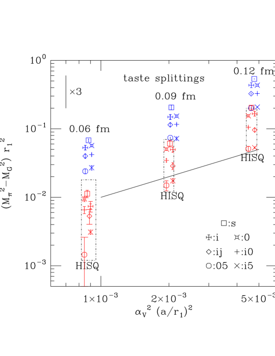
Figure 2: Taste splittings among the pions, comparing the asqtad and HISQ actions. The asqtad results used configurations with 2+1 flavors of dynamical quarks, and the HISQ results 2+1+1 flavors. The quantity plotted is $r_{1}^{2}\left(M_{\pi}^{2}-M_{G}^{2}\right)$, where $M_{\pi}$ is the mass of the non-Goldstone pion and $M_{G}$ is the mass of the Goldstone pion. Reading from top to bottom, the non-Goldstone pions are the $\pi_{s}$ (box), $\pi_{0}$ (fancy box), $\pi_{i}$ (fancy plus), $\pi_{io}$ (plus), $\pi_{ij}$ (diamond), $\pi_{i5}$ (cross) and $\pi_{05}$ (octagon). $r_{1}^{2}\left(M_{\pi}^{2}-M_{G}^{2}\right)$ is known to be almost independent of the light-quark mass. The vertical bar at the upper left shows the size of a factor of three, roughly the observed reduction in taste splittings, while the sloping solid line shows the theoretically expected dependence on lattice spacing. Nearly degenerate points have been shifted horizontally to improve their visibility.

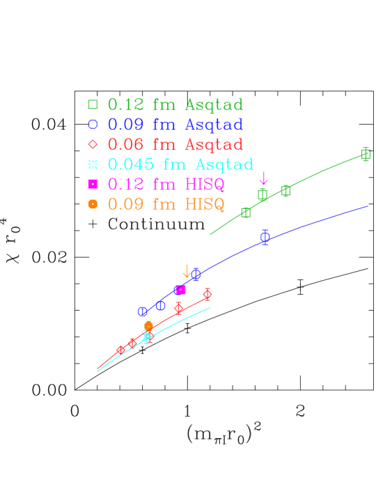
Figure 3: The topological susceptibility, comparing the asqtad and HISQ actions. Points with the asqtad action are shown for several lattice spacings and quark masses, and the HISQ results for $a\approx 0.12$ fm and $a\approx 0.09$ fm with $m_{l}=0.2m_{s}$. For the horizontal axis we use the mass of the taste singlet pion, since in lowest order chiral perturbation theory the topological susceptibility is a function of this mass [6]. The curves in the figure come from a chiral perturbation theory fit to the asqtad data. A discussion of the methods used for computing the susceptibility and the asqtad results can be found in Ref. [7]. The two arrows indicate the locations of asqtad points with lattice spacing and quark mass similar to the two HISQ points. (In the case of the $a\approx 0.09$ fm HISQ point, the quark mass falls between two of the masses of the asqtad points.)

The HPQCD/UKQCD collaboration demonstrated the reduction of taste violations with HISQ valence quarks using quenched and asqtad sea quarks[2]. As expected, we find similar results with HISQ sea quarks. Figure 2 shows results for the taste splittings with HISQ valence and sea quarks with $m_{l}=m_{s}/5$, including some results on a partially completed ensemble with $a=0.06$ fm.

Perhaps the most stringent test of improvement is the topological susceptibility, since the dependence of this quantity on the sea quark mass demonstrates that the sea quarks are modifying the gluon configurations. Figure 3 shows the topological susceptibility for most of the asqtad ensembles[7], together with the HISQ results for $m_{l}=m_{s}/5$ at $a=0.12$ and $0.09$ fm. It can be seen that the HISQ points fall below the corresponding asqtad points, which are indicated by the arrows in the figure. Note that the HISQ points are to the left of the corresponding asqtad points. This is because the horizontal axis is the mass of the taste singlet pion (the heaviest pion taste), and the reduction in taste symmetry breaking moves the points to the left. It is the movement down relative to the asqtad points that represents an improvement in the gluon configurations.

We also looked at the masses of the $\rho$ and nucleon in these ensembles. Strictly, these are an unphysical vector meson and baryon with both valence and sea light quark masses at $m_{s}/5$. Thus, we can check their dependence on lattice spacing, but without a chiral extrapolation we cannot test their masses against experiment. With this caution, we found that the dependence of $r_{1}M_{\rho}$ and $r_{1}M_{N}$ on the lattice spacing was much smaller than for the asqtad ensembles at comparable quark masses. More details are in Ref. [5]. Of course, this could be interpreted either as improved scaling of hadron masses using $r_{1}$ to set the scale or improved scaling of $r_{1}$ using hadron masses to set the scale.

3 Setting the length scale

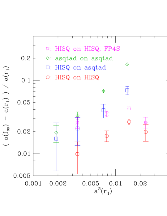
Figure 4: Differences in determinations of the length scale using different standards. In the legend, the symbol types are labelled as “valence on sea”. The “FP4S” points (bursts) use a pseudoscalar meson with both valence quarks at 0.4 times the strange quark mass, while all the other points use valence quarks at the strange quark mass. The “HISQ on asqtad” points are taken from Ref. [9].

QCD simulation programs involving unphysical quark masses generally involve a definition of the lattice spacing as a function of the gauge couplings and sea quark masses. About the only real requirement on this definition is that it should be correct at the physical quark masses in the continuum limit. The most common choice is a scale determined from the static quark potential[8], usually either $r_{0}^{2}F(r_{0})=-1.65$ or $r_{1}^{2}F(r_{1})=-1$. This is not a physical quantity, but it is a convenient interpolating quantity that can be determined accurately with a reasonable amount of work. Its value is determined by matching some physical quantity, such as quarkonium mass splittings or $f_{\pi}$, in the continuum and chiral limits. Recently the HPQCD collaboration has suggested using the decay constant of a fictitious isovector pseudoscalar meson with valence quark masses equal to the strange quark mass as the length standard[9], which we will call $f_{ss}$. Like $r_{0}$ or $r_{1}$, this is an unphysical quantity whose value is determined by matching a physical quantity, most likely $f_{\pi}$, in the continuum limit at the physical quark mass. Of course, one could use any mass for the valence quark, and we have been experimenting with using a mass of $0.4$ times the strange quark mass. The choice of reference mass involves a tradeoff — we want a mass heavy enough so that an accurate simulation result is possible but light enough so that chiral perturbation theory can be used with confidence.

Use of an unphysical decay constant has several advantages. It is possible to get very good accuracy, and the systematic errors from things like choices of fit ranges are better understood than those in $r_{1}$. Also, for calculations involving hadron masses and matrix elements, there are fewer steps in the logic relating the lattice results to dimensionful quantities. On the other hand, the meson decay constant takes much more computer time than the static quark potential (although it may be needed anyway) and is dependent on the choice of valence quark formulations. For example, asqtad and HISQ valence quarks would give different lattice spacings for the same ensemble of configurations.

Table 1 shows the lattice spacings for several asqtad and HISQ ensembles determined from $r_{1}$ and from pseudoscalar amplitudes with asqtad and HISQ valence quarks. Figure 4 shows the differences between the pseudoscalar and $r_{1}$ lattice spacings versus $a^{2}$, including lattice spacings determined from both $f_{ss}$ and $f_{.4s}$, and it can be seen that the differences are vanishing in the continuum limit.

Action	$10/g^{2}$	$am_{l}$	$am_{s}$	$am_{c}$	$a(r_{1})$	$a(f_{ss,\mathrm{asq}})$	$a(f_{ss,\mathrm{HISQ}})$
asqtad	6.76	0.01	0.05	–	0.1178(2)	0.1373(2)	0.1264 (11)
asqtad	7.09	0.0062	0.031	–	0.0845(1)	0.0905(3)	0.0878(7)
asqtad	7.46	0.0036	0.018	–	0.0588(2)	0.0607(1)	0.0601(5)
asqtad	7.81	0.0028	0.014	–	0.0436(2)	0.0444(1)	0.0443(4)
HISQ	5.80	0.013	0.065	0.838	0.1527(7)	na	0.1558(3)
HISQ	6.00	0.0102	0.0509	0.635	0.1211(2)	na	0.1244(2)
HISQ	6.30	0.0074	0.037	0.440	0.0884(2)	na	0.0900(1)

Table 1: Lattice spacing determinations by various methods. The values for HISQ valence quarks with asqtad sea quarks are taken from Ref. [9]. In the other cases, the errors are statistical only; they do not include the errors on the physical value of $r_{1}$ ($r_{1}=0.3108(15)({}_{-79}^{+26})$) or on the estimate of $f_{ss}$ in MeV, $f_{ss}=181.5(1.0)$ MeV[9].

- [1] A. Bazavov et al., Rev. Mod. Phys. 82, 1349 (2010), [arXiv:0903.3598].
- [2] E. Follana et al., Nucl. Phys. B (Proc. Suppl.) 129 and 130, 447 (2004), [arXiv:hep-lat/0311004]; E. Follana et al., Nucl. Phys. B. (Proc. Suppl.) 129 and 130, 384, 2004. [arXiv:hep-lat/0406021]; E. Follana et al. [HPQCD Collaboration and UKQCD Collaboration], Phys. Rev. D 75, 054502 (2007) [arXiv:hep-lat/0610092].
- [3] A. Hart, G. von Hippel and R.R. Horgan, Phys. Rev. D 79, 074008 (2009), [arXiv:0812.0503].
- [4] Zh. Hao et al. Phys. Rev. D76, 034507 (2007), [arXiv:0705.4660].
- [5] A. Bazavov et al., Phys. Rev. D 82, 074501 (2010), [arXiv:1004.0342].
- [6] C. Aubin and C. Bernard, Phys. Rev. D68, 034014, (2003), [arXiv hep-lat/0304014]; B. Billeter, C.E. DeTar and J. Osborn, Phys. Rev. D70, 077502, (2004), [arXiv hep-lat/0406032].
- [7] A. Bazavov et al., Phys. Rev. D81, 114501 (2010), [arXiv:1003.5695].
- [8] R. Sommer, Nucl. Phys. B411, 839 (1994), [arXiv:hep-lat/9310022].
- [9] C.T.H. Davies et al., Phys. Rev. D 81, 034506 (2010), [arXiv:0910.1229].