Dust and Chemical Abundances of the Sagittarius dwarf Galaxy Planetary Nebula Hen2-436

Abstract

We have estimated elemental abundances of the planetary nebula Hen2-436 in the Sagittarius (Sgr) spheroidal dwarf galaxy using ESO/VLT FORS2, Magellan/MMIRS, and $Spitzer$/IRS spectra. We have detected candidates of fluorine [F ii]$\lambda$4790, krypton [Kr iii]$\lambda$6826, and phosphorus [P ii]$\lambda$7875 lines and successfully estimated the abundances of these elements ([F/H]=+1.23, [Kr/H]=+0.26, [P/H]=+0.26) for the first time. These elements are known to be synthesized by neutron capture process in the He-rich intershell during the thermally pulsing AGB phase. We present a relation between C, F, P, and Kr abundances among PNe and C-rich stars. The detections of F and Kr in Hen2-436 support the idea that F and Kr together with C are synthesized in the same layer and brought to the surface by the third dredge-up. We have detected N ii and O ii optical recombination lines (ORLs) and derived the N²⁺ and O²⁺ abundances. The discrepancy between the abundance derived from the oxygen ORL and that derived from the collisionally excited line is $>$1 dex. To investigate the status of the central star of the PN, nebula condition, and dust properties, we construct a theoretical spectral energy distribution (SED) model to match the observed SED with Cloudy. By comparing the derived luminosity and temperature of the central star with theoretical evolutionary tracks, we conclude that the initial mass of the progenitor is likely to be $\sim$1.5-2.0 $M_{\odot}$ and the age is $\sim$3000 yr after the AGB phase. The observed elemental abundances of Hen2-436 can be explained by a theoretical nucleosynthesis model with a star of initial mass 2.25 $M_{\odot}$, $Z$=0.008 and LMC compositions. We have estimated the dust mass to be 2.9$\times$10^-4 $M_{\odot}$ (amorphous carbon only) or 4.0$\times$10^-4 $M_{\odot}$ (amorphous carbon and PAH). Based on the assumption that most of the observed dust is formed during the last two thermal pulses and the dust-to-gas mass ratio is 5.58$\times$10^-3, the dust mass-loss rate and the total mass-loss rate are $<$3.1$\times$10^-8 $M_{\odot}$ yr^-1 and $<$5.5$\times$10^-6 $M_{\odot}$ yr^-1, respectively. Our estimated dust mass-loss rate is comparable to a Sgr dwarf galaxy AGB star with similar metallicity and luminosity.

1. Introduction

Currently, $>$5,000 objects are regarded as planetary nebulae (PNe) in the local group galaxies. Of them, BoBn1 (Otsuka et al. 2008; Otsuka et al. 2010), Wray16-423, StWr2-21 (Kniazev et al. 2008; Zijlstra et al. 2006), and Hen2-436 (Walsh et al. 1997; Dudziak et al. 2000; this paper) belong to the Sagittarius (Sgr) dwarf galaxy. Sgr dwarf galaxy PNe are interesting objects as they provide direct insight into old, low-mass stars and also information on the history of the Galactic halo. In some galactic evolution scenarios, the galactic halo is partly built up from the tidal destruction and assimilation of dwarf galaxies. Sgr dwarf galaxy PNe are ideal laboratories and appropriate references to study the evolution of metal-deficient stars found in the Galactic halo and low-mass stars ($\lesssim$3.5 $M_{\odot}$) in the LMC. The metallicity of Sgr dwarf galaxy PNe is relatively low, e.g., $<$0.01 $Z_{\odot}$ in BoBn1 or $\sim$0.5 $Z_{\odot}$ in the others, which is equal to the typical metallicity of the LMC, and all the Sgr dwarf galaxy PNe are C-rich ([C/O]$\gtrsim 0$; e.g., Zijlstra et al. 2006) based on gas-phased C and O abundances. The Sgr dwarf galaxy PNe and LMC PNe would complement each other in a study of metal-deficient PNe. In addition, since the distance to the Sgr dwarf galaxy is well determined (24.8 kpc; Kunder & Chaboyar 2009) and the interstellar reddening to the Sgr dwarf galaxy PNe is relatively low ($E(B-V)$ $\lesssim$0.1), we can accurately estimate intrinsic flux densities. Moreover, by using the spatially highly resolved images taken by Hubble Space Telescope ($HST$) and 8-m class ground based telescopes, we can estimate the size and shape of the nebulae. The nebular size is an important parameter in building spectral energy distributions (SED). We have collected data on several Sgr dwarf galaxy PNe to investigate elemental abundances, dust mass, and evolutionary status of the central star in a metal-deficient environment. In this paper, we analyze the most recently secured spectral data of the Sgr dwarf galaxy PN Hen2-436 (PN G004.8–22.7).

Hen2-436 is an interesting object in terms of chemical abundances and dust production in metal-poor environments. Zijlstra et al. (2006) argued that dust exists within the nebula. Sterling et al. (2009) detected [Kr iii]$\lambda$2.19 $\mu$m and [Se iv]$\lambda$2.29 $\mu$m lines in the Gemini/GNIR spectra, although the amounts of these elements are not estimated yet. In the extra-Galactic PNe, these slow neutron capture elements (s-process elements) have so far only been detected in BoBn1 (Otsuka et al. 2010) and this nebula. The detection of such rare elements in PNe is highly interesting.

For Hen2-436, we performed a comprehensive chemical abundance analysis based on optical ESO/VLT FORS2 spectra, near-IR spectra from Magellan/MMIRS, and mid-IR $Spitzer$/IRS spectra. From FORS2 spectra, we found candidate detections of fluorine (F), phosphorus (P), and krypton (Kr) forbidden lines, and we estimate abundances of these elements. The estimations of F and P are done for the first time. Both elements are synthesized by neutron capture in the He-rich intershell of AGB stars. Through spectral energy distribution (SED) modeling with the photo-ionization code Cloudy (Ferland 2004), we infer the evolutionary status of the central star and try to estimate the dust mass. We further investigate the evolutionary status of the progenitors of Hen2-436 and the other Sgr dwarf galaxy PNe with similar metallicity. The observed chemical abundances are compared with theoretical nucleosynthesis model predictions.

2. Data and Reduction

2.1. VLT/FORS2 Archive Data

The optical low-dispersion spectra of Hen2-436 in the range 3320 Å to 8620 Å are available from the European Southern Observatory (ESO) archive. The observations were performed by M.Pẽna (Prop. I.D.: 077.B-0430B) on August 23th, 2006, using the visual and near UV FOcal Reducer and low dispersion Spectrograph 2 (FORS2; Appenzeller et al. 1998) at the Cassegrain focus of the ANTU, one of the four 8.2-m telescopes of the ESO Very Large Telescope (VLT) at Paranal, Chile. The entrance slit size was 417$\farcs 79$ in length and 1$\farcs 01$ in width. The position angle (P.A.) was set to 0^∘. The 2$\times$2 on-chip binning pattern was chosen, hence the sampling pitch was $\sim$1.4 Å pixel^-1 in wavelength and 0$\farcs 5$ pixel^-1 in space. By measuring the FWHM ($\sim$4.7 Å) of sky lines around 5500 Å, we determine the spectral resolving power $R$ ($\lambda$/$\Delta\lambda$) to be $\sim$1200. The data were taken by long (3$\times$60 sec) and short (3$\times$ 1, 5, and 10 sec) exposures. In order to measure the fluxes for strong lines such as [O iii] and H$\alpha$, we used the short exposure frames, and for weak line measurements we used the long exposure frames. The seeing was $\sim$1$\farcs 0$ during the exposure. The standard star LTT7987 was observed for flux calibration and telluric absorption correction. For wavelength calibration, we used He-Hg-Cd lamp frames and night sky-lines recorded in the object frames.

Data reduction and emission line analysis were performed mainly with a long-slit reduction package noao.twodspec in IRAF. Data reduction was performed in a standard manner. In measuring the fluxes of emission-lines, we assumed that the line profiles were all Gaussian and we applied multiple Gaussian fitting techniques.

In the panels (a), (b), (c), and (d) of Figure 1, we present the FORS2 spectra. The vertical axis is the scaled flux density in units of Å^-1, normalized to the H$\beta$ flux $F$(H$\beta$)=1000, and the horizontal axis is the rest wavelength. We also present candidate detections of fluorine [F ii]$\lambda$4790, krypton [Kr iii]$\lambda$6826, and phosphorus [P ii]$\lambda$7875 lines.

2.2. Magellan/MMIRS Observation

We performed $J$ band (1.17-1.33 $\mu$m) moderate-resolution spectroscopy using the MMT and Magellan Infrared Spectrograph (MMIRS; McLeod et al. 2004) at the Cassegrain focus of the Magellan Clay 6.5-m telescope on April 27th, 2010 (PI.: M.Meixner). The detector of MMIRS is a 2048$\times$2048 pixel Hg-Cd-Te Hawaii-II array. The entrance slit size was 420^′′ in length and 1^′′ in width. The P.A. was set to 0^∘. The sampling pitch is $\sim$2.5$\times$10^-4 $\mu$m pixel^-1 in wavelength and 0$\farcs 2$ pixel^-1 in space. We determine $R$ to be $\sim$1400 by measuring the FWHM ($\sim$8.5$\times$10^-4 $\mu$m) of night sky-lines around 1.23 $\mu$m. We observed Hen2-436 and the standard star HIP94663 (A0V, 2MASS $J$=7.425) using a three-point dither pattern for sky background subtraction. The total exposure time for Hen2-436 is 900 sec (3$\times$300 sec). The seeing was $\sim$1^′′ during the exposure. For wavelength calibration, we used night sky-lines recorded in the object frames. Data reduction was performed using IRAF. The telluric absorption and flux calibration were corrected using the HIP94663 frames. The MMIRS spectrum s presented in Figure 1(e). The strong emission lines are He i + Pa$\beta$ $\lambda$1.28$\mu$m.

2.3. Spitzer/IRS Archive Data

We used the data set of program ID: P30333 (PI: A.Zijlstra) taken by the Spitzer space telescope on October 18th, 2006. The data were taken with the Infrared Spectrograph (IRS, Houck et al. 2004) using the SL (5.2-14.5 $\mu$m) and LL (14-38$\mu$m) modules. Due to the low signal-to-noise ratio, the SL data were not available for chemical abundance analysis and SED modeling. The one-dimensional spectra were extracted using spice version c15.0A. We extracted the region within $\pm$1^′′ from the center of each spectral order and summed along the spatial direction. No correction for interstellar extinction was made since it is negligibly small in this IR wavelength band. In Figure 1(f) we present the extracted Spitzer spectrum. We detected the [Ne iii] $\lambda$15.5$\mu$m fine-structure line. The spectrum shows a broad emission feature to the red of the [Ne iii] $\lambda$15.5 $\mu$m line. Since Hen2-436 is considered to be a C-rich PN, the feature might be related to the C-C-C PAH bending modes, which are observed in some Magellanic Cloud PNe (Bernard-Salas et al. 2009). It should be noted, however, that to date, the C and O abundances of Hen2-436 have only been derived from different types of emission lines; the C and O abundances are from recombination and from forbidden lines, respectively. There are no UV spectra available from which to estimate the C²⁺ abundances using the C iii] $\lambda\lambda$1906/09 lines. Cohen & Barlow (2005) found that the PAH 7.7 $\mu$m band is detectable in PNe with C/O $>$ 0.56${}_{-0.41}^{+0.21}$ based on ISO/SWS spectra of over 40 PNe. To verify whether Hen2-436 has PAHs, we need to check the C/O ratio based on the C and O abundances from the same type of emission lines.

2.4. $HST$/WFPC2 Archive Data

The archival $HST$/WFPC2 images taken with the F502N ($\lambda_{c}$=5013 Å/$\Delta\lambda$=35.8 Å), F547M (5484 Å/638 Å), and F656N (6564 Å/28 Å) filters are publicly available. These images were taken by A.Zijlstra (Proposal I.D.: 9356) on May 4th, 2003. The WFPC2 frames reduced and calibrated by the $HST$ pipeline (including MultiDrizzle), were downloaded from the $HST$ archive at the Canadian Astronomy Data Centre (CADC). In Figure 2 we present the intensity contour map overlaid on top of the F656N image. Hen2-436 has an elongated nebula along P.A.=90^∘. We performed aperture photometry to estimate the amount of light passing through the slit and to do flux correction (see below). We measured the total flux within a 1^′′ radius and subtracted the background from an annulus centered on the PN with inner and outer radii of 1.1^′′ and 1.3^′′. We performed aperture corrections using point spread functions generated by the TinyTim software package. For F547M, we assumed a 9000 K blackbody function as the incident SED. The measured fluxes are listed in Table 2. $X(-Y)$ means $X\times 10^{-Y}$ hereafter. The uncertainty corresponds to the standard deviation of the background. To estimate the contributions from both the stellar and nebular continuum to F502N and F656N, we measured the total emission line flux in the F547M band using the FORS2 spectra. Since the total emission line flux in the F547M band is 2.34(–13) $\pm$ 1.85(–14) erg s^-1 cm^-2, about half of the total flux could originate from the continuum. Using the averaged continuum flux density in the F547M, we estimated the stellar and nebular continuum subtracted [O iii] and H$\alpha$ fluxes to be 5.29(–12) and 2.39(–12) erg s^-1 cm^-2, respectively.

The observation logs for Hen2-436 are summarized in Table 1.

Figure 1.— (panels a, b, c, and d) the FORS2 spectrum of Hen2-436. The vertical axis is the scaled flux density in unit of Å^-1 which is normalized to the H$\beta$ flux $F$(H$\beta$)=1000. (panels e and f) the MMIRS and $Spitzer$ spectrum of Hen2-436. The vertical axis is the scaled flux density in units of $\mu$m^-1 which is normalized to the $F$(H$\beta$)=1.

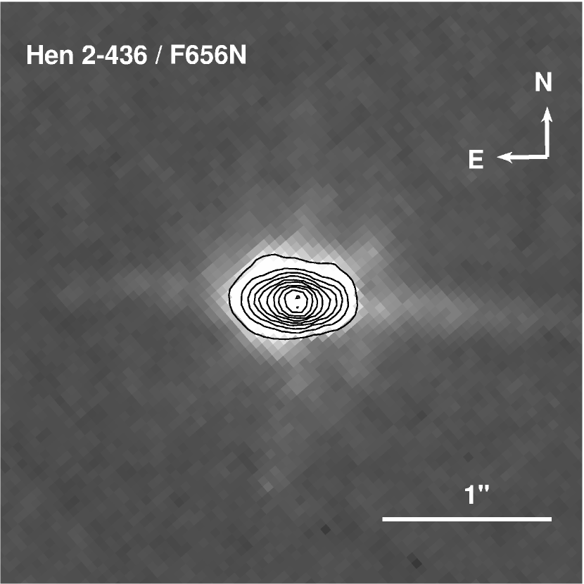
Figure 2.— The intensity contour map on the $HST$/WFPC2 F656N (H$\alpha$) image.

Table 1Observation logs for Hen2-436

Obs. Date	Telescopes/Instruments	Wavelength or	Exp.Time
		Filter
2006/08/23	VLT/FORS2	3320–8620 Å	3$\times$60,10,5,1 sec
2010/04/27	Magellan/MMIRS	1.17-1.33 $\mu$m	3$\times$300 sec
2006/10/18	Spitzer/IRS	14-38 $\mu$m	2$\times$14.68 sec
2003/05/04	HST/WFPC2	F502N	2$\times$80 sec
		F547M	1$\times$60 sec
		F656N	2$\times$100 sec

Table 2The fluxes measured from the $HST$ images.

Filter	$\lambda_{c}$	Flux
	(Å)	(erg s-1 cm-2)
F502N	5013	5.38(–12) $\pm$ 7.96(–14)
F547M	5484	5.69(–13) $\pm$ 6.06(–14)
F656N	6564	2.43(–12) $\pm$ 3.04(–14)

3. Results

3.1. Detected Lines and Interstellar Reddening Correction

We have detected over 100 lines, including useful lines to investigate plasma diagnostics and estimate ionic abundances. We estimate ionic abundances using detected optical recombination lines (ORLs) and collisionally excited lines (CELs).

Before performing plasma diagnostics and chemical abundance analysis, we corrected our measured fluxes for interstellar reddening by determining the reddening coefficient at H$\beta$, $c$(H$\beta$). We compared the observed line ratio of H$\alpha$ to H$\beta$ to the theoretical ratio computed by Storey & Hummer (1995) assuming a temperature $T_{\epsilon}$ = 10⁴ K a density $n_{\epsilon}$ = 10⁴ cm^-3 and a nebula optically thick to Ly-$\alpha$ (Case B of Baker & Menzel 1938). From this we estimate $c$(H$\beta$) = 0.23 $\pm$ 0.05. From Seaton’s (1979) relation $c$(H$\beta$) = 1.47$E(B-V)$ one obtains $E(B-V)$ = 0.16 $\pm$ 0.03, which agrees fairly well with the value (0.13) measured in the direction of Hen2-436 in the Galactic extinction map of Schlegel et al. (1998).

All of the line fluxes in optical to near-IR were de-reddened using the formula:

$$\log_{10}\left[\frac{I(\lambda)}{I{\rm(H\beta)}}\right]=\log_{10}\left[\frac{F(\lambda)}{F{\rm(H\beta)}}\right]+c({\rm H\beta})f(\lambda),$$ (1)

where $I(\lambda)$ and $F(\lambda)$ are the de-reddened and the observed fluxes at $\lambda$, respectively, and $f(\lambda)$ is the interstellar extinction at $\lambda$, computed by the reddening law of Cardelli et al. (1989) with $R_{V}$ = 3.1. Comparing the observed [O iii]$\lambda$5007, the H$\alpha$ fluxes from the FORS2 observation and the continuum subtracted F507N and F656N fluxes, we estimate 83$\%$ of the total flux from Hen2-436 to be passing through the $1.^{\prime\prime}0$ width slit entrance of FORS2. We estimate the total H$\beta$ flux to be 6.37(–13) $\pm$ 9.76(–15) erg s^-1 cm^-2. Our measured value is consistent with Cahn et al. (1992), $\log_{10}F(H\beta)$ = –12.02 $\pm$ 0.03. Using $c$(H$\beta$), we estimate the de-reddened total H$\beta$ flux to be 1.08(–12) $\pm$ 1.46(–13) erg s^-1 cm^-2.

The de-reddened emission line fluxes detected in the FORS2, MMIRS, and IRS spectra are listed in Table 3. These line fluxes are normalized to $I$(H$\beta$)=100. In the columns of laboratory wavelength ($\lambda_{\rm lab}$), we indicate the stellar origin lines by the asterisks ($\ast$). These stellar lines have the wide FWHM, typically, $\gtrsim$ 8 Å. Thanks to the large photon collecting power of VLT/FORS2, we detected 192 emission lines in total, including many weak intensity recombination lines of C, N, and O. Our measurements largely improved over previous detections by Welsh et al. (1997), who detected 51 emission lines in ESO NTT 3.5-m/EMMI (spectral resolution 4.5 Å) and ESO 1.5-m/Boller and Chievens spectra (5-7 Å). The normalized line fluxes $I$($\lambda$) of Welsh et al. (1997) and our measurements agree within 2 $\%$.

3.2. Plasma Diagnostics

3.2.1 CELs Plasma Diagnostics

We have detected several collisionally excited lines (CEL) useful for estimations of the electron temperatures ($T_{\epsilon}$) and densities ($n_{\epsilon}$). We have examined the electron temperature and density structure within the nebula using 8 diagnostic CEL ratios. Electron temperature and density were derived from each diagnostic ratio for each line combination by solving for the level populations in a multi-level ($>$ 5 for most ions) atomic model using the collision strengths $\Omega_{ij}$ ($j$$>$$i$) and spontaneous transition probabilities $A_{ji}$ for each ion. The estimated electron temperatures and densities are listed in Table 4. We used the same atomic data as in Otsuka et al. (2010). A diagnostic diagram that plots the loci of the observed diagnostic line ratios on the log($n_{\epsilon}$)-$T_{\epsilon}$ plane is shown in Figure 3. The solid lines indicate diagnostics of the electron temperature, and the broken lines are electron density diagnostics. This diagram shows that most of the CELs having ionization potentials (I.P.) $>$ 13.5 eV are emitted from $T_{\epsilon}\sim$10 000–14 000 K and $n_{\epsilon}\sim$80 000–200 000 cm^-3 ionized gas. In such a high density nebula, [S ii] and [O ii] diagnostic line ratios do not give reliable $T_{\epsilon}$ due to the low critical density of [S ii]$\lambda\lambda$6716/31 and [O ii]$\lambda$3727 lines. Hence, these diagnostic lines were used only for density derivation. Meanwhile, the [N ii], [O iii], [Ne iii], and [Ar iii] diagnostic lines can be used as reliable $T_{\epsilon}$ indicators.

For [N ii]$\lambda$5755 and [O ii]$\lambda\lambda$7320/30, we need to consider the recombination contamination from N²⁺ and O²⁺ lines. We subtracted this contamination using Equations (2) and (3) given by Liu et al. (2000),

$$\frac{I_{R}(\rm[N\,{\sc II}]\lambda 5755)}{I(\rm H\beta)}=3.19\left(\frac{T_{\epsilon}}{10^{4}}\right)^{0.33}\times\frac{\rm N^{2+}}{\rm H^{+}},$$ (2)

$$\frac{I_{R}(\rm[O\,{\sc II}]\lambda\lambda 7320/30)}{I(\rm H\beta)}=9.36\left(\frac{T_{\epsilon}}{10^{4}}\right)^{0.44}\times\frac{\rm O^{2+}}{\rm H^{+}}.$$ (3)

where N²⁺/H⁺ and O²⁺/H⁺ are the doubly ionized nitrogen and oxygen abundances, respectively. Adopting the value derived from optical recombination line (ORL) analysis (see Section 3.3.2), we estimate $I_{R}$([N ii] $\lambda$5755) $\sim$0.2, which is approximately 22 $\%$ of the observed value. Likewise, we estimated $I_{R}$([O ii] $\lambda\lambda$7320/30) $\gtrsim$2.9, which is approximately $\gtrsim$25 $\%$ of the observed value.

First, we calculated the electron density. We adopted a constant temperature of 12 000 K for the calculations of $n_{\epsilon}$([S ii]) and $n_{\epsilon}$([O ii]), and 14 000 K when calculating $n_{\epsilon}$([Cl iii]) and $n_{\epsilon}$([Ar iv]). Next, we calculated the electron temperature. $T_{\epsilon}$([N ii]) was calculated assuming a density of $n_{\epsilon}$([O ii]), $T_{\epsilon}$([Ar iii]) was using $n_{\epsilon}$([Cl iii]), and $T_{\epsilon}$([Ne iii]) and $T_{\epsilon}$([O iii]) were using $n_{\epsilon}$([Ar iv]). The resultant $n_{\epsilon}$ and $T_{\epsilon}$ are listed in Table 4.

3.2.2 ORLs Plasma Diagnostics

We detected optical recombination lines (ORLs) of He, C, N, and O. To calculate ionic abundances of these elements using ORLs, we estimated the electron temperature from the Balmer discontinuity and He i line ratios. We used the same atomic data employed by Otsuka et al. (2010).

The electron temperature derived by these two methods are listed in Table 4. The Balmer discontinuity electron temperature $T_{\epsilon}$(BJ) of 14 500 $\pm$ 2200 K was estimated using the equation given in Liu et al. (2001).

Using four diagnostic He i line ratios, the He i electron temperature $T_{\epsilon}$(He i) was estimated assuming a constant electron density $n_{\epsilon}$ = 10⁵ cm^-3. All the He i lines we chose for the $T_{\epsilon}$(He i) derivation are insensitive to electron density. We adopted the emissivities of He i lines from Benjamin et al. (1999). We consider that the $T_{\epsilon}$(He i) from the $\lambda$7281/$\lambda$6678 ratio is the most reliable value because (i) He i $\lambda$6678 and $\lambda$7281 are from levels having the same spin as the ground state and the Case B recombination coefficients for these lines by Benjamin et al. (1999) are more certain than those for $\lambda$4471 and $\lambda$5876; (ii) the interstellar extinction is less of a complication due to the similar wavelengths of these lines. Thus, we adopted $T_{\epsilon}$(He i) derived from the He i $\lambda$7281/$\lambda$6678 ratio for the He⁺ abundance calculation.

Table 3The line list of Hen 2-436 detected in the FORS2/MMIRS/IRS observations.

$\lambda_{\rm lab}$	Ion	$f$($\lambda$)	$I$(H$\beta$)	$\delta I$(H$\beta$)	$\lambda_{\rm lab}$	Ion	$f$($\lambda$)	$I$(H$\beta$)	$\delta I$(H$\beta$)	$\lambda_{\rm lab}$	Ion	$f$($\lambda$)	$I$(H$\beta$)	$\delta I$(H$\beta$)
3498.77	He i	0.367	0.516	0.371	5131.25	[Kr v]?	–0.068	0.081	0.022	7099.80	[Pb ii]?	–0.369	0.075	0.006
3587.28	He i	0.349	0.659	0.180	5145.17	C ii	–0.071	0.074	0.017	7113.04	C ii	–0.371	0.053	0.008
3634.24	He i	0.341	0.668	0.102	5172.34	N ii	–0.077	0.015	0.008	7135.80	[Ar iii]	–0.374	7.664	0.385
3643.93	Ne ii	0.339	0.394	0.214	5179.90	C iii	–0.078	0.010	0.013	7160.61	He i	–0.377	0.078	0.016
3679.35	H i	0.332	0.123	0.110	5191.82	[Ar iii]	–0.081	0.063	0.005	7170.50	[Ar iv]	–0.378	0.035	0.006
3682.81	He i	0.331	0.182	0.108	5197.90	[N i]	–0.082	0.142	0.007	7231.34	C ii	–0.387	0.345	0.039
3686.83	H i	0.330	0.436	0.173	5259.06	C ii	–0.095	0.029	0.005	7236.42	C ii	–0.387	0.559	0.036
3691.55	H i	0.329	0.643	0.118	5261.19	N ii	–0.096	0.051	0.017	7254.15	O i	–0.390	0.182	0.022
3697.15	H i	0.328	0.713	0.151	5270.40	[Fe iii]	–0.098	0.079	0.011	7262.70	[Ar iv]	–0.391	0.043	0.021
3704.98	He i	0.327	1.786	0.134	5335.65	[Fe ii]	–0.111	0.042	0.004	7281.35	He i	–0.393	1.329	0.064
3711.97	H i	0.325	1.407	0.110	5344.31	Fe iii	–0.113	0.108	0.009	7298.04	He i	–0.395	0.064	0.038
3721.94	H i	0.323	2.041	0.158	5376.19∗	C iii	–0.119	0.797	0.052	7319.46	[O ii]	–0.398	8.293	0.404
3726.03	[O ii]	0.322	9.249	0.424	5403.40	C ii	–0.124	0.054	0.006	7330.20	[O ii]	–0.400	6.746	0.354
3734.37	H i	0.321	2.241	0.157	5426.70	[Fe iii]	–0.129	0.046	0.003	7468.31	N i	–0.418	0.016	0.011
3750.15	H i	0.317	3.066	0.164	5470.68 ∗	C iv	–0.136	0.066	0.006	7499.85	He i	–0.422	0.059	0.005
3759.88	O iii	0.315	0.351	0.118	5471.10∗	C iv	–0.137	0.097	0.009	7499.85	He i	–0.422	0.067	0.010
3770.63	H i	0.313	3.947	0.171	5480.05	N ii	–0.139	0.046	0.003	7530.80	C ii	–0.427	0.101	0.012
3784.89	He i	0.310	0.214	0.147	5488.46	C ii	–0.140	0.034	0.002	7725.90∗	C iv	–0.452	0.771	0.094
3797.90	H i	0.307	5.126	0.216	5512.77	O i	–0.144	0.045	0.005	7751.10	[Ar iii]	–0.455	1.842	0.099
3819.60	He i	0.302	1.554	0.451	5517.66	[Cl iii]	–0.145	0.057	0.007	7816.14	He i	–0.464	0.083	0.007
3835.38	H i	0.299	7.821	0.505	5537.89	[Cl iii]	–0.149	0.160	0.014	7816.14	He i	–0.464	0.083	0.007
3868.77	[Ne iii]	0.291	53.568	1.974	5543.47	N ii	–0.150	0.025	0.002	7875.99	[P ii]	–0.471	0.042	0.008
3889.05	H i	0.286	17.481	0.830	5552.68	N ii	–0.151	0.034	0.003	8046.30	[Cl iv]	–0.492	0.165	0.012
3920.68	C ii	0.279	0.175	0.055	5577.34	[O i]	–0.156	0.239	0.011	8196.50	C iii	–0.510	0.046	0.006
3926.54	He i	0.277	0.181	0.046	5602.44	[K vi]	–0.160	0.074	0.009	8203.93	He i	–0.511	0.062	0.011
3970.07	H i	0.266	30.116	1.037	5592.37∗	O iii	–0.164	0.032	0.008	8214.50	C iii	–0.513	0.051	0.007
4026.18	He i	0.251	2.564	0.212	5754.64	[N ii]	–0.185	0.918	0.120	8236.79∗	He ii	–0.515	0.027	0.008
4068.60	[S ii]	0.239	2.067	0.245	5794.88	He ii	–0.191	3.528	0.999	8240.19	H i	–0.516	0.044	0.005
4076.35	[S ii]	0.237	0.811	0.226	5811.97∗	C iv	–0.193	10.124	1.300	8260.93	H i	–0.518	0.019	0.004
4101.73	H i	0.229	23.668	0.726	5875.62	He i	–0.203	19.558	0.546	8264.62	He i	–0.518	0.033	0.003
4120.81	He i	0.224	0.479	0.282	5889.79	C ii	–0.205	0.030	0.002	8271.93	H i	–0.519	0.003	0.001
4143.76	He i	0.217	0.376	0.275	5896.78	He ii	–0.206	0.015	0.009	8276.31	H i	–0.520	0.000	0.000
4229.27	[Fe v]?	0.191	0.137	0.032	5910.58	[Fe ii]	–0.208	0.008	0.005	8281.12	H i	–0.520	0.019	0.009
4267.15	C ii	0.179	1.102	0.032	5927.82	N ii	–0.211	0.016	0.004	8286.43	H i	–0.521	0.029	0.012
4292.21	O ii	0.172	0.040	0.024	5931.83	He ii	–0.211	0.026	0.003	8292.31	H i	–0.521	0.043	0.009
4340.46	H i	0.156	46.149	1.177	5958.38	O i	–0.215	0.070	0.011	8298.83	H i	–0.522	0.070	0.009
4363.21	[O iii]	0.149	13.901	0.502	5977.03	He ii	–0.218	0.034	0.009	8305.90	H i	–0.523	0.103	0.011
4387.93	He i	0.141	0.671	0.039	5998.71	[Cu iii]	–0.221	0.027	0.007	8312.10	C iii	–0.524	0.125	0.010
4414.90	O ii	0.133	0.084	0.029	6046.23	O i	–0.228	0.056	0.004	8323.42	H i	–0.525	0.181	0.014
4439.71	[Fe ii]	0.125	0.333	0.028	6101.79	[K iv]	–0.235	0.031	0.005	8333.78	H i	–0.526	0.209	0.015
4471.47	He i	0.115	5.911	0.150	6118.26	He ii	–0.238	0.030	0.006	8345.55	H i	–0.527	0.249	0.017
4571.10	Mg i]	0.084	0.224	0.021	6141.70	Ba ii?	–0.241	0.018	0.006	8359.00	H i	–0.529	0.408	0.027
4634.12∗	N iii	0.065	0.877	0.040	6151.27	C ii	–0.242	0.050	0.008	8374.48	He i	–0.531	0.294	0.019
4640.64∗	N iii	0.063	0.713	0.034	6159.12	[Mn iii]	–0.244	0.018	0.010	8397.42	He i	–0.533	2.058	0.139
4650.25∗	C iii	0.060	1.679	0.050	6300.30	[O i]	–0.263	5.523	0.197	8413.32	H i	–0.535	0.328	0.058
4658.64∗	C iv	0.058	1.439	0.050	6312.10	[S iii]	–0.264	1.634	0.092	8421.67	He ii	–0.536	0.020	0.003
4665.86∗	C iii	0.056	0.948	0.046	6346.97	Mg ii	–0.269	0.034	0.007	8437.95	H i	–0.537	0.383	0.047
4673.73	O ii	0.053	0.522	0.032	6363.78	[O i]	–0.271	1.829	0.069	8444.55	He i	–0.538	1.430	0.113
4676.23	O ii	0.052	0.339	0.029	6461.71	N ii	–0.284	0.159	0.010	8467.25	H i	–0.540	0.428	0.028
4687.55	[Fe ii]	0.049	0.564	0.027	6548.04	[N ii]	–0.296	3.589	0.154	8480.79	He i	–0.542	0.023	0.017
4713.17	He i	0.042	1.379	0.028	6562.77	H i	–0.298	285.000	11.874	8486.29	He i	–0.543	0.024	0.020
4740.17	[Ar iv]	0.034	0.725	0.019	6583.46	[N ii]	–0.300	10.915	0.504	8500.32	[Cl iii]	–0.544	0.110	0.029
4756.59	[Mn iii]	0.029	0.043	0.031	6678.15	He i	–0.313	4.923	0.194	8502.48	H i	–0.544	0.428	0.037
4789.45	[F ii]	0.020	0.106	0.018	6716.44	[S ii]	–0.318	0.488	0.053	8519.35∗	He ii	–0.546	0.030	0.013
4802.58	Ne ii	0.016	0.088	0.020	6730.81	[S ii]	–0.320	1.098	0.058	8528.97	He i	–0.547	0.052	0.014
4861.33	H i	0.000	100.000	2.165	6779.94	C ii	–0.326	0.050	0.007	8545.38	H i	–0.549	0.544	0.035
4921.93	He i	–0.016	1.649	0.041	6791.47	C ii	–0.328	0.067	0.011	8566.92	He ii	–0.551	0.005	0.006
4931.23	[O iii]	–0.019	0.151	0.008	6800.68	C ii	–0.329	0.018	0.004	8581.88	He i	–0.552	0.117	0.014
4958.91	[O iii]	–0.026	265.073	6.368	6826.38	[Kr iii]	–0.333	0.036	0.005	8598.39	H i	–0.554	0.592	0.039
5006.84	[O iii]	–0.038	792.066	16.075	6907.80	[Fe iii]	–0.343	0.058	0.017	8616.95	[Fe ii]	–0.556	0.021	0.012
5041.26	O ii	–0.046	0.052	0.033	6933.89	He i	–0.347	0.016	0.007	1.253$\mu$m	[Fe ii]	–0.759	0.442	0.133
5047.74	He i	–0.048	0.262	0.018	6989.46	He i	–0.354	0.018	0.007	1.279$\mu$m	He i	–0.767	1.129	0.212
5114.06	O v	–0.063	0.070	0.026	7001.90	O i	–0.356	0.035	0.005	1.282$\mu$m	H i	–0.767	16.183	1.730
5121.83	C ii	–0.065	0.080	0.053	7065.18	He i	–0.364	15.063	0.677	15.6 $\mu$m	[Ne iii]		31.412	1.467

Figure 3.— Plasma diagnostic diagram. Each curve labeled with an ID is calculated by the following line intensity ratios; (1) [S ii] ($\lambda\lambda$6716/31)/($\lambda\lambda$4069/76), (2) [O ii] ($\lambda$3727)/($\lambda\lambda$7320/30), (3) [Ar iv] ($\lambda$4740) /($\lambda$7170+$\lambda$7263), (4) [Cl iii] ($\lambda$5517)/($\lambda$5537), (5) [N ii] ($\lambda\lambda$6548/83)/($\lambda$5755), (6) [O iii] ($\lambda$4959+$\lambda$5007)/($\lambda$4363), (7) [Ne iii] ($\lambda$15.5$\mu$m)/($\lambda$3869), and (8) [Ar iii] ($\lambda$7135+$\lambda$7751)/($\lambda$5192). The solid lines indicate diagnostic lines of the electron temperature. The broken lines indicate diagnostic lines of the electron density. For $T_{\epsilon}$($[$N ii$]$) and $n_{\epsilon}$($[$O ii$]$), we corrected for recombination contributions to $[$N ii$]$ $\lambda$5755 and $[$O ii$]$$\lambda\lambda$7320/30, respectively. The estimated $n_{\epsilon}$ and $T_{\epsilon}$ are summarized in Table 4.

Table 4Plasma diagnostics.

Parameter	ID	Diagnostic	Result
$n_{\epsilon}$	(1)	[S ii] ($\lambda\lambda$6716/31)/($\lambda\lambda$4069/76)	35 600$\pm$4900
(cm-3)	(2)	[O ii] ($\lambda$3727)/($\lambda\lambda$7320/30)	71 300$\pm$3900†
	(3)	[Ar iv] ($\lambda$4740)/($\lambda$7170+$\lambda$7263)	139 500$\pm$60 400
	(4)	[Cl iii] ($\lambda$5517)/($\lambda$5537)	50 700-149 300
$T_{\epsilon}$	(5)	[N ii] ($\lambda\lambda$6548/83)/($\lambda$5755)	10 600$\pm$1100‡
(K)	(6)	[O iii] ($\lambda$4959+$\lambda$5007)/($\lambda$4363)	11 900$\pm$200
	(7)	[Ne iii] ($\lambda$15.5$\mu$m)/($\lambda$3869)	11 100$\pm$200
	(8)	[Ar iii] ($\lambda$7135+$\lambda$7751)/($\lambda$5192)	10 200$\pm$400
		He i ($\lambda$7281)/($\lambda$6678)	12 500$\pm$900
		He i ($\lambda$7281)/($\lambda$5876)	14 600$\pm$3300
		He i ($\lambda$6678)/($\lambda$4471)	7400-9200
		He i ($\lambda$6678)/($\lambda$5876)	11 200$\pm$1200
		(Balmer Jump)/(H 11)	14 500$\pm$2200

Table 5Adopting $T_{\epsilon}$ and $n_{\epsilon}$ for CELs ionic abundance calculations.

Zone	Ions	$n_{\epsilon}$(cm-3)	$T_{\epsilon}$(K)
1	N+, O+, P+, S+	$n_{\epsilon}$([O ii])	$T_{\epsilon}$([N ii])
2	F+, S2+, Cl2+, Ar2+,	$n_{\epsilon}$([Cl iii])	$T_{\epsilon}$([Ar iii])
	Fe2+, Kr2+
3	O2+, Ne2+, Cl3+, Ar3+	$n_{\epsilon}$([Ar iv])	$T_{\epsilon}$([O iii])

3.3. Ionic Abundances

3.3.1 CELs Ionic Abundances

For calculating ionic abundances from the CELs, we adopted a three zone model for Hen2-436. Adopted $T_{\epsilon}$ and $n_{\epsilon}$ combinations for each zone and ion are listed in Table 5. $n_{\epsilon}$([O ii]) and $T_{\epsilon}$([N ii]) are adopted for ionic abundance derivations with I.P. = 0–13.6 eV (zone 1). $n_{\epsilon}$([Cl iii]) and $T_{\epsilon}$([Ar iii]) are for ions with I.P.=13.6–28 eV (zone 2). $n_{\epsilon}$([Ar iv]) and $T_{\epsilon}$([O iii]) are for ions with I.P. $>$ 28 eV (zone 3).

The derived ionic abundances are listed in Table 6. In the last line of the line series of each ion, we present the adopted ionic abundances in bold face. These values are obtained by the line intensity weighted mean when we detected two or more lines. We estimated 14 ionic abundances by solving a $>$5 level atomic model.

We detected candidates of [F ii]$\lambda$4789, [P ii]$\lambda$7875, and [Kr iii]$\lambda$6826 as earlier described. The estimations of the F⁺, P⁺, Fe²⁺, and Kr²⁺ abundances are probably done for the first time. For [P ii], we adopted the transition probabilities of Mendoza & Zeippen (1982), the collisional impacts of Tayal (2004), and the level energy listed in Atomic Line List v2.05b12 For [Kr iii], we adopted the transition probabilities of Biémont & Hansen(1986), the collisional impacts of Schoning (1997), and the level energy listed in Atomic Line List v2.05b12.

The enhancements of these elements would give constraints to parameters (the third dredge-up efficiency, ¹³C pocket mass, and the number of thermal pulse, etc.) in nucleosynthesis models of low-mass stars. The detection of these elements is therefore highly interesting.

For the N⁺ and O⁺ estimations, we subtracted the recombination contamination to [N ii]$\lambda$5755 and [O ii]$\lambda\lambda$7320/30 from N²⁺ and O²⁺ lines, respectively. Hence, we obtained the appropriate abundances, i.e., the amounts derived from their nebular lines. S⁺ abundances from [S ii] $\lambda$4068/76 lines are lower than those from [S ii] $\lambda$6717/31 in adopted electron density. S⁺ abundances derived from [S ii] $\lambda$4068/76 lines give more reliable values than those from [S ii] $\lambda$6717/31. To estimate Fe²⁺ abundance, we solved a 33 level model (from ${}^{5}D_{3}$ to b${}^{3}P_{2}$) for [Fe iii].

Table 6CEL ionic abundances.

Xm+	$\lambda_{\rm lab}$	Transition	$I(\lambda)$	$\delta I(\lambda)$	Xm+/H+	$\delta$Xm+/H+
	(Å/$\mu$m)	(lower – upper)
N+	5754.6	${}^{1}D_{2}$–${}^{1}S_{0}$	7.17(–1)	1.35(–1)	3.49(–6)	1.38(–6)
	6548.0	${}^{3}P_{1}$–${}^{1}D_{2}$	3.59(0)	1.54(–1)	3.45(–6)	7.91(–7)
	6583.5	${}^{3}P_{2}$–${}^{1}D_{2}$	1.09(+1)	5.04(–1)	3.54(–6)	8.16(–7)
					3.52(–6)	8.37(–7)
O+	3726.0/28.8	${}^{4}S_{3/2}$-${}^{2}D_{3/2,5/2}$	9.25(0)	4.24(–1)	3.02(–5)	1.01(–5)
	7319.0	${}^{4}D_{5/2}$–${}^{2}P_{1/2,3/2}$	6.39(0)	3.11(–1)	3.58(–5)	1.50(–5)
	7330.0	${}^{4}D_{3/2}$–${}^{2}P_{1/2,3/2}$	5.20(0)	2.73(–1)	3.54(–5)	1.48(–5)
					3.32(–5)	1.28(–5)
O2+	4363.2	${}^{1}D_{2}$–${}^{1}S_{0}$	1.39(+1)	5.02(–1)	1.90(–4)	1.83(–5)
	4931.8	${}^{3}P_{0}$–${}^{1}D_{2}$	1.51(–1)	8.35(–3)	2.71(–4)	2.01(–5)
	4958.9	${}^{3}P_{1}$–${}^{2}D_{2}$	2.65(+2)	6.37(0)	1.86(–4)	1.01(–5)
	5006.8	${}^{3}P_{2}$–${}^{2}D_{2}$	7.92(+2)	1.61(+1)	1.93(–4)	1.02(–5)
					1.91(–4)	1.03(–5)
F+	4789.5	${}^{3}P_{2}$–${}^{1}D_{2}$	1.06(–1)	1.82(–2)	7.19(–8)	1.50(–8)
Ne2+	3868.8	${}^{3}P_{2}$-${}^{1}D_{2}$	5.36(+1)	1.97(0)	3.28(–5)	2.22(–6)
	15.6	${}^{3}P_{2}$–${}^{3}P_{1}$	3.14(+1)	1.47(0)	3.98(–5)	1.92(–6)
					3.54(–5)	2.10(–6)
P+	7875.0	${}^{1}D_{2}$–${}^{1}S_{0}$	4.21(–2)	7.69(–3)	2.31(–8)	7.37(–9)
S+	4068.6	${}^{4}S_{3/2}$–${}^{2}P_{3/2}$	2.07(0)	2.45(–1)	2.22(–7)	6.17(–8)
	4076.4	${}^{4}S_{3/2}$–${}^{2}P_{1/2}$	8.11(–1)	2.26(–1)	2.63(–7)	9.89(–8)
	6716.4	${}^{4}S_{3/2}$–${}^{3}D_{5/2}$	4.88(–1)	5.35(–2)	4.02(–7)	9.16(–8)
	6730.8	${}^{4}S_{3/2}$–${}^{3}D_{3/2}$	1.10(0)	5.82(–2)	4.12(–7)	8.59(–8)
					2.96(–7)	7.77(–8)
S2+	6312.1	${}^{1}D_{2}$–${}^{1}S_{0}$	1.63(0)	9.17(–2)	4.59(–6)	7.11(–7)
Cl2+	5517.7	${}^{4}S_{3/2}$–${}^{2}D_{5/2}$	5.70(–2)	6.81(–3)	5.33(–8)	8.42(–9)
	5538.0	${}^{4}S_{2}$–${}^{3/2}D_{3/2}$	1.60(–1)	1.41(–2)	5.40(–8)	7.37(–9)
					5.38(–8)	7.65(–9)
Cl3+	8046.3	${}^{3}P_{2}$–${}^{1}D_{2}$	1.65(–1)	1.16(–2)	8.11(–9)	6.30(–10)
Ar2+	5191.8	${}^{1}D_{2}$–${}^{1}S_{0}$	6.34(–2)	5.46(–3)	6.78(–7)	1.30(–7)
	7135.8	${}^{3}P_{2}$–${}^{1}D_{2}$	7.66(0)	3.85(–1)	6.71(–7)	6.52(–8)
	7751.1	${}^{3}P_{1}$–${}^{1}D_{2}$	1.84(0)	9.90(–2)	6.72(–7)	6.66(–8)
					6.71(–7)	6.59(–8)
Ar3+	4740.2	${}^{4}S_{3/2}$–${}^{2}D_{3/2}$	7.25(–1)	1.89(–2)	8.58(–8)	4.22(–9)
	7170.5	${}^{2}D_{3/2}$–${}^{2}P_{3/2}$	3.47(–2)	6.48(–3)	8.71(–8)	1.72(–8)
	7262.7	${}^{2}D_{3/2}$–${}^{2}P_{1/2}$	4.29(–2)	2.10(–2)	1.24(–7)	6.10(–8)
					8.79(–8)	7.81(–9)
Fe2+	5270.4	${}^{5}D_{3}$-${}^{3}P2_{2}$	7.88(–2)	1.08(–2)	7.91(–8)	1.36(–8)
Kr2+	6826.4	${}^{3}P_{2}$–${}^{1}D_{2}$	3.57(–2)	4.83(–3)	3.11(–9)	5.00(–10)

3.3.2 ORLs Ionic Abundances

The estimated ionic abundances derived from ORLs are listed in Table 7. This work may constitute the first ever estimation of the N and O ORL abundance. The ORL ionic abundances are derived from

$$\frac{N({\rm X^{m+}})}{N({\rm H^{+}})}=\frac{\alpha({\rm H\beta})}{\alpha({\rm X^{m+}})}\frac{\lambda({\rm X^{m+}})}{\lambda({\rm H\beta})}\frac{I({\rm X^{m+}})}{I({\rm H\beta})},$$ (4)

where $\alpha({\rm X^{m+}})$ is the recombination coefficient for the ion ${\rm X^{m+}}$. From the log$n_{\epsilon}$–$T_{\epsilon}$ plot of the [O ii] $\lambda$3727/$\lambda\lambda$7320/30 ratio and estimated values of $T_{\epsilon}$(BJ) and $T_{\epsilon}$(He i), we calculate the electron density to be $\sim$10⁵ cm^-3. We adopted this value for all ORL ionic abundance calculations. We adopted $T_{\epsilon}$(BJ) for all recombination lines except for He⁺. We adopted $T_{\epsilon}$(He i) for He⁺ abundances.

Effective recombination coefficients for the lines’ parent multiplets were taken from the references listed in Table 11 of Otsuka et al. (2010). The recombination coefficient of each line was obtained by a branching ratio, $B(\lambda_{i})$, which is the ratio of the recombination coefficient of the target line, $\alpha(\lambda_{i})$ to the total recombination coefficient, $\sum_{i}\alpha(\lambda_{i})$ in a multiplet line. To calculate the branching ratio, we referred to Wiese et al. (1996) except for the O ii $3d$-$4f$ transition line O ii $\lambda$4292.2. For this line, the branching ratios were provided by Liu et al. (1995) based on an intermediate coupling. We applied the Case B assumption (Baker & Menzel 1938) for lines of levels with the same spin as the ground state and the Case A (optically thin in Ly-$\alpha$) assumption for the other multiplicity lines. In the last line of the line series of each ion, we present the adopted ionic abundance and the error estimated by the weighted mean of the line intensity. In the following, we give short comments to several ionic abundance estimations.

The He⁺ abundances were estimated using 5 different He i lines selected to be insensitive to electron density in order to reduce intensity enhancement by collisional excitation from the He⁰ 2$s$ ${}^{3}S$ level. The collisional excitation from the He⁰ 2$s$ ${}^{3}S$ level mainly enhances the intensity of the triplet He i lines. We removed this contribution using the formulae given by Kingdon & Ferland (1995). The collisional excitation contamination for our measured lines was estimated to be 14.8 $\%$ for 6678 Å, 20.5 $\%$ for 4471 Å, 7.5 $\%$ for 4388 Å, 9.7 $\%$ for 4921 Å, and 37.9 $\%$ for 5876 Å. The derived He⁺ abundances well agreed with each other within error.

We detected several C iii lines. Of them, we chose C iii $\lambda$8196 to estimate the C³⁺ abundance. Its line width is narrow (3.97 Å), therefore this line could be of nebular origin. Since the ground state of C iii is singlet (2$s^{2}$ ${}^{1}S$), we adopted the Case A assumption for this line. We detected several C iv and O iii lines of wide line width. Since they would be of stellar wind origin, we did not estimate their ionic abundances; Hen2-436 could not be a highly ionized nebula, because the high I.P. nebular lines such as [Ne iv] were unseen in the FORS2 spectra. The central star of the PN is not hot enough to ionize these lines.

We measured O ii $\lambda$4292.2 (doublet, 3$d$-4$f$) and $\lambda$4676.2 (quadruplet, 3$s$-3$p$) lines as well. O ii $\lambda$4291.2 is blended with O ii $\lambda\lambda$4291.86,4292.98 Å. Since the ground level of O ii is quadruplet, we adopted Case A for the doublet and Case B for the quadruplet lines. We found that the discrepancy between O²⁺ ORL and CEL abundances is $>$1 dex. The O²⁺ discrepancy has been found in many PNe including BoBn1 (see section 4 of Otsuka et al. 2010).

Table 7ORL ionic abundances.

Xm+	$\lambda_{\rm lab}$	$I(\lambda)$	$\delta$$I(\lambda)$	Xm+/H+	$\delta$Xm+/H+
	(Å)
He+	6678.2	4.29(0)	1.69(–1)	1.06(–1)	1.06(–2)
	4471.5	4.91(0)	1.24(–1)	1.33(–1)	1.36(–2)
	4387.9	6.24(–1)	3.58(–2)	1.06(–1)	1.31(–2)
	4921.9	1.50(0)	3.71(–2)	1.09(–1)	9.93(–3)
	5875.6	1.42(+1)	3.96(–1)	1.12(–1)	1.29(–2)
				1.15(–1)	1.25(–2)
C2+	4267.2	1.10(0)	3.16(–2)	1.14(–3)	2.65(–4)
	6151.3	5.05(–2)	8.44(–3)	1.14(–3)	2.99(–4)
	7231.3	3.45(–1)	3.86(–2)	8.04(–4)	2.47(–4)
	7236.4	5.59(–1)	3.56(–2)	6.52(–4)	1.91(–4)
				9.50(–4)	2.43(–4)
C3+	8196.5	4.57(–2)	5.60(–3)	6.97(–5)	1.72(–5)
N2+	5480.1	4.56(–2)	3.24(–3)	5.69(–4)	1.22(–4)
	5927.8	1.57(–2)	3.81(–3)	5.30(–4)	2.20(–4)
				5.59(–4)	1.47(–4)
O2+	4292.2	3.98(–2)	2.36(–2)	1.61(–3)	1.01(–3)
	4676.2	3.39(–1)	2.94(–2)	3.30(–3)	6.81(–4)
				3.12(–3)	7.15(–4)

3.4. Elemental Abundances

To estimate elemental abundances, we estimated the unobserved ionic abundances using an ionization correction factor, ICF(X). ICFs(X) for each element are listed in Table 8.

The He abundance is the sum of He⁺ and He⁰⁺ abundances, and we estimated the unseen He⁰ abundance. The C abundance is the sum of the C⁺, C²⁺, C³⁺ abundances. We corrected for the unseen C⁺ assuming (C⁺/C) = (N⁺/N)_CELs. The N abundance is the sum of N⁺ and N²⁺. For the CEL N abundance, N²⁺ was unobserved and calculated using Table 8. For the ORL N abundance, we accounted for the unseen N⁺ assuming (N/N⁺)_ORLs = (Ar/Ar²⁺)_CELs. The O abundance is the sum of the O⁺ and O²⁺ abundances. For the ORL O abundance, we assumed (O²⁺/O)_ORLs = (O²⁺/O)_CELs. The Ne abundance is the sum of the Ne⁺ and Ne²⁺ abundances, and we corrected for the unseen Ne⁺. Assuming that the F abundance is the sum of the F⁺ and F²⁺ abundances, we estimated the unobserved F²⁺ abundance. The S abundance is the sum of the S⁺, S²⁺, and S³⁺ abundances. We accounted for the unseen S³⁺ abundance using the CEL O and O⁺ abundances. We assume that the Cl abundance is the sum of Cl⁺, Cl²⁺, and Cl³⁺ abundances. The unseen Cl⁺ is accounted for by assuming (Cl/Cl⁺) = (O/O⁺)_CELs. The Ar abundance is the sum of the Ar²⁺ and Ar³⁺ abundances, and we accounted for the unseen Ar⁺. The Fe abundance is the sum of the Fe²⁺ and Fe³⁺ abundances, and we accounted for the unseen Fe³⁺. The Kr abundance is the sum of the Kr⁺, Kr²⁺ and Kr³⁺ abundances, and we accounted for the unseen Kr⁺ and Kr³⁺.

The resultant elemental abundances are listed in Table 9. In the third column, the number densities relative to H are listed. In the fourth column, the logarithmic number densities are given when $\log_{10}$(H) is 12. In the fifth, sixth, and seventh columns, we present the enhancements relative to the solar abundances. For the solar abundances, we adopted the amounts recommended by Lodders (2003). In the last two columns, we present the number density in the form of $\log_{10}$(X/H)+12 estimated by Walsh et al. (1997) and Dudziak et al. (2000). The amounts of Walsh et al. (1997) were estimated based on optical spectra and those of Dudziak et al. (2000) by a photo-ionization model. Our estimated amounts agree fairly well with their values except N and S. The overabundances of these elements relative to Walsh et al. (1997) would be due to the adopted $T_{\epsilon}$ for N⁺, S⁺ and S²⁺estimations. Walsh et al. (1997) adopted 12 600 K for all ionic abundance estimations, while we adopted 10 600 K for N⁺ and S⁺. If we adopted a $T_{\epsilon}$ of 12 600 K, our N and S abundances would decrease by –0.17 and –0.54 dex, respectively.

Our estimated [Cl,Ar/H] are almost consistent within the estimated error. Since both elements are not synthesized in low-mass stars and do not couple with the dust grains, they would indicate the metallicity of the progenitor. The metallicity of Hen2-436 ($\sim$–0.5) is comparable to a typical LMC metallicity. The large depletion of the Fe abundance ([Fe/H]) indicates that most of the Fe exists not as ionized gas but as dust grains.

The discrepancy between the ORL and CEL O abundances ($>$1 dex) is not due to the adopted electron temperatures; the adopted $T_{\epsilon}$ for the ORL O²⁺ estimations is consistent with that for CEL O²⁺. The O ORLs might be emitted from O-rich and H-deficient knots, similar to those observed in Abell 30 (e.g., Wesson et al. 2003) because the central star of Hen2-436 is a [WC] star and most stars of this type are H-deficient. According to the classification by Acker & Neiner (2003), the central star of Hen2-436 is [WC4-6] based on the instrumental broadening subtracted FWHM of C iv $\lambda$5812 (29.6 Å) and the line ratios of C ii,iii to C iv $\lambda$5812. Girard et al. (2007) classified Hen2-436 as [WC4]. In this paper, we will not examine the O discrepancy problem further. To resolve the O abundance discrepancy, it is necessary to obtain high-dispersion spectra to increase the chance of O ii detections and properly de-blend these O ii lines with the others.

We are able to estimate the C/O ratio of Hen2-436 to be 0.54 $\pm$ 0.41 from the elemental ORL C and O abundances. This is the first time the C/O ratio has been calculated for this nebula using the same type of emission line. In Hen2-436, the CEL C abundance has not previously been estimated as mentioned earlier. So far, both the CEL and ORL C abundances in PNe have been estimated by Wang & Liu (2007), Wesson et al. (2005), Liu et al. (2004), and Tsamis et al. (2004). From these works, we found the C²⁺(ORL)/C²⁺(CEL) of 4.10 $\pm$ 0.49 among 58 PNe and the C³⁺(OLR)/C³⁺(CEL) of 4.52 $\pm$ 0.85 among 14 PNe. Using those factors, the CEL C²⁺ and C³⁺ abundances are extrapolated to be 2.32(–4) $\pm$ 6.34(–5) and 1.54(–5) $\pm$ 4.78(–6), respectively. The expected CEL C abundance is 2.89(–4) $\pm$ 1.95(–4) and the CEL C/O is 1.68 $\pm$ 1.08 when we adopt the same ICF listed in Table 8.

The F, P, and Kr abundances were estimated. These elements are known to be synthesized by neutron capture processes in the He-rich intershell region during the thermally pulsing AGB phase (e.g., Abia et al. 2010 and Lugaro et al. 2004 for F production, Herwig 2005 and Busso et al. 1999 for AGB nucleosynthesis including the s-process). Concerning low-mass stars ($<$4 $M_{\odot}$), most of the free neutrons are released by the ¹³C($\alpha$,$n$)¹⁶O reaction in the interpulse phase. ¹³C isotope is produced by partial mixing of the bottom of the H-rich convective envelope into the outermost region of the ¹²C-rich intershell layer. The nucleosynthesis models for low- to intermediate mass stars predict that C and neutron capture elements produced in the He-rich intershell are brought up to the stellar surface by the third dredge up. Figure 4 (a), (b), and (c) shows the relations between [C/Ar] and [F/Ar], [P/Ar], and [Kr/Ar] among PNe and C-rich stars, respectively. The trends between [C/Ar] and [F,P,Kr/Ar] support the theoretical description of the s-process and the third dredge-up occurring in AGB stars.

Among Sgr dwarf galaxy PNe, F lines have been detected in the halo PN BoBn1 (Otsuka et al. 2010, 2008), which is also suspected to be an old Sgr dwarf galaxy PN. Hen2-436 would be the second detection case.

The only stable P isotope is ³¹P. ³¹P is synthesized in the He-rich intershell via the following reaction.

$${}^{26}{\rm Mg}(n,\gamma)^{27}{\rm Mg}(\beta^{+})^{27}{\rm Al}(n,\gamma)^{28}{\rm Al}(\beta^{+})$$

$${}^{28}{\rm Si}(n,\gamma)^{29}{\rm Si}(n,\gamma)^{30}{\rm Si}(n,\gamma)^{31}{\rm Si}(\beta^{+})^{31}{\rm P}$$ (5)

In Table LABEL:pabund, we list the P abundances estimated for 9 PNe. The listed P abundances are of nebular origin and they are estimated using [P  ii]$\lambda\lambda$4669,7875 (NGC6572, NGC6741, NGC7027, and Hen2-436), [P ii]$\lambda\lambda$1.14/1.19 $\mu$m (IC5117 and NGC7027), [P iii]$\lambda$17.89 $\mu$m (NGC40, NGC2392, NGC6210, and NGC6826). We did not detect [P ii]$\lambda\lambda$1.14/1.19 $\mu$m in the MMIRS spectrum due to the low S/N.

The 2.5 $M_{\odot}$ models of Karakas et al. (2009) predict that the P abundance is not largely enhanced after AGB nucleosynthesis ($\lesssim$0.1 dex) with or without a partial mixing zone. The P production in the He-rich intershell depends on the amount of extra mixing included in the calculations to produce the ¹³C pocket (Werner & Herwig 2006). According to Werner & Herwig (2006), P has been detected in a number of PG 1159 stars by the identification of the P v $\lambda\lambda$1118/28 lines, and their P abundances are roughly solar. PG 1159 stars are H-deficient. Marcolino et al. (2007) observed 4 PNe with WR type central stars using the far-UV spectrograph $FUSE$, and they found P v lines in BD+30^∘3639, NGC40, and NGC5315. They argued that the P abundance in NGC5315 is 4-25 times the solar abundance and the value agrees with nucleosynthesis calculations of Werner & Herwig (2006). For the other PNe, they did not give the P abundances. Our estimated [P/H] abundance could agree with Karakas et al. (2009) and Werner & Herwig (2006). However, except for Hen2-436 and NGC40, PNe listed in Table LABEL:pabund do not have WR central stars, and 4 PNe of these no-WR 7 PNe show $>$0.2 dex P enhancement. To verify the discrepancy of P enhancement between the observation and the models, we need to increase the detection cases, for WR-type PNe in particular. We should note that the production of P in AGB models is strongly dependent on a number of modeling uncertainties including reaction rates, the adopted convective mixing model, and the mass-loss rate; for example, Karakas & Lattanzio (2007) and Karakas (2010) adopted different reaction rates from each other, and the models by the former produced about a factor of 10 more P than those of the latter. The P abundance could give a constraint to uncertain parameters in the AGB nucleosynthesis models, including the ¹³C pocket mass, and it would be an efficient diagnostic tool, because P lines can be observed from the far-UV to the mid-IR.

Among PNe in which F, P, and Kr have been detected, Hen2-436 seems to be very similar to NGC40 in elemental abundances, dust composition, and central star properties. The elemental abundances of NGC40 are listed in the last column of Table 9. In terms of elemental abundances, the C/O ratio and the [Cl,Ar,Fe/H] abundances are comparable to those of Hen2-436 as present in Table 9. The ORL and CEL C/O ratios of NGC40 are 0.46 and 1.41, respectively. The C(ORL)/O(CEL) ratio is 8.32 (7.25 $\pm$ 4.86 in Hen2-436). F, P, and Kr abundances are also comparable. In addition, the enhancements of ORL N and O abundances are relatively similar to those of CEL abundances. Liu et al. (2004) reported that the C²⁺(ORL)/C²⁺(CEL) and O²⁺(ORL)/O²⁺(CEL) ratios are 5.8 and 17.8 (16.3 $\pm$ 3.9 in Hen2-436), respectively. Ramos-Larios et al. (2010) found PAHs emissions in the ISO/SWS and Spitzer/IRS spectra of NGC40. Since our estimated CEL and ORL C/O ratios of Hen2-436 are larger than the PAH 7.7 $\mu$m band detection limit by Cohen & Barlow (2005) and the chemistry of Hen2-436 seems to be similar to NGC40, Hen2-436 might have PAHs. The central stars of both PNe have wide FWHM C iii, C iv, and N iii stellar origin lines, and they have WR-type central stars. De Marco & Barlow (2001) classified NGC40 as [WC8]. The strong wind could contribute to enhancements of C, F, P, and Kr abundances in the nebula.

Figure 4.— (left panel): The [F/Ar]-[C/Ar] diagram. The typical error is indicated by the cross (the same for the other diagrams) . The data of BoBn1 are from Otsuka et al. (2010). The references for Galactic PNe and MS/S stars are in Otsuka et al. (2008). (middle panel): The [P/Ar]-[C/Ar] diagram. The references for Galactic PNe are in Table LABEL:pabund. (right panel): The [Kr/Ar]-[C/Ar] diagram. The data for BoBn1 (upper limit) is from Otsuka et al. (2010). The data for Galactic PNe are taken from Sterling & Dinerstein (2008).

Table 8Adopted Ionization Correction Factors (ICFs).

X	Line	ICF(X)	X/H
He	ORLs	(S++S2+)/S2+	ICF(He)He+
C	ORLs	(1-(N+/N))-1	ICF(C)(C2++C3+)
N	CELs	(O/O+)	ICF(N)N+
	ORLs	(Ar/Ar2+)	ICF(N)N2+
O	CELs	1	O++O2+
	ORLs	(O/O2+)CELs	ICF(O)O2+
F	CELs	(O/O+)	ICF(F)F+
Ne	CELs	(O/O2+)CELs	ICF(Ne)Ne2+
P	CELs	(S/S+)	ICF(P)P+
S	CELs	$\left[1-(1-({\rm O^{+}/O}))^{3}\right]^{-1/3}$	ICF(S)(S++S2+)
Cl	CELs	(1-(O+/O))-1	ICF(Cl)$\rm\left(Cl^{2+}+Cl^{3+}\right)$
Ar	CELs	(1-(N+/N))-1	ICF(Ar)(Ar2++Ar3+)
Fe	CELs	(O/O+)	ICF(Fe)Fe2+
Kr	CELs	Cl/Cl2+	ICF(Kr)Kr2+

Table 9Elemental abundances of Hen2-436.

X	Line	X/H	log(X/H)+12	$[$X/H$]$	$[$X/Ar$]$	$[$X/O$]^{\dagger}$	Ref.(1)	Ref.(2)	Ref.(3)
			(H=12)				Hen2-436	Hen2-436	NGC40
He	ORLs	1.22(–1)$\pm$1.35(–2)	11.09$\pm$0.05	+0.19$\pm$0.05	+0.79$\pm$0.33	+0.53$\pm$0.08	11.02$\pm$0.02	11.03$\pm$0.01	11.08
C	CELs	$\cdots$	$\cdots$	$\cdots$	$\cdots$	$\cdots$	$\cdots$	$\cdots$	8.84
	ORLs	1.20(–3)$\pm$7.97(–4)	9.08$\pm$0.35	+0.69$\pm$0.35	+1.29$\pm$0.48	+1.03$\pm$0.36	$\cdots$	9.06$\pm$0.09	9.61
N	CELs	2.37(–5)$\pm$1.09(–5)	7.38$\pm$0.22	–0.45$\pm$0.24	+0.15$\pm$0.41	–0.11$\pm$0.25	6.97$\pm$0.16	7.42$\pm$0.06	7.93
	ORLs	7.42(–4)$\pm$5.10(–4)	8.87$\pm$0.37	+1.04$\pm$0.38	+1.64$\pm$0.51	+1.38$\pm$0.39	$\cdots$	$\cdots$	9.32
O	CELs	2.24(–4)$\pm$1.64(–5)	8.35$\pm$0.03	–0.34$\pm$0.06	+0.26$\pm$0.34	+0.00$\pm$0.08	8.29$\pm$0.08	8.36$\pm$0.06	8.69
	ORLs	3.67(–3)$\pm$9.04(–4)	9.56$\pm$0.11	+0.87$\pm$0.12	+1.47$\pm$0.35	+1.21$\pm$0.13	$\cdots$	$\cdots$	9.95
F	CELs	4.85(–7)$\pm$2.15(–7)	5.69$\pm$0.21	+1.23$\pm$0.22	+1.83$\pm$0.39	+1.57$\pm$0.22	$\cdots$	$\cdots$	5.48
Ne	CELs	4.15(–5)$\pm$4.51(–6)	7.62$\pm$0.05	–0.25$\pm$0.11	+0.35$\pm$0.35	+0.09$\pm$0.13	7.57$\pm$0.08	7.54$\pm$0.06	8.01
P	CELs	5.26(–7)$\pm$2.38(–7)	5.72$\pm$0.21	+0.26$\pm$0.22	+0.86$\pm$0.39	+0.60$\pm$0.22	$\cdots$	$\cdots$	5.38
S	CELs	6.73(–6)$\pm$1.23(–6)	6.83$\pm$0.08	–0.36$\pm$0.09	+0.24$\pm$0.34	–0.02$\pm$0.11	6.30$\pm$0.08	6.59$\pm$0.05	6.41
Cl	CELs	7.26(–8)$\pm$1.48(–8)	4.86$\pm$0.09	–0.47$\pm$0.11	+0.13$\pm$0.35	–0.13$\pm$0.12	$\cdots$	$\cdots$	4.91
Ar	CELs	8.91(–7)$\pm$5.59(–7)	5.95$\pm$0.32	–0.60$\pm$0.33	+0.00$\pm$0.47	–0.26$\pm$0.34	5.76$\pm$0.12	5.78$\pm$0.08	5.94
Fe	CELs	5.34(–7)$\pm$2.28(–7)	5.73$\pm$0.20	–1.74$\pm$0.20	–1.14$\pm$0.39	–1.40$\pm$0.21	$\cdots$	$\cdots$	5.79
Kr	CELs	4.21(–9)$\pm$1.24(–9)	3.62$\pm$0.13	+0.26$\pm$0.15	+0.86$\pm$0.36	+0.60$\pm$0.17	$\cdots$	$\cdots$	$>$4.19

Table 10P Abundances in 9 PNe

Nebula	[P/H]	[Ar/H]	[P/Ar]	[C/Ar]	Ref.
IC5117	+0.14	–0.34	+0.49	+0.64	(1),(2)
NGC40	–0.08	–0.61	+0.53	+1.06†	(3)
NGC2392	–0.65	–0.21	–0.44	+0.34	(4)
NGC6210	–0.23	–0.19	–0.04	–0.12	(5)
NGC6826	–0.23	–0.40	+0.17	+0.74	(6)
NGC6572	+0.34	–0.27	+0.62	+0.21	(7)
NGC6741	+0.58	–0.01	+0.59	+0.52	(8)
NGC7027	+0.71	–0.25	+0.96	+0.98	(9)
Hen2-436	+0.26	–0.60	+0.86	+1.29	(10)

4. Discussion

4.1. Photo-Ionization Modeling

To investigate the properties of the ionized gas, dust, and the central star of the PN in a self-consistent way, we constructed a theoretical photoionization (P-I) model which matches the observed flux of emission lines and the spectral energy distribution (SED) between optical and mid-IR wavelengths, using Cloudy c08.00 (Ferland 2004).

To construct an accurate P-I model, we require information about the distance from us to the object, the incident SED from the central star and the elemental abundances, geometry, density distribution, and size of the nebula. Since Hen2-436 is in the core of the Sagittarius dwarf galaxy as we mentioned in the introduction, we fix the distance at 24.8 kpc (Kunder & Chaboyer 2009). Dudziak et al. (2000) estimated the effective temperature $T_{\rm eff}$ = (7.0$\pm$1.0)$\times$10⁴ K and luminosity $L_{\ast}$=(5.4$\pm$0.4)$\times$10³ $L_{\odot}$ of the central star in their P-I model. Guided by their $T_{\rm eff}$ and $L_{\ast}$, we used a series of theoretical atmosphere models with a range of values of $T_{\rm eff}$ to supply the SED from the central star. We used Thomas Rauch’s non-LTE theoretical atmosphere model for halo stars ($[X,Y]$=0, $[Z]$=–1) and we considered the surface gravity $\log$ g=6.0 and 6.5 cases. We varied $T_{\rm eff}$ and $L_{\star}$ to match the observations. For the elemental abundances $N$(X)/$N$(H), we used the observed values listed in Table 9 as a first guess. For initial N and O abundances, we adopted the values derived from the CELs. Note that line fluxes of ORLs from N and O calculated by the models would be underestimated. We did not consider the F, P, and Kr abundances because Cloudy does not calculate [F ii]$\lambda$4790, [Kr iii]$\lambda$6826, [P ii]$\lambda$7875 and also because very small abundances of these elements are not effective in cooling. For F, P, and Kr and the other unobserved elements, we therefore fixed [X/H]=–0.6. We fixed the outer nebular shell $R_{\rm out}$ at 0.26^′′, which corresponds to the FWHM of the $HST$ image (Figure 2). We adopted a $R^{-2}$ hydrogen density ($N_{\rm H}$) profile. We also varied $N$(X)/$N$(H), $N_{\rm H}$ at the inner radius, and the inner radius $R_{\rm in}$ over a small range of values to match the observed line fluxes detected in the FORS2, MMIRS, and IRS and 2MASS $JHKs$ bands and our interesting mid-infrared band. IRS B is the integrated flux between 17 and 23 $\mu$m and IRS C is between 27 and 33 $\mu$m.

Dust grains co-exist along with the gas in the nebula of Hen2-436. As discussed in Sections 2.3 and 3.4, Hen2-436 might have PAHs. Therefore, we considered two dust composition models; i) amorphous carbon (am C, hereafter) only (model A hereafter) and ii) am C + PAH grains (model B, hereafter). The optical constants were taken from Rouleau & Martin (1991) for amorphous carbon and taken from Desert et al. (1990), Schutte et al. (1993), Geballe (1989), and Bregman et al. (1989) for PAHs. In the Cloudy model we assumed that the gas and dust co-exist in the same sized ionized nebula, so that we consider the warm dust ($>$100 K) only. We adopted a standard MRN $a^{-3.5}$ distribution (Mathis, Rumpl & Nordsieck 1977) with $a_{\rm min}$=0.001 $\mu$m and $a_{\rm max}$=0.25 $\mu$m for amorphous carbon. For PAHs we adopted an $a^{-4}$ size distribution with $a_{\rm min}$=0.00043 $\mu$m and $a_{\rm max}$=0.0011 $\mu$m. We adopted an $R^{-2}$ dust density distribution. The dust size distribution and dust (and hydrogen) density distribution law are the same as those used in the Sgr dwarf galaxy PN BoBn1 (Otsuka et al. 2010). In BoBn1, Otsuka et al. (2010) used an am C + PAH grain model and estimated a dust mass of 5.78(–6) $M_{\odot}$ and temperature of 80–180 K.

In Table 11, we compare the predicted relative line intensities with observed values, where $I$(H$\beta$) is 100. The $\log\,g$=6.0 models give a better fit to the observations. Columns 3, 4, and 5 list the observed values and the values predicted by models A and B with $\log\,g$=6.0, respectively. Column 6 lists the observed values by Walsh et al. (1997) as a reference. In general, the predicted line and wide bands fluxes (except for [O ii]$\lambda$3726/29 and 2MASS $Ks$) agree with the observations within 30$\%$ for models A and B. The large discrepancy between the observed [O ii]$\lambda$3726/29 line fluxes and the model might be due to the flux calibration uncertainty around 3700 Å and the adopted monotonically decreasing $R^{-2}$ density profile. Since the models did not include a density jump around the ionization front which sometimes weakens the line intensity by collisional de-excitation, the models would predict larger [O ii]$\lambda$3726/29 fluxes than the observations. The large discrepancy between the 2MASS $Ks$ and the models might be due to the contribution from the H₂ line.

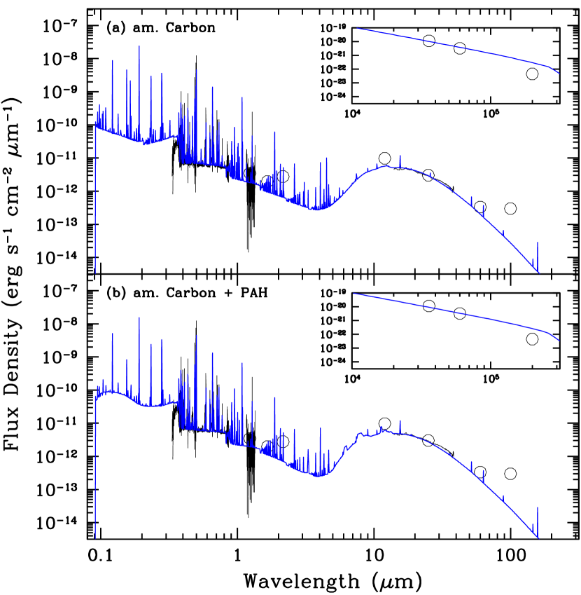
Figure 5.— The predicted SED from the P-I modeling (blue lines) by Cloudy. The observed data are indicated by the black lines or circles. In the inner small boxes we plot the radio data and the predicted SED. (upper panel) The predicted SED by Cloudy considering amorphous carbon only. (lower panel) The predicted SED considering amorphous carbon and PAH grains (see text).

Table 11The predicted relative line fluxes by the Cloudy models.

Ion	$\lambda$	$I$($\lambda$)obs	$I$($\lambda$)cloudy	$I$($\lambda$)cloudy	Walsh et al.
	(Å/$\mu$m)		Model A	Model B	(1997)
$[$O ii$]$	3727	9.25	27.80	25.60	10.86
$[$Ne iii$]$	3869	53.57	61.64	56.87	57.70
$[$S ii$]$	4068	2.07	2.95	3.12	2.78
$[$S ii$]$	4076	0.81	0.95	1.00	0.98
C ii	4267	1.10	1.19	1.31	0.97
O ii	4294	0.04	0.02	0.03	$\cdots$
$[$O iii$]$	4363	13.90	12.37	10.84	14.31
He i	4471	5.91	6.99	6.53	6.11
$[$Ar iv$]$	4740	0.73	0.99	0.82	0.74
$[$O iii$]$	4931	0.15	0.11	0.11	$\cdots$
$[$O iii$]$	4959	265.07	259.39	262.20	271.64
$[$O iii$]$	5007	792.07	780.77	789.22	790.83
$[$Ar iii$]$	5192	0.06	0.11	0.13	$\cdots$
$[$Fe iii$]$	5271	0.08	0.24	0.15	$\cdots$
$[$Cl iii$]$	5518	0.06	0.04	0.05	0.21
$[$Cl iii$]$	5538	0.16	0.15	0.17	0.13
$[$N ii$]$	5755	0.72	0.70	0.73	1.10
He i	5876	19.56	22.36	20.73	18.21
$[$S iii$]$	6312	1.63	1.06	1.14	2.47
$[$N ii$]$	6548	3.59	3.59	3.80	3.54
$[$N ii$]$	6583	10.92	10.61	11.22	11.43
He i	6678	4.92	5.20	4.88	4.77
$[$S ii$]$	6716	0.49	0.69	0.66	0.49
$[$S ii$]$	6731	1.10	1.42	1.41	1.10
$[$Ar iii$]$	7135	7.66	8.03	11.16	6.48
$[$Ar iv$]$	7171	0.04	0.04	0.03	$\cdots$
$[$Ar iv$]$	7263	0.04	0.03	0.02	$\cdots$
$[$O ii$]$	7323	8.29	16.84	15.74	6.24
$[$O ii$]$	7332	6.75	13.59	12.69	7.03
$[$Ar iii$]$	7751	1.84	1.94	2.69	1.22
$[$Cl iv$]$	8047	0.17	0.21	0.25	$\cdots$
C iii	8197	0.05	0.13	0.10	$\cdots$
He i	1.28	1.13	0.98	0.93	$\cdots$
H i	1.28	16.18	15.63	15.61	$\cdots$
$[$Ne iii$]$	15.55	31.41	29.87	30.92	$\cdots$
2MASS $J$	1.24	51.90	49.06	50.57	$\cdots$
2MASS $H$	1.66	40.00	27.37	32.20	$\cdots$
2MASS $Ks$	2.16	98.50	22.21	23.81	$\cdots$
IRS B	20.0	2182.05	2199.71	2044.33	$\cdots$
IRS C	30.0	1004.30	979.57	922.92	$\cdots$

Table 12The derived properties of the PN central star, ionized nebula, and dust by the P-I model.

Central star
parameters	Model A	Model B
$\log,L_{\star}/L_{\odot}$	3.60	3.57
$\log,T_{eff}$ (K)	5.07	4.93
$\log\,g$ (cm2 s-1)	6.0	6.0
composition	$[X,Y]$=0, $[Z]=-1$	$[X,Y]$=0, $[Z]=-1$
Nebula
parameters	Model A	Model B
composition	He:11.15,C:9.17,N:6.93,	He:11.08,C:9.19,N:7.03,
	O:8.29,Ne:7.43,S:6.15,	O:8.33,Ne:7.45,S:6.25,
	Cl:4.33,Ar:5.74,Fe:5.72	Cl:4.43,Ar:5.89,Fe:5.57
	others:[X/H]=–0.6	others:[X/H]=–0.6
geometry	spherical	spherical
$R_{\rm in}$/$R_{\rm out}$ (′′)	0.19/0.29	0.18/0.26
$\log,N_{\rm H}(R_{\rm in})$ (cm-3)	4.75	4.78
$\log F$(H$\beta$)	–12.02	–12.02
$M_{\rm gas}$ ($M_{\odot}$)	0.05	0.07
dust comp.	am. C	am. C + PAHs
$T_{\rm dust}$ (K)	100–150	100–200
$M_{\rm dust}$ ($M_{\odot}$)	2.9(–4)	4.0(–4)
$M_{\rm dust}$/$M_{\rm gas}$	5.92(–3)	5.58(–3)

Table 13Gas and grain carbon mass in Hen2-436.

parameters	Model A	Model B
gas C ($M_{\odot}$)	1.3(–3)	8.6(–4)
grain C ($M_{\odot}$)	2.9(–4)	4.0(–4)
gas + grain C ($M_{\odot}$)	1.6(–3)	1.3(–3)
$N$(gas + grain C)/$N$(H)†	1.8(–3)	2.3(–3)

In Table 12, we list the derived parameters of the PN central star, ionized gas nebula, and dust. In Figure 5 we present the predicted SED from Cloudy (blue lines). The upper and lower panels are the results of models A and B, respectively. In the inner small boxes we plot the radio flux densities (circles) from Dudziak et al. (2000) and the predicted SED. Dudziak et al. (2000) measured flux densities of 0.62/3.90/4.90 mJy at 1.46, 4.89, 8.40 GHz respectively. Although the predicted SED well matches the data in optical to radio wavelengths, it cannot explain the $\sim$30 $\mu$m bump and the $IRAS$ 100 $\mu$m data. The 30 $\mu$m bump might be from Magnesium Sulfide (MgS) grains, which are sometimes observed in C-rich PNe. At the present, since there are no available optical constants of MgS at UV wavelengths, we did not consider MgS in the SED models. Most of the IRAS 100 $\mu$m flux would be from the surrounding cold ISM because the spatial resolving power is $\sim$2^′ at this band. Accordingly, our models failed to explain the flux in these bands.

For Hen2-436, this work is the first successful estimate of the dust mass of 2.9(–4) $M_{\odot}$ in model A and 4.0(–4) $M_{\odot}$ in model B and temperatures of 100-150 K in model A and 100–200 K in model B. The derived dust-to-gas mass ratios in both models are slightly larger than the typical value in PNe having nebular radius of 10¹⁷ cm ($\sim$10^-3; Pottasch 1984). The value is rather close to the LMC ISM (4$\times$10^-3; Meixner et al. 2010). Lagadec et al. (2009, 2010) assumed a dust-to-gas mass ratio of 5$\times$10^-3 in radiative transfer modelings of C-rich stars in the Sgr dwarf galaxy.

We feel that model B can better explain the physical conditions of gas and dust in Hen2-436, because the line fluxes predicted by model B give a better fit to the observations and $T_{\rm eff}$ is not so high as to produce strong emission from He ii, which would originate in the stellar wind of Hen2-436. The predicted $T_{\rm eff}$ and $L_{\ast}$ are comparable to the values by Dudziak et al. (2000). At this time, there is no UV data of Hen2-436. The flux density profile in the UV region and the mid IR flux profile depend upon the central star temperature and luminosity as well as the dust composition. The predicted SEDs in the optical or longer wavelength regions by Models A and B do not show large differences, however a slight difference is found around 0.1–0.2 $\mu$m as can be seen in Figure 5. This discrepancy could be due to dust composition. Certainly in PNe, the bulk of the heating of the grains will be done by UV photons around 0.1 $\mu$m, where the dust absorption coefficient peaks. To further enlarge our understanding, UV and also 3–10 $\mu$m spectra would be necessary. These data would enable us to estimate the C abundance using C [iii] $\lambda\lambda$1906/09 lines and the CEL C/O ratio and also check for the existence of PAHs.

In general, the elemental abundances of PNe have been estimated based on gas emission lines only. Here, we can estimate gas and grain C mass through SED modeling. We can then investigate how much the C abundance increase if we include the contribution of grains. In Table 13, we present the gas and grain phase C mass in both models. It is remarkable that in model B, which is the best model at the present, $\sim$50 $\%$ of the gas C mass exists as grains. If the C abundance is measured using the sum of gas and grain C masses, the C abundance ($\log_{10}N$(C)/$N$(H)+12) would be 9.36 dex, which is $\sim$0.17 dex larger than the case of only gas C (9.19 in the case of gas C only, see Table 12). The grain C abundance might be considerable in PNe.

4.2. Evolutionary Status

In Figure 6 we plot the location of Hen2-436 and two Sgr dwarf galaxy PNe StWr2-21 and Wray16-423 (Zijlstra et al. 2006) and the post-AGB He-burning evolutionary tracks with $Z$ = 0.008 by Vassiliadis & Wood (1994). Since all these three Sgr dwarf galaxy PN have WR type central stars (Zijlstra et al. 2006), we assume that the central stars are hydrogen-poor. For Hen2-436, we find that $L_{\ast}$ predicted by models A and B has and uncertainty of $\sim$1200 $L_{\odot}$, which is estimated from the H$\beta$ flux and distance determination errors. The uncertainty of $T_{\rm eff}$ is $\sim$10 000 K. These evolutionary tracks suggest that the progenitors are 1.5–2 $M_{\odot}$ stars, which end their lives as white dwarfs with a core mass of $\sim$0.63–0.67 $M_{\odot}$. Among the above three PNe, Hen2-436 seems to be the youngest PN. The age of Hen2-436 is estimated from the evolutionary tracks to be $\sim$3000 yr after leaving the AGB phase. Gesicki & Zijlstra (2000) estimated the expansion velocity to be 14 km s^-1. When adopting the value $R_{out}$ = 0.26^′′ (see Table 12) and the distance of 24.8 kpc, the dynamical age is estimated to be $\sim$2200 yr, which is consistent with the evolutionary age.

4.3. Dust Mass-Loss Rate

If most of the observed dust is formed during the last two thermal pulses ($\sim$10 000 yr, Vassiliadis & Wood 1993 for the case of a 2.0 $M_{\odot}$ initial mass and $Z$ = 0.008), the dust mass-loss rate ($\dot{M}_{\rm dust}$) is estimated to be $<$3.1(–8) $M_{\odot}$ yr^-1. Lagadec et al. (2010) estimated a $\dot{M}_{\rm dust}$ of 0.97–2.52(–8) $M_{\odot}$ yr^-1 for IRAS18436-2849 in the Sgr dwarf galaxy. IRAS18436-2849 shows similar metallicity and luminosity to Hen2-436. For a C-rich metal-poor star ([Fe/H]$\sim$–1) IRAS12560+1656 in the Sgr dwarf galaxy stream, Groenewegen et al. (1997) estimated $\dot{M}_{\rm dust}$ to be 1.9(–9) $M_{\odot}$ yr^-1. Our estimated value is comparable to their values. Adopting a dust-to-gas mass ratio of 5.58(–3), the mass-loss rate $\dot{M}$ during the last two thermal pulses is estimated to be $<$5.5(–6) $M_{\odot}$ yr^-1, which is very close to the predicted mass-loss rate during the last two thermal pulses (Vassiliadis & Wood 1993 for the same case above).

Figure 6.— The evolutionary tracks for He-burning stars with $Z$ = 0.008 and the positions of three Sgr dwarf galaxy PNe.

Table 14The observed chemical abundances and the theoretical model.

Nebula	He	C	N	O	F	Ne	P	S	Ref
Hen2-436	11.09	9.08	7.38	8.35	5.69	7.62	5.72	6.83	(1)
StWr2-21	11.00	9.00	7.88	8.53	$\cdots$	7.54	$\cdots$	6.93	(2)
Wray16-423	11.03	8.86	7.68	8.33	$\cdots$	7.55	$\cdots$	6.67	(2)
Model
2.25 $M_{\odot}$ ($Z=0.008$)	11.01	9.07	8.00	8.54	5.00	7.95	5.18	6.85	(3)

4.4. Comparison between the Observed Chemical Abundances and the Theoretical Model

In Table 14, we present the observed elemental abundances of Hen2-436, StWr2-21, and Wray16-423 (Zijlstra et al. 2006) and predicted values from the theoretical models of Karakas (2010) for 2.25 $M_{\odot}$ stars with initial $Z$=0.008. The abundances of Sgr dwarf galaxy PNe are measured using gas emission lines only and their C abundances are derived from the ORL C lines. abundances from the models are the values at the end of the AGB. Karakas (2010) predicted that such stars end as white dwarfs with a core mass of 0.652 $M_{\odot}$, which is comparable to the core mass of Hen2-436 estimated from the evolutionary tracks. In the model for 2.25 $M_{\odot}$ stars with $Z$=0.008, a partial mixing zone, which produces a ¹³C pocket during the interpulse period and releases free neutrons, is not included and the mass-loss law during the AGB phase by Vassiliadis & Wood (1993) is adopted. For the models with $Z$=0.008, Karakas (2010) adopted LMC compositions from Russell & Dopita (1992). The accuracy of the predicted abundances by the models is on the order of 0.3 dex (A. Karakas in private communication). For the observed N and O abundances of Hen2-436, we adopted the values derived from the CELs.

In general the observed chemical abundances of the above three PNe agree well with the model of Karakas (2010) within estimation errors, which suggest that all three of these PNe have evolved from $\approx$2.25 $M_{\odot}$ single stars with initial LMC chemical compositions. The three Sgr dwarf galaxy PNe would have experienced evolution similar to LMC PNe, which is a remarkable finding. Some of the ¹⁴N in Hen2-436 might have been converted into ²²Ne by the double $\alpha$ particle capture process. The overabundances of ¹⁹F and ³¹P in Hen2-436 imply that an extensive partial mixing zone was formed and the extra neutrons were released in the He-rich intershell.

5. Conclusion

We estimated elemental abundances in the Sgr dwarf galaxy PN Hen2-436 based on the archived ESO/VLT FORS2 and $Spitzer$/IRS spectra. We detected candidates of [F ii]$\lambda$4790, [Kr iii]$\lambda$6826, and [P ii]$\lambda$7875 for the first time, which indicates that these elements are largely enhanced. We found a co-relation between C and F, P, and Kr abundances among PNe and C-rich stars. The detections of F, P and Kr in Hen2-436 support that F, P, and Kr together with C are certainly synthesized in the same layer and brought to the stellar surface by the third dredge-up. We detected some N ii and O ii ORLs and derived the ionic abundances from these lines. The discrepancy between O ORL and CEL abundances is $>$1 dex. We constructed a SED model considering dust and estimated the initial mass of the progenitor to be $\sim$1.5-2.0 $M_{\odot}$ with $Z$=0.008 and the age to be $\sim$3000 yr after the AGB phase. Hen2-436 shares its evolutionary status with the Sgr dwarf galaxy PNe StWr2-21 and Wray16-423. The observed elemental abundances of the three Sgr dwarf galaxy PNe could be explained by a theoretical nucleosynthesis model with initial mass 2.25 $M_{\odot}$, $Z$=0.008, and LMC chemical abundances. The SED model predicted that $>$2.9(–4) $M_{\odot}$ of carbon dust co-exists in the ionized nebula. Hen2-436 seems to have experienced evolution similar to LMC PNe. Based on the assumption that most of the observed dust is formed during the last two thermal pulses and the dust-to-gas mass ratio is 5.58(–3), the dust mass-loss rate and the total mass-loss rate are $<$3.1(–8) $M_{\odot}$ yr^-1 and $<$5.5(–6) $M_{\odot}$ yr^-1, respectively. Our estimated dust mass-loss rate is comparable to a similar metallicity and luminosity Sgr dwarf galaxy AGB star.

References

- (1) Abia, C., et al. 2010, ApJ, 715, L94
- (2) Acker, A., & Neiner, C. 2003, A&A, 403, 659
- (3) Appenzeller, I., et al. 1998, The Messenger, 94, 1
- (4) Baker, J. G., & Menzel, D. H. 1938, ApJ, 88, 52
- (5) Benjamin, R. A., Skillman, E. D., & Smits, D. P. 1999, ApJ, 514, 307
- (6) Bernard-Salas, J., Peeters, E., Sloan, G. C., Gutenkunst, S., Matsuura, M., Tielens, A. G. G. M., Zijlstra, A. A., & Houck, J. R. 2009, ApJ, 699, 1541
- (7) Biémont, E., & Hansen, J. E. 1986, Phys. Scr, 34, 116
- (8) Bregman, J. D., Allamandola, L. J., Witteborn, F. C., Tielens, A. G. G. M., & Geballe, T. R., 1989, ApJ, 344, 791
- (9) Busso, M., Gallino, R., & Wasserburg, G. J. 1999, ARA&A, 37, 239
- (10) Cahn, J. H., Kaler, J. B., & Stanghellini, L. 1992, A&AS, 94, 399
- (11) Cardelli, J. A., Clayton, G. C., & Mathis, J. S. 1989, ApJ, 345, 245
- (12) Cohen, M., & Barlow, M. J. 2005, MNRAS, 362, 1199
- (13) De Marco, O., & Barlow, M. J. 2001, Ap&SS, 275, 53
- (14) Desert, F.-X., Boulanger, F., & Puget, J.L. 1990, A&A, 237, 215
- (15) Dudziak, G., Péquignot, D., Zijlstra, A. A., & Walsh, J. R. 2000, A&A, 363, 717
- (16) Ferland, G. J. 2004, Bulletin of the American Astronomical Society, 36, 1574
- (17) Geballe, T. R., 1989, ApJ, 344, 791
- (18) Gesicki, K., & Zijlstra, A. A. 2000, A&A, 358, 1058
- (19) Girard, P., Köppen, J., & Acker, A. 2007, A&A, 463, 265
- (20) Groenewegen, M. A. T., Oudmaijer, R. D., & Ludwig, H.-G. 1997, MNRAS, 292, 686
- (21) Herwig, F. 2005, ARA&A, 43, 435
- (22) Houck, J. R., et al. 2004, SPIE, 5487, 62
- (23) Hyung, S., Aller, L. H., Feibelman, W. A., & Lee, S.-J. 2001, ApJ, 563, 889
- (24) Hyung, S., & Aller, L. H. 1997, MNRAS, 292, 71
- (25) Hyung, S., Aller, L. H., & Feibelman, W. A. 1994, MNRAS, 269, 975
- (26) Karakas, A. I. 2010, MNRAS, 403, 1413
- (27) Karakas, A. I., van Raai, M. A., Lugaro, M., Sterling, N. C., & Dinerstein, H. L. 2009, ApJ, 690, 1130
- (28) Karakas, A., & Lattanzio, J. C. 2007, PASA, 24, 103
- (29) Kingdon, J., & Ferland, G. J. 1995, ApJ, 442, 714
- (30) Kniazev, A. Y., et al. 2008, MNRAS, 388, 1667
- (31) Kunder, A., & Chaboyer, B. 2009, AJ, 137, 4478
- (32) Lagadec, E., Zijlstra, A. A., Mauron, N., Fuller, G., Josselin, E., Sloan, G. C., & Riggs, A. J. E. 2010, MNRAS, 403, 1331
- (33) Lagadec, E., et al. 2009, MNRAS, 396, 598
- (34) Liu, X.-W., Luo, S.-G., Barlow, M. J., Danziger, I. J., & Storey, P. J. 2001, MNRAS, 327, 141
- (35) Liu, X.-W., Storey, P. J., Barlow, M. J., & Clegg, R. E. S. 1995, MNRAS, 272, 369
- (36) Liu, X.-W., Storey, P. J., Barlow, M. J., Danziger, I. J., Cohen, M., & Bryce, M. 2000, MNRAS, 312, 585
- (37) Liu, Y., Liu, X.-W., Barlow, M. J., & Luo, S.-G. 2004, MNRAS, 353, 1251
- (38) Lugaro, M., Ugalde, C., Karakas, A. I., Görres, J., Wiescher, M., Lattanzio, J. C., & Cannon, R. C. 2004, ApJ, 615, 934
- (39) Lodders, K. 2003, ApJ, 591, 1220
- (40) Marcolino, W. L. F., Hillier, D. J., de Araujo, F. X., & Pereira, C. B. 2007, ApJ, 654, 1068
- (41) Mathis, J. S., Rumpl, W., & Nordsieck, K. H. 1977, ApJ, 217, 425
- (42) McLeod, B. A., Fabricant, D., Geary, J., Martini, P., Nystrom, G., Elston, R., Eikenberry, S. S., & Epps, H. 2004, Proc. SPIE, 5492, 1306
- (43) Meixner, M., et al. 2010, A&A, 518, L71
- (44) Mendoza, C., & Zeippen, C. J. 1982, MNRAS, 199, 1025
- (45) Otsuka, M., Tajitsu, A., Hyung, S., & Izumiura, H. 2010, ApJ, 723, 658
- (46) Otsuka, M., Izumiura, H., Tajitsu, A., & Hyung, S. 2008, ApJ, 682, L105
- (47) Pottasch, S. R., Bernard-Salas, J., & Roellig, T. L. 2009, A&A, 499, 249
- (48) Pottasch, S. R., Bernard-Salas, J., & Roellig, T. L. 2008, A&A, 481, 393
- (49) Pottasch, S. R., Bernard-Salas, J., Beintema, D. A., & Feibelman, W. A. 2003, A&A, 409, 599
- (50) Pottasch, S. R. 1984, “Planetary Nebulae”, Astrophysics and Space Science Library, 107
- (51) Rouleau, F., & Martin, P.G. 1991, ApJ, 377, 526
- (52) Ramos-Larios, G., Phillips, J. P., & Cuesta, L. C. 2010, MNRAS, 1733
- (53) Rudy, R. J., Rossano, G. S., Erwin, P., & Puetter, R. C. 1991, ApJ, 368, 468
- (54) Russell, S. C., & Dopita, M. A. 1992, ApJ, 384, 508
- (55) Schlegel, D. J., Finkbeiner, D. P., & Davis, M. 1998, ApJ, 500, 525
- (56) Schutte, W. A., Tielens, A.G.G.M., & Allamandolla, L.J., 1993, ApJ, 415, 397
- (57) Seaton, M. J. 1979, MNRAS, 187, 73P
- (58) Schoning, T. 1997, A&AS, 122, 277
- (59) Sterling, N. C., et al. 2009, Publications of the Astronomical Society of Australia, 26, 339
- (60) Sterling, N. C., & Dinerstein, H. L. 2008, ApJS, 174, 158
- (61) Storey, P. J., & Hummer, D. G. 1995, MNRAS, 272, 41
- (62) Surendiranath, R., & Pottasch, S. R. 2008, A&A, 483, 519
- (63) Tayal, S. S. 2004, ApJS, 150, 465
- (64) Tsamis, Y. G., Barlow, M. J., Liu, X.-W., Storey, P. J., & Danziger, I. J. 2004, MNRAS, 353, 953
- (65) Vassiliadis, E., & Wood, P. R. 1993, ApJ, 413, 641
- (66) Vassiliadis, E., & Wood, P. R. 1994, ApJS, 92, 125
- (67) Walsh, J. R., Dudziak, G., Minniti, D., & Zijlstra, A. A. 1997, ApJ, 487, 651
- (68) Wang, W., & Liu, X.-W. 2007, MNRAS, 381, 669
- (69) Wiese, W. L., Fuhr, J. R., & Deters, T. M. 1996, J.Phys.Chem.Ref.Data,Monograph No.7, “Atomic Transition Probabilities of Carbon, Nitrogen and Oxygen”, American Chemical Society, Washington,DC, and American Institute of Physics, New York
- (70) Wesson, R., Liu, X.-W., & Barlow, M. J. 2005, MNRAS, 362, 424
- (71) Wesson, R., Liu, X.-W., & Barlow, M. J. 2003, MNRAS, 340, 253
- (72) Werner, K., & Herwig, F. 2006, PASP, 118, 183
- (73) Zhang, Y., & Liu, X.-W. 2005, ApJ, 631, L61
- (74) Zijlstra, A. A., Gesicki, K., Walsh, J. R., Péquignot, D., van Hoof, P. A. M., & Minniti, D. 2006, MNRAS, 369, 875