Influence of fast interstellar gas flow on the dynamics of dust grains

Abstract

The orbital evolution of a dust particle under the action of a fast interstellar gas flow is investigated. The secular time derivatives of Keplerian orbital elements and the radial, transversal, and normal components of the gas flow velocity vector at the pericentre of the particle’s orbit are derived. The secular time derivatives of the semi-major axis, eccentricity, and of the radial, transversal, and normal components of the gas flow velocity vector at the pericentre of the particle’s orbit constitute a system of equations that determines the evolution of the particle’s orbit in space with respect to the gas flow velocity vector. This system of differential equations can be easily solved analytically. From the solution of the system we found the evolution of the Keplerian orbital elements in the special case when the orbital elements are determined with respect to a plane perpendicular to the gas flow velocity vector. Transformation of the Keplerian orbital elements determined for this special case into orbital elements determined with respect to an arbitrary oriented plane is presented. The orbital elements of the dust particle change periodically with a constant oscillation period or remain constant. Planar, perpendicular and stationary solutions are discussed.

The applicability of this solution in the Solar system is also investigated. We consider icy particles with radii from 1 to 10 $\mu$m. The presented solution is valid for these particles in orbits with semi-major axes from 200 to 3000 AU and eccentricities smaller than 0.8, approximately. The oscillation periods for these orbits range from 10⁵ to 2 $\times$ 10⁶ years, approximately.

1 Introduction

Since Poynting (1903) and Robertson (1937), the dynamics of dust grains has been investigated in many papers and its analysis is an inseparable part of astrophysics. The influence of the electromagnetic radiation of a central star is usually taken into account in the form of the Poynting-Robertson (P-R) effect (Poynting 1903; Robertson 1937; Wyatt and Whipple 1950; Burns et al. 1979; Klačka 2008). Beside the P-R effect, the stellar wind (corpuscular radiation of the star) can also affect the motion of dust particles. Covariant derivation of the acceleration caused by the stellar wind and its effects on the dynamics of dust grains were presented in Klačka et al. (2009b). The Solar magnetic field can affect the motion of charged dust particles in the Solar system (Parker 1958; Kimura and Mann 1998). Planets can capture the dust particles into the mean-motion resonances (Dermott et al. 1994; Reach et al. 1995). Because of the relative motion of the Sun with respect to the local interstellar medium, atoms of the interstellar medium approach the Sun. The direction of the approach is given by the actual velocity of the Sun with respect to the local interstellar medium. These approaching atoms form an interstellar gas flow. This flow of interstellar atoms through the Solar system has been already investigated in the past (e.g. Fahr 1996; Möbius et al. 2009; Alouani-Bibi et al. 2011). This interstellar gas flow can affect the dynamics of dust grains in outer parts of the Solar system. The assumption that dust particles in orbits around other stars can be also affected by interstellar gas flow is supported by the recent detection of debris disks around stars with asymmetric morphology caused by a fast motion of the disk through a cloud of interstellar matter (Hines et al. 2007; Debes et al. 2009).

The influence of interstellar gas flow on the dynamics of a spherical dust particle was investigated by Scherer (2000), who calculated the secular time derivatives of the particle’s angular momentum and the Laplace-Runge-Lenz vector caused by the interstellar gas flow. He has come to the conclusion that the particle’s semi-major axis can increase exponentially (Scherer 2000, p. 334). This result contradicts results of Pástor et al. (2011). Here the secular time derivatives of the Keplerian orbital elements of the dust particle under the action of a fast interstellar gas flow were for the first time calculated for arbitrary orientations of the orbit. Pástor et al. (2011) states that the secular semi-major axis of the dust particle must decrease under the action of the interstellar gas flow. The rate of decrease is proportional to the semi-major axis. Decrease of the semi-major axis only happens in secular time-scales. Therefore, the exact calculation of the secular time derivative of the semi-major axis was necessary. This result was confirmed also by Belyaev and Rafikov (2010) who investigated the motion of a dust particle in the outer region of the Solar system behind the solar wind termination shock. They calculated the orbital evolution of the dust particle under the action of a constant mono-directional force, i.e., they solved a case of the classical Stark problem (for more information about the Stark problem see Lantoine and Russell 2011 and the references therein). In the Stark problem it is assumed that the orbital speed of the dust grain with respect to a central object can be neglected in comparison with the speed of the interstellar gas flow. The relative velocity terms are in Pástor et al. (2011) taken into account to the first order of accuracy in the calculation of the secular time derivatives of Keplerian orbital elements. Belyaev and Rafikov (2010) reproduced the result of Pástor et al. (2011) on the secular evolution of the semi-major axis of the particle’s orbit. However, the case of a mono-directional force (i.e., the Stark problem) can be important for those stars where the relative speed of the neutral gas with respect to the central star is high. Such a situation can occur, for example, in merging galaxies when a star from the first galaxy moves through a molecular cloud of the second galaxy.

Belyaev and Rafikov (2010) used the orbit-averaged Hamiltonian method. In this paper we use a method based on orbit-averaged time derivatives of Keplerian orbital elements. Using this different method we confirm results of Belyaev and Rafikov (2010). We not only use a new method, we also find new results. We find an explicit form for the time dependence of all Keplerian orbital elements determined with respect to a reference plane perpendicular to the gas flow velocity vector. Mainly the time dependence of the longitude of the ascending node will represent a generalization of Belyaev and Rafikov (2010) results. We find a transformation for the orbital elements determined with respect to the reference plane perpendicular to the gas flow velocity vector into an arbitrarily oriented reference plane. We determine the maximal and minimal values of eccentricity for numerous special cases. We study in detail the behaviour of the solution for the planar case and for the case when the gas flow velocity vector is perpendicular to the line of apsides. Properties of the solution in the Solar system are discussed.

2 Equation of motion

In order to find the acceleration of a spherical dust particle caused by an interstellar gas flow we will assume (a) that the dimensions of the dust particle are small in comparison with the mean free path of the interstellar gas atoms, (b) that the mass of the dust particle is large in comparison with the mass of the interstellar gas atoms, and (c) that the molecules are specularly or diffusely reflected from the surface of the dust particle. These assumptions lead to the following acceleration (Baines et al. 1965)

$$\frac{d\vec{v}}{dt}=-~{}c_{D}~{}\gamma_{H}~{}|\vec{v}-\vec{v}_{H}|~{}\left(\vec{v}-\vec{v}_{H}\right)~{},$$ (1)

where $\vec{v}$ is the velocity of the dust grain in the stationary frame, $\vec{v}_{H}$ is the constant velocity vector of atoms in the flow in the stationary frame, $c_{D}$ is the drag coefficient, and $\gamma_{H}$ is the collision parameter. For the collision parameter we can write

$$\gamma_{H}=n_{H}~{}\frac{m_{H}}{m}~{}A~{},$$ (2)

where $m_{H}$ is the mass of the neutral hydrogen atom, $n_{H}$ is the concentration of the interstellar neutral hydrogen atoms, and $A$ $=$ $\pi{R}^{2}$ is the geometrical cross section of a spherical dust grain of radius $R$ and mass $m$. Assumption (a) is a reasonable approximation to conditions in interstellar space. Therefore, Eq. (1) is valid for all dust particles with dimensions for which assumption (b) holds.

In order to find the final equation of motion we further assume (d) that the dust particle orbits around a star. Therefore we take into account also the electromagnetic radiation of the star in the form of the P-R effect. The equation of motion then has the form

$$\frac{d\vec{v}}{dt} = -~{}\frac{\mu}{r^{2}}~{}\vec{e}_{R}$$ (3)

$$+~{}\beta~{}\frac{\mu}{r^{2}}\left[\left(1-\frac{\vec{v}\cdot\vec{e}_{R}}{c}\right)\vec{e}_{R}-\frac{\vec{v}}{c}\right]$$

$$-~{}c_{D}~{}\gamma_{H}~{}|\vec{v}-\vec{v}_{H}|~{}\left(\vec{v}-\vec{v}_{H}\right)~{}.$$

where $\mu$ $=$ $GM$, $G$ is the gravitational constant, $M$ is the mass of the star, $\vec{r}$ is the position vector of the particle with respect to the star, $r$ $=$ $|\vec{r}|$, $\vec{e}_{R}$ $=$ $\vec{r}/r$, and $c$ is the speed of light in vacuum. Parameter $\beta$ is defined as the ratio of the electromagnetic radiation pressure force and the gravitational force between the star and the particle at rest with respect to the star

$$\beta=\frac{3~{}L~{}\bar{Q}^{\prime}_{pr}}{16~{}\pi~{}c~{}\mu~{}R~{}\varrho}~{}.$$ (4)

Here, $L$ is the star luminosity, $\bar{Q}^{\prime}_{pr}$ is the dimensionless efficiency factor for radiation pressure integrated over the star spectrum and calculated for the radial direction ($\bar{Q}^{\prime}_{pr}$ $=$ 1 for a perfectly absorbing sphere), and $\varrho$ is the mass density of the particle. The second term represents the P-R effect neglecting terms of higher orders in $\vec{v}/c$ than the first (Klačka 2008). Eq. 3 was used in numerical experiments by Marzari and Thébault (2011).

We also restrict the possible speeds of the interstellar gas flow. We will assume (e) that the speed of the interstellar gas flow is much greater that the mean thermal speed of the gas in the flow. For interstellar gas flow speeds $v_{H}$ $=$ $|\vec{v}_{H}|$ comparable to the mean thermal speed of the gas $c_{D}$ is a function of $v_{H}$ (Baines et al. 1965). However, $c_{D}$ has an approximately constant value for those interstellar gas flow speeds much greater that the mean thermal speed of the gas (Baines et al. 1965; Banaszkiewicz et al. 1994; Scherer 2000; Klačka et al. 2009a).

We also assume (f) that the speed of the interstellar gas flow is much greater than the speed of the dust grain in the stationary frame associated with the central star.

Finally, we assume (g) that the secular time derivatives of the semi-major axis and the eccentricity of the particle’s orbit caused by the P-R effect during orbital evolution are low in comparison with the values of the semi-major axis and the eccentricity, respectively. This assumption is reasonable for grains with large semi-major axes and small eccentricities (Wyatt and Whipple 1950). These particles have small orbital speeds. Therefore, in the P-R effect, the terms depending on velocity can be neglected in comparison with the Keplerian term.

Assumptions (a)–(g) lead to the final equation of motion

$$\frac{d\vec{v}}{dt} = -~{}\frac{\mu~{}(1-\beta)}{r^{2}}~{}\vec{e}_{R}+c_{D}~{}\gamma_{H}~{}v_{H}~{}\vec{v}_{H}$$ (5)

$$= -~{}\frac{\mu_{\beta}}{r^{2}}~{}\vec{e}_{R}+\alpha~{}\vec{v}_{H}~{}.$$

If the radial stellar wind is also considered in Eq. (3), then Eq. (5) remain unchanged (Klačka et al. 2009b). However, assumptions (f) and (g) require radial distances that are probably larger than the radial distance to the stellar wind termination shock for the majority of Sun-like stars.

3 Secular evolution of Keplerian orbital elements

We want to find the influence of the constant acceleration given by the second term in Eq. (5) on the secular evolution of a particle’s orbit. We will assume (h) that constant acceleration can be considered as a perturbation acceleration to the central acceleration caused by the gravity of the central star. For the applicability of the assumptions (f)–(h) in the Solar system we refer the reader to Appendix A. We denote the components of the hydrogen gas velocity vector in the stationary Cartesian frame associated with the central star as $\vec{v}_{H}$ $=$ $(v_{HX},v_{HY},v_{HZ})$. In order to compute the secular time derivatives of the Keplerian orbital elements ($a$, the semi-major axis; $e$, the eccentricity; $\omega$, the argument of the pericentre; $\Omega$, the longitude of the ascending node; $i$, the inclination) we want to use the Gauss perturbation equations of celestial mechanics. To do this, we need to know the radial, transversal, and normal components of acceleration given by the second term in Eq. (5). The orthogonal radial, transversal, and normal unit vectors of the particle on a Keplerian orbit are (e.g., Pástor 2009)

$$\vec{e}_{R} = \left(\cos\Omega~{}\cos(f+\omega)-\sin\Omega~{}\sin(f+\omega)~{}\cos i~{},\right.$$ (6)

$$\left.\sin\Omega~{}\cos(f+\omega)+\cos\Omega~{}\sin(f+\omega)~{}\cos i~{},\right.$$

$$\left.\sin(f+\omega)~{}\sin i\right)~{},$$

$$\vec{e}_{T} = \left(-\cos\Omega~{}\sin(f+\omega)-\sin\Omega~{}\cos(f+\omega)~{}\cos i~{},\right.$$ (7)

$$\left.-\sin\Omega~{}\sin(f+\omega)+\cos\Omega~{}\cos(f+\omega)~{}\cos i~{},\right.$$

$$\left.\cos(f+\omega)~{}\sin i\right)~{},$$

$$\vec{e}_{N} = (\sin\Omega~{}\sin i,~{}-\cos\Omega~{}\sin i,~{}\cos i)~{},$$ (8)

where $f$ is the true anomaly. For the radial, transversal and normal components of the perturbation acceleration, we obtain

$$a_{R} = \alpha~{}\vec{v}_{H}\cdot\vec{e}_{R}=\alpha~{}A~{},$$ (9)

$$a_{T} = \alpha~{}\vec{v}_{H}\cdot\vec{e}_{T}=\alpha~{}B~{},$$ (10)

$$a_{N} = \alpha~{}\vec{v}_{H}\cdot\vec{e}_{N}=\alpha~{}C~{}.$$ (11)

Now we can use the Gauss perturbation equations of celestial mechanics to compute the time derivatives of the orbital elements. The perturbation equations have the form (cf., e.g., Murray and Dermott 1999; Danby 1988)

$$\frac{da}{dt} = \frac{2~{}a}{1-e^{2}}~{}\sqrt{\frac{p}{\mu_{\beta}}}~{}\left[a_{R}~{}e~{}\sin f+a_{T}\left(1+e\cos f\right)\right]~{},$$

$$\frac{de}{dt} = \sqrt{\frac{p}{\mu_{\beta}}}~{}\left[a_{R}~{}\sin f+a_{T}\left(\cos f+\frac{e+\cos f}{1+e\cos f}\right)\right]~{},$$

$$\frac{d\omega}{dt} = -~{}\frac{1}{e}~{}\sqrt{\frac{p}{\mu_{\beta}}}~{}\left(a_{R}~{}\cos f-a_{T}~{}\frac{2+e\cos f}{1+e\cos f}~{}\sin f\right)$$

$$-~{}\frac{r}{\sqrt{\mu_{\beta}p}}~{}a_{N}~{}\frac{\sin(f+\omega)}{\sin i}~{}\cos i~{},$$

$$\frac{d\Omega}{dt} = \frac{r}{\sqrt{\mu_{\beta}p}}~{}a_{N}~{}\frac{\sin(f+\omega)}{\sin i}~{},$$

$$\frac{di}{dt} = \frac{r}{\sqrt{\mu_{\beta}p}}~{}a_{N}~{}\cos(f+\omega)~{},$$ (12)

where $p$ $=$ $a(1-e^{2})$. The time average of any quantity $g$ during one orbital period $T$ can be computed using

$$\left\langle g\right\rangle = \frac{1}{T}\int_{0}^{T}g~{}dt=\frac{\sqrt{\mu_{\beta}}}{2~{}\pi~{}a^{3/2}}\int_{0}^{2\pi}g\left(\frac{df}{dt}\right)^{-1}df$$ (13)

$$= \frac{\sqrt{\mu_{\beta}}}{2~{}\pi~{}a^{3/2}}\int_{0}^{2\pi}g\left(\frac{\sqrt{\mu_{\beta}p}}{r^{2}}\right)^{-1}df$$

$$= \frac{1}{2~{}\pi~{}a^{2}~{}\sqrt{1-e^{2}}}\int_{0}^{2\pi}g~{}r^{2}~{}df~{},$$

where the second ($\sqrt{\mu_{\beta}p}$ $=$ $r^{2}df/dt$) and the third ($4\pi^{2}a^{3}$ $=$ $\mu_{\beta}T^{2}$) of Kepler’s laws were used. From Eqs. (9)–(13) we finally obtain for the secular time derivatives of the Keplerian orbital elements

$$\left\langle\frac{da}{dt}\right\rangle = 0~{},$$ (14)

$$\left\langle\frac{de}{dt}\right\rangle = \frac{3~{}\alpha}{2}~{}\sqrt{\frac{p}{\mu_{\beta}}}~{}I~{},$$ (15)

$$\left\langle\frac{d\omega}{dt}\right\rangle = -~{}\frac{3~{}\alpha}{2}~{}\sqrt{\frac{p}{\mu_{\beta}}}~{}\left(\frac{S}{e}-C~{}\frac{\cos i}{\sin i}~{}\frac{e\sin\omega}{1-e^{2}}\right)~{},$$ (16)

$$\left\langle\frac{d\Omega}{dt}\right\rangle = -~{}\frac{3~{}\alpha}{2}~{}\sqrt{\frac{p}{\mu_{\beta}}}~{}\frac{C}{\sin i}~{}\frac{e~{}\sin\omega}{1-e^{2}}~{},$$ (17)

$$\left\langle\frac{di}{dt}\right\rangle = -~{}\frac{3~{}\alpha}{2}~{}\sqrt{\frac{p}{\mu_{\beta}}}~{}C~{}\frac{e~{}\cos\omega}{1-e^{2}}~{},$$ (18)

where the quantities

$$S = (\cos\Omega~{}\cos\omega-\sin\Omega~{}\sin\omega~{}\cos i)~{}v_{HX}$$

$$+~{}(\sin\Omega~{}\cos\omega+\cos\Omega~{}\sin\omega~{}\cos i)~{}v_{HY}$$

$$+~{}\sin\omega~{}\sin i~{}v_{HZ}~{},$$

$$I = (-\cos\Omega~{}\sin\omega-\sin\Omega~{}\cos\omega~{}\cos i)~{}v_{HX}$$

$$+~{}(-\sin\Omega~{}\sin\omega+\cos\Omega~{}\cos\omega~{}\cos i)~{}v_{HY}$$

$$+~{}\cos\omega~{}\sin i~{}v_{HZ}~{},$$

$$C = \sin\Omega~{}\sin i~{}v_{HX}-\cos\Omega~{}\sin i~{}v_{HY}+\cos i~{}v_{HZ}~{},$$ (19)

are values of $A$ $=$ $\vec{v}_{H}\cdot\vec{e}_{R}$, $B$ $=$ $\vec{v}_{H}\cdot\vec{e}_{T}$ and $C$ $=$ $\vec{v}_{H}\cdot\vec{e}_{N}$ at the pericentre of the particle orbit ($f$ $=$ 0), respectively. The value of $C$ is a constant on a given oscular orbit. The values of $S$, $I$ and $C$ are depicted in Fig. 1.

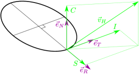
Figure 1: A schematic representation of the values $S$, $I$ and $C$ for a given orbit.

For the special case $\vec{v}_{H}$ $=$ $(-v_{H},0,0)$ the system of Eqs. (14)–(18) and Eqs. (3) reduces to the system of Eqs. (3)–(7) in Mignard and Henon (1984) with the exception of one term in the secular time derivative of the longitude of ascending node. Mignard and Henon (1984) studied the motion of a particle around a planet subject to radiation pressure from a central star. Mathematically, they considered the Stark problem in a rotating reference frame. The extra term in the secular time derivative of the longitude of ascending node is caused by the Coriolis force. The Stark problem is recovered if the rotation rate is set to zero. Because of the extra term caused by the Coriolis force their analytical solution is different and does not correspond to the solution which will be given in this paper. Their solution of the Stark problem is not easy to see from their notation in the rotating reference frame. Moreover, they considered only the case for which $\vec{v}_{H}$ lies in the plane with $i$ $=$ 0 and is antiparallel with $x$ axis. Our solution will be more general.

4 Secular evolution of orbit with respect to gas flow velocity vector

The parameters $S$, $I$ and $C$ determine the position of the orbit with respect to the gas flow velocity vector. Therefore, their time derivatives are useful for a description of the evolution of the orbit’s position in space. Putting Eqs. (16)–(18) into the formulas for the averaged time derivatives of the quantities $S$, $I$ and $C$ given by Eqs. (3), we obtain

$$\left\langle\frac{dS}{dt}\right\rangle = -~{}\frac{3~{}\alpha}{2}~{}\sqrt{\frac{p}{\mu_{\beta}}}~{}\frac{S~{}I}{e}~{},$$ (20)

$$\left\langle\frac{dI}{dt}\right\rangle = -~{}\frac{3~{}\alpha}{2}~{}\sqrt{\frac{p}{\mu_{\beta}}}~{}\left(\frac{eC^{2}}{1-e^{2}}-\frac{S^{2}}{e}\right)~{},$$ (21)

$$\left\langle\frac{dC}{dt}\right\rangle = \frac{3~{}\alpha}{2}~{}\sqrt{\frac{p}{\mu_{\beta}}}~{}\frac{e~{}I~{}C}{1-e^{2}}~{}.$$ (22)

Eqs. (20)–(22) are not independent, because $S$ $\langle dS/dt\rangle$ $+$ $I$ $\langle dI/dt\rangle$ $+$ $C$ $\langle dC/dt\rangle$ $=$ 0 always hold. Eqs. (20)–(22) together with Eqs. (14)–(15) represent the system of equations that determines the evolution of the particle’s orbit in space with respect to the gas flow velocity vector. All orbits that are created with rotations of one orbit around the line aligned with the gas flow velocity vector and going through the centre of gravity will undergo the same evolution determined by this system of equations.

Now we find the solution of the system of equations given by Eqs. (14)–(15) and Eqs. (20)–(22). If we combine Eq. (15) with Eq. (20), then we obtain

$$\left\langle\frac{dS}{dt}\right\rangle=-\left\langle\frac{de}{dt}\right\rangle\frac{S}{e}~{}.$$ (23)

This equation leads, for $S$ $\neq$ 0, to the differential equation

$$\frac{dS}{S}=-~{}\frac{de}{e}~{},$$ (24)

with the solution

$$|S|=\frac{D}{e}~{}.$$ (25)

Here, $D$ is a constant which can be determined from the initial conditions. Thus, if the major axis of the orbit is aligned with the direction of the gas flow velocity vector, then the eccentricity is minimal. If we combine Eq. (15) with Eq. (22), then we obtain

$$\left\langle\frac{dC}{dt}\right\rangle=\frac{e~{}C}{1-e^{2}}\left\langle\frac{de}{dt}\right\rangle~{}.$$ (26)

This equation leads, for $C$ $\neq$ 0, to the differential equation

$$\frac{dC}{C}=\frac{e~{}de}{1-e^{2}}~{},$$ (27)

with the solution

$$|C|=\frac{F}{\sqrt{1-e^{2}}}~{},$$ (28)

where $F$ is an integration constant. Thus, if the magnitude of the normal component of $\vec{v}_{H}$ measured in the perihelion is maximal, then the eccentricity is maximal. For $I$ we obtain from $S^{2}$ $+$ $I^{2}$ $+$ $C^{2}$ $=$ $v^{2}_{H}$

$$|I|=\sqrt{v^{2}_{H}-\frac{D^{2}}{e^{2}}-\frac{F^{2}}{1-e^{2}}}~{}.$$ (29)

If $S$ $=$ 0, then from Eq. (20) we obtain $\langle dS/dt\rangle$ $=$ 0. Since Eq. (28) holds for the case $S$ $=$ 0 and $C$ $\neq$ 0, also Eq. (29) with $D$ $=$ 0 holds. Therefore we put $D$ $=$ 0 in Eq. (25) for the case $S$ $=$ 0 and $C$ $\neq$ 0. If $C$ $=$ 0, then from Eq. (22) we obtain $\langle dC/dt\rangle$ $=$ 0. Since Eq. (25) holds for the case $C$ $=$ 0 and $S$ $\neq$ 0, also Eq. (29) with $F$ $=$ 0 holds. Therefore we put $F$ $=$ 0 in Eq. (28) for the case $C$ $=$ 0 and $S$ $\neq$ 0. If $S$ $=$ 0 and $C$ $=$ 0, then we have $|I|$ $=$ $v_{H}$. Therefore we put $D$ $=$ 0 and $F$ $=$ 0 in Eq. (25) and Eq. (28), respectively. We come to the conclusion that Eqs. (25), (28) and (29) always hold during the orbital motion of the particle. Eq. (25) and Eq. (28) together with the properties of the system of differential equations given by Eqs. (14)–(15) and Eqs. (20)–(22) imply that $S$ and $C$ can not change sign during the orbital evolution of the particle. If $D$ $\neq$ 0, then both $S$ and $e$ must be non-zero during the orbital evolution of the particle. Similarly, if $F$ $\neq$ 0, then $C$ $\neq$ 0 and $e$ $\neq$ 1 during the orbital evolution of the particle. For the special cases $D$ $=$ 0 or $F$ $=$ 0 is necessary to use the properties of the whole system the differential equations given by Eqs. (14)–(15) and Eqs. (20)–(22), because, as we will see later, in these cases the eccentricity can be close to 0 or 1, respectively. Therefore we can write

$$S=\frac{U}{e}~{},$$ (30)

$$C=\frac{V}{\sqrt{1-e^{2}}}$$ (31)

and

$$|I|=\sqrt{v^{2}_{H}-\frac{U^{2}}{e^{2}}-\frac{V^{2}}{1-e^{2}}}~{},$$ (32)

where $U$ and $V$ are some constants. We come to the conclusion that also Eqs. (30)–(32) always hold during the orbital motion of the particle.

The $S$, $|I|$, and $C$ components of the hydrogen gas velocity vector at the pericentre of the particle’s orbit depend only on the particle’s eccentricity. To find the evolution of the eccentricity, we insert Eq. (32) into Eq. (15). We obtain

$$\frac{de}{dt} = \pm~{}\frac{3~{}\alpha~{}v_{H}}{2~{}e}~{}\sqrt{\frac{a}{\mu_{\beta}}}~{}$$ (33)

$$\times~{}\sqrt{e^{2}(1-e^{2})-\frac{U^{2}}{v^{2}_{H}}~{}(1-e^{2})-\frac{V^{2}}{v^{2}_{H}}~{}e^{2}}~{}.$$

The plus sign is for positive values of $I$ and the minus sign for negative values of $I$. If $I$ is negative, then the eccentricity decreases. If $I$ is positive, then the eccentricity increases. In order to integrate this equation we rewrite the expression in the second square root in the following form

$$e^{2}(1-e^{2})-\frac{U^{2}}{v^{2}_{H}}~{}(1-e^{2})-\frac{V^{2}}{v^{2}_{H}}~{}e^{2}=(e^{2}_{1}-e^{2})(e^{2}-e^{2}_{2})~{},$$ (34)

where

$$e^{2}_{1}=\frac{1+\frac{U^{2}}{v^{2}_{H}}-\frac{V^{2}}{v^{2}_{H}}}{2}+\sqrt{\left(\frac{1+\frac{U^{2}}{v^{2}_{H}}-\frac{V^{2}}{v^{2}_{H}}}{2}\right)^{2}-\frac{U^{2}}{v^{2}_{H}}}~{},$$ (35)

$$e^{2}_{2}=\frac{1+\frac{U^{2}}{v^{2}_{H}}-\frac{V^{2}}{v^{2}_{H}}}{2}-\sqrt{\left(\frac{1+\frac{U^{2}}{v^{2}_{H}}-\frac{V^{2}}{v^{2}_{H}}}{2}\right)^{2}-\frac{U^{2}}{v^{2}_{H}}}~{}.$$ (36)

It is possible to show (using Eqs. 30, 31 and 32) that the expression in the square root is always positive or zero, $e^{2}_{1}$ $\in$ [0, 1] and $e^{2}_{2}$ $\in$ [0, 1]. From Eq. (33) we obtain for $I$ $\neq$ 0

$$\int\frac{e~{}de}{\sqrt{(e^{2}_{1}-e^{2})(e^{2}-e^{2}_{2})}} = \arcsin\sqrt{\frac{e^{2}-e^{2}_{2}}{e^{2}_{1}-e^{2}_{2}}}+\varphi$$ (37)

$$= \pm~{}\frac{3~{}\alpha~{}v_{H}}{2}~{}\sqrt{\frac{a}{\mu_{\beta}}}~{}t~{},$$

where $\varphi$ is an integration constant. Hence

$$e^{2}=\frac{e^{2}_{1}+e^{2}_{2}}{2}-\frac{e^{2}_{1}-e^{2}_{2}}{2}~{}\cos\left(\pm~{}3\alpha v_{H}~{}\sqrt{\frac{a}{\mu_{\beta}}}~{}t-2\varphi\right)~{}.$$ (38)

From this equation we can see that the eccentricity changes between its minimal value $e_{2}$ and its maximal value $e_{1}$ for one solution determined by the choice of the sign ($+$ or $-$). We denote the time close to the maximum eccentricity $e_{1}$ as $t_{M}$. From Eq. (38) we obtain for values of $\varphi$ at the time $t_{M}$

$$2\varphi_{+}=3~{}\alpha~{}v_{H}~{}\sqrt{\frac{a}{\mu_{\beta}}}~{}t_{M}-\pi-2~{}k_{1}~{}\pi~{},$$ (39)

$$2\varphi_{-}=-~{}3~{}\alpha~{}v_{H}~{}\sqrt{\frac{a}{\mu_{\beta}}}~{}t_{M}-\pi-2~{}k_{2}~{}\pi~{},$$ (40)

where $k_{1}$ and $k_{2}$ are two integers. In Eq. (38) both these values lead to the same solution

$$e^{2}=\frac{e^{2}_{1}+e^{2}_{2}}{2}+\frac{e^{2}_{1}-e^{2}_{2}}{2}~{}\cos\left(3\alpha v_{H}~{}\sqrt{\frac{a}{\mu_{\beta}}}~{}(t-t_{M})\right)~{}.$$ (41)

This solution is in accordance with the result of Belyaev and Rafikov (2010) up to the definition of an additive constant for the time. The eccentricity changes periodically with the oscillation period

$$T_{e}=\frac{2~{}\pi}{3~{}\alpha~{}v_{H}}~{}\sqrt{\frac{\mu_{\beta}}{a}}~{}.$$ (42)

For a connection between this result (obtained from Eq. 5) and the results obtained from the equation of motion with the relative velocity $\vec{v}$ included in the force caused by the interstellar gas flow, we refer the reader to Appendix B. The values of $T_{e}$ for dust particles in the Solar system are in Table 1. For the Solar system we used $L_{\odot}$ $=$ 3.842 $\times$ 10²⁶ W (Bahcall 2002), $c_{D}$ $=$ 2.6 (Banaszkiewicz et al. 1994; Scherer 2000; Pástor et al. 2011), $n_{H}$ $=$ 0.2 cm^-3 (Belyaev and Rafikov 2010) and $v_{H}$ $=$ 26 km s^-1 (e.g. Lallement 1996; Landgraf et al. 1999) (see Appendix A).

$R$ $=$ 1 $\mu$m	$R$ $=$ 2 $\mu$m	$R$ $=$ 5 $\mu$m	$R$ $=$ 10 $\mu$m
$a$ $T_{e}$ [AU] $\left[10^{5}\atop\mbox{years}\right]$ 200 2.06 300 1.68 400 1.46 500 1.30 600 1.19 700 1.10	$a$ $T_{e}$ [AU] $\left[10^{5}\atop\mbox{years}\right]$ 200 5.35 400 3.78 600 3.09 800 2.67 1000 2.39 1200 2.18	$a$ $T_{e}$ [AU] $\left[10^{5}\atop\mbox{years}\right]$ 200 14.90 600 8.60 1000 6.66 1400 5.63 1800 4.97 2200 4.49	$a$ $T_{e}$ [AU] $\left[10^{5}\atop\mbox{years}\right]$ 500 19.45 1000 13.75 1500 11.23 2000 9.73 2500 8.70 3000 7.94

Table 1: Oscillation periods $T_{e}$ determined for orbits with various semi-major axes in the Solar system. Dust particles with radius $R$ $\in$ {1 $\mu$m, 2 $\mu$m, 5 $\mu$m, 10 $\mu$m}, mass density $\varrho$ $=$ 1 g cm^-3 and $\bar{Q}^{\prime}_{pr}$ $=$ 1 are used.

To find the time evolution of $S$, $|I|$ and $C$, we can put Eq. (41) into Eqs. (30)–(32). $S$, $|I|$ and $C$ also change periodically with period $T_{e}$. Now we find the evolution of $I$ from Eq. (32). If we put Eq. (41) into Eq. (34), then we get

$$(e^{2}_{1}-e^{2})(e^{2}-e^{2}_{2}) = \left(\frac{e^{2}_{1}-e^{2}_{2}}{2}\right)^{2}$$ (43)

$$\times~{}\sin^{2}\left(3\alpha v_{H}~{}\sqrt{\frac{a}{\mu_{\beta}}}~{}(t-t_{M})\right)~{}.$$

Hence,

$$|I|=\frac{v_{H}}{e~{}\sqrt{1-e^{2}}}~{}\frac{e^{2}_{1}-e^{2}_{2}}{2}~{}\left|\sin\left(3\alpha v_{H}~{}\sqrt{\frac{a}{\mu_{\beta}}}~{}(t-t_{M})\right)\right|~{}.$$ (44)

If $I$ is negative, then the secular eccentricity must decrease (see Eq. 15). Therefore if we compare the evolutions given by Eq. (41) and Eq. (44), we come to the conclusion that

$$I=-~{}\frac{v_{H}}{e~{}\sqrt{1-e^{2}}}~{}\frac{e^{2}_{1}-e^{2}_{2}}{2}~{}\sin\left(3\alpha v_{H}~{}\sqrt{\frac{a}{\mu_{\beta}}}~{}(t-t_{M})\right)~{}.$$ (45)

Eq. (41) and Eq. (45) hold also for the special cases $U$ $=$ 0 or $V$ $=$ 0.

4.1 Planar case

$C$ $=$ 0 for the special case when the velocity of the hydrogen gas $\vec{v}_{H}$ lies in the orbital plane of the particle. Putting $C$ $=$ 0 ($V$ $=$ 0) in Eqs. (35)–(36), one gets

$$e^{2}_{1}=1~{},$$ (46)

$$e^{2}_{2}=\frac{U^{2}}{v^{2}_{H}}~{}.$$ (47)

Therefore the minimum eccentricity is $|U|/v_{H}$ and the maximum eccentricity is 1. Using Eqs. (46)–(47) we obtain from Eqs. (30), (41), and (45), for the planar case,

$$S=\frac{U}{e}~{},$$ (48)

$$I=-~{}\frac{v_{H}}{e~{}\sqrt{1-e^{2}}}~{}\frac{1-\frac{U^{2}}{v^{2}_{H}}}{2}~{}\sin\left(3\alpha v_{H}~{}\sqrt{\frac{a}{\mu_{\beta}}}~{}(t-t_{M})\right)~{},$$ (49)

$$e^{2}=1-\left(1-\frac{U^{2}}{v^{2}_{H}}\right)\sin^{2}\left(\frac{3\alpha v_{H}}{2}~{}\sqrt{\frac{a}{\mu_{\beta}}}~{}(t-t_{M})\right)~{}.$$ (50)

We can mention that $S^{2}$ $+$ $I^{2}$ $=$ $v^{2}_{H}$ always holds for the planar case. Eq. (50) is in accordance with the result from Belyaev and Rafikov (2010) for the planar case up to the definition of an additive constant for the time.

For the planar case we obtain from Eq. (21)

$$\left\langle\frac{dI}{dt}\right\rangle=\frac{3~{}\alpha}{2}~{}\sqrt{\frac{p}{\mu_{\beta}}}~{}\frac{S^{2}}{e}\geq 0~{}.$$ (51)

Therefore, in the planar case $I$ increases with time. This is in accordance with Eq. (49). To show this we rewrite Eq. (49) as

$$I = -~{}\frac{v_{H}}{e}~{}\sqrt{1-\frac{U^{2}}{v^{2}_{H}}}~{}\cos\left(\frac{3\alpha v_{H}}{2}~{}\sqrt{\frac{a}{\mu_{\beta}}}~{}(t-t_{M})\right)$$ (52)

$$\times~{}\frac{\sin\left(\frac{3\alpha v_{H}}{2}~{}\sqrt{\frac{a}{\mu_{\beta}}}~{}(t-t_{M})\right)}{\left|\sin\left(\frac{3\alpha v_{H}}{2}~{}\sqrt{\frac{a}{\mu_{\beta}}}~{}(t-t_{M})\right)\right|}~{}.$$

If the eccentricity $e$ is close to $e_{1}$ $=$ 1 (see Eq. 50), then $I$ changes from $\sqrt{v^{2}_{H}-U^{2}}$ to $-$ $\sqrt{v^{2}_{H}-U^{2}}$. Because of this property, $I$ can always increase. Thus, in the planar case the orbit rotates into position with a maximal value of $I$. As the eccentricity increases, the dust particles gets closer to the central star, because the semi-major axis is constant. We must note that this theory is less applicable for larger eccentricities (see Appendix A).

5 Secular evolution of Keplerian orbital elements determined with respect to a plane perpendicular to gas flow velocity vector

The choice of coordinate system was up to now arbitrary. We will denote with two primes those coordinate systems in which the gas flow velocity has a vector direction aligned with the direction of the $z^{\prime\prime}$-axis. In such a coordinate system we have $\vec{v}_{H}$ $=$ $(0,0,v_{H})$. From Eqs. (3) we obtain

$$S = \sin\omega^{\prime\prime}~{}\sin i^{\prime\prime}~{}v_{H}~{},$$

$$I = \cos\omega^{\prime\prime}~{}\sin i^{\prime\prime}~{}v_{H}~{},$$

$$C = \cos i^{\prime\prime}~{}v_{H}~{}.$$ (53)

From these equations we immediately obtain

$$\tan\omega^{\prime\prime}=\frac{S}{I}~{},$$ (54)

$$\cos i^{\prime\prime}=\frac{C}{v_{H}}~{}.$$ (55)

The last unknown orbital element in this coordinate system is $\Omega^{\prime\prime}$. If we use Eqs. (5) in Eq. (17), then we can obtain

$$\frac{d\Omega^{\prime\prime}}{dt}=-~{}\frac{3~{}\alpha}{2~{}v_{H}}~{}\sqrt{\frac{p}{\mu_{\beta}}}~{}\frac{S~{}C}{\sin^{2}i^{\prime\prime}}~{}\frac{e}{1-e^{2}}~{}.$$ (56)

From the equation above we can deduce that $d\Omega^{\prime\prime}/dt$ is always positive, negative, or zero because $S$ and $C$ can not change sign (see Eq. 30 and Eq. 31). To find the evolution of $\Omega^{\prime\prime}$, we divide Eq. (56) by Eq. (15). If we use in the result of division Eqs. (30), (31), (34) and (55), then for $I$ $\neq$ 0 we finally obtain

$$\frac{d\Omega^{\prime\prime}}{de}=\mp~{}\frac{U~{}V}{v^{2}_{H}}~{}\frac{e}{\sqrt{(e^{2}_{1}-e^{2})(e^{2}-e^{2}_{2})}}~{}\frac{1}{1-e^{2}-\frac{V^{2}}{v^{2}_{H}}}~{}.$$ (57)

The minus sign is for positive values of $I$ and the plus sign is for negative values of $I$. Integration of this equation yields

$$\pm~{}\Omega^{\prime\prime}=\frac{U~{}V}{|UV|}~{}\arctan\sqrt{\frac{1-\frac{V^{2}}{v^{2}_{H}}-e^{2}_{2}}{1-\frac{V^{2}}{v^{2}_{H}}-e^{2}_{1}}~{}\frac{e^{2}_{1}-e^{2}}{e^{2}-e^{2}_{2}}}+\psi~{}.$$ (58)

Now the plus sign is for positive values of $I$ and the minus sign is for negative values of $I$. It is possible to show (using Eqs. 30, 31 and 32) that $1$ $-$ $V^{2}/v^{2}_{H}$ $-$ $e^{2}_{1}$ $\geq$ 0 and $1$ $-$ $V^{2}/v^{2}_{H}$ $-$ $e^{2}_{2}$ $\geq$ 0. If we insert Eq. (41) into Eq. (58), then, after some algebraic manipulations, we finally obtain

$$\tan\left(\frac{|UV|}{UV}\left(\pm~{}\Omega^{\prime\prime}-\psi\right)\right) = \sqrt{\frac{1-\frac{V^{2}}{v^{2}_{H}}-e^{2}_{2}}{1-\frac{V^{2}}{v^{2}_{H}}-e^{2}_{1}}}~{}$$ (59)

$$\times~{}\bigg{|}\tan\bigg{(}\frac{3\alpha v_{H}}{2}~{}\sqrt{\frac{a}{\mu_{\beta}}}~{}(t-t_{M})\bigg{)}\bigg{|}~{}.$$

This equation leads to two equations (compare Eqs. 45 and 59). One for $I$ $>$ 0

$$\tan\left(\Omega^{\prime\prime}-\psi_{+}\right) = -~{}\frac{U~{}V}{|UV|}~{}\sqrt{\frac{1-\frac{V^{2}}{v^{2}_{H}}-e^{2}_{2}}{1-\frac{V^{2}}{v^{2}_{H}}-e^{2}_{1}}}~{}$$ (60)

$$\times~{}\tan\left(\frac{3\alpha v_{H}}{2}~{}\sqrt{\frac{a}{\mu_{\beta}}}~{}(t-t_{M})\right)$$

and one for $I$ $<$ 0

$$\tan\left(-\Omega^{\prime\prime}-\psi_{-}\right) = ~{}\frac{U~{}V}{|UV|}~{}\sqrt{\frac{1-\frac{V^{2}}{v^{2}_{H}}-e^{2}_{2}}{1-\frac{V^{2}}{v^{2}_{H}}-e^{2}_{1}}}~{}$$ (61)

$$\times~{}\tan\left(\frac{3\alpha v_{H}}{2}~{}\sqrt{\frac{a}{\mu_{\beta}}}~{}(t-t_{M})\right)~{}.$$

These solutions meet at time $t_{M}$ when $I$ changes its sign (see Eq. 45). Close to the time $t_{M}$, the right-hand side of both equations is close to zero. For values of $\psi_{+}$ and $\psi_{-}$ at the time $t_{M}$ we obtain

$$\psi_{+}=\Omega_{M}^{\prime\prime}-k_{3}~{}\pi~{},$$ (62)

$$\psi_{-}=-~{}\Omega_{M}^{\prime\prime}-k_{4}~{}\pi~{},$$ (63)

where $k_{3}$ and $k_{4}$ are two integers and $\Omega_{M}^{\prime\prime}$ is the value of $\Omega^{\prime\prime}$ close to the time $t_{M}$. In Eqs. (60) and (61) both these values lead to the same solution

$$\tan\left(\Omega^{\prime\prime}-\Omega_{M}^{\prime\prime}\right) = -~{}\frac{U~{}V}{|UV|}~{}\sqrt{\frac{1-\frac{V^{2}}{v^{2}_{H}}-e^{2}_{2}}{1-\frac{V^{2}}{v^{2}_{H}}-e^{2}_{1}}}~{}$$ (64)

$$\times~{}\tan\left(\frac{3\alpha v_{H}}{2}~{}\sqrt{\frac{a}{\mu_{\beta}}}~{}(t-t_{M})\right)~{}.$$

This equation is a generalization of the result of Belyaev and Rafikov (2010). From the discussion of Eq. (56) we know that $\Omega^{\prime\prime}$ is a monotonic or constant (for $S$ $=$ 0 or $C$ $=$ 0 and $e$ $\neq$ 0 or $e$ $\neq$ 1) function of time. If we consider values of $\Omega^{\prime\prime}$ only in the interval [0, $2\pi$), then $\Omega^{\prime\prime}$ is a periodic or constant function of time.

5.1 Stationary solution

Eqs. (20)–(22) and (30)–(32) enable finding a stationary solution determined by two equations

$$I=0$$ (65)

and

$$\frac{eC^{2}}{1-e^{2}}-\frac{S^{2}}{e}=0~{}.$$ (66)

If we insert Eqs. (30) and (31) into Eq. (66), we obtain a condition for the eccentricity of the stationary solution

$$e^{2}=\frac{|U|}{|U|+|V|}~{}.$$ (67)

If Eqs. (65) and (67) are fulfilled, then $e$, $S$, $I$ and $C$ remain constant.

For orbital elements determined with respect to the plane perpendicular to the gas flow velocity vector, we obtain from condition $I$ $=$ 0 in the second of Eqs. (5) that $\cos\omega^{\prime\prime}$ $=$ 0 (since $\sin i^{\prime\prime}$ $\neq$ 0). Hence

$$\omega^{\prime\prime}=\frac{\pi}{2}+k_{5}\pi~{},$$ (68)

where $k_{5}$ is an integer. Eq. (18) yields that the inclination is in this case a constant. Finally from Eq. (17) we obtain that $\Omega^{\prime\prime}$ depend linearly on time. $\Omega^{\prime\prime}$ is the only orbital element of the stationary solution that varies with time. Therefore, the orbital plane rotates around a line aligned with the gas flow velocity vector and going through the centre of gravity. This stationary solution is in accordance with the result of Belyaev and Rafikov (2010).

6 Evolution of orbital elements determined with respect to an arbitrary reference plane

It is useful to have the evolution of orbital elements in a reference frame oriented arbitrarily with respect to the hydrogen gas velocity vector. Therefore in this section we transform the orbital elements derived in the previous section into such a frame.

The frame denoted with two primes has the $z^{\prime\prime}$-axis aligned with the velocity vector of the hydrogen gas. $x^{\prime\prime}$ is the axis from which $\Omega^{\prime\prime}$ is measured. For the sake of simplicity we will assume that the $x^{\prime\prime}$-axis lies in the $xy$-plane of the frame into which we want to transform the orbital elements. By making this assumption we do not lose any generality of the solved problem since the direction of the $x^{\prime\prime}$-axis is arbitrary. The transformation of the particle’s coordinates form the two primed frame into the unprimed frame can be made by the composition of two rotations (see Fig. 2). The first rotation is around the $x^{\prime\prime}$-axis by the angle between $z^{\prime}$ and $z^{\prime\prime}$.

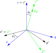
Figure 2: Transformation from a frame in which the $z^{\prime\prime}$-axis is aligned with the interstellar gas velocity vector into an arbitrary reference frame.

$$x^{\prime} = x^{\prime\prime}~{},$$

$$y^{\prime} = y^{\prime\prime}\cos\phi_{r}+z^{\prime\prime}\sin\phi_{r}~{},$$

$$z^{\prime} = -~{}y^{\prime\prime}\sin\phi_{r}+z^{\prime\prime}\cos\phi_{r}~{},$$ (69)

where

$$\sin\phi_{r} = \frac{\sqrt{v^{2}_{HX}+v^{2}_{HY}}}{v_{H}}~{},$$

$$\cos\phi_{r} = \frac{v_{HZ}}{v_{H}}~{}.$$ (70)

The second rotation is a rotation around the $z^{\prime}$-axis by the angle between $x$ and $x^{\prime}$.

$$x = x^{\prime}\cos\psi_{r}+y^{\prime}\sin\psi_{r}~{},$$

$$y = -~{}x^{\prime}\sin\psi_{r}+y^{\prime}\cos\psi_{r}~{},$$

$$z = z^{\prime}~{},$$ (71)

where

$$\sin\psi_{r} = \frac{v_{HX}}{\sqrt{v^{2}_{HX}+v^{2}_{HY}}}~{},$$

$$\cos\psi_{r} = \frac{v_{HY}}{\sqrt{v^{2}_{HX}+v^{2}_{HY}}}~{}.$$ (72)

Hence the transformation from the two primed frame into the unprimed frame is

$$x = x^{\prime\prime}\cos\psi_{r}+(y^{\prime\prime}\cos\phi_{r}+z^{\prime\prime}\sin\phi_{r})\sin\psi_{r}~{},$$

$$y = -~{}x^{\prime\prime}\sin\psi_{r}+(y^{\prime\prime}\cos\phi_{r}+z^{\prime\prime}\sin\phi_{r})\cos\psi_{r}~{},$$

$$z = -~{}y^{\prime\prime}\sin\phi_{r}+z^{\prime\prime}\cos\phi_{r}~{},$$ (73)

In order to find $\Omega$ and $i$ we can transform the coordinates of the unit vector $\vec{e}^{\prime\prime}_{N}$ $=$ ($\sin\Omega^{\prime\prime}$ $\sin i^{\prime\prime}$, $-\cos\Omega^{\prime\prime}$ $\sin i^{\prime\prime}$, $\cos i^{\prime\prime}$). We obtain

$$e_{NX} = \sin\Omega^{\prime\prime}\sin i^{\prime\prime}~{}\frac{v_{HY}}{\sqrt{v^{2}_{HX}+v^{2}_{HY}}}$$

$$+~{}\left(-\cos\Omega^{\prime\prime}\sin i^{\prime\prime}~{}\frac{v_{HZ}}{v_{H}}+\cos i^{\prime\prime}~{}\frac{\sqrt{v^{2}_{HX}+v^{2}_{HY}}}{v_{H}}\right)$$

$$\times~{}\frac{v_{HX}}{\sqrt{v^{2}_{HX}+v^{2}_{HY}}}~{},$$

$$e_{NY} = -\sin\Omega^{\prime\prime}\sin i^{\prime\prime}~{}\frac{v_{HX}}{\sqrt{v^{2}_{HX}+v^{2}_{HY}}}$$

$$+~{}\left(-\cos\Omega^{\prime\prime}\sin i^{\prime\prime}~{}\frac{v_{HZ}}{v_{H}}+\cos i^{\prime\prime}~{}\frac{\sqrt{v^{2}_{HX}+v^{2}_{HY}}}{v_{H}}\right)$$

$$\times~{}\frac{v_{HY}}{\sqrt{v^{2}_{HX}+v^{2}_{HY}}}~{},$$

$$e_{NZ} = \cos\Omega^{\prime\prime}\sin i^{\prime\prime}~{}\frac{\sqrt{v^{2}_{HX}+v^{2}_{HY}}}{v_{H}}+\cos i^{\prime\prime}~{}\frac{v_{HZ}}{v_{H}}~{}.$$ (74)

In this equation, Eq. (64) and Eq. (55) have to be used to determine the values of $\Omega^{\prime\prime}$ and $i^{\prime\prime}$. Since $\vec{e}_{N}$ $=$ ($\sin\Omega$ $\sin i$, $-\cos\Omega$ $\sin i$, $\cos i$), we can calculate $\Omega$ and $i$ from

$$\tan\Omega=-~{}\frac{e_{NX}}{e_{NY}}~{},$$ (75)

$$\cos i=e_{NZ}~{}.$$ (76)

Now we can find $\omega$ from Eqs. (3). One can easily verify that

$$J=S\cos\omega-I\sin\omega = \cos\Omega~{}v_{HX}+\sin\Omega~{}v_{HY}~{},$$ (77)

$$H=S\sin\omega+I\cos\omega = -~{}\sin\Omega~{}\cos i~{}v_{HX}$$ (78)

$$+~{}\cos\Omega~{}\cos i~{}v_{HY}$$

$$+~{}\sin i~{}v_{HZ}~{}.$$

Therefore

$$\sin\omega=\frac{HS-JI}{S^{2}+I^{2}}~{}~{}\mbox{and}~{}~{}\cos\omega=\frac{JS+HI}{S^{2}+I^{2}}~{}.$$ (79)

6.1 Perpendicular case

If the velocity vector of a neutral gas is perpendicular to the line of apsides, then $S$ $=$ 0 ($U$ $=$ 0) and the value of $S$ does not change with time. For this special case we obtain from Eqs. (35)–(36)

$$e^{2}_{1}=1-\frac{V^{2}}{v^{2}_{H}}~{},$$ (80)

$$e^{2}_{2}=0~{}.$$ (81)

Therefore the minimum eccentricity is 0 and the maximum eccentricity is $\sqrt{1-V^{2}/v^{2}_{H}}$. Using Eqs. (80)–(81) we obtain from Eqs. (31), (41) and (45) for the perpendicular case

$$C=\frac{V}{\sqrt{1-e^{2}}}~{},$$ (82)

$$I=-~{}\frac{v_{H}}{e~{}\sqrt{1-e^{2}}}~{}\frac{1-\frac{V^{2}}{v^{2}_{H}}}{2}~{}\sin\left(3\alpha v_{H}~{}\sqrt{\frac{a}{\mu_{\beta}}}~{}(t-t_{M})\right)~{},$$ (83)

$$e^{2}=\left(1-\frac{V^{2}}{v^{2}_{H}}\right)\cos^{2}\left(\frac{3\alpha v_{H}}{2}~{}\sqrt{\frac{a}{\mu_{\beta}}}~{}(t-t_{M})\right)~{}.$$ (84)

We mention that $C^{2}$ $+$ $I^{2}$ $=$ $v^{2}_{H}$ always holds for the perpendicular case.

For the inclination in the two primed frame, we have from Eq. (31) and Eq. (55)

$$\cos i^{\prime\prime}=\frac{V}{v_{H}\sqrt{1-e^{2}}}~{}.$$ (85)

Hence for $i^{\prime\prime}$ we obtain that $i^{\prime\prime}$ $\in$ (0, $\arccos(V/v_{H})$) for positive values of $V$ and $i^{\prime\prime}$ $\in$ ($\arccos(V/v_{H})$, $\pi$) for negative values of $V$.

Since $S$ $=$ 0 and $\sin i^{\prime\prime}$ $\neq$ 0, we obtain from the first of Eqs. (5) that $\sin\omega^{\prime\prime}$ $=$ 0. Therefore

$$\omega^{\prime\prime}=k_{6}\pi~{},$$ (86)

where $k_{6}$ is an integer.

Finally Eq. (56) for $\sin i^{\prime\prime}$ $\neq$ 0 yields that $\Omega^{\prime\prime}$ is a constant.

Now we find relations between the orbital elements in the unprimed frame for the special case $S$ $=$ 0. If we combine Eq. (16) for $S$ $=$ 0 with Eq. (18), we get

$$\frac{\cos\omega}{\sin\omega}~{}d\omega=-~{}\frac{\cos i}{\sin i}~{}di$$ (87)

which has the solution

$$|\sin i|~{}|\sin\omega|=d~{},$$ (88)

where $d$ is an integration constant. Since $i$ $\in$ (0, $\pi$), $\sin i$ $>$ 0. If $\sin\omega$ $\neq$ 0 initially, then $d$ $\neq$ 0 and therefore $\sin\omega$ can not change sign. Hence

$$\sin i~{}\sin\omega=l~{},$$ (89)

where $l$ is a constant. From Eq. (89) we can see that the orbital plane is only tilted back and forth around the line of apsides for the special case $S$ $=$ 0. The instantaneous value of $i$ can be determined from Eq. (76). In order to find $\Omega$ we combine Eq. (17) with Eq. (18). We get differential equation

$$\cos\omega~{}d\Omega=\frac{\sin\omega}{\sin i}~{}di~{}.$$ (90)

Equation (89) allows us to convert this expression into an equation for $\Omega(i)$ with solution

$$\tan(\Omega-\Omega_{0})=-~{}\frac{\sin\omega~{}\cos i}{\cos\omega}~{},$$ (91)

where $\Omega_{0}$ is the value of $\Omega$ for $i$ $=$ $\pi/2$.

7 Conclusion

We have investigated the long-term orbital evolution of a spherical dust particle perturbed by a small constant mono-directional force caused by a fast interstellar gas flow. The secular time derivatives of the particle’s Keplerian orbital elements were derived. We transformed the system of differential equations for the Keplerian orbital elements into a system of differential equations for the semi-major axis, eccentricity, and the radial, transversal, and normal components of the interstellar gas flow velocity vector determined at the pericentre of the particle’s orbit. In these new variables, the system of differential equations can be easily solved. The solution of the system was used in order to obtain the evolution of the Keplerian orbital elements in a reference frame in which the orbital elements are determined with respect to the plane perpendicular to the interstellar gas velocity vector. We found an explicit form for the time dependence of all Keplerian orbital elements in this reference frame. We generalized the expression for the time dependence of the longitude of the ascending node found by Belyaev and Rafikov (2010). We transformed newly found orbital elements into an arbitrary reference frame. This transformation gave us explicit time dependences of all Keplerian orbital elements in the arbitrary reference frame. The orbital elements of the dust particle in an arbitrary reference frame change periodically with a constant oscillation period or else remain constant. We determined the properties of the solution for the planar case and for the case in which the gas flow velocity vector is perpendicular to the line of apsides. We found the maximal and minimal values of the eccentricity in these cases. In the planar case, the particle’s orbit approaches the direction with maximal value of $I$. In the perpendicular case, the orbital plane is tilted back and forth around the line of apsides. We also confirmed the stationary solution found by Belyaev and Rafikov (2010). For the stationary solution, the orbital plane rotates around the line aligned with the gas flow velocity vector and going through the centre of gravity.

This solution can be applied also for the dust particles in the Solar system. If we consider icy particles with radii from 1 to 10 $\mu$m, then the solution is valid for orbits with semi-major axis from 200 to 3000 AU, approximately. More exact values of these limits depend on the radius of the particle. A maximal orbit eccentricity for which the solution is valid is smaller than approximately 0.8 and depends on the semi-major axis of the orbit and the particle’s radius (see Fig. 3). The period of change of the orbital elements for these orbits ranges from 10⁵ to 2 $\times$ 10⁶ years, approximately.

Appendix A Applicability of assumptions (f)–(h) in Solar system

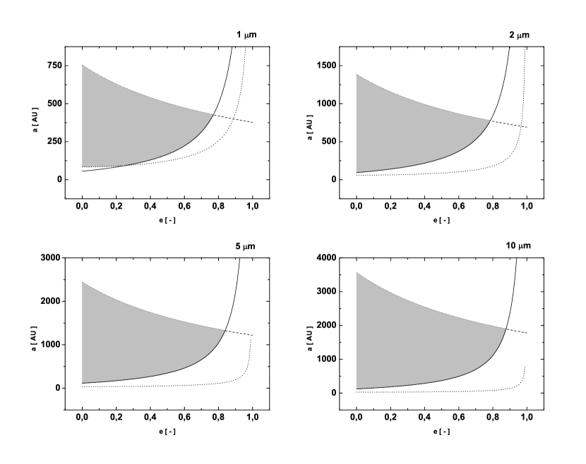
Figure 3: Allowed values of orbital semi-major axes and eccentricities in the $ae$-phase plane determined using the relations between the semi-major axis and eccentricity obtained from (93), (95) and (96). Dust particles have radius $R$ $\in$ {1 $\mu$m, 2 $\mu$m, 5 $\mu$m, 10 $\mu$m} and mass density $\varrho$ $=$ 1 g cm^-3 and $\bar{Q}^{\prime}_{pr}=1$. Dashed line indicates (93), solid line, (95) and dotted line, (96). The allowed region of the semi-major axes and eccentricities is depicted in grey.

Assumption (h) can be mathematically written as

$$\frac{\mu_{\beta}}{r^{2}}\gg\frac{c_{D}~{}n_{H}~{}m_{H}~{}A~{}v_{H}^{2}}{m}~{}.$$ (92)

This inequality must always hold during orbital evolution. The right-hand side of the inequality is a constant and the left-hand side is minimal at maximal $r$. Since we consider elliptical orbits, $r$ is maximal at the apocentre of the orbit. Therefore we will check this inequality at the apocentre. In the apocentre we can rewrite (92) as

$$\frac{\mu_{\beta}}{a^{2}~{}(1+e)^{2}}\gg\frac{3~{}c_{D}~{}n_{H}~{}m_{H}~{}v_{H}^{2}}{4~{}R~{}\varrho}~{},$$ (93)

where $a$ is the semi-major axis and $e$ is the eccentricity of the dust particle’s elliptical orbit. For a given particle this inequality determines the allowed $a$ and $e$ in the $ae$-phase plane.

Assumption (f) can be mathematically written as

$$|\vec{v}_{H}|\gg|\vec{v}|~{}.$$ (94)

Because the velocity of the particle is maximal at the pericentre of the orbit, we will check this inequality at the pericentre. In the pericentre we can rewrite (94) as

$$|\vec{v}_{H}|\gg\sqrt{\frac{\mu_{\beta}}{a}~{}\frac{1+e}{1-e}}~{}.$$ (95)

Similarly to (93), this inequality also determines the allowed $a$ and $e$ in the $ae$-phase plane.

Assumption (g) can be approximately mathematically written as (Wyatt and Whipple 1950)

$$-\left\langle\frac{da}{dt}\right\rangle_{PR}~{}\frac{1}{a}=\frac{\beta~{}\mu}{c~{}a^{2}}~{}\frac{2+3e^{2}}{(1-e^{2})^{3/2}}\ll b_{a}~{},$$ (96)

and

$$-\left\langle\frac{de}{dt}\right\rangle_{PR}~{}\frac{1}{e}=\frac{5~{}\beta~{}\mu}{2~{}c~{}a^{2}}~{}\frac{1}{(1-e^{2})^{1/2}}\ll b_{e}~{}.$$ (97)

Here, $b_{a}$ and $b_{e}$ determine the maximal values for the relative secular time derivatives. Inequalities (96) and (97) for a given particle, $b_{a}$ and $b_{e}$ determine the allowed $a$ and $e$ in the $ae$-phase plane. It is possible to show that for $b_{e}$ $>$ $5b_{a}/4$, the semi-major axis determined from (96) is always greater than the semi-major axis determined from (97) for $e$ $\in$ $[0,1)$. Therefore we will check only inequality (96). Using inequality (96) we take into account also the eccentricity of the particle’s orbits. This is a more general method than the method used by Belyaev and Rafikov (2010) who considered only circular orbits (see Eq. 26 in Belyaev and Rafikov 2010).

To obtain the conditions in the Solar system we used $L_{\odot}$ $=$ 3.842 $\times$ 10²⁶ W (Bahcall 2002), $c_{D}$ $=$ 2.6 (Banaszkiewicz et al. 1994; Scherer 2000; Pástor et al. 2011), $n_{H}$ $=$ 0.2 cm^-3 (Belyaev and Rafikov 2010) and $v_{H}$ $=$ 26 km s^-1 (e.g. Lallement 1996; Landgraf et al. 1999). In Fig. 3 four panels are depicted. Each of these corresponds to a different particle radius. We used particles with radius $R$ $\in$ {1 $\mu$m, 2 $\mu$m, 5 $\mu$m, 10 $\mu$m} and mass density $\varrho$ $=$ 1 g cm^-3 and $\bar{Q}^{\prime}_{pr}$ $=$ 1. Dependences between the semi-major axis and eccentricity are obtained from (93), (95) and (96). In (93) we assumed that the left-hand side must be at least 10 times greater than the right-hand side. For the equation obtained using this inequality we used the dashed line in Fig. 3. In (95) we also assumed that left-hand side must be at least 10 times greater than the right-hand side. In Fig. 3 this is depicted using a solid line. In (96) we assumed that $b_{a}$ $=$ 10^-6 year^-1 and the right-hand side must also be at least 10 times greater than the left-hand side. In Fig. 3 (96) is depicted useing a dotted line. The grey region in Fig. 3 represents values of semi-major axes and eccentricities in the $ae$-phase plane for which all three inequalities hold. In Fig. 3 we can see that assumptions (f)–(h) can be applied to the Solar system. If also assumptions (a)–(e) hold, then Eq. (5) can be used. Assumption (h) enables the use of perturbation theory.

Appendix B Connection with previous work

Pástor et al. (2011) take into account also the relative velocity $\vec{v}$ of the dust particle with respect to the star in the force caused by the neutral interstellar gas. The particle’s equation of motion has the following form

$$\frac{d\vec{v}}{dt}=-~{}\frac{\mu_{\beta}}{r^{3}}\vec{r}-c_{D}~{}\gamma_{H}~{}|\vec{v}-\vec{v}_{H}|~{}\left(\vec{v}-\vec{v}_{H}\right)~{}.$$ (98)

After expansion of the right-hand side of this equation into a series the linear term in the relative velocity is included in the calculation of the secular time derivatives of the Keplerian orbital elements. The result for the secular time derivative of the semi-major axis is

$$\left\langle\frac{da}{dt}\right\rangle = -~{}2~{}a~{}c_{D}~{}\gamma_{H}~{}v_{H}^{2}~{}\sqrt{\frac{p}{\mu_{\beta}}}~{}\sigma~{}\Biggl{\{}1+\frac{1}{v_{H}^{2}}$$ (99)

$$\times~{}\Biggl{[}I^{2}-(I^{2}-S^{2})\frac{1-\sqrt{1-e^{2}}}{e^{2}}\Biggr{]}\Biggr{\}}~{},$$

where

$$\sigma=\frac{\sqrt{\mu_{\beta}/p}}{v_{H}}~{}.$$ (100)

From Eq. (99) we can see that the secular time derivative of the semi-major axis is proportional to the value of the semi-major axis (the value of $\sqrt{p/\mu_{\beta}}~{}\sigma$ is independent of the semi-major axis). The term within the square brackets ($SB$) in Eq. (99) can be written as

$$SB=I^{2}-(I^{2}-S^{2})\frac{1-\sqrt{1-e^{2}}}{e^{2}}=\frac{1-\sqrt{1-e^{2}}}{e^{2}}~{}(I^{2}\sqrt{1-e^{2}}+S^{2})\geq 0~{}.$$ (101)

The secular semi-major axis is a decreasing function of time.

Now, we find the maximal possible decrease of the secular semi-major axis. Because terms the multiplied by $S^{2}$ and $I^{2}$ are both positive, we obtain the maximal value of $SB$ for the orbit orientation characterized by $C$ $=$ 0. If $C$ $=$ 0, then $S^{2}$ $+$ $I^{2}$ $=$ $v_{H}^{2}$. Using this, the value of $SB$ can be written as

$$SB=\frac{1-\sqrt{1-e^{2}}}{e^{2}}~{}[v_{H}^{2}\sqrt{1-e^{2}}+S^{2}(1-\sqrt{1-e^{2}})]~{}.$$ (102)

Here, $v_{H}^{2}$ is constant. Therefore, we obtain the maximal value of $SB$ for the orbit orientation characterized by $S^{2}$ $=$ $v_{H}^{2}$. Hence, the maximal value of $SB$ is

$$SB=v_{H}^{2}~{}\frac{1-\sqrt{1-e^{2}}}{e^{2}}=v_{H}^{2}~{}g(e)~{}.$$ (103)

In order to find the behaviour of the function $g(e)$ we can write

$$\frac{dg(e)}{de}=\frac{2-e^{2}-2\sqrt{1-e^{2}}}{e^{3}\sqrt{1-e^{2}}}~{},$$ (104)

$$\frac{dg_{1}(e)}{de} = \frac{d}{de}~{}\bigl{(}2-e^{2}-2\sqrt{1-e^{2}}\bigr{)}$$ (105)

$$= -2~{}e+\frac{2~{}e}{\sqrt{1-e^{2}}}\geq 0~{}.$$

Because $dg_{1}(e)/de$ $\geq$ 0, $g_{1}(e)$ is an increasing function of the eccentricity. The value of $g_{1}(0)$ is 0. Therefore, $g_{1}(e)$ is positive for $e$ $\in$ (0, 1]. If $g_{1}(e)$ is positive, then $dg(e)/de$ $>$ 0. Because $dg(e)/de$ $>$ 0, the function $g(e)$ is an increasing function of the eccentricity for $e$ $\in$ (0, 1]. The function $g(e)$ has its maximal value for $e$ $=$ 1. Therefore the maximal value of $SB$ is

$$SB_{\mbox{max}}=v_{H}^{2}~{}.$$ (106)

Hence, the maximal possible decrease of the secular semi-major axis is

$$\left\langle\frac{da}{dt}\right\rangle_{\mbox{max}}=-~{}4~{}a~{}c_{D}~{}\gamma_{H}~{}v_{H}^{2}~{}\sqrt{\frac{p}{\mu_{\beta}}}~{}\sigma~{}.$$ (107)

R	$T_{a}$
[$\mu$m]	$\left[10^{3}\atop\mbox{years}\right]$
1	46.7
2	93.4
5	233.4
10	466.8

Table 2: Time intervals $T_{a}$ after which the decrease of the semi-major axis is smaller than 10% ($c_{a}$ $=$ 0.9) for particles with $R$ $\in$ {1 $\mu$m, 2 $\mu$m, 5 $\mu$m, 10 $\mu$m} and mass density $\varrho$ $=$ 1 g cm^-3 in the Solar system.

We define a time interval $T_{a}$ during which we suppose that the semi-major axis is approximately constant. For a given value of the semi-major axis we have

$$\frac{a+\left\langle\frac{da}{dt}\right\rangle_{\mbox{max}}~{}T_{a}}{a}=\mbox{constant}=c_{a}\approx 1~{}.$$ (108)

Because we use the maximal possible decrease of the secular semi-major axis, the left-hand side of Eq. (108) will be even closer to unity for the real secular time derivative of the semi-major axis. However

$$\frac{T_{a}}{T_{e}}=\frac{3~{}T_{a}~{}\alpha~{}v_{H}}{2~{}\pi}~{}\sqrt{\frac{a}{\mu_{\beta}}}$$ (109)

(see Eq. 42) is proportional to $a^{1/2}$. Therefore, for larger semi-major axes we obtain more eccentricity periods in the same time interval $T_{a}$. Therefore the theory with the equation of motion considered in the form of Eq. (5) is better applicable for larger semi-major axes. We can calculate the values of $T_{a}$ from Eq. (108). If we use $c_{a}$ $=$ 0.9, then we obtain for dust particles with $R$ $\in$ {1 $\mu$m, 2 $\mu$m, 5 $\mu$m, 10 $\mu$m} and mass density $\varrho$ $=$ 1 g cm^-3 in the Solar system (see Appendix A) the values of $T_{a}$ shown in Table 2.