A novel approach for accurate radiative transfer in cosmological hydrodynamic simulations

Abstract

We present a numerical implementation of radiative transfer based on an explicitly photon-conserving advection scheme, where radiative fluxes over the cell interfaces of a structured or unstructured mesh are calculated with a second-order reconstruction of the intensity field. The approach employs a direct discretisation of the radiative transfer equation in Boltzmann form with adjustable angular resolution that in principle works equally well in the optically thin and optically thick regimes. In our most general formulation of the scheme, the local radiation field is decomposed into a linear sum of directional bins of equal solid-angle, tessellating the unit sphere. Each of these “cone-fields” is transported independently, with constant intensity as a function of direction within the cone. Photons propagate at the speed of light (or optionally using a reduced speed of light approximation to allow larger timesteps), yielding a fully time-dependent solution of the radiative transfer equation that can naturally cope with an arbitrary number of sources, as well as with scattering. The method casts sharp shadows, subject to the limitations induced by the adopted angular resolution. If the number of point sources is small and scattering is unimportant, our implementation can alternatively treat each source exactly in angular space, producing shadows whose sharpness is only limited by the grid resolution. A third hybrid alternative is to treat only a small number of the locally most luminous point sources explicitly, with the rest of the radiation intensity followed in a radiative diffusion approximation. We have implemented the method in the moving-mesh code AREPO, where it is coupled to the hydrodynamics in an operator splitting approach that subcycles the radiative transfer alternatingly with the hydrodynamical evolution steps. We also discuss our treatment of basic photon sink processes relevant for cosmological reionisation, with a chemical network that can accurately deal with non-equilibrium effects. We discuss several tests of the new method, including shadowing configurations in two and three dimensions, ionised sphere expansion in static and dynamic density field and the ionisation of a cosmological density field. The tests agree favourably with analytic expectations and results based on other numerical radiative transfer approximations.

1 Introduction

The transport of radiation and its interaction with matter is of fundamental importance in astrophysics, playing a crucial role in the formation and evolution of objects as diverse as stars, black holes, or galaxies. It would therefore be highly desirable to be able to calculate radiative transfer (RT) processes with equal accuracy and ease as ordinary hydrodynamical and gravitational dynamics. Unfortunately, the difficult mathematical structure of the radiative transfer equation, which takes the form of a partial differential equation in six dimensions (3 spatial dimensions, 2 angular dimensions, 1 frequency dimension) makes this an extremely challenging goal. In fact, the RT problem is so hard, even in isolation, that coupled radiation hydrodynamics methods are still in their infancy in cosmology thus far.

However, a large array of different approximations to the RT problem have been developed over the years, which are often specifically tuned to the requirements and characteristics of particular types of problems, and in many cases are applied to static density fields only. In this study, we are primarily concerned with RT in calculations of cosmological reionisation and in star formation, leaving aside other important areas such as stellar spectra and atmospheres. Especially for the reionisation problem, recent years have seen a flurry of activity in the development of new RT solvers that are well suited to this problem. These numerical methods include long and short characteristics schemes, ray-tracing, moment methods and direct solvers, and other particle- or Monte-Carlo-based transport methods. In the following we briefly describe these schemes.

In the long characteristics method (Mihalas & Weibel Mihalas, 1984; Abel et al., 1999; Sokasian et al., 2001; Cen, 2002; Abel & Wandelt, 2002; Razoumov & Cardall, 2005; Susa, 2006), each source cell in the computational volume is connected to all other relevant cells. Then the RT equation is integrated individually from that cell to each of the selected cells. While this method is relatively simple and straight-forward, it is also very time consuming, since it requires ${\cal O}(N^{2})$ interactions between the cells. Moreover, parallelisation of this approach is cumbersome and requires large amounts of data exchange between the different processors.

Short characteristics methods (Kunasz & Auer, 1988; Nakamoto et al., 2001; Mellema et al., 1998; Mellema et al., 2006; Shapiro et al., 2004; Whalen & Norman, 2006; Alvarez et al., 2006; Ahn & Shapiro, 2007; Altay et al., 2008; Ciardi et al., 2001; Maselli et al., 2003; Gritschneder et al., 2009; Cantalupo & Porciani, 2010; Hasegawa & Umemura, 2010; Baek et al., 2009) try to gain efficiency by integrating the equation of radiative transfer only along lines that connect nearby cells, and not to all other cells in the computational domain. This reduces the redundancy of the computations and makes the scheme easier to parallelise.

A widely used incarnation of the long-characteristics method are so-called ray-tracing schemes. Here a discrete number of rays is traced from each source, along which the RT equation is integrated in 1D, considering absorptions and recombinations. As the angular resolution decreases with increasing distance from the source, rays may be split into subrays (e.g. Abel & Wandelt, 2002; Trac & Cen, 2007) for higher efficiency. The ray-tracing itself can be performed either on grids (Mellema et al., 2006; Whalen & Norman, 2006) or using particles as interpolation points (Baek et al., 2009; Gritschneder et al., 2009; Altay et al., 2008). Other innovative methods trace photons on unstructured grids, for example Delaunay tessellations, that are adapted to the mean photon optical depth of the gas (Rijkhorst et al., 2006; Paardekooper et al., 2010; Ritzerveld & Icke, 2006).

Stochastic integration methods, specifically Monte Carlo methods, employ a ray-casting strategy where the rays are discretised into photon packets (Maselli et al., 2003; Baek et al., 2009) or particles (Nayakshin et al., 2009). For each photon packet, its frequency and its direction of propagation are determined by sampling the appropriate distribution function of the emitters that have been assigned in the initial conditions. A particular advantage of this approach is that comparatively few approximations to the radiative transfer equations need to be made, so that the quality of the results is primarily a function of the number of photon packets employed, which can be made larger in proportion to the CPU time spent. A disadvantage of these schemes is the comparatively high computational cost and the sizable level of noise in the simulated radiation field, which only slowly diminishes as more photon packets are used. The ‘cone’ transport scheme of (Pawlik & Schaye, 2008), where radiation is directly transferred between particles, tries to improve on these limitations. If needed, this method can also create further sampling points dynamically to improve the resolution locally.

Using moments of the radiative transfer equations instead of the full set of equations can lead to very substantial simplifications that can drastically speed up the calculations. In this approach, the radiation is represented by its mean intensity field throughout the computational domain, which is evolved either in a diffusion approximation or based on a suitably estimated local Eddington tensor (Gnedin & Abel, 2001; Aubert & Teyssier, 2008; Petkova & Springel, 2009; Finlator et al., 2009). Instead of following rays, the moment equations are solved directly on the grid, or in a mesh-less fashion on a set of sampling particles. Due to its local nature, the moment approach is comparatively easy to parallelise, but its accuracy is highly problem dependent, making it difficult to judge whether the simplifications employed still provide sufficient accuracy. The simplest and most popular moment method is radiative diffusion (e.g. Whitehouse et al., 2005; Reynolds et al., 2009), where the RT equation is approximated in terms of an integrated energy density in each discretised mass or volume element, and this radiation energy density is then evolved through the flux-limited diffusion approximation, where the flux limiter is introduced to prevent the occurrence of transfer speeds larger than the speed of light. While the diffusion approximation works very well in the optically thick regime, its accuracy is hard to judge in general situations.

A comparison of the relative accuracy of these established RT methods has been carried out in the “cosmological radiative transfer comparison project” (Iliev et al., 2006; Iliev et al., 2009), where a subset of the above implementations has been compared on a variety of simple test problems. Such a comparison is particularly useful as the lack of known analytic solutions for the RT problem, except for a small number of simple situations, makes the validation of a RT method quite difficult. Reassuringly, the comparison project found in most cases reasonably good agreement between the different methods, but it also highlighted that each of the different techniques shows individual strengths and weaknesses, providing ample motivation to search for still better methods.

It is the goal of this study to propose a new numerical scheme for RT that is competitive with the best of the known methods in terms of accuracy and general applicability, but is also fast enough to allow self-consistent radiation-hydrodynamic simulations in the context of cosmological reionisation and star formation problems. We also aim to couple the method to the new moving-mesh code AREPO (Springel, 2010), which solves the equations of hydrodynamics on an unstructured Voronoi mesh that moves with the flow and automatically adapts its resolution to the gravitational clustering of matter. This mesh-based code computes hydrodynamics similar to high-accuracy Eulerian codes on Cartesian grids, but it features reduced advection errors when the flow velocity is large.

Our new method is based on a radiation advection technique where a second-order accurate, piece-wise linear reconstruction of the photon intensity field is used to estimate upwind photon fluxes for each face of the mesh. If there is only a single point source, such a scheme can exploit the fact that the local streaming direction of the photons is known everywhere – it is along the ray from the source’s position to the local coordinate. If there are multiple sources, the radiation field can be treated equally accurately by decomposing it into a linear sum for each source, and treating each component independently. Alternatively, we introduce a direct discretisation of angular space, allowing a description of arbitrary source fields, albeit at the cost of a finite angular resolution. We note that in all these variants the conservation of photon number is manifest in the transport step. We treat the source terms and the coupling to the hydrodynamics in an operator split approach, where the emission, advection, and absorption of radiation are calculated in separate steps. This makes our approach fully photon conserving, which is especially useful for the cosmic reionisation problem, as it ensures that all photons emitted by an ionising source are really used up in exactly one ionisation event.

We note that the advection scheme discussed in this paper normally propagates the photons at their physical speed of light, based on an explicit time integration scheme. While this has the advantage of allowing general, fully time-dependent radiative transfer simulations, it can make them computationally very expensive due to the required small Courant time steps. This can however be greatly alleviated by using a reduced speed of light approximation (Gnedin & Abel, 2001), which allows much larger timesteps while still preserving the speed of cosmological ionisation fronts (I-fronts). With this approximation, it then becomes possible to calculate high-resolution cosmological radiation hydrodynamics simulations of structure formation that simultaneously account for cosmic reionisation, with no restriction on the number of sources.

In Section 2 of this paper, we present our methodology in detail. We first give a brief introduction to the RT equation in Section 2.1. Then we discuss three variants of our solution method for the radiation advection equation in Sections 2.2, 2.3, and 2.4. In Section 2.5, we briefly describe our treatment of emission and absorption processes, with an emphasis on the hydrogen chemistry relevant for the cosmic reionisation problem, and in Section 2.6 we specify our formulation of photo-heating and radiative cooling. Issues of time stepping and code implementation are discussed in Sections 2.7 and 2.8. We move on to a presentation of basic test results in Section 3, starting with a variety of shadowing (Section 3.1) and Strömgren sphere tests (Section 3.2). We then consider the more demanding tests of I-front trapping in Section 3.3, the ionisation of a cosmological density field in Section 3.4, and an ionisation problem with dynamic density field in Section 3.5. Finally, we present our conclusions in Section 4.

2 An advection solver for the radiative transfer problem

2.1 The radiative transfer equation

Let us briefly discuss different forms of the RT equation, which is helpful to clarify how our new method differs from other approaches, and for specifying our notation. Let $f_{\gamma}\equiv f_{\gamma}(t,{\bf x},{\bf p})$ be the photon distribution function for comoving coordinate ${\bf x}$ and photon momentum

$${\bf p}=a\frac{h\nu}{c}{\bf\hat{n}}\,,$$ (1)

where $a\equiv a(t)$ is the cosmological scale factor, $h$ is the Planck constant, $\nu$ is the frequency of the photons, and ${\bf\hat{n}}$ is the unit vector in the direction of photon propagation. Then the number of photons in some part of the Universe is

$$N_{\gamma}=\int{\rm d}{\bf x}\,{\rm d}{\bf p}\,f_{\gamma}(t,{\bf x},{\bf p})\,.$$ (2)

We can quite generally write the phase-space continuity equation for the distribution function $f_{\gamma}$ of photons as

$$\frac{\partial f_{\gamma}}{\partial t}+\frac{\partial}{\partial{\bf x}}(\dot{{\bf x}}f_{\gamma})+\frac{\partial}{\partial{\bf p}}(\dot{{\bf p}}f_{\gamma})=\left.\frac{\partial f_{\gamma}}{\partial t}\right|_{\rm sources}-\left.\frac{\partial f_{\gamma}}{\partial t}\right|_{\rm sinks}.$$ (3)

In this Boltzmann-like transport equation, the source and sink terms on the right-hand side of the equation represent photon emission and absorption processes, respectively. If we neglect gravitational lensing effects, individual photons propagate along straight lines with conserved momenta, i.e. we have ${\bf\dot{x}}=(c/a){\bf\hat{n}}$ and ${\bf\dot{p}}=0$. The transport equation hence simplifies to

$$\frac{\partial f_{\gamma}}{\partial t}+\frac{c}{a}\frac{\partial}{\partial{\bf x}}({\bf\hat{n}}f_{\gamma})=\left.\frac{\partial f_{\gamma}}{\partial t}\right|_{\rm sources}-\left.\frac{\partial f_{\gamma}}{\partial t}\right|_{\rm sinks}.$$ (4)

Normally, a direct use of equation (4) through a discretisation of phase-space is considered prohibitively expensive due to the high-dimensionality of the problem. However, if only monochromatic radiation is considered, which is often sufficient, the momentum-space dimensions reduce to just two angular coordinates. If furthermore only a relatively coarse angular resolution for the photon transport is sufficient, then the $4\pi$ solid angle described by these angular dimensions may be discretised into a limited set of cones, say up to 10-100, at which point a brute-force solution of equation (4) on a 3D mesh becomes computationally feasible and attractive, as we shall argue here.

Before we discuss this in more detail, let us first briefly recall for clarity how the specific intensity $I_{\nu}$ that is normally used in RT studies relates to equation (4). We can define the specific radiation intensity $I_{\nu}$ in a certain direction ${\bf\hat{n}}$ through the energy $\Delta E_{\nu}=I_{\nu}\Delta\nu\Delta A\Delta\Omega\Delta t$ of photons that pass through a physical area $\Delta A$ normal to ${\bf\hat{n}}$ and within solid angle $\Delta\Omega$ around ${\bf\hat{n}}$, over a time interval $\Delta t$ and in a frequency bin $\Delta\nu$. With this definition, the specific intensity $I_{\nu}$ is then related to the photon distribution function $f_{\gamma}$ as

$$I_{\nu}=h\nu f_{\gamma}\frac{{\rm d}^{3}x\,{\rm d}^{3}p}{{\rm d}\nu\,{\rm d}\Omega\,{\rm d}A\,{\rm d}t}=\frac{h^{4}\nu^{3}}{c^{2}}f_{\gamma}\,.$$ (5)

Substituting into equation (4), and writing the absorption and emission terms in their conventional form, one obtains the cosmological RT equation in the form

$$\frac{1}{c}\frac{\partial I_{\nu}}{\partial t}+\frac{{\bf\hat{n}}}{a}\frac{\partial I_{\nu}}{\partial{\bf x}}-\frac{H(a)}{c}\left(\nu\frac{\partial I_{\nu}}{\partial\nu}-3I_{\nu}\right)=-\kappa_{\nu}I_{\nu}+j_{\nu}\,,$$ (6)

where $\kappa_{\nu}$ is the absorption coefficient, $j_{\nu}$ is the emission coefficient, and $H(a)$ is the Hubble rate. Defining the solid angle averaged intensity as

$$J_{\nu}=\frac{1}{4\pi}\int{\rm d}\Omega\,I_{\nu},$$ (7)

we can calculate the physical photon number density from the specific intensity as

$$n_{\gamma}^{\rm phys}=\frac{1}{c}\int\frac{4\pi J_{\nu}}{h\nu}\,{\rm d}\nu.$$ (8)

Another equivalent way to obtain the photon number density is simply to integrate the distribution function,

$$n_{\gamma}=\int{\rm d}{\bf p}\,f_{\gamma}(t,{\bf x},{\bf p}),$$ (9)

which yields the comoving number density of photons, $n_{\gamma}=a^{3}n_{\gamma}^{\rm phys}$. This highlights again that describing the radiation field with the arguably more familiar RT equation (6), or with the distribution function and the Boltzmann-like equation (4), is fully equivalent. In this paper, we will mostly work in the latter formulation.

In general, to solve the RT problem on some discretised mesh, we can split off the source and sink terms and treat them separately in the time integration. In such an operator splitting approach, known as Strang splitting, we are basically left with two separate problems that are interleaved in the time integration, one is to follow the conservative transport of photons on the mesh, the other is the local updating of the photon density field through the source and sink terms. In the following, we first focus on the conservative transport problem, which is where the primary computational challenge lies.

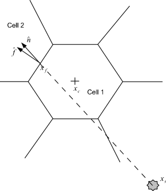
Figure 1: A simple sketch showing the geometry involved in our advection scheme for a single point source at coordinate ${\bf x}_{s}$. Here ${\bf\hat{n}}$ is the photon propagation direction, ${\bf\hat{f}}$ is the normal vector of a face of a cell, ${\bf x}_{c}$ is the center of mass of the corresponding cell and ${\bf x}_{f}$ is the center of mass of the face for which the photon flux is calculated.

2.2 Transferring radiation by advection for point sources

Suppose for the moment that we know at a given point in space that all photons stream in the same direction ${\bf\hat{n}}$. This is for example the case if there is a single point source at coordinate ${\bf x}_{s}$ (i.e. no other sources and no scattering are present). For simplicity, we shall also restrict ourselves to a spatially invariant photon momentum spectrum. One then obtains a simple advection equation for the comoving photon density $n_{\gamma}$:

$$\frac{\partial n_{\gamma}}{\partial t}+\frac{c\,{\bf\hat{n}}}{a}\cdot\nabla n_{\gamma}=0,$$ (10)

where the local advection direction ${\bf\hat{n}}$ is known at every point ${\bf x}$ and is simply given by

$${\bf\hat{n}}({\bf x})=\frac{{\bf x}-{\bf x}_{s}}{|{\bf x}-{\bf x}_{s}|}.$$ (11)

This advection is conservative and may be solved with the techniques commonly employed to treat the hyperbolic conservation laws of ideal fluid dynamics on spatial meshes. Indeed, this is the approach we are going to employ: we shall use a conservative transport scheme based on a second-order accurate upwind method that is inlined with the hydrodynamic calculations of our unstructured moving-mesh hydrodynamics code AREPO, which is described in some more detail below. It is important to note that knowledge of the local number density field of photons combined with the source location ${\bf x}_{s}$ is sufficient to accurately solve the radiative transport, simply because this information suffices to specify the photon streaming direction at every point in space. Apart from the spatial discretisation, no approximations need to be made for the case of a single monochromatic point source in this treatment.

In practice, we use a second-order accurate spatial reconstruction technique to convert photon numbers $N_{i}$ stored for each cell $i$ of a given mesh into a photon density field. For every cell, we first obtain an estimate $\left<{\bf\nabla}n_{\gamma}\right>_{i}$ for the gradient of $n_{\gamma}$, which allows a piece-wise linear conservative reconstruction of the photon density field, in the form

$$n_{\gamma}({\bf x})=\left<n_{\gamma}\right>_{i}+\left<{\bf\nabla}n_{\gamma}\right>_{i}({\bf x}-{\bf x}^{c}_{i}),\;\;\;\;{\rm for}\;{\bf x}\in{\rm cell}\;i.$$ (12)

Here $\left<n_{\gamma}\right>_{i}=N_{i}/V_{i}$ is the mean photon number density in the cell with center-of-mass ${\bf x}^{c}_{i}$ and volume $V_{i}$. As illustrated in the sketch of Figure 1, for every face centroid ${\bf x}_{f}$ of the mesh, we can then identify the upwind side of the photon flow, based on the sign of the dot product between face normal ${\bf\hat{f}}$ and the photon streaming direction ${\bf\hat{n}}=({\bf x}_{f}-{\bf x}_{s})/|{\bf x}_{f}-{\bf x}_{s}|$. This allows us to estimate the photon flux $F_{\gamma}$ over the face as

$$F_{\gamma}=\frac{c}{a}\,({\bf f}\cdot{\bf\hat{n}})\,n_{\gamma}({\bf x}_{f}),$$ (13)

where the photon density $n_{\gamma}({\bf x}_{f})$ at the face centroid is estimated based on the linear reconstruction of the cell on the upwind side. If the face has comoving area $A$, the number of photons exchanged during time $\Delta t$ between the cells that share the face is then given by

$$\Delta N_{\gamma}=F_{\gamma}A\Delta t.$$ (14)

Due to the pairwise exchange of photons, the conservation of total photon number is manifest, which is important for guaranteeing that I-fronts propagate at their physical speeds. We note that in our code the mesh is composed of Voronoi cells (of which a Cartesian mesh is a special case), but this is not important for the general approach.

There are two important caveats with this transport scheme, which need to be pointed out. One is that this explicit transport scheme requires a time step that is given by a local Courant criterion for the photons, which can become very small due to the high speed of light. For reionisation problems, this can however be circumvented with the reduced speed of light approximation, which we will discuss in more detail later on. The other caveat is that close to a point source the mesh resolution will always be coarse, so that our use of a single Gauss point per mesh face may introduce sizable errors in the discretised advection fluxes. This can happen when the opening angle under which a mesh face is seen by the point source is large, so that adopting a single propagation direction for the entire face is inaccurate. As a result, isophots of the radiation field produced by the point source may then deviate from sphericity with distortions that reflect the local geometry of the mesh around the point source. We have found however that this problem can be cured quite effectively by injecting the photons of the source in a kernel-weighted fashion over 2-3 mesh cells or so. With such slightly extended sources, the above scheme is able to quite accurately treat single point sources.

Figure 2: Sketch that illustrates the linear summation principle used to treat the radiative transfer for multiple sources. Here ${\bf\hat{n}}_{1}$ and ${\bf\hat{n}}_{2}$ are the photon propagation directions from the two sources, as seen from the center ${\bf x}_{f}$ of a face with normal vector ${\bf\hat{f}}$. The total flux passing through the face is then computed as a linear sum of the contributions from the partial fields created by each source.

The approach can also be straightforwardly extended to multiple point sources simply by linear superposition of the radiation fields produced by each of the individual sources, as sketched in Figure 2. This means that the advection equation is solved for the radiation field of each source separately. This obviously involves a computational and storage cost that scales with the number of sources, but if the number of sources is small, this is an interesting technique for certain applications due to its high accuracy. As we show in our test problems, the method in particular is able to accurately cast shadows, and unlike for example in the optically thin variable Eddington tensor approximation (OTVET), there is no accuracy-degrading mutual influence of multiple sources on each other.

However, for a large number of ionising sources, the linear superposition approach will quickly become infeasible. For example, in large cosmological simulations, we would like to allow every star particle to act as a source of ionising radiation. Here we obviously cannot decompose the radiation field into all its single point sources, instead, we need to employ another decomposition. We have actually developed two possible schemes for this, which we describe in the following.

2.3 A hybrid between point-source treatment and local diffusion

One possibility to address the multiple point sources problem is to only retain a finite number $N_{\rm br}$ of locally brightest sources in an explicit treatment, while all the remaining sources are lumped together into a background radiation field that is treated with radiative diffusion. The idea here is that especially in cosmic reionisation problems the local ionisation “bubble” is expected to be driven primarily by one or a few sources, and only at very late stages, multiple sources may become visible at a given point, but then reionisation has largely completed already anyway. By making the set of sources that are treated exactly as point sources spatially variable, we should then get a quite accurate approximation of the reionisation phenomenon even for moderate values of $N_{\rm br}$. Since in the limit of large $N_{\rm br}$, the scheme will become essentially exact (apart from spatial discretisation errors), the degree to which imposing a limiting value for $N_{\rm br}$ affects the results can be readily tested.

We will discuss some results obtained with this approach later on, but we note that it clearly involves several complication when applied in practice. First of all, the need to allow a local change of the list of bright sources requires that one keeps track of all locally incoming fluxes of radiation, sorting them appropriately, and matching them through the use of unique source identifiers to the already stored radiation intensities from the previous step. Also, since neighboring cells may have different source lists, a matching procedure is required for gradient estimates, with the additional complication that the accuracy of the gradients will be reduced at “domain boundaries”, i.e. regions of the mesh that differ in their assessment what the locally most important $N_{\rm br}$ point sources are. Furthermore, if the number of sources is very large and spread out in space (e.g. the individual stars in galaxies), the injection of photons needs to be treated in some sort of clustered fashion, otherwise faint individual sources may not be able to compete with the $N_{\rm br}$ bright sources already stored locally, so that they are channeled into the radiatively treated flux reservoir right away without having a chance to build up to a significant source when combined with the potentially many nearby sources that are equally faint. Finally, one also needs a separate radiative diffusion solver, which requires a small timestep for stability when integrated explicitly in time, as we do here. For all these reasons, we actually favour in most applications our second approach for treating a large number of sources, which is facilitated by discretising the solid angle explicitly, as we describe next.

2.4 Full angular discretisation and cone transport

For general radiation fields we seek a method that can directly represent the angular distribution of the local radiation field. This can, for example, be done in terms of moments of the radiation field. However, we here want to propose a more flexible approach that is based on a direct angular discretisation of the photon space. To this extent, we can decompose the full solid angle into a set of cones of equal size, for example based on the well-known HEALPIX (Górski et al., 2005) tessellation of the unit-sphere, which we shall use in the following. Our strategy could however be straightforwardly generalised also for other discretisations of angular space. In HEALPIX, the unit sphere is decomposed into $N_{\rm pix}=12\,N_{\rm side}^{2}$ patches of equal solid angle (which we call “cones” for simplicity, even though they are not exactly axi-symmetric), each centred around a central direction ${\bf\hat{n}}_{j}$, where $j=1\ldots N_{\rm pix}$. We now linearly decompose the radiation field $f_{\gamma}$ into $N_{\rm pix}$ components, each containing the photons that propagate along a direction within the corresponding cone:

$$f_{\gamma}({\bf x},{\bf\hat{n}})=\sum_{j}f_{\gamma}^{j}({\bf x},{\bf\hat{n}}),$$ (15)

where $f_{\gamma}^{j}({\bf x},{\bf\hat{n}})=0$ if the photon direction ${\bf\hat{n}}$ lies outside of $\Delta\Omega_{j}$ around ${\bf\hat{n}}_{j}$. The basic simplification we now make is that we assume that each of the partial radiation fields, $f_{\gamma}^{j}({\bf x},{\bf\hat{n}})$, can be taken to be constant as a function of direction within the corresponding cone. Or in other words, each of the partial fields $f_{\gamma}^{j}({\bf x},{\bf\hat{n}})$ describes the intensity of a homogeneously illuminated beam of opening angle $\Delta\Omega_{j}$ around direction ${\bf\hat{n}}_{j}$, emanating from the local coordinate ${\bf x}$. Our goal is now to generalise the radiation advection scheme for point sources outlined above such that it can accurately transport the radiation cones occurring in this discretisation.

If we simply transport one of the partial radiation fields $f_{\gamma}^{j}$ locally always along the primary direction of its cone, i.e.

$$\frac{\partial f_{\gamma}^{j}}{\partial t}+\frac{c\,{\bf\hat{n}}_{j}}{a}\cdot\nabla f_{\gamma}^{j}=0,$$ (16)

we will invariably observe a central “focusing effect”, i.e. the radiation emanating from a point will not illuminate the finite solid angle $\Delta\Omega_{j}$ homogeneously, but rather tend to concentrate along the primary axis of the cone. It is clear that this “focusing effect” arises from the parallel transport described by equation (16); instead of transporting the photon field over different directions that are uniformly spread over the finite solid angle, all of the photons are transported along the single direction ${\bf\hat{n}}_{j}$, with any residual angular spread around ${\bf\hat{n}}_{j}$ arising only from numerical diffusion due to the finite mesh resolution.

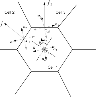
Figure 3: This sketch illustrates the geometry and the vectors involved in our “cone transport”, where the angular space is discretised into regions of equal angle (in 2D) or solid angle (in 3D). In this example, only four cones in in 2D are used. The photon field is linearly decomposed into radiation fields corresponding to the four cones, which have symmetry axes ${\bf\hat{n}}_{1},\,{\bf\hat{n}}_{2},\,{\bf\hat{n}}_{3},\,...\,{\bf\hat{n}}_{N}$, where $N$ is the number of discrete cones or angles, i.e. $N=4$ in the sketch. At each face of the mesh (here the normal vectors ${\bf\hat{f}}_{1}$ and ${\bf\hat{f}}_{2}$ are shown), photon fluxes for each of the partial fields are estimated. The photon propagation direction is taken to be parallel to the gradient of the total radiation intensity field, constrained to lie within the opening angle of the corresponding cone.

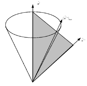
Figure 4: A sketch illustrating the construction of the vector given by equation (20). The symmetry axis of the solid-angle cone $j$ is given by ${\bf\hat{n}}_{j}$, while the gradient direction is ${\bf\hat{n}}_{j}^{\prime}$. If the latter lies outside the cone, it is projected onto the cone to yield direction $({\bf\hat{n}}_{j}^{\prime})_{\rm new}$, which is then used in the local advection step for the cone’s radiation field.

One may try to fix this problem by somehow randomising the direction within the corresponding cone taken in single transport steps, or by using higher-order quadratures in integrating the fluxes arising for a given mesh geometry. However, we have found that a simple trick can be used to resolve this issue, and to obtain close to perfect results even for unfavourable mesh geometries. To this end, we replace the local advection direction ${\bf\hat{n}}_{j}$ appearing in equation (16) with a modified direction ${\bf\hat{n}}_{j}^{\prime}$, chosen along the gradient of the total radiation density field, but constrained to lie within the cone $j$. Specifically, we first adopt

$${\bf\hat{n}}_{j}^{\prime}=-\frac{\nabla f_{\gamma}}{|\nabla f_{\gamma}|},$$ (17)

and calculate the angle between the gradient direction and the cone direction as

$$\phi=\arccos{({\bf\hat{n}}_{j}^{\prime}\cdot{\bf\hat{n}}_{j})}.$$ (18)

If this angle is larger than the half opening angle of the cone,

$$\phi^{\rm max}=\sqrt{(4\pi/N_{\rm pix})/\pi},$$ (19)

then we use the vector $({\bf\hat{n}}_{j}^{\prime})_{\rm new}$, which is defined by the intersection of the plane spanned by ${\bf\hat{n}}_{j}^{\prime}$ and ${\bf\hat{n}}_{j}$ with the cone of half-opening angle $\phi^{\rm max}$ (see Figure 4). This vector is given by

$$({\bf\hat{n}}_{j}^{\prime})_{\rm new}=\sin{(\phi^{\rm max})}{\bf m}+\cos{(\phi^{\rm max})}{\bf\hat{n}}_{j},$$ (20)

where

$${\bf g}={\bf\hat{n}}_{j}\times{\bf\hat{n}}_{j}^{\prime},$$ (21)

$${\bf m}={\bf g}\times{\bf\hat{n}}_{j}.$$ (22)

In other words, we transport the radiation corresponding to a certain cone always in the direction of the negative intensity gradient, constrained to lie within the solid angle defined by the cone.

It is clear that this modification has the tendency to smooth out the angular gradient of the radiation field within a cone, making it uniform in the cone. For example, imagine that the transport has led to some intensity excess along the principal direction of the cone. This will then cause some of the transport steps to propagate photons away from the symmetry axis of the cone, slightly more sideways, until the cone is illuminated homogeneously again. But importantly, the constraint we imposed on the advection direction means that all of the photons of any of the partial radiation fields are always transported along a direction “permitted” by their corresponding angular cone. While the specific choice for this direction may hence deviate slightly from the primary cone axis ${\bf\hat{n}}_{j}$, this deviation is strictly bounded, and it will automatically become smaller if a larger number of angular cones is used. One may wonder why we base the initial calculation of the transport direction in equation (17) on the total radiation intensity field, and not on the partial cone field $f_{\gamma}^{j}$ alone. This is done to avoid possible boundary effects at the edges of cones, for example when two neighbouring cones are both homogeneously illuminated. Using the gradient of the total field will in this case automatically work to eliminate any residuals from the common boundary and to produce a seamless connection of the cones, a feature that is not guaranteed when the gradient of the partial field is used instead. In Section 3, we will discuss a number of test problems that illustrate that our simple approach works rather well in practice.

We note that the angular discretisation we outlined here is completely independent of the total number of sources. Also, its angular resolution is constant everywhere (at least in the present implementation), even though the spatial resolution of the mesh can vary as a function of position. Another interesting aspect of the method is that it can work accurately both in the optically thin and in the optically thick regime, as well as in the transition region. Unlike in certain approximate treatments of RT, for example in radiative diffusion, we have not made any approximation that changes the fundamental character of the equations, apart from the use of a spatial and an angular discretisation. This suggests that the robustness and the convergence of results obtained with this method can reliably be tested by simply changing the grid and/or angular resolution, and if convergence is achieved, then the method should converge to the correct solution in the limit of high resolution. The latter property can not necessarily be expected for RT schemes that use more drastic approximations.

2.5 Source and sink terms

We treat source and sink terms in the radiative transfer equation through an operator splitting approach, where the evolution of the homogeneous RT equation (which conserves photon number) is alternated with an evolution of the source terms alone. This greatly simplifies the calculation of the interaction of the local radiation field with matter, and also allows accurate balance equations that for example ensure that the number of photons absorbed matches the number of atoms that are ionised. As an illustrative example, we here detail our implementation of hydrogen chemistry, which can be used in simple model calculations of cosmic reionisation.

2.5.1 Emission processes

Emission of ionising radiation in a cosmological simulation can be based on a variety of source models, tied for example to star-forming gaseous cells, star particles, or sink particles that represent accreting supermassive black holes. Given the source luminosities and their coordinates, we can simply find the cells in which the sources fall, and inject the number of photons emitted by them over the timestep into each of the corresponding host cells. We normally assume isotropic sources where we distribute the total emissivity equally over all angular cones, but in principle also beamed emission characteristics can be realised.

If our single/multiple point source approach is used instead, we spread the source photons over a small region around the host cell with a Gaussian-shaped kernel with a radius equal to a few effective host-cell radii. This is done to avoid potential asymmetries in the source’s radiation field that otherwise can arise from the particular geometry of the source cell.

2.5.2 Absorption and hydrogen chemistry

For simplicity, we here discuss a minimal chemical model that only follows hydrogen and an ionising photon density field with a fixed spectral shape. Extensions to include helium and several ionising frequencies to account for changes of the spectral shape can be constructed in similar ways.

The neutral hydrogen fraction $\tilde{n}_{\rm HI}$ evolves due to photo-ionisations, collisional ionisations and recombinations:

$$\frac{{\rm d}\tilde{n}_{{\rm HI}}}{{\rm d}t}=\alpha n_{{\rm H}}\,\tilde{n}_{\rm e}\tilde{n}_{{\rm HII}}-\beta n_{{\rm H}}\,\tilde{n}_{\rm e}\tilde{n}_{{\rm HI}}-c\sigma n_{{\rm H}}\,\tilde{n}_{\rm HI}\tilde{n}_{\gamma},$$ (23)

where $\alpha(T)$ is the recombination coefficient, $\beta(T)$ is the collisional ionisation coefficient and $\sigma$ is the effective photo-ionisation cross-section of neutral hydrogen for our adopted spectrum, defined as

$$\sigma=\left[\int\frac{4\pi J_{\nu}(\nu)}{h\nu}\,\sigma_{\nu}(\nu)\,{\rm d}\nu\right]\times\left[\int\frac{4\pi J_{\nu}(\nu)}{h\nu}\,{\rm d}\nu\right]^{-1}.$$ (24)

Here $\sigma_{\nu}(\nu)$ is the frequency dependent photo-ionisation cross-section of neutral hydrogen (with $\sigma_{\nu}=0$ for frequencies $\nu<\nu_{0}$ below the ionisation cut-off $\nu_{0}$). The photon density on the other hand evolves according to

$$\frac{{\rm d}\tilde{n}_{\gamma}}{{\rm d}t}=-c\sigma n_{{\rm H}}\,\tilde{n}_{\rm HI}\tilde{n}_{\gamma}.$$ (25)

Here the variables $\tilde{n}_{\rm HI}$, $\tilde{n}_{\rm HII}$, $\tilde{n}_{\rm e}$ and $\tilde{n}_{\gamma}$ express the corresponding abundance quantities in dimensionless form, in units of the total hydrogen number density $n_{\rm H}$, for example $\tilde{n}_{\gamma}\equiv{n_{\gamma}}/{n_{\rm H}}$. If we consider only hydrogen, we hence have the constraints $\tilde{n}_{\rm e}=\tilde{n}_{\rm HII}$ and $\tilde{n}_{\rm HI}+\tilde{n}_{\rm HII}=1$.

In order to robustly, efficiently and accurately integrate these stiff differential equations, special care must be taken. This is especially important if one wants to obtain the correct post-ionisation temperatures, which requires an accurate treatment of the rapid non-equilibrium effects during the transition from the neutral to the ionised state (e.g. Bolton et al., 2005). Also, one would like to ensure that the number of photons consumed matches the number of hydrogen photo-ionisations, and that the injected photo-heating energy is strictly proportional to the number of photons absorbed. We use either an explicit, semi-implicit, or exact integration of equations (23) and (25) to achieve these goals, depending on the current conditions encountered in each step.

Specifically, we start by first calculating an explicit estimate of the photon abundance change over the next timestep, as

$$\Delta\tilde{n}_{\gamma}=\tilde{n}_{\gamma}^{i+1}-\tilde{n}_{\gamma}^{i}=-c\sigma n_{\rm H}\,\tilde{n}_{\rm HI}^{i}\tilde{n}_{\gamma}^{i}\,\,\Delta t,$$ (26)

where $i$ enumerates the individual timesteps. If the implied relative photon density change is small, say $|\Delta\tilde{n}_{\gamma}|<0.05\,\tilde{n}_{\gamma}^{i}$, we are either in approximate photo-ionisation equilibrium or the photon density is so large that it does not change appreciably due to hydrogen ionisation losses during the step. In this situation, we can calculate an estimate for the neutral hydrogen density at the end of the step based on implicitly solving

$$\tilde{n}_{\rm HI}^{i+1}=\tilde{n}_{\rm HI}^{i}+[\alpha(1-\tilde{n}_{\rm HI}^{i+1})^{2}-\beta\tilde{n}_{\rm HI}^{i+1}(1-\tilde{n}_{\rm HI}^{i+1})]n_{\rm H}\Delta t+\Delta\tilde{n}_{\gamma}$$ (27)

for $\tilde{n}_{\rm HI}^{i+1}$. If the implied relative change in $\tilde{n}_{\rm HI}^{i}$ is again small, we keep the solution.

Otherwise, we first check whether the photon number is very much smaller than the neutral hydrogen number, i.e. whether we have $\tilde{n}_{\gamma}<0.01\,\tilde{n}_{\rm HI}$. If this holds, the photons in the cell cannot possibly ionise a significant fraction of the neutral hydrogen atoms, but the photon abundance itself may still change strongly over the step (for example because almost all of the photons are absorbed). We in this case first compute an estimate of the new photon number at the end of the step, based on the implicit step

$$\tilde{n}_{\gamma}^{i+1}=\tilde{n}_{\gamma}^{i}-c\sigma n_{H}\tilde{n}_{\rm HI}^{i}\tilde{n}_{\gamma}^{i+1}\,\Delta t.$$ (28)

With the solution for $\tilde{n}_{\gamma}^{i+1}$ in hand, we calculate again an implicit solution for the new neutral hydrogen fraction at the end of the step, using equation (27). If the predicted relative change in the hydrogen ionisation state is small, we keep the solution, otherwise we discard it.

Finally, if both of the two approaches to calculate new values for $\tilde{n}_{\gamma}^{i+1}$ and $\tilde{n}_{\rm H}^{i+1}$ at the end of the step have failed, we integrate the rate equations (23) and (25) essentially exactly over the timestep $\Delta t$, using a 4-th order Runge-Kutta-Fehlberg integrator with adaptive step-size control as implemented in the GSL library. We note that this sub-cycled integration is hence only done in timesteps where the ionisation state changes rapidly in time and non-equilibrium effects can become important, which is a very small fraction of all cells, such that our updating scheme remains computationally very efficient.

2.6 Photo-heating and radiative cooling

To calculate the evolution of the thermal energy, we can now inject the photo-heating energy

$$\Delta E_{\gamma}=(\tilde{n}_{\gamma}^{i}-\tilde{n}_{\gamma}^{i+1})n_{\rm H}V\,\epsilon_{\gamma}$$ (29)

into the corresponding cell, where $V$ is the volume of the cell under consideration, $(\tilde{n}_{\gamma}^{i}-\tilde{n}_{\gamma}^{i+1})n_{\rm H}$ is the number density of photons consumed by ionising events over the timestep, and $\epsilon_{\gamma}$ gives the average energy absorbed per photo-ionisation event. For our prescribed spectral shape, this injection energy per ionisation event is given by the frequency-averaged photon excess energy (Spitzer, 1998)

$$\epsilon_{\gamma}=\left[\int_{\nu_{0}}^{\infty}{\rm d\nu}\frac{4\pi J_{\nu}}{h\nu}\sigma_{\nu}(h\nu-h\nu_{0})\right]\times\left[\int_{\nu_{0}}^{\infty}{\rm d\nu}\frac{4\pi J_{\nu}}{h\nu}\sigma_{\nu}\right]^{-1}$$ (30)

above the ionisation cut-off $\nu_{0}$. For many of our test calculations, we assume a black body spectrum with $T_{\rm eff}=10^{5}\,\rm K$, which leads to $\epsilon_{\gamma}=6.4\,\rm eV$.

The evolution of the thermal energy is then completed by a separate cooling step that accounts for recombination cooling, collisional ionisation, excitation cooling, and bremsstrahlung cooling (e.g. Katz et al., 1996). We implement these cooling rates with a combination of an explicit and implicit timestep integrator, where an explicit integration scheme is used as default, but if the temperature change over the step becomes large, the cooling is instead calculated with an unconditionally stable implicit solver.

2.7 Time stepping and the reduced speed-of-light approximation

As discussed above, we include the source terms into the time integration of our RT solver by an operator splitting technique, where the source and advection parts are treated separately. This technique can be generalised also to the coupling of hydrodynamics and radiative transfer, by alternatingly evolving the hydrodynamical density field and the radiation field with its associated radiation chemistry. In fact, this is the approach we follow in our radiative transfer implementation in the hydrodynamical AREPO code. As the latter is a moving-mesh code, we however need to ensure that during the hydrodynamical step the radiation field is left invariant. This can be achieved by appropriate advection terms that compensate for the mesh-motion during the hydrodynamical step.

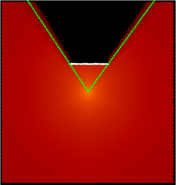
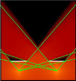
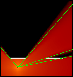
Figure 5: Photon density maps of 2D shadowing tests in three different cases: single point source with a single obstacle (left panel), two point sources with two obstacles (middle panel), and a single source with two obstacles (right panel). The green lines indicate the geometric boundaries of the expected shadow regions, whereas the thick white lines mark the absorbing obstacles.

For the time integration of the radiative source terms, we employ implicit or semi-implicit methods, as described in Section 2.5, that are stable even for very large time steps, and in selected situations, adaptive numerical integration of the stiff ordinary differential equations that describe the chemical networks. The latter is essential to accurately account for non-equilibrium effects. As these processes are completely local, this does usually not incur a very significant computational cost, provided the exact integration is only done where really needed. In contrast, the timestepping of the radiation advection step poses more severe computational requirements. This is because this step is based on an explicit time integration scheme, whose timestep needs to obey a Courant criterion of the form

$$\Delta t_{\rm advect}<C_{k}\frac{\Delta x\,a}{c},$$ (31)

where $0<C_{k}<1$ is the Courant factor, and $\Delta x$ is taken to the smallest comoving size of a cell in the simulated volume.

In ordinary hydrodynamics, a similar time step constraint is encountered, except that the speed of light is replaced with the speed of sound. Since we are primarily interested in non-relativistic gas dynamics in cosmological structure formation, the speed of light will typically be a factor $\sim 10^{2}$ to $10^{4}$ larger than the hydrodynamical sound speed. The resulting reduction in the allowed time step size can hence make a simulation prohibitively expensive when the RT is coupled to the hydrodynamics over significant fractions of the Hubble time. However, in many applications of interest this problem can be greatly alleviated by resorting to an artificially reduced speed of light $c^{\prime}$, which is introduced instead of the physical speed of light both in the transport equation and the ionisation equation. As Gnedin & Abel (2001) and Aubert & Teyssier (2008) discuss in detail, this reduced speed-of-light approximation is especially attractive for cosmic reionisation problems because it here does not modify the propagation speed of I-fronts, except perhaps in the very near field region around a source directly after it turns on, but this introduces a negligible timing error. In general, the reduced speed-of-light approximation can be expected to yield reasonable accuracy in many radiation hydrodynamic problems as long as $c^{\prime}$ remains significant larger than the maximum sound speed occurring in the simulation.

2.8 Implementation aspects in the moving-mesh code AREPO

We have implemented the different variants of our radiation advection solver in the moving-mesh code AREPO (Springel, 2010). This code treats hydrodynamics with an ordinary finite-volume approach and a second order accurate Godunov scheme, similar to many Eulerian grid codes. However, AREPO works on an unstructured mesh created with a tessellation technique. The particular mesh used is the Voronoi tessellation created by a set of mesh-generating points. Using such a mesh offers a number of advantages compared to traditional grid codes in that its mesh can flow along with the gas. As a result of the induced dynamic mesh motion, AREPO exhibits considerably lower advection errors than ordinary mesh codes, and also avoids the introduction of preferred spatial directions. Also, the cell size automatically and continuously adjusts to the density in a Lagrangian sense, and is hence decreased in regions where typically more resolution is required even without doing adaptive mesh refinement.

For implementing our RT transfer scheme as described above, we can readily employ the infrastructure and communication algorithms provided by the fully parallelised AREPO code, making it an ideal base for a first demonstration of the method. This in particular applies to the gradient estimation, the spatial reconstruction of the photon intensity fields, and the parallelisation for distributed memory computers. A full description of these aspects of our code can hence be found in Springel (2010). We carry out a RT step on every top-level synchronisation point of the AREPO code, which means on the longest time step $\Delta t_{\rm max}$ allowed by the gravitational and hydrodynamical interactions followed by the code. If $\Delta t_{\rm advect}$ is smaller than the top-level simulation time-step $\Delta t_{\rm max}$, the radiation transfer step is calculated in several sub-cycling steps equal to or smaller than $\Delta t_{\rm advect}$, as needed.

Note that these sub-cycling steps do not require a new construction of the Voronoi mesh, or a new gravity calculation, hence they are in principle quite fast compared to a full step of the hydrodynamic code. However, this advantage can be quickly (over)compensated by the need to carry out multiple flux calculations for each of the angular components of the radiation field, and the additional need to do subcycling in time to ensure stability of the explicit time integration used in the advection steps. Furthermore, if a multiple frequency treatment is desired, the cost of the radiative transfer calculations will scale linearly with the number of frequency bins employed, simply because the dominating advection part of the radiative transfer problem needs to be carried out for each frequency independently. The additional storage requirements for a multiple frequency treatment should also not be overlooked, which again scale linearly with the number of frequency bins, likewise with the number of solid-angle bins used in the angular discretisation. It is hence clear that multi-frequency radiative transfer at high angular resolution clearly remains expensive with the discretisation scheme proposed here. However, the relative cost increase compared to hydrodynamics alone is a constant (and at least for sufficiently interesting problems still affordable) factor that is nearly independent of spatial resolution. This, together with the ability of our scheme to cope with essentially arbitrary source functions, makes it an interesting new technique for cosmological hydrodynamics.

3 Basic test problems

3.1 Shadows around isolated and multiple point sources

We begin our investigation of the accuracy of our proposed radiative transfer algorithms with isolated point sources in an optically thin medium that includes some regions with absorbing obstacles. This serves both as a verification that an isolated point source produces a radiation field $n_{\gamma}\propto 1/r^{2}$ (in 3D, and $n_{\gamma}\propto 1/r$ in 2D), with sufficiently spherical isophots, and as a test whether the method can cast sharp shadows behind obstacles. The latter is often difficult for RT transfer schemes, especially the ones that are diffusive in character such as the OTVET scheme (e.g. Gnedin & Abel, 2001; Petkova & Springel, 2009).

In Figure 5, we show such shadowing tests for three different cases, which for visualisation purposes have been done in 2D space. In the left hand panel, we consider the shadow that is produced by an obstacle when it is illuminated by a single source in the middle of the panel. The green lines show the geometric boundaries of the theoretically expected position of the shadow. We see that the obstacle produces a rather sharply defined shadow with only a small radiation leak into the shadowed region due to numerical advection and discretisation errors along the shadow boundaries. In the unshadowed regions, the radiation intensity falls of as $\propto 1/r$, as expected.

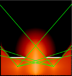
Figure 6: Radiation field around two point sources and two absorbing obstacles, for our hybrid treatment of point-sources and radiative diffusion. In this example, only the brightest source seen from a given cell was treated explicitly as a point source, while the other radiation was dumped into a background field transported with radiative diffusion.

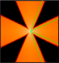
Figure 7: Illustration of our cone transport scheme, and the accuracy with which it can represent homogeneously illuminated radiation cones. The panel shows a map of the 2D photon density around a single source positioned at the center of the field. Radiation transport was calculated by partitioning the full $2\pi$ angle into eight regions of size $\pi/4$ each, with each of the fields transported individually. To show that the cones produce a homogeneous field, the source luminosity was only injected into every second cone and some of the cone boundaries were marked with green lines.

Equally good results are also obtained when multiple sources are considered in our “linear sum” approach to the total radiation field, where the total photon density is computed as a linear sum of the photon fields from each source, and the transport of each partial field is treated independently. Examples for this are shown in the middle and right panels of Figure 5, where two obstacles and one or two sources are used in different configurations. Again, the shadows agree very well with the expected boundaries shown with green lines, with only a small amount of residual diffusion into the shadowed regions. If the spatial mesh resolution is improved, the shadows become progressively sharper still.

We note that the above success essentially holds in this approach for an arbitrary set of absorbing regions, and an arbitrary combination of point sources. It hence provides a general and highly accurate solution to the radiative transfer problem, even though it can certainly get expensive to obtain it, especially for a large number of source. It is important to note however that the radiation fields produced by our scheme are essentially noise-free, which is a drastic improvement compared to results obtained from schemes that rely on Monte-Carlo methods (e.g. Maselli et al., 2003), or on randomised cone transport (Pawlik & Schaye, 2008).

As we discussed earlier, for many problems in astrophysics the number of sources is too large to make the linear sum approach a viable solution technique. In our first approach to work around this limitation, we only treat the photons from the brightest sources at a given cells as independent point sources in the transport scheme, while all other incoming photons form fainter sources are added to a background radiation field, which is then diffused from cell to cell. In Figure 6, we show a (somewhat extreme) example for how this can change the results. We repeat the test shown in the middle panel of Fig. 5, which has two sources and two obstacles, but this time we only allow the code to treat the locally brightest $N_{\rm br}=1$ sources as explicit point sources, while the rest of the radiation needs to treated with radiative diffusion. As we can see from Figure 6, the radiation field near to the two sources is unchanged, as expected, but at the mid-plane, where the sources have equal intensity, half of the flux is dumped into a diffusive reservoir. The diffusion approximation then lets the radiation spread from the mid-plane more slowly, causing an incorrect increase of the radiation intensity there. A second effect is that the shadows behind the obstacles are not sustained as nicely any more, instead they are partially illuminated by the radiative diffusion. It is important to be aware that unlike in the pure transport scheme considered earlier, these errors will not become smaller for an improved mesh resolution, rather, one would simply converge to a wrong solution in this case.

The example studied in Fig. 6 is deliberately extreme in the sense that $N_{\rm br}$ was kept very low. Much better results can be expected for a sizable value of $N_{\rm br}$, say $5-10$, because then the flux that needs to be treated with the diffusion approximation should become locally sub-dominant everywhere. Nevertheless, for general radiation fields and smoothly distributed source functions, we prefer our “cone transport” scheme, which we now begin to evaluate in the context of shadowing.

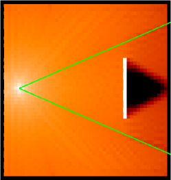
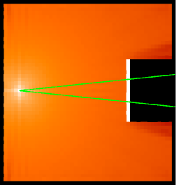
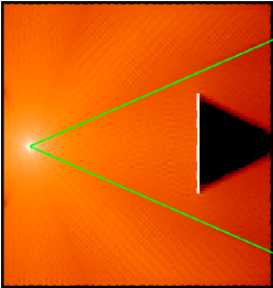
Figure 8: Maps of the photon density field obtained with our “cone transport” scheme for a point source at coordinates $(0.1,0.5)$ and an obstacle (shown in white) centered at coordinates $(0.72,0.5)$. The three panels differ in the mesh resolution used and the angular resolution employed for the radiation transfer. In all panels, the angular size of the cones employed in the angular discretisation are shown with green lines. In the left panel, where eight cones are used, the obstacle’s opening angle as seen from the source is smaller than the fundamental cone, and therefore no complete shadow is formed. In the middle panel, 32 cones are used instead, such that the obstacle’s opening angle is now larger than the angular resolution, allowing a full shadow to be formed. Finally, in the right hand panel, the spatial mesh resolution has been doubled in each dimension compared to the panel on the left, while the number of angular resolution elements has been kept at eight. Again there is no complete shadow formed, as expected, but the boundary of the shadow region behind the obstacle is now more sharply defined.

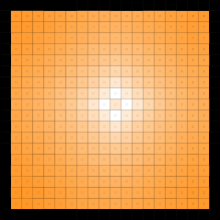
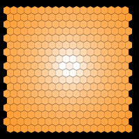
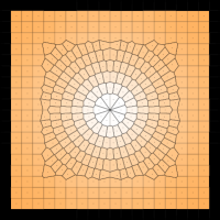
Figure 9: Maps of the photon distribution for 2D simulations with three different cell shapes: Cartesian square, hexagonal and azimuthal/unstructured. The line plot on the right shows the photon intensity profile, overplotted with the expected $r^{-1}$ law. The vertical line indicates the average cell size. Results from all mesh shapes agree well with the analytical prediction (dot-dashed line).

In Figure 7, we illustrate the ability of this transport scheme to produce homogeneously illuminated radiation cones with an opening angle equal to the angular resolution adopted for the scheme. In this example, a single source was placed in the center of a 2D unit square, and angular space has been divided into eight equal sized regions, with the source radiation only injected into four of them, alternating between an “empty” and a “full” cone. The green lines in the plot show some of the geometric boundaries of the angular discretisation as seen from the source. We see that the cone transport succeeds in producing a flat intensity profile as a function of angle within every illuminated cone, while at the same time the leaking of radiation into cones that should remain dark as seen from the source is very small. We note that if we let the source inject radiation into two adjacent cones with equal luminosity, the radiation field shows no trace of the angular boundary between the cones, thanks to our use of the total intensity field in calculating the local advection direction for the radiation of each partial field.

An interesting question now arises how this transport scheme deals with obstacles and the problem of shadowing. We illustrate the salient points with a few tests in Figure 8. Here, we illuminate an obstacle (shown in white) by a single source in the left part of the simulated 2D space. We vary both the angular and the spatial mesh resolution in order to study how the shadowing performs in the cone transport scheme. In the left panel, we have used $50^{2}$ cell and eight angular regions. The fundamental cone size is shown by the green lines. In this setup, the opening angle of the obstacle as seen from the source is hence smaller than the angular resolution of the RT, making the obstacle “unresolved”. In this case, the obstacle absorbs the correct amount of radiation expected for its size, but it will not form a correct shadow behind it. Instead, the “downstream region” behind the obstacle will get refilled with photons. As this can happen only by photons transported within the same geometric cone, a partial shadow is formed behind the object, with boundaries that are in principle parallel to the cone boundaries. In the middle panel, we repeat the test with the same spatial mesh resolution, but we have increased the number of cones to 32. In this way the angular size of the obstacle as seen from the source becomes larger than the angular resolution, allowing it to be resolved. As a result, a complete shadow is being formed, but this shadow is in general a bit smaller than the correct geometric shadow, with the difference being filled by a partial shadow, created in the cones that are only partially obscured by the obstacle. Finally, in the right hand panel, we have repeated the test on the left a second time, but now doubling the spatial resolution to $100^{2}$ cells while the angular resolution was kept unchanged. The primary difference this makes is that the borders of the partial shadow that is formed are now more sharply defined compared to the case with lower spatial resolution, as expected.

Finally, we examine how well our transport scheme can cope with different mesh geometries, which naturally arise in simulations with the AREPO code. In Figure 9 we show the radiation fields developing around a point source embedded in different mesh geometries: a Cartesian mesh, a hexagonal mesh (which is akin to the mesh geometry developing in AREPO in regions of constant resolution), and an azimuthal/unstructured mesh. For all four cases, we compare the created radiation fields to the expected profile in 2D, obtaining good agreement. This confirms the ability of our approach to work well with the unstructured Voronoi meshes produced by the AREPO code.

3.2 Isothermal ionised sphere expansion

We now turn to a test of our basic radiation advection scheme that involves both sources and sinks. To this end, we perform an ionised sphere expansion test in three dimensions, which is arguably the most fundamental and important test relevant for cosmic reionisation codes.

The expansion of an ionisation front in a static, homogeneous and isothermal gas is the only problem in radiation hydrodynamics that has a known analytical solution and is therefore indeed the most widely used test for RT codes. We adopt a monochromatic source that steadily emits $\dot{N}_{\gamma}$ photons with energy $h\nu=13.6\,\rm eV$ per second into an initially neutral medium with constant gas density $n_{\rm H}$. Then the Strömgren radius at which the ionised sphere around the source reaches its maximum radius is defined as

$$r_{\rm S,0}=\left(\frac{3\dot{N}_{\gamma}}{4\pi\alpha_{\rm B}n_{\rm H}^{2}}\right)^{1/3},$$ (32)

where $\alpha_{\rm B}$ is the recombination coefficient. If we approximate the I-front is infinitely thin, i.e. features a discontinuity in the ionisation fraction, then the temporal expansion of the Strömgren radius can be solved analytically in closed form, with the I-front radius $r_{\rm I,0}$ given by

$$r_{\rm I,0}=r_{\rm S,0}[1-\exp(-t/t_{\rm rec})]^{1/3},$$ (33)

where

$$t_{\rm rec}=\frac{1}{n_{\rm H}\alpha_{\rm B}}$$ (34)

is the recombination time and $\alpha_{\rm B}$ is the recombination coefficient.

More accurately, the neutral and ionised fraction as a function of radius of the Strömgren sphere can be calculated analytically (e.g. Osterbrock & Ferland, 2006) from the equation

$$\frac{\tilde{n}_{\rm HI}(r)}{4\pi r^{2}}\int{\rm d}\nu\,\dot{N_{\gamma}}(\nu)\,e^{-\tau_{\nu}(r)}\,\sigma_{\nu}\,=\,\tilde{n}_{\rm HII}^{2}(r)\,n_{\rm H}\,\alpha_{\rm B},$$ (35)

where $\tilde{n}_{\rm HI}$ is the neutral fraction, $\tilde{n}_{\rm HII}$ is the ionised fraction and

$$\tau_{\nu}(r)\,=\,n_{\rm H}\,\sigma_{\nu}\,\int_{0}^{r}{\rm d}r^{\prime}\,\tilde{n}_{\rm HI}(r^{\prime}).$$ (36)

Moreover, we can analytically solve for the radial profile of the photon density $n_{\gamma}(r)$, yielding

$$n_{\gamma}(r)=\frac{1}{c}\frac{\dot{N}_{\gamma}}{4\pi r^{2}}\,{\rm exp}\left\{-\int_{0}^{r}\kappa(r^{\prime})\,{\rm d}r^{\prime}\right\}.$$ (37)

From this we can also obtain the profile of the ionised fraction $\tilde{n}_{\rm HII}(r)$ as a function of time. We note that the Strömgren radius obtained by direct integration of equation (35) differs from the approximate expression (32) because it does not approximate the ionised region as a top-hat sphere with constant ionised fraction.

For definiteness, we follow in our tests the expansion of the ionised region around a source that emits $\dot{N}_{\gamma}=5\times 10^{48}\,{\rm s}^{-1}$ photons. The surrounding hydrogen number density is set to $n_{\rm H}=10^{-3}\,\rm cm^{-3}$ at a temperature of $T=10^{4}\,\rm K$. At this adopted temperature, the case B recombination coefficient is $\alpha_{\rm B}=2.59\times 10^{-13}\,\rm cm^{3}\,s^{-1}$. Given these parameters, the recombination time is $t_{\rm rec}=125.127\,\rm Myr$ and the expected Strömgren radius is $r_{\rm S,0}=5.38\,\rm kpc$.

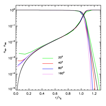
Figure 10: Profiles of the neutral and ionised fraction at the end of the ionised bubble expansion test, when the Strömgren radius $r_{\rm S,0}$ has been reached. The black line is the analytic solution based on equation (35), while the coloured lines are the numerical results for mesh resolutions of $20^{3}$, $40^{3}$, $80^{3}$, and $160^{3}$ cells, as labelled.

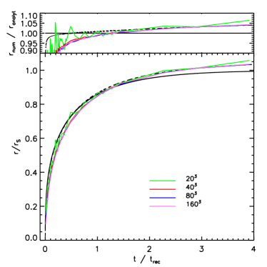
Figure 11: Radius of the ionised region as a function of time, in units of the recombination time $t_{\rm rec}$. The solid black line is the analytic solution from equation (35), while the dashed black line gives the simple approximation of equation (33). The coloured lines give our numerical results for different mesh resolutions equal to $20^{3}$, $40^{3}$, $80^{3}$, and $160^{3}$ cells. We see that the ionising front is slower than the theoretical prediction in the beginning of the expansion, as a result of the artificially reduced speed of light adopted here. At late times, the numerical result agrees however very well with the analytical solution.

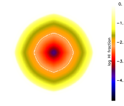
Figure 12: Map of the neutral fraction in a slice through the center of our Strömgren sphere test (based on our point-source advection scheme), for our highest resolution simulation with $160^{3}$ mesh cells. The white line shows the contour at a neutral fraction of 0.5.

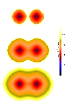
Figure 13: Neutral fraction in a slice through the center of two nearby sources of equal luminosity that ionise neutral gas. The three panels from top to bottom show different evolutionary stages. The top panel shows a stage before the ionised spheres overlap ($t=25\,\rm Myr$). Here they have exactly the same shape and do not influence each other yet. In the middle panel, the two have begun to overlap ($t=100\,\rm Myr$), while in the bottom panel the final state is shown, where the ionised region becomes time invariant ($t=500\,\rm Myr$).

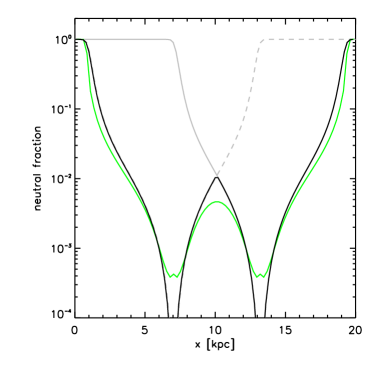
Figure 14: Neutral fraction along a line passing through the centres of two nearby sources that ionise the background gas. The green line shows the numerical result, whereas the black lines are a simple composite model for the expected structure of the solution based on superposing the analytic solution for each of the sources (gray dashed line for the left source and gray solid line for the right source). This superposition of the individual sources describes the numerical solution reasonably accurately, but we note that it is not the correct solution; the latter can only be obtained numerically for this problem.

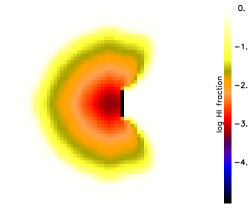
Figure 15: Map of the neutral fraction in a slice through the center of a Strömgren sphere. Unlike in our previous tests, an absorbing obstacle in the form of an optically thick disk was included as well (shown as a black line). We find that a nice shadow is produced behind the disk, with the inobscured directions developing as in the Strömgren sphere without an obstacle.

In Figure 10, we show the profiles of ionised and neutral fraction at the end of the ionised sphere expansion, when the Strömgren radius has been reached. We present results for simulations with four different spatial resolutions, using grids with $20^{3}$, $40^{3}$, $80^{3}$ and $160^{3}$ cells, respectively, using our point-source advection scheme. The results for all resolutions agree well with the analytical solution. The largest errors occur close to the central point source, but with better spatial resolution they become progressively smaller. In Figure 11, we show the time evolution of the ionising front, for the same simulations. The position of the front is determined as the distance from the source at which the ionised fraction equals $0.5$. The agreement with the analytical solution is generally good and improves with better resolution. However, in the beginning, the ionisation front moves noticeably slower than expected, which is due to our use of the reduced speed of light approximation with $c^{\prime}=c/1000$. At later times, this initial error becomes unimportant, however, and the numerical solution matches the analytic expectation well. Making the start-up error vanishingly small would be possible, if desired, but requires using $c^{\prime}=c$.

In Figure 12, we show a map of the neutral fraction in a slice through the source plane for the resolution $160^{3}$. We notice that the isophotal shapes exhibit small departures from a perfectly spherical shape, which originate in spatial discretisation errors close to the source. In fact, these deviations depend on the geometry of the source cell itself. For a hexagonal mesh structure as it occurs for a regularised Voronoi mesh in 2D dimensions, the errors are noticeably smaller than for the Cartesian mesh employed here. Higher spatial resolution alone will normally not be able to decrease the deviations to arbitrarily small levels, but spreading the point source over multiple cells (effectively resolving the source geometry) can make the isophots perfectly round if desired. We note that our cone transport scheme also does a good job in producing round isophots, even when a single cell is used as source.

As a simple variant of the isolated source case, we have also considered the evolution of the ionised regions around two sources that are $4\,\rm kpc$ apart, using our multiple point-source scheme. The density of the gas and the luminosity of each source are the same as in the previous test. In Figure 13, we show maps of the neutral fraction in a slice through the source at three different times: $t=25\,\rm Myr$ (top), $t=100\,\rm Myr$ (middle), and $t=500\,\rm Myr$ (bottom). An important point of this test is that the proximity of the sources does not affect the shape of the ionised regions at all until they begin to overlap. This is very different in the OTVET scheme, for example, where the early expansion is distorted because the Eddington tensor estimates already “feel” nearby sources even though they may still be completely hidden in their own ionisation bubbles. In Figure 14, we show the neutral fraction along a line passing through both sources at the final time. A simple model for the expected neutral fraction based on the superposition of the analytic single source solution is shown in black, while the numerical solution is shown in green. While the superposition model does a reasonably good job in describing the numerical solution, we note that the latter is showing important differences, for example for the radiation intensity between the sources. Our method allows an accurate calculation of this quantity, and similarly for more complicated setups.

In Figure 15 we show a further map of the neutral fraction in a slice through the source plane in a simple single-source Strömgren test. However, in this test we included an obstacle in the form of an optically-thick three dimensional plate, located $2\,\rm kpc$ from the source (shown in black in the figure). The setup is meant to test shadowing in 3D for a problem with non-trivial source function, and is designed to match the parameters of an equivalent test in Pawlik & Schaye (2008). We can see that our obstacle produces a clear shadow that remains fully neutral, as expected. Comparing our result to those of Pawlik & Schaye (2008, see their Fig. 10), we find good qualitative agreement but much reduced numerical noise.

Finally, we check whether using the cone transport scheme described in Section 2.4 is equally well capable of accurately solving the Strömgren sphere problem. To this end we have repeated our standard setup for the ionised sphere expansion of a single source, but this time employing direct discretisation of angular space using 12 cones for the full $4\pi$ solid angle, and a spatial mesh resolution of $40^{3}$. In the top and bottom panels of Figure 16 we show the profiles of ionised and neutral fraction at the end of the ionised sphere expansion, and the temporal evolution of the ionising front, respectively. The numerical results agree well with the analytical solutions, with an overall accuracy that is comparable to that of our point source treatment.

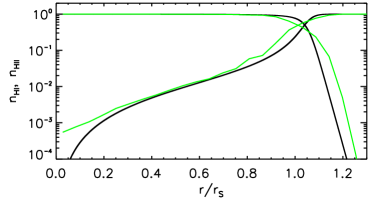
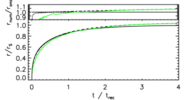
Figure 16: Strömgren sphere test for our ‘cone transport’ scheme where the angular space is decomposed into cones of equal solid angle. The panel on top shows the profiles of ionised and neutral fractions (green lines) versus distance from the source, in units of the Strömgren radius $r_{\rm S,0}$ at the end of the expansion at $t=500\,\rm Myr$. The analytical solution is given by the solid black line. The bottom panel shows the ionisation front radius as a function of time, relative to the Strömgren radius $r_{\rm S,0}$ as a function of time in units of the recombination time $t_{\rm rec}$. The numerical solution is shown in green and the analytical one in black.

3.3 Ionising front trapping in a dense clump

In our next test, we study the behavior of the code in a more challenging setting taken from the RT code comparison study of Iliev et al. (2006). A plane-parallel front of ionising radiation is incident on a dense, cold clump. The I-front penetrates the clump, ionises it and heats it up. Eventually, the I-front gets trapped half-way through the clump, and as the it is stopped inside the obstacle, a shadow is produced behind the clump.

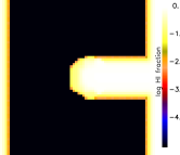
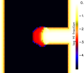
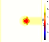
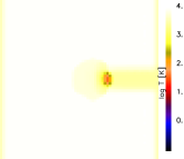
Figure 17: Maps of neutral fraction (top row) and temperature (bottom row), in a simulation of the interaction of a plane-parallel ionisation front with a dense clump. The two columns show our simulation results at two different times, $t=1\,\rm Myr$ (left) and $t=15\,{\rm Myr}$ (right). We note that already at the earlier time the background gas has been fully ionised. The I-front gets however stuck in the clump, producing a shadow behind it.

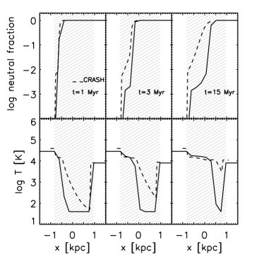
Figure 18: Neutral fraction and temperature as a function of distance from the center of the dense clump, at three different times: $t=1\,\rm Myr$ (left column), $3\,{\rm Myr}$ (middle) and $15\,{\rm Myr}$ (right). The shaded area shows the geometric extension of the clump. Results obtained with the code CRASH in the RT code comparison project are also included and shown as dashed lines.

Figure 19: Time evolution of the temperature, neutral fraction, and ionised front (solid lines) in the dense clump that is ionised by an impinging I-front. We also include results obtained with the code CRASH in the RT code comparison project, which are shown as dashed lines for comparison.

Our set-up of this test problem is as follows. We simulate a plane-parallel I-front with flux $F_{\gamma}=10^{6}\,\rm photons\,s^{-1}\,cm^{-2}$ that is incident on a dense clump, located $5\,\rm kpc$ away from the edge of the simulation domain. The ambient background gas has density $n_{\rm H}=2\times 10^{-4}\,\rm cm^{-3}$ and temperature $T=8000\,{\rm K}$. The radius of the clump is $r_{\rm clump}=0.8\,\rm kpc$, with a density of $n^{\rm clump}_{\rm H}=200\,n_{\rm H}$, and a temperature $T_{\rm clump}=40\,{\rm K}$. We note that in this test, following Iliev et al. (2006), the gas is not allowed to move due to pressure or gravitational forces, hence only radiative transfer is tested. The system is evolved for a period of $15\,\rm Myr$ with a resolution of $40^{3}$ cells. In Figure 17, we show the neutral fraction and the temperature of the system in slices through the centre of the clump at times $t=1\,{\rm Myr}$, and $15\,{\rm Myr}$. The I-front approaches from the left, moving to the right. At time $t=1\,\rm Myr$, already the whole box has been swept up by the ionising photons, with the clump producing a clear shadow in the downstream direction on the right hand side of the clump. As time advances further, the clump becomes more ionised and continues to heat up, but the shadow is preserved throughout the simulated time span without being filled in by diffusion.

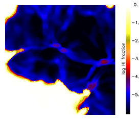
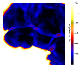
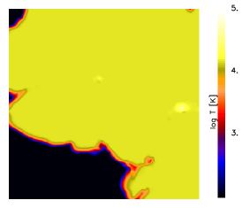
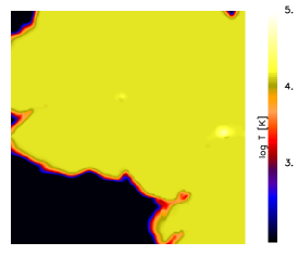
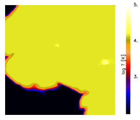
Figure 20: Maps of the ionised fraction (top row) and temperature (bottom row) in a slice through the middle of the simulation volume at time $t=0.4\,\rm Myr$ of our cosmological density field ionisation test. In the results shown in the left column, all sources have been treated independently as point sources. In the middle column, only the locally four brightest sources have been considered independently, while the remaining luminosity has been treated with radiation diffusion. Finally, the results in the right column are based on our cone transport algorithm with a division of the full solid angle into 12 cones of equal size, corresponding to the coarsest HEALPIX resolution.

In Figure 18, we show the temperature and neutral fraction as a function of distance from the geometric clump center. The results are compared to those obtained in the comparison study of Iliev et al. (2006) for the Monte-Carlos transfer code CRASH. The position and shape of the ionising front agree well with the results from the CRASH code, both at times $t=1\,{\rm Myr}$ and $15\,{\rm Myr}$. The temperature profile shows, however, some differences. This discrepancy can be traced back to inaccuracies in CRASH, where lower energy photons penetrate into the gas ahead of the ionising front and heat it there.

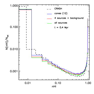
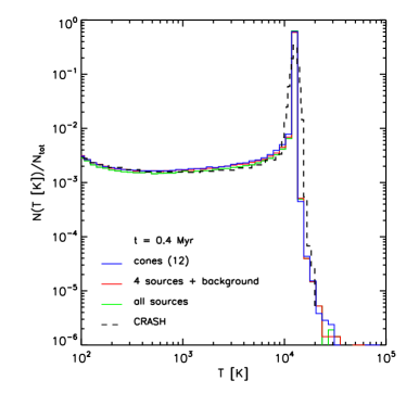
Figure 21: Distribution functions of the neutral fraction (top panel) and the temperature (bottom panel) in the simulated cosmological volume at time $t=0.4\,\rm Myr$, for three different variants of our radiation transfer scheme, as labelled: (1) all sources are followed in a linearly independent fashion, (2) only the four locally brightest sources are followed as point sources with the rest treated through radiative diffusion, and (3) a cone transport approach based on a division of the unit sphere into 12 cones. For comparison, we also include results obtained with the code CRASH in the RT code comparison project of Iliev et al. (2006).

Finally, in Figure 19 we show the time evolution of the temperature, ionised fraction and position of the I-front in the clump, compared to the results obtained with CRASH. The clump is 60% ionised at the end, its average temperature increases to several $10^{4}\rm K$ and the I-front becomes trapped around the geometric center of the clump, which is all in good agreement with the CRASH results. We hence conclude that our RT scheme yields results of good accuracy for this test, which are comparable in accuracy to those obtained with expensive yet accurate Monte-Carlo treatments.

3.4 Ionisation of a static cosmological density field

In our most demanding test of pure RT we follow hydrogen ionisation in a realistic cosmological density field, which is taken to be static for simplicity. Again, in order to be able to compare our results with those of the cosmological RT comparison project (Iliev et al., 2006) we use the same density field, the same cosmological box parameters, and assign sources in the same way. The test is based on a cosmological density field in a periodic box with size $0.5\,h^{-1}{\rm comoving\,Mpc}$ that resulted from the evolution of a standard $\Lambda$CDM model with the cosmological parameters $\Omega_{\rm 0}=0.27$, $\Omega_{\rm b}=0.043$, and $h=0.7$. The gas density field at redshift $z=9$ is considered for further analysis.

The source distribution is determined by finding halos within the simulation box with a Friend-Of-Friends (FOF) algorithm and then assigning sources to the $16$ most massive groups. The photon luminosity of these sources is taken to be

$$\dot{N}_{\gamma}=f_{\gamma}\frac{M\Omega_{\rm b}}{\Omega_{\rm 0}m_{\rm p}t_{\rm s}},$$ (38)

where $M$ is the total halo mass, $t_{\rm s}=3\,\rm Myr$ is the assumed lifetime of each source, $m_{\rm p}$ is the proton mass, and $f_{\gamma}=250$ is the number of emitted photons per atom during the lifetime of the source. For simplicity we also set the initial temperature of the gas to $100\,{\rm K}$ throughout the whole box.

Figure 22: Profiles of ionised fraction, hydrogen number density, pressure, temperature, and mach number at different times for a hydrodynamically coupled Strömgren sphere test. The distance from the source is normalised by the box size $L_{\rm box}=15\,\rm kpc$. The three lines in each plot correspond to the times $t=10\,\rm Myr$ (solid), $t=200\,\rm Myr$ (dashed), and $t=500\,\rm Myr$ (dotted).

In Figure 20, we show the neutral fraction and the temperature in slices through the center of the simulated volume, at the final evolution time of $t=0.4\,\rm Myr$. We have calculated the radiation transfer in three different ways, corresponding to the three variants of the radiation advection approach proposed in this paper. In the left panel, we show the results if all sources are treated as linearly independent point sources. The middle panel shows the result when only the $N_{\rm br}=4$ brightest sources seen from a given point are treated as point sources, while the remaining luminosity is fed to a background radiation field which is treated with radiative diffusion. Finally, the right hand panel gives the result when angular discretisation with 12 HEALPIX cones for the full solid angle is applied.

Visually, based on Fig. 20, all three results agree very well with each other. However, there are some small differences in the structure of the ionised regions and in the shape of the I-fronts. For a better quantitative comparison we show in the top panel of Figure 21 the volume filling function of the neutral fractions for all three simulation methods, where a comparison with CRASH results from the RT code comparison study (Iliev et al., 2006) is also included. Our results agree very well with the CRASH data, and we note that there are also no substantial differences between the three different approaches for dealing with multiple sources in our radiation advection scheme. The same conclusion is also reached from a comparison of the volume distribution function of the temperature, which is shown in the bottom panel of Figure 21. We note that these results are considerably better than those we obtained for the OTVET scheme implemented in the SPH code GADGET (Petkova & Springel, 2009).

3.5 Ionised sphere expansion in a dynamic density field

As our final test, we again follow the expansion of an ionised sphere in an initially homogeneous and isothermal medium, similar to Section 3.2, but this time we allow the gas to be heated up by the photons and to expand due to the raised pressure. This is hence a radiation hydrodynamics test where both RT and hydrodynamics are followed. We design our test similar to the set-up studied in Iliev et al. (2009). The source is at the center of the simulation domain and emits at a luminosity of $\dot{N}_{\gamma}=5\times 10^{48}\,{\rm s}^{-1}$ . The surrounding hydrogen number density is $n_{\rm H}=10^{-3}\,\rm cm^{-3}$ at an initial temperature of $T=10^{2}\,\rm K$. The simulated box is $30\,\rm kpc$ on a side, and is resolved with $160^{3}$ cells. We evolve the system for $500\,\rm Myr$.

There are two critical gas velocities defined for such a set up (Spitzer, 1978): the R-critical velocity $v_{\rm R}=2c_{\rm s}^{b}$ and the D-critical velocity $v_{\rm D}=c_{\rm s}^{b}-\sqrt{(c_{\rm s}^{b})^{2}-(c_{\rm s}^{a})^{2}}$, where $c_{\rm s}^{a}$ and $c_{\rm s}^{b}$ are the isothermal sound speeds ahead and behind the I-front, respectively. If we assume the ionised gas has temperature $10^{4}\,\rm K$ and the neutral gas $10^{2}\,\rm K$, than we obtain $v_{\rm R}\approx\rm 25.70\,km\,s^{-1}$ and $v_{\rm D}\approx 0.03\,\rm km\,s^{-1}$. The I-front is called D-type when its speed is smaller than the D-critical speed $v_{\rm I}\leq v_{\rm D}$. In this case it is subsonic with respect to the neutral gas, which expands as the I-front passes through it. When $v_{\rm I}\geq v_{\rm R}$, the I-front is called R-type. It is supersonic with respect to the neutral gas ahead, and the gas does not expand as the I-front passes trough it. When $v_{\rm D}<v_{\rm I}<v_{\rm R}$, there is a hydrodynamic shock wave in front of the I-front. The position of the I-front in this stage is given by (Spitzer, 1978)

$$r_{\rm I}=r_{\rm S,0}\left(1+\frac{7c_{\rm s}t}{4r_{\rm S,0}}\right),$$ (39)

where $c_{\rm s}$ is the sound speed of the ionised gas and $r_{\rm S,0}$ is the Strömgren radius given by equation (32).

Figure 23: Evolution of the position of the ionising front in a hydrodynamically coupled Strömgren sphere test. The distance is expressed in terms of the Strömgren radius $r_{\rm S,0}$ for the case of a static density field. The dotted line shows the analytic solution for the time evolution in the static density case, while the dashed line gives the solution for the dynamic density case. The latter is well reproduced by our numerical AREPO calculation. In the bottom panel, we show the speed of the ionisation front. In the first $40\,\rm Myr$ of the expansion, the front moves with a speed higher than the R-critical velocity (indicated by a dotted line).

We evolve our test setup for $500\,\rm Myr$ and analyse the results at three different times equal to $t=10,\,200$ and $500\,{\rm Myr}$. Figure 22 shows the time evolution of the profiles of the ionised fraction, hydrogen number density, pressure, temperature, and mach number profiles. At time $t=10\,\rm Myr$, the gas expands at subsonic speed. The pressure inside the ionised bubble is very high as the density is still relatively close to $10^{-3}\,\rm cm^{-3}$ and the temperature is several $10^{4}\,\rm K$. At later times, $t=200\,\rm Myr$, there is a shock developing ahead of the ionising front. The gas in this pseudo shock region is compressed, leading to densities higher than $10^{-3}\,\rm cm^{-3}$ and an increased pressure. At time $t=500\,\rm Myr$, the dynamic situation of the gas is similar, as there is still a shock ahead of the ionising front, but the pressure in the ionised bubble has dropped significantly due to the lowered density of the gas.

In Figure 23, we show the evolution of the radius of the I-front. In the first $40\,\rm Myr$, the ionising front moves with a speed larger than the R-critical velocity: $v_{\rm I}>v_{\rm R}$. Its evolution corresponds to that of an I-front in a static density field, and the position of the front follows the analytical prediction from equation (33). The gas does not expand significantly in this stage. As the speed of the I-front drops below the R-critical velocity, a shock develops ahead of it and the gas gets compressed in these regions. Here the position of the front evolves according to equation (39).

In general, our results for this test agree well with the other codes that have been tested by Iliev et al. (2009). We find the best agreement with the ENZO-RT results from the RT comparison study, which is probably due to the specific monochromatic nature of our code.

4 Discussion and Conclusions

In this study, we have proposed a novel implementation of radiative transfer and implemented it in the moving-mesh code AREPO. The method differs substantially from commonly employed ray-tracing or moment-based schemes in that it directly evolves a discretised version of the Boltzmann equation describing the photon distribution function. This is done in terms of an advection treatment, where the photon transport is carried out with a second-order accurate upwind scheme, based on methods that are commonly employed in hydrodynamic mesh codes. We have introduced three different approaches to deal with multiple sources, either by splitting up the radiation field into a linear sum of the partial fields created by all sources, by using a hybrid approach consisting of an exact treatment of the locally brightest sources combined with radiative diffusion, or by employing a direct discretisation of angular space into a finite set of cones. The latter approach is the most general. At a given angular resolution, it can easily deal with an arbitrary number of sources as well as with radiation scattering. Also, if the number of angular cones is enlarged, its angular accuracy becomes progressively better, allowing a simple way to test for convergence with angular resolution.

The radiation transport in our method is manifestly photon conserving. Combined with a photon-conserving treatment of the source terms, this yields a very robust description of the reionisation problem, ensuring that ionisation fronts propagate at the correct speed. If needed, our code can employ a reduced speed-of-light approximation that avoids overly small timesteps while not altering the growth of ionised regions in any significant way.

We have presented tests of our new scheme in a variety of cases. Using different photon transport tests in 2D, we have shown that our method manages to accurately capture shadows, and to produce the correct radiation fields independent of the mesh geometry. To test the coupling of gas physics with the photon transport we have carried out isothermal ionised sphere expansion tests and compared to the analytical solutions. The results agree reassuringly well with theoretical expectations, both for our linear summation method and the cone transport approach. Furthermore, we have shown that our method can treat multiple point sources in a highly accurate way, without the problem of a detrimental mutual influence of the sources onto each other, which is encountered in certain moment-based schemes (Gnedin & Abel, 2001; Petkova & Springel, 2009). We have also shown that our code performs well on the problem of the ionisation of a static cosmological density field, where we benchmarked our results against those obtained for the same setup in the radiative transfer comparison study of Iliev et al. (2006). Similarly, our results for I-front trapping in a dense clump, and for a hydrodynamically coupled Strömgren sphere agree well with those of other radiative transfer codes included in Iliev et al. (2006).

Compared to other radiative transfer schemes, our new method based on the cone transport features several interesting advantages. Unlike long-characteristics or Monte Carlo schemes, it avoids any strong sensitivity of the computational cost on the number of sources, and it does not concentrate the computational effort in regions close to the sources, which greatly helps in parallelising the calculations. Also, the ability to easily treat time-dependent effects that are consistently coupled to the hydrodynamic evolution is a substantial asset. Compared to moment-based solvers, our method can cast sharp shadows, and it performs accurately both in the optically thin and the optically thick regimes.

Our cone-transport scheme bears some superficial resembles to the TRAPHIC scheme of Pawlik & Schaye (2008). However, unlike their approach, we do not rely on stochastic Monte Carlo techniques. Instead, we work with an explicit spatial reconstruction of the radiation field and a fixed set of angular cones. As a result, our radiation field is essentially free of stochastic noise, which is a significant advantage compared to Monte Carlo approaches and offers much better convergence rate.

We hence think that our new method represents a promising treatment of radiative transfer in cosmological simulations. Its simple and general principles make it applicable in a wide variety of different problems in astrophysics. In particular, it should not only be useful for studying reionisation of the Universe, but also, for example, for studying star formation in molecular clouds, where ionising radiation creates pillars or neutral dense gas (e.g. Gritschneder et al., 2009). Also, our RT solver coupled to AREPO should allow self-consistent and more accurate treatments of radiative feedback effects in hydrodynamic simulations of star formation, something that we will study in forthcoming work.

References

- Abel et al. (1999) Abel T., Norman M. L., Madau P., 1999, ApJ, 523, 66
- Abel & Wandelt (2002) Abel T., Wandelt B. D., 2002, MNRAS, 330, L53
- Ahn & Shapiro (2007) Ahn K., Shapiro P. R., 2007, MNRAS, 375, 881
- Altay et al. (2008) Altay G., Croft R. A. C., Pelupessy I., 2008, MNRAS, 386, 1931
- Alvarez et al. (2006) Alvarez M. A., Bromm V., Shapiro P. R., 2006, ApJ, 639, 621
- Aubert & Teyssier (2008) Aubert D., Teyssier R., 2008, MNRAS, 387, 295
- Baek et al. (2009) Baek S., Di Matteo P., Semelin B., Combes F., Revaz Y., 2009, A&A, 495, 389
- Bolton et al. (2005) Bolton J. S., Haehnelt M. G., Viel M., Springel V., 2005, MNRAS, 357, 1178
- Cantalupo & Porciani (2010) Cantalupo S., Porciani C., 2010, ArXiv e-prints, 1009.1625
- Cen (2002) Cen R., 2002, ApJS, 141, 211
- Ciardi et al. (2001) Ciardi B., Ferrara A., Marri S., Raimondo G., 2001, MNRAS, 324, 381
- Finlator et al. (2009) Finlator K., Özel F., Davé R., 2009, MNRAS, 393, 1090
- Gnedin & Abel (2001) Gnedin N. Y., Abel T., 2001, New Astronomy, 6, 437
- Górski et al. (2005) Górski K. M., Hivon E., Banday A. J., Wandelt B. D., Hansen F. K., Reinecke M., Bartelmann M., 2005, ApJ, 622, 759
- Gritschneder et al. (2009) Gritschneder M., Naab T., Burkert A., Walch S., Heitsch F., Wetzstein M., 2009, MNRAS, 393, 21
- Gritschneder et al. (2009) Gritschneder M., Naab T., Walch S., Burkert A., Heitsch F., 2009, ApJL, 694, L26
- Hasegawa & Umemura (2010) Hasegawa K., Umemura M., 2010, MNRAS, 407, 2632
- Iliev et al. (2006) Iliev I. T., Ciardi B., Alvarez M. A., Maselli A., Ferrara A., Gnedin N. Y., Mellema . G., Nakamoto T., Norman M. L., Razoumov A. O., Rijkhorst E.-J., Ritzerveld J., Shapiro P. R., Sus a H., Umemura M., Whalen D. J., 2006, MNRAS, 371, 1057
- Iliev et al. (2009) Iliev I. T., et al., 2009, MNRAS, 400, 1283
- Katz et al. (1996) Katz N., Weinberg D. H., Hernquist L., 1996, ApJS, 105, 19
- Kunasz & Auer (1988) Kunasz P., Auer L. H., 1988, Journal of Quantitative Spectroscopy and Radiative Transfer, 39, 67
- Maselli et al. (2003) Maselli A., Ferrara A., Ciardi B., 2003, MNRAS, 345, 379
- Mellema et al. (2006) Mellema G., Iliev I. T., Alvarez M. A., Shapiro P. R., 2006, New Astronomy, 11, 374
- Mellema et al. (1998) Mellema G., Raga A. C., Canto J., Lundqvist P., Balick B., Steffen W., Noriega-Crespo A., 1998, A&A, 331, 335
- Mihalas & Weibel Mihalas (1984) Mihalas D., Weibel Mihalas B., 1984, Foundations of radiation hydrodynamics. New York: Oxford University Press, 1984
- Nakamoto et al. (2001) Nakamoto T., Umemura M., Susa H., 2001, MNRAS, 321, 593
- Nayakshin et al. (2009) Nayakshin S., Cha S., Hobbs A., 2009, MNRAS, 397, 1314
- Osterbrock & Ferland (2006) Osterbrock D. E., Ferland G. J., 2006, Astrophysics of gaseous nebulae and active galactic nuclei. Astrophysics of gaseous nebulae and active galactic nuclei, 2nd. ed. by D.E. Osterbrock and G.J. Ferland. Sausalito, CA: Uni versity Science Books, 2006
- Paardekooper et al. (2010) Paardekooper J., Kruip C. J. H., Icke V., 2010, A&A, 515, A79
- Pawlik & Schaye (2008) Pawlik A. H., Schaye J., 2008, MNRAS, 389, 651
- Petkova & Springel (2009) Petkova M., Springel V., 2009, MNRAS, 396, 1383
- Razoumov & Cardall (2005) Razoumov A. O., Cardall C. Y., 2005, MNRAS, 362, 1413
- Reynolds et al. (2009) Reynolds D. R., Hayes J. C., Paschos P., Norman M. L., 2009, Journal of Computational Physics, 228, 6833
- Rijkhorst et al. (2006) Rijkhorst E.-J., Plewa T., Dubey A., Mellema G., 2006, A&A, 452, 907
- Ritzerveld & Icke (2006) Ritzerveld J., Icke V., 2006, Phys Rev E, 74, 026704
- Shapiro et al. (2004) Shapiro P. R., Iliev I. T., Raga A. C., 2004, MNRAS, 348, 753
- Sokasian et al. (2001) Sokasian A., Abel T., Hernquist L. E., 2001, New Astronomy, 6, 359
- Spitzer (1978) Spitzer L., 1978, Physical processes in the interstellar medium. New York Wiley-Interscience
- Spitzer (1998) Spitzer L., 1998, Physical Processes in the Interstellar Medium. Wiley-VCH
- Springel (2010) Springel V., 2010, MNRAS, 401, 791
- Susa (2006) Susa H., 2006, PASJ, 58, 445
- Trac & Cen (2007) Trac H., Cen R., 2007, ApJ, 671, 1
- Whalen & Norman (2006) Whalen D., Norman M. L., 2006, ApJS, 162, 281
- Whitehouse et al. (2005) Whitehouse S. C., Bate M. R., Monaghan J. J., 2005, MNRAS, 364, 1367