Time operators in stroboscopic wavepacket basis and the time scales in tunneling

Abstract

We demonstrate that the time operator that measures the time of arrival of a quantum particle into chosen state can be defined as a self-adjoint quantum-mechanical operator using periodic boundary conditions on applied to wavefuncions in energy representation. The time becomes quantized into discreet eigenvalues and the eigenstates of the time operator, the stroboscopic wavepackets introduced recently [Phys. Rev. Lett. 101, 046402 (2008).] form orthogonal system of states. The formalism provides simple physical interpretation of the time-measurement process and direct construction of normalized, positive definite probability distribution for the quantized values of the arrival time. The average value of the time is equal to the phase time but in general depends on the choise of zero time eigenstate, whereas the uncertainity of the average is related to the traversal time and is independent of this choise. The general fromalism is applied to a particle tunneling through resonant tunneling barrier in 1D.

I Introduction

The concept of time operator in quantum mechanics is a difficult and confusing oneLandauer94 ; Hauge89 ; Muga00 . Heisenberg formulated the time-energy uncertainity principle already in the early days of quantum theory, indicating through analogy with the position-momentum uncertainty principle, that some time operator should exist. However, shortly after this, Pauli argued that no such self-adjoint operator can exist Pauli26 . Further development in scattering theory pursued the search for an estimates of time-scales associated with quantum processes, establishing the phase time, the time delay seen in the motion of the maximum of a wavepacket as the relevant quantity Wigner55 ; Ohmura64 . This, however, turned out to be unsatisfactory due to inherent ambiguity in the preparation of the wavepackets or identification of its maxima or other features. Several imaginative approaches, like the so called Larmor-clock time Rybachenko67 ; Buttiker83 ; Sokolovski93 ; McKinnon95 ; Hauge89 or the traversal time Keldysh65 ; Buttiker82 ; Landauer94 were suggested to identify the relevant time-scales. However, no final formulation of the problem has been established nor a consensus has been reached if such a formalism should exist. Nonetheless, the time-scale related to tunneling is an extremely useful concept for relevance of many-body effects in electronic transport through nanostructures. This has been analyzed in the pioneering work by Jonson Jonson80 ; Jonson89 where the time scale of tunneling was determined by the time scale of formation of the image charge, causing alteration of the effective tunneling barrier Binnig84 ; Quek07 . More generally, our ability to characterize the time-scales of transit or tunneling of an electron through a nanocontacts would be extremely helpful in understanding the importance of interactions in ab initio description of quantum transport Kurth10 ; Mera10 ; Vignale09 ; Myohanen08 ; Koentopp05 ; Sai05 ; Jung07 .

Independently of these physically motivated treatments, a important step forward in understanding the time operator, not as a self-adjoint operator but rather as a positively valued operator measure, has been done by Holevo Holevo78 . Independently, Kijowski Kijowski74 heuristically constructed a distribution of a time-of-arrival for a quantum particle. His work was later developed into the formulation of the construction of probability distribution of the arrival timeDelgado97 ; Leon00 ; Hegerfeldt04 ; Hegerfeldt10 . Most recently, even the problem of non self-adjointness of the time operator for a free quantum particle has been addressed by Galapon Galapon04 ; Galapon05 by introducing the confined time of arrival operator (CTAO) within finite space using specific boundary conditions in the real space.

In the present paper, we propose an alternative formalism, the use of periodic boundary conditions in the energy representation that leads to a family of self-adjoint time operators. In contrast to the CTAO, arbitrary scattering potentials can be considered from the start and the related issue of normalization of the probability distribution for times Leon00 ; Hegerfeldt04 is also resolved. The boundary conditions in the energy representation lead to formal quantization of the time, similarly to the situation with the CTAO. The quantization of time is a useful mathematical tool for drawing a simple physical picture of the time-dynamics of the quantum particle within the orthogonal time-eigenstate basis. This is used for physical interpretation of the zero-time eigenstate and its relation to the conventional arrival-time operator Muga00 and the ’time-of-presence’ operator Holevo78 . However, within the energy representation, the formalism is similar to many previous uses of the time-operators in the form of diferentiation by energy Ohmura64 ; Holevo78 ; Pacher05 ; Torres-Vega07 ; Ordonez09 ; Olkhovsky09 . Our formalism is demonstrated on a simple example of scattering of a particle on a resonant potential in 1D.

II Definition and general proparties of the time operator

In our work we will consider a quantum particle moving along x axis, characterized by its Hamiltonian $\hat{H}$ assumed to have continuous spectrum, occupying a state $\left|\phi\right\rangle$. For this particle we introduce a family of time operators, $\hat{\tau}_{\eta}$, where each of them gives the time it took for the particle to arrive into the state $\left|\phi\right\rangle$, assuming its dynamics has been governed by $\hat{H}$. The concept of the time operator also demands a definition of the zero of the time for certain state, which will be discussed after the operator is introduced. Different zero-time states are in one-to-one correspondence to different members of the family of time operators.

For the state $\left|\phi\right\rangle$, we will assume that it can be expressed as a linear combination of the Hamiltonian eigenstates, $\left|\epsilon,\alpha\right\rangle$, with energies from a finite interval, the energy band $\epsilon\in(\epsilon_{0},\epsilon_{0}+\Delta\epsilon)$,

$$\left|\phi\right\rangle=\sum_{\alpha}\int_{\epsilon_{0}}^{\epsilon_{0}+\Delta\epsilon}d\epsilon g_{\phi}(\epsilon,\alpha)\left|\epsilon,\alpha\right\rangle,$$ (1)

where $\alpha$ is the quantum number for degenerate states at the energy $\epsilon$. This degeneracy arises from some other operator $\hat{A}$ (or possibly several operators) that commutes with the Hamiltonian. The eigenstates are chosen so as to be common eigenstates of both $\hat{A}$ and $\hat{H}$. The complex amplitude $g_{\phi}(\epsilon,\alpha)$ represents the state $\left|\phi\right\rangle$ in the energy-band representation. The eigenstates are normalized to the delta function of energy, and the amplitude is normalized to one. This representation is not unique, another one can be obtained choosing a different operator $\hat{B}$ that also commutes with $\hat{H}$ (but not with $\hat{A}$). The representations are then related through an energy-dependent unitary transformation

$$\left|\epsilon,\alpha\right\rangle=\sum_{\beta}U_{\alpha,\beta}(\epsilon)\left|\epsilon,\beta\right\rangle.$$ (2)

We will assume that the amplitude for the state $\left|\phi\right\rangle$ has a support within the considered energy band so that at the ends of the interval we have $g_{\phi}(\epsilon_{0},\alpha)=g_{\phi}(\epsilon_{0}+\Delta\epsilon,\alpha)=0$. The states $g_{\phi}(\epsilon,\alpha)$ form a subspace of the Hilbert space $\mathcal{H}_{\Delta\epsilon}$ of all square-integrable states $g(\epsilon,\alpha)$ that are periodic within the energy band. Extending the width of the energy band, or considering a union of all energy bands covering the continuous spectrum of the Hamiltonian, and adding its possible bound states forms a complete set of states Bokes08 . However, for the purpose of introducing the time operators for state $\left|\phi\right\rangle$ it is sufficient to consider single energy band.

We will demonstrate that in the energy-band representation, within $\mathcal{H}_{\Delta\epsilon}$, the self-adjoint time operator can be defined as

$$\hat{\tau}_{\eta}=i\delta_{\alpha,\alpha^{\prime}}\frac{\partial~{}}{\partial\epsilon}+\eta_{\alpha,\alpha^{\prime}}(\epsilon).$$ (3)

Apart from the so-far unspecified Hermitian, energy-dependent matrix $\eta_{\alpha,\alpha^{\prime}}(\epsilon)$, and the fact that we define it only within the energy band, this operator has been known for long time as the operator for time in the energy-representation. It is well known that it is not self-adjoint if the whole spectrum is considered Holevo78 and not unique by the freedom of choice in the energy representation Hegerfeldt10 . The former is removed by the finite energy interval and the periodic boundary conditions employed. On the other hand, the freedom of choice of the energy representation in Eq. 1 is related to the choice of the Hermitian matrix $\eta_{\alpha,\alpha^{\prime}}(\epsilon)$ in the definition in Eq. 3. Using the unitary transformation, introduced in Eq. 2, $U_{\alpha,\beta}(\epsilon)=\exp\{i\int^{\epsilon}d\epsilon^{\prime}\nu_{\alpha,\beta}(\epsilon^{\prime})\}$ we find a transformed time operator

$$\hat{\tau}_{\eta^{\prime}}=i\delta_{\alpha,\alpha^{\prime}}\frac{\partial~{}}{\partial\epsilon}+\eta_{\alpha,\alpha^{\prime}}(\epsilon)-\nu_{\alpha,\alpha^{\prime}}(\epsilon).$$ (4)

Hence, starting from a particular energy-representation and a particular choice of $\eta_{\alpha,\alpha^{\prime}}(\epsilon)$, we can find a representation where the time operator is represented by the energy derivative only. This latter representation, if we had some rationale for choosing it independently of the time operator, could serve as the basis for definition of the time operator without any ambiguities.

The first step along this line is to demand that the time operator should commute with chosen operator(s) $\hat{A}$. Examples of these could be the linear or angular momentum, spin, etc. One of these is also the projector to the right- and left- going scattering states leading to $\alpha=R$ or $\alpha=L$ in 1D scattering that will be used in the next section. This reduces the matrix $\eta_{\alpha,\alpha^{\prime}}(\epsilon)$ into diagonal form and specifies the time operator for a processes which conserve the particular quantum number $\alpha$. For the simplicity of notation, we will not indicate this fact with any additional index for the time operator $\hat{\tau}_{\eta}$.

Further specification of $\hat{\tau}_{\eta}$ is related to the choice of zero time state, as discussed below, but in general no unique definition of the time operator will be given. Instead, we will accept that we deal with a family of operators of the form given by Eq. 3 with $\eta_{\alpha,\alpha^{\prime}}(\epsilon)=\delta_{\alpha,\alpha^{\prime}}\eta_{\alpha}(\epsilon)$ and that for a specific calculations we need to choose one particular form.

The eigenfunctions of the time operator are

$$g_{\tau_{m},\alpha}(\epsilon,\alpha^{\prime})=\frac{1}{\sqrt{\Delta\epsilon}}e^{-i\tau_{m}\epsilon}e^{i\int^{\epsilon}d\epsilon^{\prime}\eta_{\alpha}(\epsilon^{\prime})}\delta_{\alpha,\alpha^{\prime}},$$ (5)

where

$$\tau_{m}=\frac{2\pi}{\Delta\epsilon}m,\quad m=0\pm 1,\ldots$$ (6)

are discreet eigenvalues of the time operator. Similarly to our finding, discreet eigenvalues were found in the construction of the confined time operator Galapon04 for a free quantum particle. In both cases, the quantization is nothing fundamental and arises only as a result of the choice of the energy band: the size of the time-quanta could be changed by simply changing the width of the energy band while the final average values of the time operator will remain independent of this choice, which becomes obvious when using the energy representation. Still, choosing a wider energy band, i.e. decreasing the quantum of time, is desirable if one is interested in finer details of the probability distribution in time variable.

Rewriting the time eigenstates from the energy-band representation into the abstract form we have

$$\left|\tau_{m},\alpha\right\rangle=\frac{1}{\sqrt{\Delta\epsilon}}\int_{\epsilon_{0}}^{\epsilon_{0}+\Delta\epsilon}d\epsilon e^{-i\tau_{m}\epsilon}e^{i\int^{\epsilon}d\epsilon^{\prime}\eta_{\alpha}(\epsilon^{\prime})}\left|\epsilon,\alpha\right\rangle.$$ (7)

This set of states is subspace of the stroboscopic wavepacket basis, recently introduced for the description of open non-equilibrium electronic systems Bokes08 ; Bokes09 . Here we see that it naturally arises as the set of eigenstates of the time operator defined on the chosen interval of energies.

The eigenstates with $m=0$, $\left|\tau_{0}=0,\alpha\right\rangle$, have eigenvalue of the time operator zero, i.e. this is the choice of the zero of time. Due to the unspecified phase $\eta_{\alpha}(\epsilon)$ there is a certain freedom in the choice of this zero time eigenstate (and hence a particular time operator). If a particle is in one of these states, it took zero time to arrive into it. On the other hand, for a state $\left|\tau_{m},\alpha\right\rangle$ it took it precisely the time $\tau_{m}=2\pi m/(\Delta\epsilon)$ for the particle to arrive there from $\left|\tau_{0},\alpha\right\rangle$, since from Eq. 7 we find

$$e^{-i\hat{H}\tau_{m}}\left|0,\alpha\right\rangle=\left|\tau_{m},\alpha\right\rangle.$$ (8)

Finally, for a particle in an arbitrary state within the energy band, $\left|\phi\right\rangle=\sum_{m,\alpha}c_{m,\alpha}\left|\tau_{m},\alpha\right\rangle$, and $|c_{m,\alpha}|^{2}=|\left\langle\tau_{m},\alpha|\phi\right\rangle|^{2}$ will be the probability for the particle to arrive into it in time $\tau_{m}=2\pi m/(\Delta\epsilon)$.

From the above it follows that the expectation value of the time $\tau^{\phi}_{\eta}$ in the state $\left|\phi\right\rangle$ is given by weighting the different time eigenvalues with the probabilities that the relevant eigenstate is present in the state $\left|\phi\right\rangle$,

$$\tau^{\phi}_{\eta}=\sum_{m,\alpha}|c_{m,\alpha}|^{2}\tau_{m}=\left\langle\phi\right|\hat{\tau}_{\eta}\left|\phi\right\rangle,$$ (9)

This is equivalent to using the form in Eq. 3 within the energy-band representation,

$$\tau_{\eta}^{\phi}=\sum_{\alpha}\int d\epsilon g^{*}_{\phi}(\epsilon,\alpha)\left[i\frac{\partial~{}}{\partial\epsilon}+\eta_{\alpha}(\epsilon)\right]g_{\phi}(\epsilon,\alpha).$$ (10)

which motivates the formal definition of the time operator by the Eq. 3. Clearly, the expectation value of the time operator depends on the choice of zero-time eigenstate, i.e. on the choice of the phases $\eta_{\alpha}(\epsilon)$. In contrast, for the uncertainty of this average,

$$\Delta\tau^{\phi}=\sqrt{\left\langle\phi\right|\hat{\tau}_{\eta}^{2}\left|\phi\right\rangle-(\left\langle\phi\right|\hat{\tau}_{\eta}\left|\phi\right\rangle)^{2}}$$ (11)

we find

$$\Delta\tau^{\phi}=\sum_{\alpha}\int d\epsilon\frac{\partial~{}}{\partial\epsilon}\left|g_{\phi}(\epsilon,\alpha)\right|^{2}$$ (12)

which is manifestly independent of the choice of the phases $\eta_{\alpha}(\epsilon)$ and hence characteristic of the whole family of time operators.

The whole family of time operators, Eq. 3, fulfills the canonical commutation relation with the Hamiltonian $\hat{H}=\epsilon\delta_{\alpha,\alpha^{\prime}}$, $[\hat{\tau},\hat{H}]=i$, if the latter is understood to act only on states $\left|\phi\right\rangle$ with finite support within the energy band. (A minor technical issue that can be dealt with arises if the whole $\mathcal{H}_{\Delta\epsilon}$ is considered, since there the Hamiltonian is not continuous at the boundaries of the energy band.) This commutation relation then leads automatically to the uncertainty relation for the mean square fluctuations in the energy and the time, $\Delta\tau\Delta H\geq 1/2$.

The argument due to Pauli Pauli26 ; Muga00 regarding the non-existence of the self-adjoint time-operator does not apply since the boundary conditions cause the energy-shift operator to move the states periodically within the band. Namely, using the orthogonality of the time-operators’ eigenstates (Eq. 5) we can expand the Hamiltonian’s eigenstates $\left|\epsilon,\alpha\right\rangle$, Eq. 7, into the former and find the identity

$$\hat{H}e^{-i\epsilon^{\prime}\hat{\tau}}\left|\epsilon,\alpha\right\rangle=\left[(\epsilon-\epsilon^{\prime})\textrm{mod}(\Delta\epsilon)\right]e^{-i\epsilon^{\prime}\hat{\tau}}\left|\epsilon,\alpha\right\rangle,$$ (13)

for $\epsilon\in(\epsilon_{0},\epsilon_{0}+\Delta\epsilon)$. On the other hand, if the periodic boundary conditions within the bands were not used, the above identity would not contain the modulo operation with the difference $(\epsilon-\epsilon^{\prime})$ and the result would be that the state $e^{-i\epsilon^{\prime}\hat{\tau}}\left|\epsilon,\alpha\right\rangle$ is an eigenstate of Hamiltonian with the eigenvalue $\epsilon-\epsilon^{\prime}$. Following Pauli, and in view of arbitrariness of $\epsilon^{\prime}$, this would be in contradiction with the existence of the lower bound on the eigenenergies. However, we have shown above that the use of the periodic boundary conditions removes this problem.

The here used time operator is, by its character, close to the ’time-of-presence’ mentioned in the review by Muga and Leavens Muga00 . However, many authors Kijowski74 ; Delgado97 ; Hegerfeldt04 ; Leon00 prefer the concept of the arrival-time operator that gives the average value of time for a quantum particle to arrive at a spatial position $x_{0}$ if initially (at time $t=0$) it was in a chosen state $\left|\psi\right\rangle$. One can easily see that such an operator is given by $-\hat{\tau}_{\eta}$, with a specific choice of the phases $\eta_{\alpha}(\epsilon)$. The latter is such that the zero-time eigenstates resembles the position eigenstate $\delta(x-x_{0})$ as much as possible. For example, for a free quantum particle the energy eigenstates are

$$\left\langle x|\epsilon,\alpha\right\rangle=\frac{1}{\sqrt{2\pi k}}e^{ikx},\quad k=\sqrt{2\epsilon},$$ (14)

and using the projection $\int d\epsilon\left|\epsilon,\alpha\right\rangle\left\langle\epsilon,\alpha|x_{0}\right\rangle$, one finds $\eta_{\alpha}(\epsilon)=(d/d\epsilon)\sqrt{2\epsilon}x_{0}$. The interpretation of this time operator is as follows: we expand the state $\left|\psi\right\rangle$ into the arrival-time operator eigenstates, $\left|\psi\right\rangle=\sum_{m}\left\langle\tau_{m},\alpha|\psi\right\rangle\left|\tau_{m},\alpha\right\rangle$. Then $|\left\langle\tau_{m},\alpha|\psi\right\rangle|^{2}$ is the probability that the particle in $\left|\psi\right\rangle$ will arrive into the $\left|\tau_{0}=0,\alpha\right\rangle$ in time $-\tau_{m}$. Identifying the zero-time eigenstate with measurement device at $x=x_{0}$ gives the sought Kijowski probability distribution Hegerfeldt04 ; Leon00 . However, we need to stress that the arrival state, i.e. the zero-time eigenstate, can be quite different from the position eigenstate $\delta(x-x_{0})$ so that it should not be interpreted literally as the probability of the time of arrival into $x_{0}$ exactly.

III Arrival time in tunneling problems

Figure 1: (color online) The form of the potential energy used for demonstration of the tunneling time scales in 1D. The potential has two delta-shaped barriers of strength $\lambda$ at its both ends and a constant value $u$ in between. Varying the latter gives access to various transport regimes - from resonant tunneling to opaque tunneling. The energy-band of the stroboscopic wavepacket representation is indicated with arrows.

We will now demonstrate the use of the time operator for calculation of the tunneling time scales involved in the dynamics of quantum particle in 1D. For the state into which we expect the particle to arrive we initially take a state $\left|\phi\right\rangle$, located on the right of the tunneling barrier and characterized by a momentum directed away from the barrier,

$$\left\langle x|\phi\right\rangle=\int_{\epsilon_{0}}^{\epsilon_{0}+\Delta\epsilon}\frac{d\epsilon}{\sqrt{2\pi k}}A_{\phi}(\epsilon)e^{ik(x-x_{R})},\quad x_{R}\gg 0,$$ (15)

where $x_{R}$ determines the average position of a particle in the state and $k=\sqrt{2\epsilon}$. The real amplitude $A_{\phi}(\epsilon)$ is a continuous, differentiable function with its support within the energy band. The time it takes for the particle to arrive into the state $\left|\phi\right\rangle$ from the left of the barrier will contain contribution of the time it took for the particle to tunnel.

The dynamics of the particle is governed by the Hamiltonian $\hat{H}$ which asymptotically, for $x\rightarrow\pm\infty$, is that of a free particle. Close to the origin there is non-zero potential energy $V(x)$. The Hamiltonian posses a continuous spectrum of doubly-degenerate energy-normalized right- and left- going eigenstates $\left\langle x|\psi_{\epsilon,R}\right\rangle$ and $\left\langle x|\psi_{\epsilon,L}\right\rangle$ of which we will explicitely need only the right-going ones,

$$\left\langle x|\psi_{\epsilon,R}\right\rangle=\psi_{\epsilon,R}(x)=\left\{\begin{array}[]{ll}\frac{e^{ikx}}{\sqrt{2\pi k}}+r(\epsilon)\frac{e^{-ikx}}{\sqrt{2\pi k}}&x<<0\\ t(\epsilon)\frac{e^{ikx}}{\sqrt{2\pi k}}&x>>0\end{array}\right.,$$ (16)

where $k=\sqrt{2\epsilon}$ and $r(\epsilon)$ and $t(\epsilon)$ are the reflexion and transmission amplitudes respectively.

As a illustrative example, we will consider the Hamiltonian $\hat{H}=(1/2)d^{2}/dx^{2}+V(x)$, where $V(x)=\lambda(\delta(x)+\delta(x-a))+(u/2)(1(x)-1(x-a))$ where $1(x)$ is the unit-step function, $\lambda=1$, $a=10.0$, and $v=0.1-0.65$ is a variable potential within the delta-functions (see Fig 1). As can be inferred from the amplitude and the phase of transmission amplitude shown in Fig. 2, these values offer variety of different transport regimes. It might be also interesting to mention that this Hamiltonian corresponds to a simple model of a perturbed monoatomic sodium chain Bokes09 . For the arrival state $\phi(x)$ in Eq. 15 we take $A(\epsilon)=N_{A}\left[\cos^{2}\left((\epsilon-\epsilon_{1})\pi/\epsilon_{2}\right)\right]$, where $\epsilon_{1}=\epsilon_{0}+\Delta\epsilon/2$ and $\epsilon_{2}=\Delta\epsilon$, with $\epsilon_{0}=0.2$ and $\Delta\epsilon=0.4$, which produces a convenient localized state covering the interesting features in the transmission and its phase (Fig. 2). The constant $N_{A}$ is fixed by the normalization of the state $\phi(x)$. The localization of the arrival state will be set at $x_{R}=100$ which for the chosen parameters will guarantee that its amplitude in the region of the nonzero potential is negligible.

We proceed by the selection of the time-operator. Firstly, the Hermitian matrix $\eta_{\alpha,\alpha^{\prime}}(\epsilon)=\eta_{\alpha}(\epsilon)\delta_{\alpha,\alpha^{\prime}}$ shall be diagonal in the basis of the scattering states so that $\alpha=R$ or $L$ for right- or left- going scattering states. Secondly, the phases of this matrix will form the zero-time eigenstate from the incoming scattering states at some initial time $T_{0}$,

$$\eta_{R/L}(\epsilon)=-T_{0}.$$ (17)

If $T_{0}$ were $<<0$, the zero-time eigenstates would look just like wavepackets formed from incoming plane-waves, localized far to the left (right) of the barrier for $\alpha=R$ ($L$) respectively. However, this only shifts its origin for the time, so that in our calculations we will simply use $T_{0}=0$.

Figure 2: (color online) The amplitude and the phase of the transmission amplitude $t(\epsilon)$ for a scattering state in the potential given in Fig. 1 for $u=0.3$ (upper panel) and $u=0.65$ (lower panel). Since the energy band consists of energies $\epsilon\in(0.2,0.6)$, the smaller $u$ corresponds to resonant transport where as the larger $u$ gives dominantly opaque tunneling regime.

To evaluate the average time of arrival into $\left|\phi\right\rangle$, we need to express this state in the energy representation of the above scattering states,

$$\left|\phi\right\rangle=\sum_{\alpha}\int d\epsilon\left|\psi_{\epsilon,\alpha}\right\rangle\left\langle\psi_{\epsilon,\alpha}|\phi\right\rangle,\quad\alpha=R,L$$ (18)

For the chosen state $\left|\phi\right\rangle$, Eq. 15, both $\left\langle\psi_{\epsilon,R}|\phi\right\rangle$ and $\left\langle\psi_{\epsilon,L}|\phi\right\rangle$ will be nonzero. The presence of the left-going states goes against our intention to characterize the tunneling time scale. The physically relevant state in which the time average should be calculated should consists of the right-going states only.

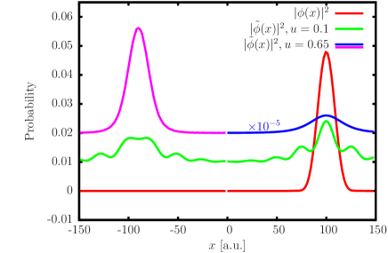
Figure 3: (color online) Probability densities of projected states $\tilde{\phi}(x)$ for $x_{R}=100$ into which the particle arrives, for two different potential barriers $u$. In contrast with the unprojected state $\phi(x)$, the arrival states are distorted and contain significant weight on both sides off the potential barrier (the amplitude for the state for $u=0.65$ on the right is $10^{5}$ times magnified so that it is visible) localized within $x\in(0,10)$.

To construct the final state correctly for a particle moving from the left to the right of the barrier, we need to construct a state $\left|\tilde{\phi}\right\rangle$, obtained from the state $\left|\phi\right\rangle$ by a von Neumann projection on the right-going states only, $\int d\epsilon\left|\psi_{\epsilon,R}\right\rangle\left\langle\psi_{\epsilon,R}\right|$,

$$\left|\tilde{\phi}\right\rangle=\frac{1}{\sqrt{N}}\int d\epsilon\left|\psi_{\epsilon,R}\right\rangle\left\langle\psi_{\epsilon,R}|\phi\right\rangle,$$ (19)

where $N$ is the normalization constant,

$$N=\int d\epsilon|\left\langle\psi_{\epsilon,R}|\phi\right\rangle|^{2}.$$ (20)

The state $\left|\phi\right\rangle$ for $x_{R}=100$ is negligibly small in the region where the states $\psi_{R}(x)$ differ from their asymptotic form for $x>>0$ in Eq. 16, so that

$$\left\langle\psi_{\epsilon,R}|\phi\right\rangle=t^{*}(\epsilon)A_{\phi}(\epsilon)e^{-ikx_{R}},$$ (21)

and $N=\int d\epsilon|A(\epsilon)t(\epsilon)|^{2}=\langle T\rangle$ has the meaning of the average transmission probability of the particle from the left to the right. The unprojected $\phi(x)$ and the projected states $\tilde{\phi}(x)$ for two extremal values of the potential parameters $u$ are shown in Fig. 3. It should be noted, that unlike $\phi(x)$, the projected states are distorted and contain a non-zero amplitude of the reflected state on the left of the barrier. This is necessary to have the total probability of arriving into the projected state at any time being one.

According to the general treatment, the probability that the particle arrived into state $\left|\tilde{\phi}\right\rangle$ at time $\tau_{m}$ is

$$P_{m} = \left|\left\langle\tau_{m},R|\tilde{\phi}\right\rangle\right|^{2}$$ (22)

$$= \frac{1}{\langle T\rangle}\left|\int\frac{d\epsilon^{\prime}}{\sqrt{\Delta\epsilon}}A_{\phi}(\epsilon)t^{*}(\epsilon^{\prime})e^{i\left[(\tau_{m}+T_{0})\epsilon^{\prime}-kx_{R}\right]}\right|^{2}$$

which is positive definite and normalized to one. The example of several such probabilities obtained for our particular example is shown in Fig. 4. For the energy band above the potential between the barriers ($u=0.1,0.3$), the particle will bounce between the barriers, resulting in the probability density of the arrival time into state to the right of the potential with several local maxima, separated by a time it takes for the particle to traverse the distance between the barrier twice. On the other hand, for a particle within a energy band below the potential barrier, no particular structure is visible. Clearly, different potentials lead to different distributions for arrival times and only the full probability distribution gives a complete picture of the time scales involved in the dynamics. Still for many cases two measures are most useful – the average value and its uncertainty.

Figure 4: (color online) The probabilities of arrival into state $\tilde{\phi}(x)$ at time $\tau_{m}$ for different transport regimes. In resonant transport ($u=0.3$), due to good localization of the state we see several maxima giving multiple bounces between the delta-function barriers; increasing $u$ into tunneling regime we first see very broad distribution ($u=0.53$) with its width characterized by the Buttiker-Landauer time, evolving into relatively narrow saturated distribution arriving earlier than the free particle (the Hartman effect).

The average time of the particle to arrive into the state $\left|\tilde{\phi}\right\rangle$ is most easily calculated within the energy-band representation,

$$\tau_{\eta}^{\tilde{\phi}} = \frac{1}{\langle T\rangle}\int d\epsilon|A_{\phi}(\epsilon)t(\epsilon)|^{2}\left[\frac{d\theta}{d\epsilon}+\frac{x_{R}}{v_{g}}-T_{0}\right],$$ (23)

where $\theta(\epsilon)$ is the phase of the transmission amplitude $t(\epsilon)=|t(\epsilon)|e^{i\theta}$. The additive term proportional to the average position $x_{R}$ is the classical expression $x_{R}/v_{g}$, where $v_{g}=d\epsilon/dk$ is the group velocity of the particle outside of the barrier. The first term is the generalization of the phase time since for a state within a narrow in energy band ($\Delta\epsilon\rightarrow 0$), the average time equals the well known expression $d\theta(\epsilon)/d\epsilon$. The choice of the phases $\eta_{R}(\epsilon)=-T_{0}$ leads to a simple shift in the time, independent of the transmission or the Hamiltonian’s potential. Keeping this form one can compare average times for different scattering potentials $V(x)$, localized close to the origin. In general, however, the energy-dependent phase leads to nontrivial change in the average time. Simple, potential-independent shift is found only if this energy dependence is negligible, i.e. $(d/d\epsilon)\eta_{R}(\epsilon)\Delta\epsilon\ll\eta_{R}(\epsilon)$.

According to Eq. 12, the uncertainty of the average time is given by

$$(\Delta\tau)^{2}=\int\frac{d\epsilon}{\langle T\rangle}\left(|A_{\phi}(\epsilon)t(\epsilon)|^{\prime}\right)^{2}.$$ (24)

There are two limiting cases: (1) $(d/d\epsilon)A_{\phi}\gg(d/d\epsilon)|t|$ the uncertainty is dominated by the energy width of the state $\left|\tilde{\phi}\right\rangle$, $A_{\phi}(\epsilon)$, and it does not carry information about the time scale in the scattering, and (2) $(d/d\epsilon)A_{\phi}\ll(d/d\epsilon)|t|$ when the uncertainty is dominated by the time scale known previously as the traversal time Buttiker82 and identified Buttiker83 as one of the Larmor clock times, $\tau^{L}_{z}=|t|^{-1}(d/d\epsilon)|t|$. Most importantly, the traversal time dominates the uncertainty whenever the the energy of the state moves under the barrier and the transmission is principally given by $|t|\sim\exp\{-d\sqrt{2(u-\epsilon)}\}$, where $d$ is the barrier width and $u$ its heigh. In Russian literatures it has been known as the Keldysh timeKeldysh65 ; Yucel92 and is approximately given as $\Delta\tau\sim d/\kappa$ where $\kappa=\sqrt{2(u-\epsilon)}$ is the magnitude of the imaginary momentum under the barrier. Our result are also in agreement with the observations of Yucel and Andrei that this is the time scale that should appear in the energy-time uncertainty principle Yucel92 . The identification of the traversal time with the variance of probability density of the dwell time has been also found by Olkhovsky Olkhovsky09 .

The appearance of the huge uncertainty in time, $\Delta\tau$, due to presence of the average energy of the state just below the barrier is demonstrated in Fig. 4 for $u=0.53$, in the very long tail towards large times of arrival. This will have significant effect on the tunneling process itself if the particle could interact with some additional degree of freedom within the barrier. This explains the appearance of this time scale in interacting tunneling models Jonson80 ; Jonson89 ; Buttiker82 ; Yucel92 . On the other hand, increasing the potential barrier further, the uncertainty is dominated by the energy width of the state $\tilde{\phi}(x)$, and hence independent of $u$ (e.g. $u=0.55$ and $u=0.65$).

Similarly to the traversal time, one can find a close correspondence between the average of $\hat{\tau}_{\eta}^{2}$ and the Buttiker-Landauer time Landauer94 $\tau_{T}$, but this statement, as any expression involving the phase time, is valid only for a particular choice of the phases in the zero-time eigenstate. This, however, is less important in tunneling regime, where $\Delta\tau$ is the dominant contribution to the average value of $\hat{\tau}_{\eta}^{2}$.

In the conclusions, we have introduced a family of self-adjoint time operators into the framework of standard quantum mechanics using periodic boundary conditions used on the amplitudes within the energy-band representation. This representation leads to quantization of time which is a useful tool to regularize the time-eigenstates and to draw physical interpretation of the use of this operator. We have shown that each member of the family of time operators fulfills the canonical commutation relation with the particle’s Hamiltonian and hence the energy-time uncertainty principle, identified its eigenstates are stroboscopic wavepackets, and showed how the present treatment avoids Pauli’s argument. In the context of the tunneling of a quantum particle, we have shown how a positively defined distribution function of times of arrival into an arbitrary state is obtained. Using the latter we have obtained the average value of the time operator which corresponds to the phase time which, however, is specific to a particular choice of the zero-time eigenstate and hence the particular choice of the time operator. In contrast, its uncertainty is independent of this choice and in the limit of narrow energy spread of the state it is equal to the traversal time scale of Buttiker and Landauer, or the Keldysh time. Our formalism confirms the role of energy derivative in energy representation as a legitimate time-operator in non-relativistic quantum mechanics and opens consistent ways for studding temporal behavior in many quantum-mechanical problems of interest.

The author wishes to acknowledge fruitful discussions with Martin Konôpka. This work was funded in part by the EU’s Sixth Framework Programme through the Nanoquanta Network of Excellence (NMP4-CT-2004-500198) and the Slovak grant agency VEGA (project No. 1/0452/09).

References

- (1) R. Landauer and T. Martin, Rev. Mod. Phys. 66, 217 (1994).
- (2) E. H. Hauge and J. A. Stovneng, Rev. Mod. Phys. 61, 917 (1989).
- (3) J. G. Muga and C. R. Leavens, Physics Reports 338, 353 (2000).
- (4) W. Pauli, in Handbuch der Physik, S. Fluegge, edited by S. Fluegge (Springer, Berlin, Germany, 1926), Vol. 5/1, p. 60.
- (5) E. P. Wigner, Phys. Rev. 98, 145 (1955).
- (6) T. Ohmura, Supp. of the Prog. Theor. Phys. 29, 108 (1964).
- (7) M. Büttiker, Phys. Rev. B 27, 6178 (1983).
- (8) D. Sokolovski and J. N. L. Connor, Phys. Rev. A 47, 4677 (1993).
- (9) V. F. Rybachenko, Sov. J. Nucl. Phys 5, 635 (1967).
- (10) W. R. McKinnon and C. R. Leavens, Phys. Rev. A 51, 2748 (1995).
- (11) M. Büttiker and R. Landauer, Phys. Rev. Lett. 49, 1739 (1982).
- (12) L. V. Keldysh, Zh. Eksp. Teor. Fiz. 47, 1945 (1965), [Sov. Phys. JETP 20, 1307 (1965)].
- (13) M. Jonson, Solid State Commun. 33, 743 (1980).
- (14) M. Jonson, Phys. Rev. B 39, 5925 (1989).
- (15) G. Binnig, N. García, H. Rohrer, J. M. Soler, and F. Flores, Phys. Rev. B 30, 4816 (1984).
- (16) S. Y. Quek, L. Venkataraman, H. J. Choi, S. G. Louie, M. S. Hybertsen, and J. B. Neaton, Nano Letters 7, 3477 (2007).
- (17) P. Myöhänen, A. Stan, G. Stefanucci, and R. van Leeuwen, Europhysics Lett. 84, 67001 (2008).
- (18) N. Sai, M. Zwolak, G. Vignale, and M. D. Ventra, Phys. Rev. Lett. 94, 186810 (2005).
- (19) J. Jung, P. Bokes, and R. W. Godby, Phys. Rev. Lett. 98, 259701 (2007).
- (20) S. Kurth, G. Stefanucci, E. Khosravi, C. Verdozzi, and E. K. U. Gross, Phys. Rev. Lett. 104, 236801 (2010).
- (21) H. Mera and Y. M. Niquet, Phys. Rev. Lett. 105, 216408 (2010).
- (22) G. Vignale and M. D. Ventra, Phys. Rev. B 79, 014201 (2009).
- (23) M. Koentopp, K. Burke, and F. Evers, Phys. Rev. B 73, 121403(R) (2006).
- (24) A. S. Holevo, Rep. Math. Phys. 13, 379 (1978).
- (25) J. Kijowski, Rep. Math. Phys. 6, 362 (1974).
- (26) J. León, J. Julve, P. Pitanga, and F. J. de Urríes, Phys. Rev. A 61, 062101 (2000).
- (27) G. C. Hegerfeldt, D. Seidel, J. G. Muga, and B. Navarro, Phys. Rev. A 70, 012110 (2004).
- (28) G. C. Hegerfeldt, J. G. Muga, and J. Muñoz, Phys. Rev. A 82, 012113 (2010).
- (29) V. Delgado and J. G. Muga, Phys. Rev. A 56, 3425 (1997).
- (30) E. A. Galapon, R. F. Caballar, and R. T. B. Jr, Phys. Rev. Lett. 93, 180406 (2004).
- (31) E. A. Galapon, F. Delgado, J. G. Muga, and I. n. Egusquiza, Phys. Rev. A 72, 042107 (2005).
- (32) V. S. Olkhovsky, Advances in Mathematical Physics 2009, 859710 (2009).
- (33) C. Pacher, W. Boxleitner, and E. Gornik, Phys. Rev. B 71, 125317 (2005).
- (34) G. Torres-Vega, Phys. Rev. A 75, 032112 (2007).
- (35) G. Ordonez and N. Hatano, Phys. Rev. A 79, 042102 (2009).
- (36) P. Bokes, F. Corsetti, and R. W. Godby, Phys. Rev. Lett. 101, 046402 (2008).
- (37) P. Bokes, Phys. Chem. Chem. Phys. 11, 4579 (2009).
- (38) S. Yücel and E. Y. Andrei, Phys. Rev. B 46, 2448 (1992).