Constraining String Gauge Field by Planet Perihelion Precession and Galaxy Rotation Curves

Abstract

We performed various tests on a cosmological model in which the string gauge field, and its coupling to matter, is used to explain the rotation dynamics of stars in a galaxy. Observations used include perihelion precession and galaxy rotation curves. We solved precession motions for perturbations of 1) a Lorenz-like force and 2) a general power law central force. For the latter case, a simple rule judging pro- or retrograde motions is derived. We attributed the precession of solar system planets to the force due to the string field and calculated the field strengths. We then fitted the resultant field strengths with a profile consisting one part generated by the Sun and another background due to other matter in the Milky Way. We used the Milky Way rotation curve to estimate the field strength and compared it with the one found by precession. The field strengths in another 22 galaxies are also analyzed. The strengths form a range that spans 2 orders of magnitude and contains the value found for the Milky Way. We also deduced from the model a relation between field strength, galaxy size and luminosity and verified it with data of the 22 galaxies.

1 Introduction

This is a paper analyzing a model proposed in CheungGRC0:2007 . The model is used as an alternative of dark matter to solve the galaxy rotation curve problem. It is conjectured that the gauge field in string theory provided the extra force needed to keep the rotation curves flat. Just like an electrically charge particle in magnetic field, the stringly charged matter in the string gauge field would also feel a force. In CheungGRC1:2008 , the string model was put into a contest with a particular dark matter model by fitting 22 galaxy rotation curves. These two models showed similiar fitting power. In this paper we further test this model with planet precessions in the solar system. In Iorio:2009 , possible anomalous precession for the Saturn was reported, and no explanation within convensional description of the solar system seems exist. It is thus interesting to ask if the effect of the string gauge field could explain the remaining anomalous precession. That serves as a test of the string model independent from that with rotation curves. For the consistency of the string model, it is also important to compare the field strength got by different methods and observations.

In section 2 we prepare the mathematics for precession analysis. Using Laplace-Runge-Lenz vector Goldstein:mechanics , we derive the precession rate formula for a magnetic like force. In addition, the case of power law central force is also analyzed and we find a simple precession formula, which is then tested in the Newtonian limit of Schwarzschild space-time and compared with other analysis on dark matter for the solar system.

In section 3 we attribute unexplained anomalous precessions to the magnetic like force in the string model. Using formulas derived, we use the precession data to find the string field strength in the solar system. The field strength is found to be on the order of $10^{-17}s^{-1}$ (with appropriate dimension, see below for the detail). Except at the Saturn, a decreasing pattern of the field strength with distances to the Sun is found. Other effects of the string field with that strength are also discussed.

The decreasing pattern of the field is further explored in the section 4. Assuming the string field in the solar system consists of one power law part from the Sun and a constant background from other matter in the Milky Way, a profile fitting of the field strength is done. The part from the Sun is found to go as $r^{-3}$, like a magnetic dipole. The background is found to be of opposite sign of the part from the Sun. This correctly matches with the fact that the rotation direction of the solar system is opposite to the one of the Milky Way.

To compare with the result from fitting precession, in section 5 we use the rotation curve of the Milky Way to estimate the field strength in the Milky Way. The connection of this result with the one from precession is then discussed.

In section 6 we first discuss the fitting result in CheungGRC1:2008 for field strengths of 22 galaxies, emphasizing connection with the current paper. The field strength was found to be in the rangeCheungGRC1:2008 $6\times 10^{-18}s^{-1}\sim 1\times 10^{-15}s^{-1}$. Based on an analogy with electromagnetism, for the string model we continue to derive a relation between $\Omega\cdot R^{2}_{0}$ and $L$, where $\Omega$ is the string field strength (in appropriate dimension), $R_{0}$ and $L$ are the size scale and the luminosity of the galaxy, respectively. This relation is then tested and verified by the data from CheungGRC1:2008 .

2 Precessions

The basic tool used for the precession analysis is the Laplace-Runge-Lenz vector defined byGoldstein:mechanics ; Weinberg:gravitation

$$\vec{A}=\vec{v}\times\vec{h}-GM_{\odot}\frac{\vec{x}}{r}$$ (1)

where $\vec{h}$ is the orbital angular momentum per mass of the planet under consideration, $\vec{x}$ and $r$ is respectively the position vector from the sun and its magnitude. If the perturbation force is small enough such that the orbit becomes a precessing ellipse, we haveWeinberg:gravitation

$$\frac{d\vec{A}}{dt} = \vec{\eta}\times\vec{h}+\vec{v}\times(\vec{x}\times\vec{\eta})$$ (2)

where $\vec{\eta}$ is the extra acceleration due to the perturbing force.

To compute the angle precessed in one period, we need to integrate this quantity over time of one period and the angle precessed is then $\left|\frac{\Delta\vec{A}}{|\vec{A}|}\right|$. The precession direction can be read from the direction of $\Delta\vec{A}$. Note that from (2) the time derivative of the Laplace-Runge-Lenz vector is linear in the perturbation acceleration, thus we can consider precessions from different perturbation forces seperately. Here it must be stressed that all orbital quantities such as $\vec{x}$, $\vec{v}$ and $\vec{h}$ used to do the integral are that of the unperturbed perfect elliptic orbit. Conceptually we are pretending that the perturbation do not affect the orbit at all in one period. The integration collects and stores the effect and we then put back the total effect at one shot when the planet returns to its perihelion.

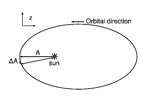
Figure 1: Laplace-Runge-Lenz vector, its variation and the orbital plane as the complex plane

Since the force due to the string gauge field is magnetic like CheungGRC0:2007 , we first check the precession caused by magnetic like force. After that we continue to analyze the effect of general power law central force.

2.1 Magnetic like force

For magnetic like force we have

$$\vec{\eta} = \frac{q}{m}\vec{v}\times\vec{B}$$ (3)

Assuming the magnetic field is pointing upward perpendicular to the solar plane in which all planets move counterclockwise, we have

$$\frac{d\vec{A}}{dt} = -\frac{q}{m}Bh\vec{v}-\frac{q}{m}(\vec{x}\cdot\vec{v})(\vec{v}\times\vec{B})$$ (4)

and for integral over time, denoted by $\Delta\vec{A}$,

$$\int d\vec{A}=-\frac{q}{m}\int Bh\vec{v}dt-\frac{q}{m}\int(\vec{x}\cdot\vec{v})(\vec{v}\times\vec{B})dt$$ (5)

Firstly let us check the first term. Because planet orbits all have very small eccentricities, we can assume a constant magnetic field over the whole orbit for each particular planet. Thus $B$ can be taken outside of the integral. The factor $h$ can also be taken outside because it depends only on the orbit and it is constant for the unperturbed orbit . Therefore the first term is proportional to

$$\int\vec{v}dt=\int d\vec{x}=\Delta\vec{x}$$ (6)

and vanishes for unperturbed orbit. Now we are left with only the second term. It can be simplified as follows

$$\int(\vec{x}\cdot\vec{v})(\vec{v}\times\vec{B})dt$$

$$= \int(\vec{v}\times\vec{B})d\left(\frac{1}{2}\vec{x}^{2}\right)=-\int\frac{1}{2}\vec{x}^{2}d(\vec{v}\times\vec{B})$$

$$= \vec{B}\times\int\frac{1}{2}\vec{x}^{2}\frac{d\vec{v}}{dt}dt=\vec{B}\times\left(-\frac{k}{2}\int\hat{x}dt\right)$$

$$= \vec{B}\times\left(-\frac{k}{2}\int\hat{x}\frac{1}{\omega}d\theta\right)=\vec{B}\times\left(-\frac{k}{2h}\int\hat{x}r^{2}d\theta\right)$$ (8)

where we have used partial integration and Newton’s second law $\vec{a}=-\frac{k\hat{x}}{|\vec{x}|^{2}}$ and $\omega$ is the angular velocity. Regarding the planetary motion plane as a complex plane, we can denote $\hat{x}$ by $\exp(i\theta)$, and for elliptic orbit with semimajor axis $a$ and eccentricity $e$, $r=\frac{a(1-e^{2})}{1-e\cos\theta}$, therefore

$$\int\hat{x}r^{2}d\theta=\left[a(1-e^{2})\right]^{2}\int\frac{\exp(i\theta)d\theta}{(1-e\cos\theta)^{2}}$$ (9)

Combining above formulas, we get

$$\Delta\vec{A} = i\frac{qkB}{2hm}\left[a(1-e^{2})\right]^{2}f(e)$$ (10)

where

$$f(e) = \int_{0}^{2\pi}\frac{\exp(i\theta)d\theta}{(1-e\cos\theta)^{2}}$$ (11)

Remembering that $\Delta\phi=\left|\frac{\Delta\vec{A}}{|\vec{A}|}\right|$, and Goldstein:mechanics ; Weinberg:gravitation

$$k = GM_{\odot}$$ (12)

$$L = hm=\sqrt{GM_{\odot}m^{2}a(1-e^{2})}$$ (13)

$$|\vec{A}| = eGM_{\odot}$$ (14)

we get

$$\Delta\phi=-\left(\frac{qB}{m}\right)\frac{1}{\sqrt{GM_{\odot}}}\left[a(1-e^{2})\right]^{\frac{3}{2}}\frac{f(e)}{2e}$$ (15)

$f(e)$ can be integrated exactly and is

$$f(e)=2\pi e(1-e^{2})^{-\frac{3}{2}}$$ (16)

and thus

$$\Delta\phi=-\left(\frac{qB}{m}\right)\frac{1}{\sqrt{GM_{\odot}}}\pi a^{\frac{3}{2}}$$ (17)

This is the angle precessed in one revolution, the precession rate in time is

$$\delta\dot{\omega}=-\left(\frac{qB}{m}\right)\frac{1}{\sqrt{GM_{\odot}}}\pi\left(\frac{a^{\frac{3}{2}}}{T}\right)$$ (18)

Note that the eccentricity disappeared here. Also note that one of Kepler’s law says that $\frac{a^{\frac{3}{2}}}{T}$ is a constant for planets in the solar system. But in later calculation we will not treat it as a constant but simply use the data of $a$ and $T$ to compute it.

2.2 Power law central force

For central force the time derivative of Laplace-Runge-Lenz vector simplies to

$$\frac{d\vec{A}}{dt}=\vec{\eta}\times\vec{h}$$ (19)

and thus

$$\Delta\vec{A} = \int\vec{\eta}\times\vec{h}dt=h\int\eta(r)\hat{x}\times\hat{z}dt$$ (20)

$$= \int\eta(r)r^{2}\left(\hat{x}\times\hat{z}\right)d\theta$$ (21)

where $\eta$ is the magnitude of the perturbation acceleration, outward from the center is defined to be positive. For general power law central force $\eta(r)=Kr^{n}$, using elliptic orbit equation $r=\frac{a(1-e^{2})}{1-e\cos\theta}$ and after some similar algebra as above, we get

$$\Delta\vec{A}=(-i)K\left[a(1-e^{2})\right]^{n+2}f_{n}(e)$$ (22)

where, as before, we used a complex number to represent the variation, and $f_{n}(e)$ is a function of eccentricity only, defined by

$$f_{n}(e)=\int^{2\pi}_{0}\frac{\cos\theta d\theta}{\left(1-e\cos\theta\right)^{n+2}}$$ (23)

This integral can be done exactly, the key equation is

$$\int^{2\pi}_{0}\frac{e^{i\theta}d\theta}{\left(1-\lambda\cos{\theta}\right)^{n}}$$ (24)

$$= \frac{2\pi}{(n-1)!}\left(-\frac{2}{\lambda}\right)^{n}\left(\frac{d}{dz}\right)^{n-1}\left(\frac{z}{z-z_{+}}\right)^{n}|_{z=z_{-}}$$

where $z_{\pm}=\frac{1}{\lambda}\pm\sqrt{\frac{1}{\lambda^{2}}-1}$. But an expasion in $e$ will be more illuminating. For planet orbits, we have $e\ll 1$, and we can expand the factor $\frac{1}{(1-e\cos\theta)^{n+2}}$ to

$$1-(n+2)(-e\cos\theta)+\mathcal{O}(e^{2})$$ (25)

Then to the first order of $e$,

$$f_{n}(e)\approx\int^{2\pi}_{0}(n+2)e\cos^{2}\theta d\theta=(n+2)e\pi$$ (26)

and for the Laplace-Runge-Lenz vector variation we have

$$\Delta\vec{A}\approx(-i)K\left[a(1-e^{2})\right]^{n+2}(n+2)e\pi$$ (27)

Recalling $|\vec{A}|=eGM_{\odot}$, the angle precessed in one revolution $\Delta\phi=|\frac{\Delta\vec{A}}{\vec{A}}|$ is

$$\Delta\phi\approx\frac{K\pi}{GM_{\odot}}\left[a(1-e^{2})\right]^{n+2}(n+2)$$ (28)

This precession angle formula is for the most general power law central force perturbations. Following are some example applications.

Schwarzschild space-time

For Schwarzschild space-time a test particle’s orbit obeysMisner:gravitation

$$\tilde{E}^{2}-\left(1-2\frac{M}{r}\right)\left(1+\frac{\tilde{L}^{2}}{r^{2}}\right)=\dot{r}^{2}$$ (29)

where $\tilde{E}$ and $\tilde{L}$ are the energy and the angular momentum per unit mass, respectively. After expanding it is

$$\left(\tilde{E}^{2}-1\right)+\frac{2M}{r}-\frac{\tilde{L}^{2}}{r^{2}}+\frac{2M\tilde{L}^{2}}{r^{3}}=\dot{r}^{2}$$ (30)

On the other hand, in classical mechanics we have

$$\frac{1}{2}m\dot{r}^{2}+V+\frac{L^{2}}{2mr^{2}}=E$$ (31)

or

$$\frac{2E}{m}-\frac{2V}{m}-\frac{L^{2}}{m^{2}r^{2}}=\dot{r}^{2}$$ (32)

Comparing this to eq.(30), it can be read out that in the Newtonian limit, we should have

$$\tilde{E}^{2}-1 = \frac{2E}{m},$$ (33)

$$\frac{\tilde{L}^{2}}{r^{2}} = \frac{L^{2}}{m^{2}r^{2}}$$ (34)

$$\frac{2M}{r}+\frac{2M\tilde{L}^{2}}{r^{3}} = -\frac{2V}{m}$$ (35)

from the last of the three equations we know, with some dimensional conversion, the total gravitational potential in the Newtonian limit is

$$\Phi=-\frac{GM}{r}-\left(\frac{GM}{c}\right)^{2}a(1-e^{2})\frac{1}{r^{3}}$$ (36)

The first term is the usual Newtonian potential. The second term considered as the perturbation potential causing precession gives acceleration

$$\eta=-\left(\frac{GM}{c}\right)^{2}a(1-e^{2})\frac{3}{r^{4}}$$ (37)

thus $K=-3\left(\frac{GM}{c}\right)^{2}a(1-e^{2})$ and $n=-4$. By (28) the corresponding precession per revolution is

$$\Delta\phi=\frac{6\pi GM_{\odot}}{c^{2}}\frac{1}{a(1-e^{2})}$$ (38)

This is precisely the one directly derived from general relativityMisner:gravitation , e.g it is the $43^{\prime\prime}/cy$ for the planet Mercury.

Solar system with dark matter

Equation (28) can also be used to derive precession caused by possible dark matter spherically distributed in the solar system. In this case we have

$$\eta(r)=-\frac{4\pi}{3}\rho_{0}Gr$$ (39)

where $\rho_{0}$ is the dark matter density, and the corresponding precession is

$$\Delta\phi=-\frac{4\pi^{2}\rho_{0}}{M_{\odot}}\left[a(1-e^{2})\right]^{3}$$ (40)

After some dimensional conversion, this result is the same with the one in Gron:1995 except that the factor $(1-e^{2})$ is absent there. It is because Gron:1995 considered only circular orbit. The result here works also for ellipse.

Generally the equation (28) provides a convenient way to judge whether a power law perturbation causes prograde or retrograde precession. $n=-2$ is a critical value. The result is summarized in table 1.

	$n<-2$	$n=-2$	$n>-2$
$K<0$	$+$	$0$	$-$
$K>0$	$-$	$0$	$+$

Table 1: Sign of $\Delta\phi$ for perturbations of form $\eta(r)=Kr^{n}$. “$+$” for prograde, “$-$” for retrograde.

3 String field strength from precession in solar system

Here we will use the anomalous precession data to calculate the string field strength in the solar system. We attribute all the anomalous precession Iorio:2009 to the magnetic like force due to the string field. We are interested in the quantityCheungGRC0:2007

$$\Omega=\frac{QH}{m}$$ (41)

where $\frac{Q}{m}$ and $H$ are the string charge-to-mass ratio and field strength, respectively. $\Omega$ is the string field strength in dimension $s^{-1}$. The corresponding one in electromagnetism is $\frac{eB}{m}$. In this dimension, we can compared it with strengthes of other magnetic-like forces. We just need to convert the strength into the dimension $s^{-1}$, e.g $\frac{eB}{m}$ for electromagnetism. To calculate the strength from precessions we invert (18) and get

$$\Omega=(-\delta\dot{\omega})\sqrt{GM_{\odot}}\frac{T}{\pi a^{\frac{3}{2}}}$$ (42)

Because relative errors from other parts are all tiny compared to the one of the precession rate, the error of $\Omega$ can be computed by

$$Err(\Omega)=Err(\delta\dot{\omega})\sqrt{GM_{\odot}}\frac{T}{\pi a^{\frac{3}{2}}}$$ (43)

or simply

$$\left|\frac{Err(\Omega)}{\Omega}\right|=\left|\frac{Err(\delta\dot{\omega})}{\delta\dot{\omega}}\right|$$ (44)

The value of $\Omega$ calculated are shown in table 2. And the diagram is shown in Fig.2. Orbital datas are from HORIZON . Precession datas are from Iorio:2009 .

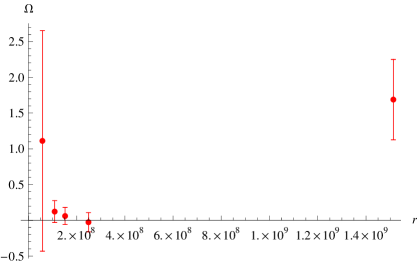
Figure 2: $\Omega(1\times 10^{-17}s^{-1})$ versus distance $r(km)$ to the Sun

The center values of $\Omega$ for the inner planets exhibit a decreasing pattern with respect to $r$, although long error bars allow also the case of vanishing string field. At the Saturn, $\Omega$ is nonzero within one $\sigma$. However, as mentioned in Iorio:2009 , the error bar at the Saturn may actually be bigger, in which case the value of precession or $\Omega$ then vanish. More precise experiments on precessions are needed to get more definite conclusions regarding $\Omega$ (or anomalous precessions) in the solar system. Inspired by this decreasing pattern, in the next section we will try to fit data of inner planets with a (nearly) power law profile.

No matter how critically we take the calculated result of $\Omega$ here, it is certainly true that the upper limit of $\Omega$ at the solar system is on the order of $10^{-17}s^{-1}$. As a compare, let us note that for the real magnetic field near earth, since $\frac{e}{m}=1.76\times 10^{11}C/kg$ and the interplanetary magnetic field there is on the order of $10^{-9}T$, we have $\Omega_{em}\sim 100s^{-1}$. In that sense, the string field strength is $10^{19}$ times smaller than the real magnetic field. Then arises the question that why we not use the real magnetic field directly to explain the precession, now that we find the required field strength is so much smaller than observed real magnetic field. One reason is that matter is electrically neutral, but assumed in our model to be stringly charged. The real magnetic field can act on neutral matter only through dipole dipole interaction, which, as explained in the appendix, for several reasons does not contribute to planet precession. Another question about this string model is, now we are assuming matter is stringly charged and being acted on by the corresponding magnetic field for this charge, then is there or where is an electrical interaction between stirngly charged matter. After all, so far we seem to be assuming all matter take the “same” (if there are more than one kind of charge) kind of charge. This question lies outside of our current model and need more theoretical investigations into this string charge. As for the model used here, we can say that we are using an electromagnetic-like model with magnetic field interactions only.

It is interesting to calculate the extra acceleration due to the string field for objects on the earth. Since the field strength is got for the rest frame relative to the Sun, the velocity of objects on the earth should be almost the same with the velocity of the earth relative to the Sun, i.e $30km/s$. The corresponding acceleration produced is $\sim 10^{-13}m\cdot s^{-2}$.

Name	Mercury	Venus	Earth	Mars	Saturn
$\delta\dot{\omega}(10^{-4}~{}^{\prime\prime}/cy)$	$-36\pm 50$	$-4\pm 5$	$-2\pm 4$	$1\pm 5$	$-60\pm 20$
T(y)	0.240846	0.6151970	1.0000175	1.8808	29.4571
a(km)	57909100	108942109	152097071	249209300	1513325783
e	0.205630	0.0068	0.016710219	0.093315	0.055723219
$\Omega(10^{-17}s^{-1})$	$1.11$	$1.22\times 10^{-1}$	$5.99\times 10^{-2}$	$-2.69\times 10^{-2}$	$1.68794$

Table 2: Planets data and values of $\Omega$

More on the Saturn. One thing special about the Saturn is that it belongs to gas giant while all other planets considered here are small and solid planets of the inner planet family of the solar system. As in electromagnetic theory, the content and structures of planets may affect their interactions with the string field, which might explains the anomalous behavior of the Saturn. This argument can be supported if anomalous precession behaviors similar to the Saturn’s can be observed on other outer planets.

4 Profile fitting of precession in solar system

The decreasing pattern of $\Omega$ for inner planets with respect to $r$ indicates it might be useful to fit these values with a power law term. Presumably we could attribute this $r$ dependent term to the Sun from which $r$ is measured. On the other hand, note that $\Omega$ at the Mars is negative, although it seems also sitting on the same curve passing the first three inner planets. One possible configuration for $\Omega$ then is that, in addition to the power law term, there is also a weak constant background $\Omega$ with opposite direction to the $\Omega$ from the Sun. The background might be provided by all other matter in the universe. The Milky Way should be the most important source of influence. Thus here we try to fit field strength at different inner planets with the following profile,

$$\Omega(r)=A+Br^{-a}$$ (45)

For the actual fitting on computer, the profile used is

$$\Omega(r)=\Omega_{0}+\Omega_{1}\left(\frac{r}{10^{7}km}\right)^{-a}$$ (46)

The best fitting parameters for this profile is

$$\Omega_{0} = -0.0223787\times 10^{-17}s^{-1}$$ (47)

$$\Omega_{1} = 260.504\times 10^{-17}s^{-1}$$

$$a = 3.09953$$

It is interesting to know the relative strength of the two components from the Sun and the constant background, the result is shown in table 3.

Planet	Mercury	Venus	Earth	Mars
ratio	50.3	7.1	2.5	0.54

Table 3: relative strength: power law term/constant term

The power law term decreases with $r$ quickly relative to the background. We can say that in most areas in the solar system, the string field would just be around that background, which is on the order of $10^{-19}$Hz.

Note that $a$ is found to be near 3, which is exactly the power for a dipole field. It means that the string field interaction between the sun and planets is similar to that between a magnetic dipole and charged particles.

Note that the fitting tells us the constant background in the solar system is negative. This is good news for the string model. As in electromagnetism, we expect the string gauge field in a galaxy be generated by the rotation of (stringly charged) matter in the galaxy, just like rotating electric charge would generate magnetic field. Because the Sun and planets in the solar system rotate in opposite direction of that of stars’ rotation in the Milky Way, therefore naively we would expect the background field to be negative if we consider the one from the Sun as positive. And this is exactly what the profile fitting told us. Only data in the solar system was used, but the conclusion is for the whole Milky Way, specifically for its rotation direction. However, this conclusion is not so robust as it might seem. Firstly, the long error bars of precession weaken the conclusion from profile fitting. Secondly, since the Sun contains 99% of the total mass in the solar system, all planets are well outside of the major mass concentration of the solar system, but we do not have enough experimental data to say whether or not the solar system lies in the major mass concetration of the Milky Way. As in ordinary electromagnetic theory, for a right handed current disk the magnetic field is downward outside of the major current distribution, but upward if we go into the current disk somewhere, specifically at the center of the disk. There is a place within the concentration where the magnetic field changes its sign. Thus even if the Milky Way is rotating in opposite direction from the solar system, if the Sun is too close inside the major mass concentration of the Milky Way, the background therefrom should still be positive. If we believe the negative background from the profile fitting, then it necessarily implies that the solar system does not sit very close to the center of the Milky Way. This is reasonalble assumption but can not be verified for lack of precise data for mass distribution in the Milky Way.

5 $\Omega$ from rotation curve of the Milky way

Above from anomalous precession we have obtained $\Omega$ in the solar system. The background value there in large part should come from other matter in the Milky Way altogether. On the other hand, by the same idea used in CheungGRC1:2008 , we can also estimate $\Omega$ at the solar system by the rotation curve of the Milky Way. A natural check of the string field model would be to compare $\Omega$ from precessions in the solar system with $\Omega$ from rotation curve of the Milky Way.

As mentioned above, we do not have sufficient data to know if the solar system is far away enough from the Milky Way center such that its velocity is increased by the string field. If we trust the negative background got from precession fitting, the velocity of the solar system in the Milky Way is increased by the string field. (It means the sun is in the lifted part of the rotation curve.) In the rest part of this section we will assume the velocity of the solar system is increased by the string field.

Using the idea in CheungGRC1:2008 , we can make a rough estimate of $\Omega$ in the Milky way as follows. In the string model, the total force on the sun is composed of only the gravitational attraction from visible mass in the Milky Way and the magnetic-like force from the string field. The gravitational force decreases quickly, and the magnetic like force always increases, with increasing $r$. Now observe that at the position of the sun the rotation curve is already fairly flat Sofue:1997 ; Sofue:1999 ; Florido:2000 . Therefore on the sun the gravitational force should be comparable or even neglectable with respect to the magnetic-like force from the field. ThenCheungGRC0:2007

$$m\frac{v^{2}}{r}\approx QHv$$ (48)

and thus

$$\Omega\approx\frac{v}{r}$$ (49)

For the sun Sofue:1997 ; Sofue:1999 ; Florido:2000 , $v_{\odot}\approx 200km\cdot s^{-1}$ and $r_{\odot}\approx 7.6kpc$. So

$$\Omega_{\odot}\approx 26s^{-1}\cdot\frac{km}{kpc}=8.5\times 10^{-16}s^{-1}$$ (50)

This is the upper limit on $\Omega$ at the Sun. Since there is still a portion of distance further out to nearly $20kpc$ where the curve is quite flat (with velocity $\sim 200km\cdot s^{-1}$) Sofue:1997 ; Sofue:1999 ; Florido:2000 , we could have used these distances instead of $7.6kpc$. In that case, it is still safe to say the upper limit of $\Omega$ is on the order $10^{-16}s^{-1}$. This is the strength of the field component perpendicular to the galactic plane. To convert it to the solar system, notice that the north galactic pole and the north ecliptic pole form an angle of 60.2^∘ (which means the field in the solar system would be reduced almost by half ), and the milky way rotates clockwise when viewed from north galactic pole (which means the field is negative in the solar system). Therefore from the rotation curve of the milky way the upper limit of the effective field strength in the solar system due to matter in the milky way is $-10^{-17}\sim-10^{-16}s^{-1}$. This magnitude is close to the one found by direct precession calculation without the profile assumption, but it is not the case for field direction. The precession indicates the field in the solar system is positive, while rotation curve of the milky way implies it is negative. One possible explanation is that at places near the Sun the field is dominated the positive field generated by the Sun. And on the other hand, the profile fitting of precession, apart from a dipole like part due to the Sun, indeed gives a negative background ($-0.02\times 10^{-17}s^{-1}$). However the magnitude there is smaller by almost two orders of magnitude.

6 $\Omega$ from rotation curves fitting of 22 galaxies

In CheungGRC1:2008 rotation curves of 22 galaxies were fitted with the string model and $\Omega$ is found to lie in the range $0.1\sim 16$. There the dimension for $\Omega$ is $s^{-1}\frac{km}{kpc}$. Thus $\Omega=1$ from fitting means $\Omega=3\times 10^{-17}s^{-1}$. Considering the additional factor of $\frac{1}{2}$ in the definition of the $\Omega$ in CheungGRC1:2008 , it means $\Omega$ using the definition of the current paper is in the range $6\times 10^{-18}\sim 1\times 10^{-15}s^{-1}$ for these 22 galaxies. This range of magnitude covers the value in the Milky Way got from rotation curve, and also part of those got from precesseion in the solar system.

According to the string model, considering its analogy with electromagnetism, it is reasonable to expect the average field strength to be proprotional to $M^{\alpha}R^{-\beta}$ where $M$ is the total luminous matter in the galaxy and $R$ is the size scale of the galaxy. With the assumption that $L\propto M$ where $L$ represents the luminosity of the galaxy, it is thus interesting to see if there is any such relation between $\Omega$, $R$ and $L$ in the fitting result for the 22 galaxies. This serves as a consistency check for the string model. To be more specific we will first use the electromagnetism analogy to get such a relation theoretically as follows, and then check it with experimental data for these 22 galaxies. Consider a group of electrons azimuthal symmetrically distributed and in rotation around the $z$ axis. Let us look at the magnetic field at the center of this distribution , the determining physical quantities are: the magnetic constant $\mu_{0}$, mass density scale $\rho_{0}$, distribution size scale $R_{0}$ and rotational angular velocity scale $\omega_{0}$. (Other determining factors include the shape and the spatial dependence of the mass distribution, the spacial distribution of the angular velocity. These factors do not change the result of dimensional analysis but change the proportional constant.) By dimensional analysis, we have

$$B\propto\mu_{0}\cdot\rho_{0}\cdot\omega_{0}\cdot R_{0}^{2}$$ (51)

Using the total charge $Q\propto\rho_{0}\cdot R_{0}^{3}$, and defining $v_{0}=\omega_{0}\cdot R_{0}$, we have

$$B\propto\mu_{0}\cdot Q\cdot R_{0}^{-2}\cdot v_{0}$$ (52)

Note that $v_{0}$ is the rotational velocity scale for the galaxy. Translating to the language of the string model, it is

$$\Omega\propto Q\cdot R_{0}^{-2}\cdot v_{0}$$ (53)

The proportional constant here depends only on the mass and angular velocity distributions, or abstractly on the galaxy type. Thus galaxies with similar mass distribution profile and rotation curve shapes should have similar constants of proportionality. Now recall $M\propto Q$, where the proportional constant is universal and thus the same for all galaxies. Furthermore we also use the assumption $L\propto M$. Thus

$$\Omega\propto L\cdot R_{0}^{-2}\cdot v_{0}$$ (54)

To relate $v_{0}$ to $L$ we use the Tully-Fisher relation which says $L\propto\Delta V^{\alpha}$ where $\alpha$ is around $2.5\pm 0.3$ and $\Delta V$ is the velocity width of the galaxyTully&Fisher:1977 . The proportional constant in the Tully-Fisher relation is galaxy type independent. Since $v_{0}$ is the overall scale for $\Delta V$, we have also $L\propto(v_{0})^{\alpha}$. Using this in (54), we get

$$\Omega\cdot R_{0}^{2}\propto L^{1+\frac{1}{\alpha}}$$ (55)

which after taking logrithms

$$\ln\left(\Omega R_{0}^{2}\right)=\left(1+\frac{1}{\alpha}\right)\ln\left(L\right)+\ln\kappa$$ (56)

where $\kappa$ is the proportional constant in the relation (55). The log-log diagram is shown in Fig.3.

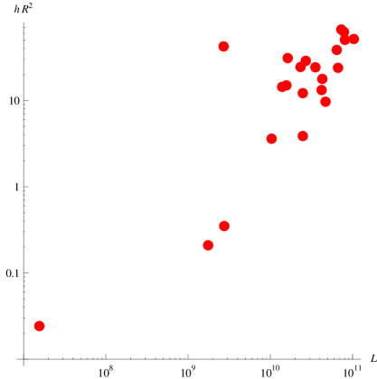
Figure 3: luminosity to $\Omega R^{2}$ log-log plot

There is indeed a trend of a linear relation in the “main” part of the diagram. The slope of the line is about $\frac{3}{2}$, quite close to the $1+\frac{1}{2.5\pm 0.3}$ derived theoretically. 2 points seems to lie outside of the “main” part, i.e one at the lower left corner for the dwarf galaxy m81dwb, another one for NGC4236 at the left of the upper right group. One possible explanation for these 2 galaxies might be that galaxy types of these two are too different from the rest and thus their $\ln\kappa$ deviated more from those in the “main” part. Actually in terms of morphology type, NGC4236 is SBdm, which is the most irregular one among the regular types, while m81dwb is the only irregular one among the 22 galaxies NED , all others are more or less regular galaxies. Presumably these two lie on another line for irregular galaxies which is parallel to the line passing the rest. Furthermore there might be series of parallel lines for different types of galaxies. However, statistical error from the small size of this data set makes above arguments weak. On the other hand, it does not kill the model either. Analysis of this kind for a larger number and more types of galaxies could make the situation clearer.

7 Summary

We analyzed the precession motion under influences of magnetic like force and power law central force. The result for magnetic like force is later used in computing $\Omega$ in the solar system. The result for power law central force is tested in two examples, i.e Schwarzschild space-time and solar system with dark matter, and found to be in agreement with analysis by other methods. For power law central force, a simple criterian judging pro- or retrograde precession is derived, $n=-2$ turns out to be a critical value between pro- and retrograde cases.

Based on the theoretical analysis of precesssion, assuming all remaining anomalous precessions are caused by the string field, we calculated the string field strength in the solar system. It is found to be on the order of $10^{-17}s^{-1}$. Except the data of the Saturn, anomalous precessions of other planets considered in this paper indicate a string field of almost $\frac{1}{r^{3}}$ decreasing pattern, where $r$ is the distance to the Sun.

For the string field strength in the solar system, a profile fitting is further done to compare with the result directly calcualted from precession. We assumed the string field consists of two parts. One from the Sun, which goes as $\frac{1}{r^{a}}$. The second part comes from the rest of the Milky Way, which is a constant background within the solar system region. The part due to the Sun is found to be nearly a dipole field, i.e $\frac{1}{r^{3}}$. The background is found to be negative, which, when combined with analysis using electromagnetism analogy, correctly matches with the fact that the solar system and the Milky Way rotate in opposite directions.

As an independent check of the calculated result of the string field in the solar system, we used the rotation curve of the Milky Way to estimate the string field strength in the Milky Way, which contains the solar system. The estimation gives a similar order of magnitude with that got from precessions. But the direction is opposite. If we consider the result from profile fitting, then the background direction agrees with the one predicted by Milky Way rotation curve, but the magnitude is smaller by 2 orders of magnitude.

For 22 galaxies fitted in CheungGRC1:2008 , the string field strength is found to span a range just around that of the solar system, or the Milky Way. Note that here the strength is found by precise fitting of rotation curves of the 22 galaxies, which is a completely independent method from fitting precession.

Based on an analysis of an electromagentism analogy, we derived a relation between $\Omega R^{2}$ and luminosity. This relation is then checked by fitting result from CheungGRC1:2008 . Except for two galaxies, the data for the other 20 galaxies all satisfy the derived relation to a good degree. This way the string model survived one model consistency check.

In summary of analysis about the string field strength $\Omega$, we used three kinds of observations to find corresponding values of $\Omega$: 1) rotation curves of 22 galaxies, 2) rotation curve of the Milkyway and 3) anomalous precessions in the solar system(, which is also in the Milkyway). All the situations are summarized in Table.4, and we can see there is no obvious inconsistency in using the string model for various objects and obsevations.

	Solar System $\subset$	Milky Way	22 other galaxies
Rotation Curve		$|\Omega|\lesssim 10^{-16}$	$6\times 10^{-18}\lesssim|\Omega|\lesssim 10^{-15}$
Precession	$|\Omega|\lesssim 10^{-17}$

Table 4: Summary (Dimension for $\Omega$ is $s^{-1}$). The first column indicates the kind of observation used.

Appendix A: Solar system magnetic field and its effect on planet perihelion precession

References for this appendix are Parker ; Parker:1958 ; Encyclopedia:1997 ; Meyer:Parker:Simpson:1956 ; Babcock:1961 . The Sun and most planets in the solar system have magnetic field due to dynamo effect. If we treat both the Sun and the planet as magnetic dipoles interacting in vaccum (which leads to a central force with $n=-4$), using data of magnetic fields of the Sun (around $1\sim 2$ gauss at the polar region) and the Earth (around 0.6 gauss at the polar region), we can find the corresponding precession produced is nearly $10^{-6}$arcsec/cy, which is 2 orders of magnitude smaller than the observed one. In fact the magnetic field in the solar system is much more complicated than those produced by several dipoles in vacuum. First the solar system is not empty but filled with particles emitted from the Sun, i.e the solar wind. Charged particles lock with it the magnetic field of the Sun and spread it all around in the solar system. From the Sun to about the position of the Earth, the magnetic force line is parrell to the radial stream of solar wind particle and falls off by $r^{-2}$. From the position of the Earth to about position of the Mars is a field free region with $B<10^{-6}$ gauss. Further out to the position of the Jupiter is a region with disordered magnetic field with $B\sim 10^{-5}$ gauss. For precession, the most important feature of the solar system field is that it is oscillating. Firstly, for the Sun the magnetic dipole axis is inclined relative to the rotational axis. This leads to an oscillating neutral current sheet. Therefore planets on the ecliptic plane is above the netral current sheet for half of solar self rotation period, below for another half. Since field directions above and below the netral current sheet is opposite, the magnetic force experienced by the planets also change directions within one self rotation of the Sun. Secondly, the magnetic field of the Sun also changes direction every 22 years due to its differential rotation, which leads to another oscillation of magnetic field on the planets. Alltogether these two oscillations render the magnetic field effect on precession neglectable with respect to other accumulating effects.

References

- (1) Y.K.E. Cheung, K. Savvidy, H.C. Kao (2007), astro-ph/0702290
- (2) Y.K.E. Cheung, F. Xu (2008), 0810.2382
- (3) L. Iorio, The Astronomical Journal 137 3615 (2009)
- (4) H. Goldstein, C.P. Poole, J.L. Safko, Classical Mechanics, 3rd Edition (Addison Wesley, 2002)
- (5) S. Weinberg, Gravitation and cosmology: principles and applications of the general theory of relativity (Wiley, 1972)
- (6) C. Misner, K. Thorne, J. Wheeler, Gravitation (W. H. Freeman, 1973)
- (7) Ø. Grøn, H.H. Soleng (1995), astro-ph/9507051
- (8) Horizon web interface, http://ssd.jpl.nasa.gov/?horizons
- (9) M. Honma, Y. Sofue, Publ. Astron. Soc. Japan 49 (1997)
- (10) Y. Sofue, Y. Tutui, M. Honma, A. Tomita, T. Takamiya, J. Koda, Y. Takeda (1999), astro-ph/9905056
- (11) E. Battaner, E. Florido, Fund. Cosmo Phys. 21 (2000), astro-ph/0010475
- (12) R.B. Tully, J.R. Fisher, J. R. Astronomy and Astrophysics, vol. 54, no. 3 pp. 661–673 (1977)
- (13) M. Roberts, Astronomical Journal 74 (1969)
- (14) Nasa/ipac extragalactic database, http://nedwww.ipac.caltech.edu
- (15) E.N. Parker, Astrophysical Journal 128 (1958)
- (16) E.N.Parker, Physical Review 110 (1958)
- (17) J.H. Shirley, R.W. Fairbridge, Encyclopedia of Planetary Sciences (1997)
- (18) P. Meyer, E.N. Parker, J.A. Simpson, Physical Review 104 (1956)
- (19) H.W. Babcock, Astrophysical Journal 133 (1961)