Experimental confirmation of chaotic phase synchronization in coupled time-delayed electronic circuits

Abstract

We report the first experimental demonstration of chaotic phase synchronization (CPS) in unidirectionally coupled time-delay systems using electronic circuits. We have also implemented experimentally an efficient methodology for characterizing CPS, namely the localized sets. Snapshots of the evolution of coupled systems and the sets as observed from the oscilloscope confirming CPS are shown experimentally. Numerical results from different approaches, namely phase differences, localized sets, changes in the largest Lyapunov exponents and the correlation of probability of recurrence ($C_{CPR}$), corroborate the experimental observations.

Chaotic phase synchronization (CPS) refers to the coincidence of characteristic time scales of interacting chaotic dynamical systems, while their amplitudes remain chaotic and often uncorrelated Pikovsky et al. (2001); Boccaletti et al. (2002). CPS plays a crucial role in understanding a large class of weakly interacting nonlinear dynamical systems and has been demonstrated both theoretically and experimentally in a wide variety of natural systems Scannel et al. (1999); Varela et al. (1998, 1999); Grenfell et al. (2001); RosaJr. et al. (2003); Volodehenko et al. (2001); Maza et al. (2000); Tass et al. (1998); Maraun and Kurths (2005); Vicent et al. (1998). Despite our substantial understanding of the phenomenon of CPS and its potential applications in low-dimensional systems, only a very few studies on it have been reported in time-delayed systems, which are essentially infinite-dimensional in nature Senthil2 et al. (2006); Suresh et al. (2010). Due to the highly non-phase-coherent chaotic/hyperchaotic attractors with complex topological properties exhibited by these systems in general, it is often impossible to estimate the phase explicitly and to identify CPS.

Recently, we have introduced a nonlinear transformation to recast the original non-phase-coherent attractors into smeared limit-cycle attractors to enable to estimate the phase explicitly and to identify CPS in time-delay model systems for the first time in the literature Senthil2 et al. (2006). In this paper, we report the first experimental demonstration of CPS in coupled time-delay systems using electronic circuits. We have also experimentally implemented the methodology of localized sets Pereira et al. (2007) and show that this is a crucial and a general framework for characterizing CPS even in non-phase-coherent attractors of time-delay systems Senthil2 et al. (2006); Suresh et al. (2010). Our results will open up the possibility of experimental realization of CPS in other physical systems with delay and to their potential applications.

Figure 1: Schematic diagram of the unidirectionally coupled time-delay analog circuits with threshold nonlinearity. ND1 and ND2 are nonlinear device units; delay unit consists of $10$ pairs of capacitors of $470nF$ and inductors of $12mH$. $R_{1}=R_{2}=1.86k\Omega$; $C_{1}=C_{2}=100nF$ and $A$ is the op-amp difference amplifier.

In particular, we will demonstrate the existence of CPS in unidirectionally coupled time-delay electronic circuits with threshold nonlinearity in both chaotic and hyperchaotic regimes experimentally (Note that bidirectional coupling can also work equally well). In addition to the snapshots of time series of both systems as seen from the oscilloscope, we have used the framework of localized sets Pereira et al. (2007) to characterize the existence of CPS in the above systems both experimentally and numerically. To investigate localized sets, we have considered the ‘event’ as maxima of the flow of the drive system and recorded the response system to obtain the ‘sets’, whenever a maximum occurs in the drive system and vice versa. The sets are then superimposed on the drive (response) attractor, which get localized on it during CPS but spread over the entire attractor when the systems evolve independently. Further, we have also confirmed the existence of CPS numerically using the localized sets, the largest Lyapunov exponents of the coupled time-delay systems and also with another independent approach based on recurrence analysis, namely the correlation of probability of recurrence ($C_{CPR}$) Marwan et al. (2007).

Figure 2: Nonlinear device unit (ND) of Fig.1: Actual circuit implementation of the nonlinear activation function consisting of diodes $D_{1}=D_{2}=1N4148$, resistor $R_{1}=R_{7}=1k\Omega,R_{2}=R_{3}=10k\Omega,R_{4}=2k\Omega,R_{5}=3k\Omega,R_{6}=10.4k\Omega$ and $R_{8}=5k\Omega$ and threshold control voltages $V_{1}=V_{2}=0.7V$ along with different amplifying stages ($OA_{1}=OA_{2}=OA_{3}=uA741$).

Figure 3: (color online) Snapshots of the time evolution of both coupled systems indicating the existence of CPS in (a) chaotic regime and (b) hyperchaotic regime. $x$-axis: time ($1$ unit= $1.0ms$), $y$-axis: voltage ($1$ unit= $1.0V$).

The coupled electronic circuit investigated here is shown in Fig. 1 as a block diagram. The individual time-delay units have a ring structure and comprise of a diode based nonlinear device unit (ND) (Fig. 2), a variable time-delay unit (DELAY) along with an integrator ($R_{0}C_{0}$) unit.

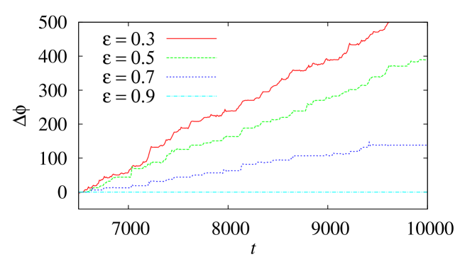
Figure 4: (color online) Phase difference for different values of $\varepsilon=0.3,0.5,0.7$ and $0.9$ and $\tau=1.33$.

The dynamics of the individual circuit in Fig. 1 is represented by the delay differential equation $R_{0}C_{0}\frac{dU(t)}{dt}=-U(t)+F[k_{f}U(t-T_{d})]$, where $U(t)$ is the voltage across the capacitor $C_{0}$, $U(t-T_{d})$ is the voltage across the delay unit (DELAY), $T_{d}=n\sqrt{LC}$ is the delay time, $n$ is the number of $LC$ units and $F[k_{f}U(t-T_{d})]$ is the static characteristic of the ND shown in Fig. 2. The block diagram (Fig. 1) also contains a differential amplifier circuit (A) with a gain $\varepsilon=R_{f}/R$ used to find the difference between the two voltage signals $U_{1}$ and $U_{2}$. By changing the feedback resistance $(R_{f})$, the coupling strength $\varepsilon$ can be varied.

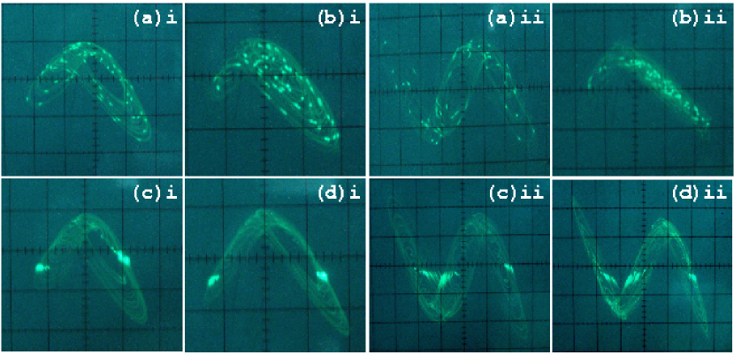
Figure 5: (color online) Experimental characterization of CPS using the framework of localized sets in the chaotic regime (i) for $\tau=1.33$ and in the hyperchaotic regime (ii) for $\tau=6.0$. Sets in the drive and the response systems are distributed in (a) and (b) for $\varepsilon=0.3$ indicating the asynchronous state and localized in (c) and (d) for $\varepsilon=0.9$ indicating CPS, respectively. $x$-axis : voltage $U(t)$ ($1$ unit= $0.5V$), $y$-axis: voltage $U(t-T_{d})$ ($1$ unit= $2.0V$).

The normalized evolution equation corresponding to the coupled time-delay electronic circuits (Fig. 1) is represented as Srinivasan et al. (2007, 2007)

$$\dot{x}= \,-x(t)+b_{1}f\left[x(t-\tau)\right],$$

$$\dot{y}= \,-y(t)+b_{2}f\left[y(t-\tau)\right]+\varepsilon(x(t)-y(t)),$$ (1)

where $x(t)=y(t)=\frac{U(t)}{U_{s}}$, $\hat{t}=\frac{t}{R_{0}C_{0}}$, $\tau=\frac{T_{d}}{R_{0}C_{0}}$, and $b=k_{f}=1+(\frac{R_{8}}{R_{7}})$ are dimensionless circuit variables and parameters. The function $f(x(t-\tau))=F(U(t-T_{d}))$ is taken to be a symmetric piecewise linear function defined by Srinivasan et al. (2007, 2007)

$$f(x)=Af^{*}-Bx.$$ (2a)

Here

$$f^{*}=\left\{\begin{array}[]{cc}-x^{*}&\;\;\;\;\;\;x<-x^{*},\\ x&\;\;\;\;\;-x^{*}\leq x\leq x^{*},\\ x^{*}&\;\;\;\;\;\;x>x^{*},\end{array}\right.$$ (2e)

where $x^{*}$ is a controllable threshold value and can be altered by adjusting the values of voltages $V_{1}$ and $V_{2}$. $A=(R_{6}/R_{4})$ and $B=(R_{6}/R_{5})$ are positive parameters. The estimated normalized values turn out to be $x^{*}=0.7$, $A=5.2$, $B=3.5$, $b_{1}=1.2$ and $b_{2}=1.1$ in accordance with the values of the circuit elements. The parameter mismatch $b_{1}\neq b_{2}$ contributes to the non-identical nature of the coupled time-delay systems. In the following, we will demonstrate the existence of CPS as a function of the coupling strength $\varepsilon$ in both chaotic and hyperchaotic regimes for suitable values of the delay time $\tau$.

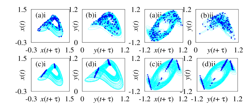
Figure 6: (color online) Numerical confirmation of CPS using the framework of localized sets in the chaotic regime (i) for $\tau=1.33$ and in the hyperchaotic regime (ii) for $\tau=6.0$. Sets in the drive and the response systems are distributed in (a) and (b) for $\varepsilon=0.3$ indicating the asynchronous state and localized in (c) and (d) for $\varepsilon=0.9$ indicating CPS, respectively.

The snapshots of the time series of both drive and response systems as seen from the oscilloscope are shown in Fig. 3(a) in the chaotic regime for the delay time $\tau=1.33$ and the coupling strength $\varepsilon=0.9$, indicating the evolution of both systems in-phase with each other. Similarly, the snapshots of the time series evolving in-phase with each other in the hyperchaotic regime for the delay time $\tau=6.0$ are shown in Fig. 3(b) for $\varepsilon=0.7$. The phase differences calculated numerically from the evolution equations, Eq. (Experimental confirmation of chaotic phase synchronization in coupled time-delayed electronic circuits), using the Poincaré section technique Pikovsky et al. (2001); Boccaletti et al. (2002) for different values of $\varepsilon$ are illustrated in Fig. 4, indicating the existence of CPS for $\varepsilon=0.9$ with $\tau=1.33$. The existence of CPS is further characterized both experimentally and numerically by using the framework of localized sets Pereira et al. (2007).

Figure 7: Confirmation of CPS in the chaotic regime using (a) Four largest Lyapunov exponents and (b) Correlation of probability of recurrence ($C_{CPR}$).

The sets obtained by sampling the time series of one of the systems whenever a maximum occurs in the other one are plotted along with the chaotic attractor of the same system for the delay time $\tau=1.33$ both experimentally and numerically in Figs. 5 and 6, respectively. The sets distributed over the entire attractor of both the drive [Figs. 5(a)i and 6(a)i] and the response [Figs. 5(b)i and 6(b)i] systems for the coupling strength $\varepsilon=0.3$ indicate that the time-delay systems evolve independently. The sets that are localized on the chaotic attractor of both the drive [Figs. 5(c)i and 6(c)i] and the response [Figs. 5(d)i and 6(d)i] systems for the coupling strength $\varepsilon=0.9$ correspond to a perfect locking of the phases of both systems as confirmed by the zero phase difference plotted in Fig. 4.

Next, we confirm the synchronization transition using the largest Lyapunov exponents of the coupled time-delay systems and the $C_{CPR}$ Marwan et al. (2007). The four largest Lyapunov exponents of (Experimental confirmation of chaotic phase synchronization in coupled time-delayed electronic circuits) are depicted in Fig. 7(a) as a function of $\varepsilon\in(0,1)$. $(1)$ The zero Lyapunov exponent of the response system already becomes negative for lower values of $\varepsilon$ and the positive Lyapunov exponents become gradually negative for $\varepsilon>0.62$ indicating the existence of CPS. This is a strong indication of some degree of correlation in the amplitudes, as transition of positive Lyapunov exponents to negative values correspond to the stabilization of transverse instabilities of the response attractor, of both the systems even before the onset of CPS and such a negative transition of positive Lyapunov exponents at the onset of CPS is a typical characteristic of time-delay systems Senthil2 et al. (2006). Similar transitions have also been reported in non-phase-coherent attractors of low-dimensional systems Pikovsky et al. (2001); Boccaletti et al. (2002); Senthil2 et al. (2006). $(2)$ The definition of $C_{CPR}=\langle\bar{P_{1}}(t)\bar{P_{2}}(t)\rangle/\sigma_{1}\sigma_{2}$, where $\bar{P}_{1,2}$ means that the mean value has been subtracted and $\sigma_{1,2}$ are the standard deviations of $P_{1}(t)$ and $P_{2}(t)$ respectively, $\langle\cdot\rangle$ is the time average and $P(t)$ is a generalized autocorrelation function based on recurrence properties Marwan et al. (2007). If both the systems are in CPS, the probability of recurrence is maximal at the same time $t$ and $C_{CPR}\approx 1$. If they are not in CPS, the maxima do not occur simultaneously and hence one can expect a drift in both the probability of recurrences resulting in low values of $C_{CPR}$. The low values of $C_{CPR}$ [Fig. 7(b)] in the range $\varepsilon\in(0,0.62)$ indicates that both coupled systems are not in CPS and for $\varepsilon>0.62$ the values of $C_{CPR}\approx 1$ confirming the existence of high quality CPS.

It is important to note that real time estimation of either of these measures is practically not possible. This is because of experimental data acquisition with high precision, as a function of all system parameters, impose severe limitations on handling huge data set, sampling intervals, effect of noise, etc., and even then one has to rely on data analysis tools for the estimation of both Lyapunov exponents and $C_{CPR}$, which are essentially numerical analysis. Therefore, for the present study, further characterizations of CPS using Lyapunov exponents and $C_{CPR}$ are suitably supplemented by numerical simulations.

Figure 8: Confirmation of CPS in the hyperchaotic regime using (a)Ten largest Lyapunov exponents, and (b) Correlation of probability of recurrence ($C_{CPR}$).

Now, we demonstrate the existence of CPS in a hyperchaotic regime for the delay time $\tau=6.0$. For rather samll $\varepsilon$, the sets spread over the entire hyperchaotic attractors of the drive and the response systems. The experimental results are shown in Figs. 5(a)ii and 5(b)ii and numerical results are given in Figs. 6(a)ii and 6(b)ii, respectively, for $\varepsilon=0.3$, which confirm that both systems evolve independently. On the other hand, for $\varepsilon=0.9$, the observed sets that are localized on the hyperchaotic attractors of the drive and the response systems as shown experimentally in Figs. 5(c)ii and 5(d)ii and numerically in Figs. 6(c)ii and 6(d)ii, respectively, indeed confirm the existence of CPS in the hyperchaotic regime.

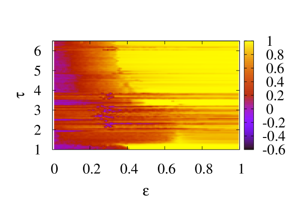
Figure 9: (color online) CPS regime in the parameter space $(\varepsilon,\tau)$ characterized using the values of the index $C_{CPR}$.

The largest ten Lyapunov exponents of the coupled time-delay systems for the delay time $\tau=6.0$ are shown in Fig. 8(a) in the range of $\varepsilon\in(0,1)$. The four positive Lyapunov exponents of the drive system continue to remain positive in the entire range of $\varepsilon$. The three least positive Lyapunov exponents of the response system become gradually negative for $\varepsilon>0.4$ and the largest positive Lyapunov exponent becomes negative for $\varepsilon>0.5$, at which $C_{CPR}$ [Fig. 8(b)] also reaches the value of unity, indicating the existence of high quality CPS in the hyperchaotic regime. Further, we have scanned the $(\varepsilon,\tau)$ parameter space by calculating the value of $C_{CPR}$ to demarcate the regimes of CPS as depicted in Fig. 9. As discussed above, the coupled systems are in CPS when the value of $C_{CPR}$$\approx 1$ and it is evident from this figure that CPS occurs in a wide range of $\tau$.

To summarize, we have demonstrated the notion of CPS in a unidirectionally coupled time-delay electronic circuit with threshold nonlinearity in both chaotic and hyperchaotic regimes. The existence of CPS is observed experimentally from snapshots of the time evolution of both the coupled systems and is confirmed with the framework of localized sets. Further we have corroborated the synchronization transition numerically using the phase differences, the concept of localized sets, changes in the largest Lyapunov exponents and from the values of $C_{CPR}$ of the coupled time-delay systems, which agree well with the experimental observations. We strongly believe that our results especially with the framework of localized sets will lead to the identification of CPS in other physical systems with delay and to their potential applications.

D. V. S has been supported by the Alexander von Humboldt Foundation. The work of K. S. and M. L. has been supported by the Department of Science and Technology (DST), Government of India sponsored IRHPA research project, INSA senior scientist program, and DST Ramanna program of M. L. J. K. acknowledges the support from EU under project No. 240763 PHOCUS(FP7-ICT-2009-C).

References

- Pikovsky et al. (2001) A. S. Pikovsky, M. G. Rosenblum, and J. Kurths, Synchronization - A Unified Approach to Nonlinear Science (Cambridge University Press, Cambridge, 2001).
- Boccaletti et al. (2002) S. Boccaletti, J. Kurths, G. Osipov, D. L. Valladares, and C. S. Zhou, Phys. Rep. 366, 1 (2002).
- Scannel et al. (1999) J. W. Scannell et. al., Cereb. Cortex. 9, 277 (1999).
- Varela et al. (1998) C. Schäfer, M. G. Rosenblum, J. Kurths, and H. H. Abel, Nature 392, 239 (1998).
- Varela et al. (1999) B. Blasius, A. Huppert, and L. Stone, Nature 399, 354 (1999).
- Grenfell et al. (2001) B. T. Grenfell et. al., Nature (London) 414, 716 (2001).
- RosaJr. et al. (2003) E. Rosa et. al., Phys. Rev. E 68, 025202(R) (2003); M. S. Baptista et. al., Phys. Rev. E 67, 056212 (2003).
- Volodehenko et al. (2001) K. V. Volodehenko et. al., Opt. Lett. 26, 1406 (2001); D. J. DeShazer et. al., Phys. Rev. Lett. 87, 044101 (2001).
- Maza et al. (2000) D. Maza, A. Vallone, H. Mancini, and S. Boccaletti, Phys. Rev. Lett. 85, 5567 (2000).
- Tass et al. (1998) P. Tass et. al., Phys. Rev. Lett. 81, 3291 (1998); R. C. Elson et. al., Phys. Rev. Lett. 81, 5692 (1998).
- Maraun and Kurths (2005) D. Maraun and J. Kurths, Geophys. Res. Lett. 32, L15709 (2005).
- Vicent et al. (1998) P. Vicent et. al., Phys. Rev. E 70, 046216 (2004).
- Senthil2 et al. (2006) D. V. Senthilkumar, M. Lakshmanan, and J. Kurths, Phys. Rev. E 74, 035205(R) (2006); Chaos 18, 023118 (2008); Eur. Phys. J. Special Topics 164, 35 (2008).
- Suresh et al. (2010) R. Suresh, D. V. Senthilkumar, M. Lakshmanan, and J. Kurths, Phys. Rev. E 82, 016215 (2010).
- Pereira et al. (2007) T. Pereira, M. S. Baptista, and J. Kurths, Phys. Rev. E 75, 026216 (2007).
- Marwan et al. (2007) N. Marwan, M. C. Romano, M. Thiel, and J. Kurths, Phys. Rep. 438, 237 (2007).
- Srinivasan et al. (2007) K. Srinivasan et. al., Int. J. Bifurcation and Chaos 21, (2011)(To appear); arXiv:1008.4011.
- Srinivasan et al. (2007) K. Srinivasan, D. V. Senthilkumar, K. Murali, M. Lakshmanan, and J. Kurths, (submitted); arXiv:1008.3300.