Quantum controlled phase gate based on two nonresonant quantum dots trapped in two coupled photonic crystal cavities

Abstract

We propose a scheme for realizing two-qubit quantum phase gates with two nonidentical quantum dots trapped in two coupled photonic crystal cavities and driven by classical laser fields. During the gate operation, neither the cavity modes nor the quantum dots are excited. The system can acquire different phases conditional upon the different states of the quantum dots, which can be used to realize the controlled phase gate.

I Introduction

In recent years, there are great advancements on constructing the basic components of quantum information processing (QIP) devices both in experiments and theories 01 . As the cavity quantum electrodynamics (CQED) can manipulate the qubits efficiently, it has been become one of the most promising approaches to realize the QIP devices 02 ; 03 . Although the qubits in CQED can be atoms 03 , ions 05 ; 06 , or quantum dots (QDs) 07 , the demonstrations of such basic building blocks of the quantum on-chip network have relied on the atomic systems 08 ; 09 ; 10 . Furthermore, a solid state implementation of these pioneering approaches would open new opportunities for scaling the network into practical and useful QIP systems 01 . Among the proposed schemes based on solid quantum devices, the systems of self-assembled QDs embedded in photonic crystal (PC) nanocavities have been a kind of very promising systems. That is not just because the strong QD-cavity interaction can be realized in these systems 11 ; 12 ; 13 , but also because both QDs and PC cavities are suitable for monolithic on-chip integration.

However, there are two main challenges in this kind of systems. One is that the variation in emission frequencies of the self-assembled QDs is large 14 , the other is that the interaction between the QDs is difficult to control 15 . So far, there are several methods which have been used to bring the emission frequencies of nonidentical QDs into the same, such as, by using Stark shift tuning 16 and voltage tuning 17 . There are also several solutions which have been used to control the interaction between QDs, for instance, coherent manipulating coupled QDs 15 , and controlling the coupled QDs by Kondo effect 18 . In experiments, the tuning of individual QD frequencies has been achieved for two closely spaced QDs in a PC cavity 17 . However, there are few schemes about how to achieve the controlled interaction and the controlled gate with the QDs trapped in two coupled cavities.

Recently, Zheng proposed a scheme for implementing quantum gates by using two atoms trapped in distant cavities connected by an optical fiber 241 . But his proposal is based on two identical atoms, and there is no directly coupling between the cavities. Motivated by this work, we propose a scheme for realizing the controlled phase gate with two different QDs trapped in two directly coupled PC cavities. The advantages of our scheme are as follows. Firstly, it could be controlled by the external light fields. Secondly, it can be realized in the case of large variation in emission frequencies of the QDs. Thirdly, there is no cavity photon population involved and the QDs are always in their ground states. Moreover, our scheme does not require the condition that the coupling between QD and cavity is smaller than that between cavities.

The organization of this paper is as follows. In Sec. II, we introduce the theoretical model and Hamiltonian. In Sec. III, we present the derivation of effective Hamiltonian. In Sec. IV, we show the controlled phase gate. The discussion and conclusion is given in Sec. V.

II Theoretical Model and Hamiltonian

We consider that two charged GaAs/AlGaAs QDs are placed in two coupled single-mode PC cavities, which have the same frequency. Each dot has two lower states $|g\rangle=|\uparrow\rangle$, $|f\rangle=|\downarrow\rangle$ and a higher state $|e\rangle=|\uparrow\downarrow\Uparrow\rangle$, here ($|\uparrow\rangle$, $|\downarrow\rangle$) and ($|\Uparrow\rangle$, $|\Downarrow\rangle$) denote the spin up and spin down for electron and hole, respectively. The transitions $|g\rangle\leftrightarrow|e\rangle$ and $|f\rangle\leftrightarrow|e\rangle$ are coupled to the vertical polarization and horizontal polarization lights, respectively. Choosing the fields with the vertical polarization, the state $|f\rangle$ is not affected during the interactions, and only the transition $|g\rangle$ $\leftrightarrow$ $|e\rangle$ is coupled to the cavity mode and classical laser field 35 . Then the Hamiltonian for this model can be written as:

$$\begin{array}[]{rcl}\hat{H}&=&\sum\limits_{j=A,B}(g_{j}a_{j}e^{i\Delta_{j}^{C}t}+\Omega_{j}e^{i\Delta_{j}t})\sigma_{j}^{+}+\nu a_{A}^{+}a_{B}+H.c.\end{array}$$ (1)

where$\ \sigma_{j}^{+}=|e\rangle_{j}\langle g|$, $g_{j}$ is the coupling constant between the cavity $j$ and QD $j$, $\Omega_{j}$ are the Rabi frequencies of the laser fields, the detunings are $\Delta_{j}^{C}$, and $\Delta_{j}$, respectively, $a_{j}^{{\dagger}}$ and $a_{j}$ are the creation and annihilation operators for the $j$th cavity mode, $\nu$ is the coupling strength between the two cavity modes (see FIG.1 ).

III Derivation of effective Hamiltonian

Introducing new annihilation operators $c_{1}$ and $c_{2}$, and defining $a_{A}=\frac{1}{\sqrt{2}}(c_{1}+c_{2})$, $a_{B}=\frac{1}{\sqrt{2}}(c_{2}-c_{1})$, and $\Delta_{j}^{C}=\Delta_{j}+\delta$, the Hamiltonian can be rewritten as

$$\begin{array}[]{rcl}\hat{H}_{int}&=&\hat{H}_{0}+\hat{H}_{i}\\ \hat{H}_{0}&=&\nu(c_{2}^{+}c_{2}-c_{1}^{+}c_{1}),\\ \hat{H}_{i}&=&\sum\limits_{j=A,B}[\frac{1}{2}g_{j}(c_{1}+c_{2})e^{i(\Delta_{j}+\delta)t}+\Omega_{j}e^{i\Delta_{j}t}]\sigma_{j}^{+}\\ &+&H.c.\end{array}$$ (2)

With the application of the unitary transformation $e^{iH_{0}t}$, the Hamiltonian takes the form:

$$\begin{array}[]{rcl}\hat{H}_{I}&=&[\frac{1}{2}g_{A}(c_{2}e^{i(\Delta_{A}+\delta-\nu)t}+c_{1}e^{i(\Delta_{A}+\delta+\nu)t})+\Omega_{A}e^{i\Delta_{A}t}]\sigma_{A}^{+}\\ &+&[\frac{1}{2}g_{B}(c_{2}e^{i(\Delta_{B}+\delta-\nu)t}-c_{1}e^{i(\Delta_{B}+\delta+\nu)t})+\Omega_{B}e^{i\Delta_{B}t}]\sigma_{B}^{+}\\ &+&H.c.\end{array}$$ (3)

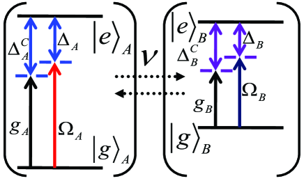
Figure 1: Schematic diagram of the system. Each dot is trapped in its corresponding cavity and driven by a light field. Photons can hop between the cavities.

Now, we will use the method proposed in Ref. 24 ; 28 to derive the effective Hamiltonian for this system. With $|\Delta_{j}|,|\Delta_{j}^{{}^{\prime}}|\gg\nu,\delta,|g_{j}|,|\Omega_{j}|$ assumed, the probability for QDs absorbing photons from the light field and being excited will be ignored, and the excited state of QD can be adiabatically eliminated. Thus we can obtain the effective Hamiltonian:

$$\begin{array}[]{rcl}\hat{H}_{eff-1}&=&-c_{2}(\lambda_{A,2}\sigma_{A}^{-}\sigma_{A}^{+}-\lambda_{B,2}\sigma_{B}^{-}\sigma_{B}^{+})e^{i(\delta-\nu)t}\\ &-&c_{1}(\lambda_{A,1}\sigma_{A}^{-}\sigma_{A}^{+}+\lambda_{B,1}\sigma_{B}^{-}\sigma_{B}^{+})e^{i(\delta+\nu)t}\\ &-&(k_{A}\sigma_{A}^{-}\sigma_{A}^{+}-k_{B}\sigma_{B}^{-}\sigma_{B}^{+})c_{1}c_{2}^{+}\sigma_{A}^{-}\sigma_{A}^{+}e^{-i2vt}\\ &+&H.c.\\ &-&(l_{A,1}c_{1}^{+}c_{1}+l_{A,2}c_{2}^{+}c_{2}+l_{A,3})\sigma_{A}^{-}\sigma_{A}^{+}\\ &-&(l_{B,1}c_{1}^{+}c_{1}+l_{B,2}c_{2}^{+}c_{2}+l_{B,3})\sigma_{B}^{-}\sigma_{B}^{+}.\end{array}$$ (4)

where

$$\begin{array}[]{l}\lambda_{j,1}=\dfrac{g_{j}\Omega_{j}^{\ast}}{4}(\frac{1}{\Delta_{j}+\delta+\nu}+\frac{1}{\Delta_{j}});\\ \lambda_{j,2}=\dfrac{g_{j}\Omega_{j}^{\ast}}{4}(\frac{1}{\Delta_{j}+\delta-\nu}+\frac{1}{\Delta_{j}});\\ k_{j}=\dfrac{|g_{j}|^{2}}{8}(\frac{1}{\Delta_{j}+\delta+\nu}+\frac{1}{\Delta_{j}+\delta-\nu});\\ l_{j,1}=\frac{|g_{j}|^{2}}{4(\Delta_{j}+\delta-\nu)};l_{j,2}=\frac{|g_{j}|^{2}}{4(\Delta_{j}+\delta+\nu)};\\ l_{j,3}=\frac{|\Omega_{j}|^{2}}{\Delta_{j}};\Delta_{1}=\delta-\nu;\Delta_{2}=\delta+\nu.\end{array}$$

Under the condition $\delta+\nu,\delta-\nu,2v\gg\lambda_{j,1},\lambda_{j,2},k_{j}$, the new bosonic modes cannot exchange energy with each other and with the classical fields, the coupling between the two cavities can be much larger than the one between QD and cavity. Moreover, the couplings between the bosonic modes and the classical fields lead to energy shifts which are only depending upon the number of QDs in the state $|g\rangle$, while the couplings between different bosonic modes cause energy shifts depending upon both the excitation numbers of the modes and the number of QDs in the state $|g\rangle$. Then the effective Hamiltonian takes the form:

$$\begin{array}[]{rcl}\hat{H}_{eff-2}&=&\frac{1}{\delta-\nu}(\lambda_{A,2}\sigma_{A}^{-}\sigma_{A}^{+}-\lambda_{B,2}\sigma_{B}^{-}\sigma_{B}^{+})\\ &\ast&(\lambda_{A,2}^{\ast}\sigma_{A}^{-}\sigma_{A}^{+}-\lambda_{B,2}^{\ast}\sigma_{B}^{-}\sigma_{B}^{+})\\ &+&\frac{1}{\delta+\nu}(\lambda_{A,1}\sigma_{A}^{-}\sigma_{A}^{+}+\lambda_{B,1}\sigma_{B}^{-}\sigma_{B}^{+})\\ &\ast&(\lambda_{A,1}^{\ast}\sigma_{A}^{-}\sigma_{A}^{+}+\lambda_{B,1}^{\ast}\sigma_{B}^{-}\sigma_{B}^{+})\\ &+&\frac{1}{2v}(k_{A}\sigma_{A}^{-}\sigma_{A}^{+}-k_{B}\sigma_{B}^{-}\sigma_{B}^{+})^{2}(c_{1}^{+}c_{1}-c_{2}^{+}c_{2})\\ &-&(l_{A,1}c_{1}^{+}c_{1}+l_{A,2}c_{2}^{+}c_{2}+l_{A,3})\sigma_{A}^{-}\sigma_{A}^{+}\\ &-&(l_{B,1}c_{1}^{+}c_{1}+l_{B,2}c_{2}^{+}c_{2}+l_{B,3})\sigma_{B}^{-}\sigma_{B}^{+}.\end{array}$$ (5)

It shows, during the interaction, the excitation numbers of the bosonic modes $c_{1}$ and $c_{2}$ are conserved, so does the one for the cavity modes. Assume that the initial state for two cavity modes is in the vacuum state, the new bosonic modes will be in the vacuum state during the evolution. In this situation, the effective Hamiltonian reduces to

$$\begin{array}[]{rcl}\hat{H}_{eff}&=&\frac{1}{\delta-\nu}(\lambda_{A,2}\sigma_{A}^{-}\sigma_{A}^{+}-\lambda_{B,2}\sigma_{B}^{-}\sigma_{B}^{+})\\ &\ast&(\lambda_{A,2}^{\ast}\sigma_{A}^{-}\sigma_{A}^{+}-\lambda_{B,2}^{\ast}\sigma_{B}^{-}\sigma_{B}^{+})\\ &+&\frac{1}{\delta+\nu}(\lambda_{A,1}\sigma_{A}^{-}\sigma_{A}^{+}+\lambda_{B,1}\sigma_{B}^{-}\sigma_{B}^{+})\\ &\ast&(\lambda_{A,1}^{\ast}\sigma_{A}^{-}\sigma_{A}^{+}+\lambda_{B,1}^{\ast}\sigma_{B}^{-}\sigma_{B}^{+})\\ &-&l_{A,3}\sigma_{A}^{-}\sigma_{A}^{+}-l_{B,3}\sigma_{B}^{-}\sigma_{B}^{+}.\end{array}$$ (6)

This equation can be understood as follows. With the laser field acting, QDs will take place the Stark shifts and acquire the virtual excitation, and the virtual excitation will induce the coupling between the vacuum bosonic modes and classical fields. As the Stark shifts are nonlinear in the number of the QDs in the state $|g\rangle$, the system can acquire a phase conditional upon the number of the QDs in the state $|g\rangle$.

IV The Controlled Phase gate

Now, we will show how to construct the controlled phase gate in this system. First of all, the inforamtion of the system is encoded in the states $|g\rangle$ and $|f\rangle$. Then, according to the effective Hamiltonian (6), the evolution for states {$|ff\rangle$, $|fg\rangle$, $|gf\rangle$, and $|gg\rangle$} can be written as:

$$\left\{\begin{array}[]{rcl}|ff\rangle&\rightarrow&|ff\rangle,\\ |fg\rangle&\rightarrow&e^{-i\Phi_{A}t}|fg\rangle,\\ |gf\rangle&\rightarrow&e^{-i\Phi_{B}t}|gf\rangle,\\ |gg\rangle&\rightarrow&e^{-i(\Phi_{A}+\Phi_{B}+\eta)t}|gg\rangle.\end{array}\right.$$ (7)

where

$$\left\{\begin{array}[]{rcl}\Phi_{A}&=&\frac{|\lambda_{A,2}|^{2}}{\delta-\nu}+\frac{|\lambda_{A,1}|^{2}}{\delta+\nu}-l_{A,3},\\ \Phi_{B}&=&\frac{|\lambda_{B,2}|^{2}}{\delta-\nu}+\frac{|\lambda_{B,1}|^{2}}{\delta+\nu}-l_{B,3},\\ \eta&=&\frac{1}{\delta+\nu}(\lambda_{A,1}\lambda_{B,1}^{\ast}+\lambda_{A,1}^{\ast}\lambda_{B,1})\\ &-&\frac{1}{\delta-\nu}(\lambda_{A,2}\lambda_{B,2}^{\ast}+\lambda_{A,2}^{\ast}\lambda_{B,2}).\\ &=&2(\frac{|\lambda_{A,1}\lambda_{B,1}|\cos\theta_{1}}{\delta+\nu}+\frac{|\lambda_{A,2}\lambda_{B,2}|\cos\theta_{2}}{v-\delta}),\end{array}\right.$$ (8)

$\theta_{1}$ and $\theta_{2}$ are the arguments of $\lambda_{A,1}\lambda_{B,1}^{\ast}$ and $\lambda_{A,2}\lambda_{B,2}^{\ast}$, respectively.

With the application of single-qubit operations29

$$\left\{\begin{array}[]{rcl}|g_{A}\rangle&\rightarrow&e^{i\Phi_{A}t}|g_{A}\rangle,\\ |g_{B}\rangle&\rightarrow&e^{i\Phi_{B}t}|g_{B}\rangle,\end{array}\right.$$ (9)

Eq.(7) will transform into

$$\left\{\begin{array}[]{rcl}|ff\rangle&\rightarrow&|ff\rangle,\\ |fg\rangle&\rightarrow&|fg\rangle,\\ |gf\rangle&\rightarrow&|gf\rangle,\\ |gg\rangle&\rightarrow&e^{-i\eta t}|gg\rangle.\end{array}\right.$$ (10)

It is clearly, with the choice of $\eta t=\pi$, this transformation corresponds to the quantum controlled phase $\pi$ gate operation, in which if and only if both controlling and controlled qubits are in the states $|g\rangle$, there will be an additional phase $\pi$ in the system.

V Discussion and Conclusion

In order to confirm the validity of the proposal, we takes controlled phase $\pi$ gate (C-Z gate) as an example to disscuss the realizability in the experiment. According to experimentally achievable parameters in the system of QDs embedded in a single-mode cavity 35 ; 36 , the coupling constant between cavity and QD is $g\sim 0.1meV$, the decay time for cavity is $\tau_{c}\sim 1ns$, and the energy relaxation time of the excited state is $\tau_{e}\sim 1.4ns$. With the choices of the coupling constants and detunings as follows: $g_{A}=0.1meV$, $g_{B}=0.08meV$, $\Omega_{A}=10meV$, $\Omega_{B}=13.75meV$, $\Delta_{A}=200meV$, $\Delta_{B}=220meV$, $\delta=2g_{A}$, $\nu=12g_{A}$, we have $\lambda_{j,1}\simeq\lambda_{j,2}\sim 0.0025meV$, which satisfy the approximation conditions mentioned above. The calculations show that i) the max-occupation probability of the excited state is $\max(P_{e})\sim 1/256(\simeq\max[\Omega_{j}^{2}/\Delta_{j}^{2}])$, and thus, the effective energy relaxation time is $t_{e}\sim 358ns(\simeq\tau_{e}/P_{e})$. ii) the occupation probability of the photon is $P_{c}\sim 1/900(\simeq\max[\lambda_{j,1}^{2},\lambda_{j,2}^{2}]/\delta^{2})$, so the effective decay time is $t_{c}\sim 900ns(\simeq\tau_{c}/P_{c})$, iii) the required effective interaction time for the C-Z gate is $t\sim 50ns(\simeq\pi/(2\epsilon))$. Therefore, it is possible to perform several C-Z gates within the decoherence time $\min[t_{e},t_{c}]\sim 358ns$.

In summary, we have shown a protocol that two nonidentical QDs trapped in two coupled PC cavities can be used to construct the two-qubit controlled phase gate with the application of the classical light fields. During the gate operation, none of the QDs is in the excited state, and both of the cavities are in the vacuum state. The distinct advantages of the proposed scheme are as follows: firstly, it is controllable; secondly, during the gate operation, there is no cavity photon population involved and the QDs are always in their ground states; finally, as the QDs are non-identical and the coupling between the two cavities can be much larger than the one between QD and cavity, it is more practical. Therefore, we can use this scheme to construct a kind of solid-state controllable quantum logical devices. In addition, as the controlled phase gate is a universal gate, this system can also realize the controlled entanglement and interaction between the two nonidentical QDs trapped in two coupled cavities.

References

• (1) D. Englund, A. Faraon, I. Fushman , B. Ellis and J. Vučković, Single Semiconductor Quantum Dots, edited by P. Michler (Springer Berlin Heidelberg, 2009).
• (2) J. I. Cirac, P. Zoller, H. J. Kimble, H. Mabuchi, Phys. Rev. Lett 78. 3221 (1997)
• (3) L. M. Duan, H. J. Kimble, Phys. Rev. Lett 92, 127902 (2004).
• (4) C. Monroe, D. M. Meekhof, B. E. King, W. M. Itano, D. J. Wineland, Phys. Rev. Lett 75, 4714 (1995)
• (5) J. Chiaverini, D. Leibfried, T. Schaetz, M. D. Barrett, R. B. Blakestad, J. Britton, W. M. Itano, J. D. Jost, E. Knill, C. Langer, R. Ozeri, D.J. Wineland, Nature 432, 602 (2005)
• (6) A. Imamoglu, D. D. Awschalom, G. Burkard, D.P. DiVincenzo, D. Loss, m. Sherwin, A. Small, Phys. Rev. Lett 83, 4204 (1999)
• (7) Q. Turchette, C. Hood, W. Lange, H. Mabuchi, H.J. Kimble, Phys. Rev. Lett 75, 4710 (1995)
• (8) K. M. Birnbaum, A. Boca, R. Miller, A.D. Boozer, T.E. Northup, H.J. Kimble, Nature 436, 87 (2005)
• (9) G. Nogues, A. Rauschenbeutel, S. Osnaghi, M. Brune, J. M. Raimond, S. Haroche, Nature 400, 239 (1999)
• (10) D. Englund, D. Fattal, E. Waks, G. Solomon, B. Zhang, T. Nakaoka, Y. Arakawa, Y. Yamamoto, and J. Vukovi, Phys. Rev. Lett 95, 013904 (2005).
• (11) T. Yoshie, A. Scherer, J. Hendrickson, G. Khitrova, H. M. Gibbs, G. Rupper, C. Ell, O. B. Shchekin, and D. G. Deppe, Nature, 432, 200 (2004)
• (12) K. Hennessy, A. Badolato, M. Winger, D. Gerace, M. Atature, S. Gulde, S. Falt, E.L. Hu, A. Imamoglu, Nature, 445, 896 (2007)
• (13) A. Imamoğlu, S. Falt, J. Dreiser, G. Fernandez, M. Atature, K. Hennessy, A. Badolato, and D. Gerace, J. Appl. Phys. 101, 081602 (2007) .
• (14) J. R. Petta, A. C. Johnson, J. M. Taylor, E. A. Laird, A. Yacoby, M. D. Lukin, C. M. Marcus, M. P. Hanson, and A. C. Gossard, Science, 309, 2180 (2005)
• (15) A. Nazir, B. W. Lovett, G. Andrew and D. Briggs, Phys. Rev. A 70, 052301 (2004); J. Q. Zhang, L. L. Xu, and Z. M. Zhang, Phys. Lett. A, 374, 3818 (2010).
• (16) H. Kim, S. M. Thon, P. M. Petroff, and D. Bouwmeester, Appl. Phys. Lett. 95, 243107 (2009)
• (17) N. J. Craig, J. M. Taylor, E. A. Lester, C. M. Marcus, M. P. Hanson, A. C. Gossard, Science 304, 565 (2004)
• (18) S. B. Zheng, Appl. Phys. Lett. 94, 154101 (2009)
• (19) X. Xu, Y. Wu, B. Sun, Q. Huang, J. Cheng, D. G. Steel, A. S. Bracker, D. Gammon, C. Emary, and L. J. Sham Phys. Rev. Lett 99, 097401 (2007)
• (20) X. L. Feng, C. F. Wu, H. Sun, and C. H. Oh, Phys. Rev. Lett 103, 200501 (2009)
• (21) D. F. V. James, and J. Jerke, Can. J. Phys. 85, 325 (2007)
• (22) I. Fushman, D. Englund, A. Faraon, N. Stoltz, P. Petroff, J. Vuckovic, Science 320, 769 (2008)
• (23) P. Yao, and S. Hughes, Optics Express, 17, 11505-11514 (2009); A. Laucht, A. Neumann, J. M. Villas-Boas, M. Bichler, M.-C. Amann, and J. J. Finley Phys.Rev.B 77, 161303 (2008); M. Atature, J. Dreiser, A Badolato, Al. Hogele, K. Karrai, and A. Imamoglu, Science 312 551-553 (2006).