Analysis of the radiative thermal transfer in planar multi-layer systems with various emissivity and transmissivity properties

Abstract

Abstract The paper analyzes the radiative thermal transfer in a liquid helium cryostat with liquid nitrogen shielding. A infinite plane walls model is used for demonstrating a method for lowering the radiative heat transfer and the numerical results for two such systems are presented. Some advantages concerning the opportunity of using semi-transparent walls are analytically and numerically demonstrated.

Keywords: Radiative heat transfer, emissivity, thermal shield, cryostat

I Introduction

In a previous paper ssarxiv4 the thermal conductive flux in a cryostat was analyzed, and some methods for its reduction were suggested. In this paper we analyze the other major process of heat transfer which occurs in the same system, the radiative heat transfer. The classical method for lowering the values of this flux involves a number of reflective screens interposed in the vacuum chamber between the hot and the cold wall sieg , as in figure 1.

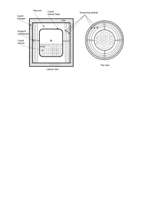
Figure 1: The system of two infinite planes in vacuum

The net radiative thermal flux from the warm wall to the cold one is strongly dependent on the properties of the walls and shields, especially their emissivity hprs , emis . Although these properties are not entirely known for cryogenic temperatures and have to be experimentally determined, some theoretical consideration concerning the general relationships describing the radiative thermal transfer may be drawn and they allow the proper design for improved cryostats.

We analyze in the following the basic relationships for calculating this process, and a method for significantly reducing it is presented.

II Radiative heat transfer between reflective infinite planes in vacuum

Let us consider the system composed by two plane surfaces ${S_{a}}$ and ${S_{b}}$ placed in vacuum as in figure 2 in steady state conditions at temperatures ${T_{a}}$ and ${T_{b}}$.

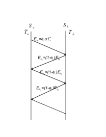
Figure 2: The system of two infinite planes in vacuum

We analyze the radiative thermal flux between the two surfaces, from ${S_{a}}$ to ${S_{b}}$ if the first one is in contact with liquid nitrogen at the temperature ${T_{a}}=77.36\rm K$ and the second one is in contact with liquid helium at the temperature ${T_{b}}=4.22\rm K$.

The thermal flux emitted by the surface unit by ${S_{a}}$, if it presents the emissivity ${e_{1}}$ considered constant with the temperature is (figure 2):

$${E_{{a_{1}}}}={e_{1}}\sigma T_{a}^{4}$$ (1)

conforming to the Stephan-Boltzmann law, with the constant landau $\sigma=\frac{{2{\pi^{2}}k_{B}^{4}}}{{15{h^{3}}{c^{2}}}}=5,6692\cdot{10^{-8}}\rm W/({m^{2}}{K^{4}})$

This thermal flux is partially reflected by the surface ${S_{b}}$, so that a fraction of it is returned to the surface ${S_{a}}$. According to Kirchhoff law, the reflexivity $r$ of the surface is $r=1-e$, so that this fraction is chis

$${E_{b1}}=(1-{e_{2}}){E_{a1}}={e_{1}}(1-{e_{2}})\sigma T_{a}^{4}$$ (2)

This flux is again reflected to ${S_{a}}$,as a secondary flux ${E_{{a_{2}}}}$.

$${E_{{a_{2}}}}=(1-{e_{1}}){E_{{b_{1}}}}={e_{1}}(1-{e_{1}})(1-{e_{2}})\sigma T_{a}^{4}$$ (3)

After other two reflections the surface ${S_{a}}$ transmits also the flux:

$${E_{{a_{3}}}}={e_{1}}{(1-{e_{1}})^{2}}{(1-{e_{2}})^{2}}\sigma T_{a}^{4}$$ (4)

and after $k$ double reflections the flux is:

$${E_{{a_{k}}}}={e_{1}}{(1-{e_{1}})^{(k-1)}}{(1-{e_{2}})^{(k-1)}}T_{a}^{4}$$ (5)

It follows that the total flux ${E_{0}}$ emitted by ${S_{a}}$ and incident on ${S_{b}}$ is:

$$\begin{gathered}{E_{a}}={E_{a1}}+{E_{a2}}+...+{E_{ak}}+...={e_{1}}\sigma T_{a}^{4}+{e_{1}}(1-{e_{1}})(1-{e_{2}})\sigma T_{a}^{4}\hfill\\ +{e_{1}}{(1-{e_{1}})^{2}}{(1-{e_{2}})^{2}}\sigma T_{a}^{4}+...+{e_{1}}{(1-{e_{1}})^{k-1}}{(1-{e_{2}})^{k-1}}\sigma T_{a}^{4}+...\hfill\\ \end{gathered}$$ (6)

$${E_{a}}={e_{1}}\sigma T_{a}^{4}\frac{1}{{1-(1-{e_{1}})(1-{e_{2}})}}$$ (7)

The total flux ${E_{ab}}$ emitted by ${S_{a}}$ and absorbed by ${S_{b}}$ is:

$${E_{ab}}={e_{2}}{E_{a}}={e_{2}}{e_{1}}\sigma T_{a}^{4}\frac{1}{{1-(1-{e_{1}})(1-{e_{2}})}}$$ (8)

For calculating the net flux flowing from the wall ${S_{a}}$ to the wall ${S_{b}}$ we must subtract the flux emitted by ${S_{b}}$ and absorbed by ${S_{a}}$ (as in figure 3). At the temperature ${T_{b}}$ this flux has an expression similar with (8):

$${E_{ba}}=\frac{{{e_{1}}{e_{2}}\sigma T_{b}^{4}}}{{1-(1-{e_{1}})(1-{e_{2}})}}$$ (9)

If ${T_{a}}>{T_{b}}$, the thermal flux emitted by ${S_{a}}$ is greater than that emitted by ${S_{b}}$, and the total net thermal flux from ${S_{a}}$ to ${S_{b}}$ is:

$$E={E_{ab}}-{E_{ba}}$$ (10)

$$E=\frac{1}{{\frac{1}{{{e_{1}}}}+\frac{1}{{{e_{2}}}}-1}}\sigma(T_{a}^{4}-T_{b}^{4})$$ (11)

In the case that the walls have the same emissivity ${e_{1}}={e_{2}}=e$:

$$E=\frac{e}{{2-e}}\sigma(T_{a}^{4}-T_{b}^{4})$$ (12)

For calculating the net thermal flux the emissivity coefficients ${e_{1}}$ and ${e_{2}}$ and the temperatures are necessary. If the temperature ${T_{b}}$ is not given, it may be calculated taking into consideration that if ${S_{b}}$ is placed in vacuum in steady state conditions the thermal flux absorbed is equal with the emitted one. So, imposing a value for the total net flux through the surface ${S_{b}}$,its temperature is:

$${T_{b}}={\left[{T_{a}^{4}-\frac{E}{\sigma}\left({\frac{1}{{{e_{1}}}}+\frac{1}{{{e_{2}}}}-1}\right)}\right]^{\frac{1}{4}}}$$ (13)

In the case that between the two walls there is a third wall with the left side emissivity $e_{2s}$ and the right side emissivity $e_{2d}$ (as in figure 3), for calculating the thermal flux we have to consider the condition that in steady state regime the thermal flux emitted by ${S_{a}}$ and absorbed by ${S_{b}}$ is equal to the flux emitted by ${S_{b}}$ and absorbed by ${S_{c}}$. We obtain the equations

$$\left\{\begin{gathered}E=\frac{1}{{\frac{1}{{{e_{1d}}}}+\frac{1}{{{e_{2s}}}}-1}}\sigma(T_{a}^{4}-T_{b}^{4})\hfill\\ E=\frac{1}{{\frac{1}{{{e_{2d}}}}+\frac{1}{{{e_{3s}}}}-1}}\sigma(T_{b}^{4}-T_{c}^{4})\hfill\\ \end{gathered}\right.$$ (14)

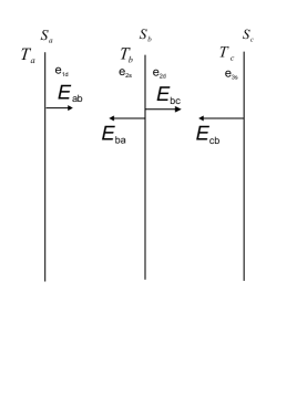
Figure 3: The system of two infinite planes in vacuum

If the exterior walls temperatures ${T_{a}}$ and ${T_{c}}$ are known, by solving this system we obtain the unknowns $E$ and ${T_{b}}$

$$E=\frac{1}{{\frac{1}{{{e_{1d}}}}+\frac{1}{{{e_{2s}}}}+\frac{1}{{{e_{2d}}}}+\frac{1}{{{e_{3s}}}}-2}}\sigma(T_{a}^{4}-T_{c}^{4})$$ (15)

$${T_{b}}={\left[{\frac{{\left({\frac{1}{{{e_{3s}}}}+\frac{1}{{{e_{2d}}}}-1}\right)T_{a}^{4}+\left({\frac{1}{{e2}}+\frac{1}{{{e_{1d}}}}-1}\right)T_{c}^{4}}}{{\frac{1}{{{e_{3s}}}}+\frac{1}{{{e_{2s}}}}+\frac{1}{{{e_{1d}}}}+\frac{1}{{{e_{2d}}}}-2}}}\right]^{\frac{1}{4}}}$$ (16)

In the case that all the surfaces have the same emissivity ${e_{1d}}={e_{2s}}={e_{2d}}={e_{3s}}=e$, the expressions simplify as

$$E=\frac{e}{{2(2-e)}}\sigma(T_{a}^{4}-T_{c}^{4})$$ (17)

$${T_{b}}={\left({\frac{{T_{a}^{4}+T_{c}^{4}}}{2}}\right)^{\frac{1}{4}}}$$ (18)

One may notice that the thermal flux is twice smaller that in the case of two walls, and the fourth power of middle wall temperature is the average value of the exterior temperature at the fourth power.

Generalizing, for the case of $n$ walls with the same emissivity $e$, and with the extreme temperatures $T_{1}$ and $T_{2}$, the total net flux transmitted from the warmest wall and absorbed by the coldest one is

$$E=\frac{e}{{(n-1)(2-e)}}\sigma(T_{1}^{4}-T_{n}^{4})$$ (19)

and the intermediate walls temperatures $T_{k}$ are

$${T_{k}}={\left\{{\frac{1}{n-1}[(n-k)T_{1}^{4}+(k-1)T_{n}^{4}]}\right\}^{\frac{1}{4}}},\quad k=2,3,...,n-1$$ (20)

In the table 1 we present numerical results for the radiative heat transfer between two plane infinite walls with different emissivity coefficients. One may notice that the minimum radiative heat transfer is obtained for the lowest values of the emissivity of both walls, as expected. These numerical results may be used as a reference for more sophisticated methods for reducing the thermal flux, as it will be presented further. For a system of $n$ walls with the same emissivity, the corresponding value on the diagonal should be divided by $n-1$.

Table 1: The heat transfer power reported to the surface between two plane walls, for various values of the emissivity of the right side and the left side ($\rm W/m^{2}$).

${}_{e_{l}}\backslash^{e_{r}}$	0.1	0.2	0.3	0.4	0.5	0.6	0.7	0.8	0.9
0.1	0.105	0.142	0.162	0.173	0.181	0.187	0.191	0.194	0.197
0.2	0.142	0.221	0.272	0.307	0.332	0.352	0.367	0.38	0.39
0.3	0.162	0.272	0.352	0.412	0.46	0.498	0.53	0.556	0.579
0.4	0.173	0.307	0.412	0.498	0.569	0.629	0.68	0.725	0.763
0.5	0.181	0.332	0.46	0.569	0.664	0.747	0.821	0.886	0.944
0.6	0.187	0.352	0.498	0.629	0.747	0.854	0.951	1.04	1.121
0.7	0.191	0.367	0.53	0.68	0.821	0.951	1.073	1.187	1.294
0.8	0.194	0.38	0.556	0.725	0.886	1.04	1.187	1.329	1.464
0.9	0.197	0.39	0.579	0.763	0.944	1.121	1.294	1.464	1.631

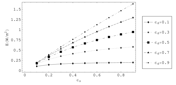
Figure 4: The amount of heat transfer by radiation in the system of two infinite planes in vacuum

III Radiative heat transfer in the case of semi-transmissive walls

If a part $T$ of the incident thermal radiation $I$ passes through the wall (supposed thermic ”thin”) and another part $R$ is returned to the region where it came, it may be possible that, in certain condition, the total net heat flux to be diminished.

In steady state conditions we may write

$$I=T+R+A$$ (21)

where $A$ is the radiation amount that is absorbed by the wall.

If we denote by

$$t=\frac{T}{I},\;r=\frac{r}{I},\;e=\frac{A}{I}$$ (22)

the transmissivity, reflexivity and emissivity of the wall, taking into account the Kirchhoff low of radiation which states that the emitted radiation is equal with the absorbed one, we obtain

$$t=1-e-t$$ (23)

Therefore the equations (8) and (9) have to be written with this reflection coefficient instead $1-e$, so that the net flux emitted by the semi-transparent wall $S_{a}$ and absorbed by $S_{b}$ is

$${E_{st}}={e_{2}}{e_{1}}\sigma\frac{T_{a}^{4}-T_{b}^{4}}{{1-(1-{e_{1}}-t_{1})(1-{e_{2}}-t_{2})}}$$ (24)

If we use a wall with a transparency close to

$$t=1-e$$ (25)

(an ideal case of semi-transparency) then the denominator in the relationship (11) becomes unity, and the thermal flux emitted by this wall and absorbed by the other becomes

$${E_{ab}}={e_{2}}{e_{1}}\sigma\left(T_{a}^{4}-T_{a}^{4}\right)$$ (26)

which reduces the heat transfer by the ratio

$$\frac{E}{E_{st}}=\frac{1}{{1-(1-{e_{1}})(1-{e_{2}})}}$$ (27)

For example, with a typical high reflective surface with $e=0.1$, if the transmissivity is $t=0.9$, the heat transfer reduction ratio is almost five.

However, for heat isolation purposes one may take into account the necessity that the transmitted part of the flux may still be absorbed after the final, coldest wall. That is why the walls must have an unidirectional transparency, from the colder wall to the warmer one. This way, the thermal radiation is reflected to the exterior of the system and dissipated there.

Hence, the right formula for calculating the heat transfer by radiation is obtained considering $t_{2}=0$ in the expression (24)

$${E_{st}}={e_{2}}{e_{1}}\sigma T_{a}^{4}\frac{1}{{1-(1-{e_{1}}-t_{1})(1-{e_{2}})}}$$ (28)

In the ideal case given by the condition (25), the net thermal flux is given by equation (26), being considerably lower than in the opaque wall case.

If there are $n$ walls with the same emissivity $e$ and one side transparency $t=1-e$, the net thermal flux is obtained with an expression similar to (29)

$$E_{st}=\frac{e}{n-1}\sigma(T_{1}^{4}-T_{n}^{4})$$ (29)

IV Numerical results and conclusions

The numerical results obtained for a system of two walls with ideal transparency (the warmer one) are presented in table 2 and figure 5. One may notice an important reduction of the radiation flux especially for the common case of low emissivity values.

Table 2: The heat transfer power reported to the surface between two plane ideally semi-transparent walls, for various values of the emissivity of the right side and the left side ($\rm W/m^{2}$).

${}_{e_{l}}\backslash^{e_{r}}$	0.1	0.2	0.3	0.4	0.5	0.6	0.7	0.8	0.9
0.1	0.02	0.04	0.06	0.08	0.1	0.12	0.14	0.159	0.179
0.2	0.04	0.08	0.12	0.159	0.199	0.239	0.279	0.319	0.359
0.3	0.06	0.12	0.179	0.239	0.299	0.359	0.419	0.478	0.538
0.4	0.08	0.159	0.239	0.319	0.399	0.478	0.558	0.638	0.717
0.5	0.1	0.199	0.299	0.399	0.498	0.598	0.698	0.797	0.897
0.6	0.12	0.239	0.359	0.478	0.598	0.717	0.837	0.957	1.076
0.7	0.14	0.279	0.419	0.558	0.698	0.837	0.977	1.116	1.256
0.8	0.159	0.319	0.478	0.638	0.797	0.957	1.116	1.275	1.435
0.9	0.179	0.359	0.538	0.717	0.897	1.076	1.256	1.435	1.614

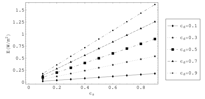
Figure 5: The amount of heat transfer by radiation in the system of two infinite planes in vacuum

Of course, there are technological difficulties concerning the obtaining of the right condition of transparency, but it may be achieved using thin film deposition of materials with the proper index of refraction. One may use the Fresnel formulae for the reflective coefficient calculus, but it has to be considered the temperature and especially the wavelength dependence of the index of refraction of the involved materials, and some other special effects mentioned in the literature Robi .

The presented formulae may be used as a first step in evaluating the performances of cryogenic shields, but surely some experimental steps have to be included for a final cryostat design.

REFERENCES

REFERENCES

- (1) S. Spanulescu,arXiv:0902.4144v1 (2009)
- (2) R.Siegel, J. R. Howell, Thermal Radiation Heat Transfer, Hemisphere, Washington DC, 1992.
- (3) A. Schirrmacher, HSPS, 33, 2, 299-335 (2003)
- (4) http://www.monarchserver.com/TableofEmissivity.pdf
- (5) L. D. Landau and E.M. Lifshitz, Statistical Physics, Elsevier, Amsterdam (2005).
- (6) M. Marinescu, A. Chisacof, P. Raducanu, A. O. Motorcea, Bazele Termodinamicii tehnice, vol. 2, Politehnica Press, Bucharest, 2009
- (7) P-M. L. Robitaille. An analysis of universality in blackbody radiation. Progress in Physics, 2, 22 23,(2006)