Bipolar Molecular Outflows and Hot Cores in GLIMPSE Extended Green Objects (EGOs)

Abstract

We present high angular resolution Submillimeter Array (SMA) and Combined Array for Research in Millimeter-wave Astronomy (CARMA) observations of two GLIMPSE Extended Green Objects (EGOs)–massive young stellar object (MYSO) outflow candidates identified based on their extended 4.5 $\mu$m emission in Spitzer images. The mm observations reveal bipolar molecular outflows, traced by high-velocity ¹²CO(2-1) and HCO⁺(1-0) emission, coincident with the 4.5 $\mu$m lobes in both sources. SiO(2-1) emission confirms that the extended 4.5 $\mu$m emission traces active outflows. A single dominant outflow is identified in each EGO, with tentative evidence for multiple flows in one source (G11.92$-$0.61). The outflow driving sources are compact millimeter continuum cores, which exhibit hot-core spectral line emission and are associated with 6.7 GHz Class II CH₃OH masers. G11.92$-$0.61 is associated with at least three compact cores: the outflow driving source, and two cores that are largely devoid of line emission. In contrast, G19.01$-$0.03 appears as a single MYSO. The difference in multiplicity, the comparative weakness of its hot core emission, and the dominance of its extended envelope of molecular gas all suggest that G19.01$-$0.03 may be in an earlier evolutionary stage than G11.92$-$0.61. Modeling of the G19.01$-$0.03 spectral energy distribution suggests that a central (proto)star (M $\sim$10 M_⊙) has formed in the compact mm core (M_gas $\sim$12-16M_⊙), and that accretion is ongoing at a rate of $\sim$10^-3 M_⊙ year^-1. Our observations confirm that these EGOs are young MYSOs driving massive bipolar molecular outflows, and demonstrate that considerable chemical and evolutionary diversity are present within the EGO sample.

1 Introduction

Massive star formation remains a poorly understood phenomenon, largely due to the difficulty of identifying and studying massive young stellar objects (MYSOs) in the crucial early active accretion and outflow phase. During the earliest stages of their evolution, young MYSOs remain deeply embedded in their natal clouds. Most massive star-forming regions are also distant ($>$ 1kpc) and crowded, with massive stars forming in close proximity to other MYSOs and to large numbers of lower-mass YSOs. Studying the early stages of massive star formation thus requires high angular resolution observations (to resolve individual objects in crowded regions) at long wavelengths unaffected by extinction.

Large-scale Spitzer surveys of the Galactic Plane have yielded a promising new sample of young MYSOs with active outflows, which may be inferred to be actively accreting. Identified based on their extended 4.5 $\mu$m emission in Spitzer images, these sources are known as “Extended Green Objects (EGOs)” (Cyganowski et al., 2008, 2009) or “green fuzzies” (Chambers et al., 2009) from the common coding of the 4.5 $\mu$m band as green in 3-color IRAC images. In active protostellar outflows, the Spitzer 4.5 $\mu$m broadband flux can be dominated by emission from shock-excited molecular lines (predominantly H₂: Smith & Rosen, 2005; Smith et al., 2006; Davis et al., 2007; Ybarra & Lada, 2009; Ybarra et al., 2010; De Buizer & Vacca, 2010). The resolution of Spitzer at 4.5 $\mu$m ($\sim$2^′′) is sufficient to resolve the extended emission from outflows in massive star forming regions nearer than $\sim$7 kpc. Over 300 EGOs have been cataloged in the Galactic Legacy Infrared Mid-Plane Survey Extraordinaire (GLIMPSE-I) survey area by Cyganowski et al. (2008). The mid-infrared (MIR) colors of EGOs are consistent with those of young protostars still embedded in infalling envelopes (Cyganowski et al., 2008). A majority of EGOs are also associated with infrared dark clouds (IRDCs), identified by recent studies as sites of the earliest stages of massive star and cluster formation (e.g. Rathborne et al., 2007; Chambers et al., 2009).

Remarkably high detection rates for two diagnostic types of CH₃OH masers in high-resolution Very Large Array (VLA) surveys provide strong evidence that GLIMPSE EGOs are indeed massive YSOs with active outflows (Cyganowski et al., 2009). There are two Classes of CH₃OH masers, both associated with star formation, but excited under different conditions by different mechanisms. Class II 6.7 GHz CH₃OH masers are radiatively pumped by IR emission from warm dust (e.g. Cragg et al., 2005, and references therein) and are associated exclusively with massive YSOs (e.g. Minier et al., 2003; Bourke et al., 2005; Xu et al., 2008; Pandian et al., 2008). Class I 44 GHz CH₃OH masers are collisionally excited in molecular outflows, and particularly at interfaces between outflows and the surrounding ambient cloud (e.g. Plambeck & Menten, 1990; Kurtz et al., 2004). Of a sample of 28 EGOs, $>$64% have 6.7 GHz Class II CH₃OH masers (nearly double the detection rate of surveys using other MYSO selection criteria), and of these 6.7 GHz maser sources, $\sim$89% also have 44 GHz masers (Cyganowski et al., 2009).

A complementary James Clerk Maxwell Telescope (JCMT; resolution $\sim$20^′′) molecular line survey towards EGOs with 6.7 GHz CH₃OH maser detections found SiO(5-4) emission and HCO⁺(3-2) line profiles consistent with the presence of active molecular outflows (Cyganowski et al., 2009). SiO is particularly well-suited to tracing active outflows, as it persists in the gas phase for only $\sim$10⁴ years after being released by shocks (e.g. Pineau des Forets et al., 1997). A single-dish (resolution $\sim$80^′′) 3 mm spectral line survey of all EGOs visible from the northern hemisphere by Chen et al. (2010) found associated gas/dust clumps of mass 69-29000 M_⊙, consistent with the identification of EGOs as MYSOs. The nature of the driving sources of the 4.5 $\mu$m outflows is only loosely constrained by the survey results. Bright ultracompact (UC) HII regions are, in most cases, ruled out as powering sources by the lack of VLA 44 GHz continuum detections (Cyganowski et al., 2009). A high detection rate (83%) for thermal CH₃OH emission in the Cyganowski et al. (2009) JCMT survey indicates the presence of warm dense gas, and possible hot core line emission.

Further understanding of the nature of EGOs, and their implications for the mode(s) of high-mass star formation, requires identifying the driving source(s) and characterizing their physical properties, as well as those of the outflows associated with EGOs. Interferometric millimeter-wavelength line and continuum observations provide access to direct tracers of molecular outflows and dense, compact gas and dust cores, including a wealth of chemical diagnostics. In this paper, we present Submillimeter Array (SMA) and Combined Array for Research in Millimeter-wave Astronomy (CARMA) observations at 1 and 3 mm of two EGOs from the Cyganowski et al. (2009) sample: G11.92$-$0.61 and G19.01$-$0.03. The targets were chosen to have bipolar (and in some cases quadrupolar) 4.5 $\mu$m morphology, associated 24 $\mu$m emission, associated (sub)mm continuum emission in single-dish surveys, and 6.7 Class II and 44 GHz Class I CH₃OH maser detections in the Cyganowski et al. (2009) survey. The promise of extended 4.5 $\mu$m emission as a MYSO diagnostic lies largely in its ability to identify very young sources with ongoing accretion and outflow that are missed by other sample selection methods. These sources had not been targeted for study prior to their identification as EGOs and inclusion in the Cyganowski et al. (2009) sample, and very little is known about them beyond the results of that survey (see also §3.1.1 and §3.2.1). In §2 we describe our observations, and in §3 we present our results. In §4 we discuss the physical properties of the compact cores and outflows associated with our target EGOs, and in §5 we summarize our conclusions.

2 Observations

2.1 Submillimeter Array (SMA)

SMA observations of our target EGOs were obtained on 23 June 2008 with eight antennas in the compact-north configuration. The observational parameters, including calibrators, are summarized in Table 1. Two pointings were observed in a single track: G11.92$-$0.61 at $\alpha=$18^h13^m58^s.1, $\delta=-$18^∘54′16$\farcs$7, and G19.01$-$0.03 at $\alpha$=18^h25^m44^s.8, $\delta=-$12^∘22′45$\farcs$8 (J2000). The average 225 GHz opacity during the observations was $\sim$0.26, with typical system temperatures at source transit of 220 K. In the compact-north configuration, the array is insensitive to smooth structures larger than $\sim$20^′′. The projected baseline lengths ranged from 7 to 88 k$\lambda$. The double-sideband SIS receivers were tuned to a local oscillator frequency of 225.11 GHz, providing coverage of 219.1-221.1 GHz in the lower sideband (LSB) and 229.1-231.1 GHz in the upper sideband (USB). The spectral lines detected are reported in §3.1.3 and §3.2.3.

Initial calibration of the data was performed in MIRIAD. Each sideband was reduced independently, and the calibrated data were exported to AIPS. The AIPS task UVLSF was used to separate the line and continuum emission, using only line-free channels to estimate the continuum. The continuum data were then self-calibrated, and the solutions transferred to the line data. After self-calibration, the continuum data from the lower and upper sidebands were combined. Imaging was performed in CASA using Briggs weighting and a robust parameter of 0.5. The synthesized beam size is 3$\farcs$2$\times$1$\farcs$8 (P.A.$=$59^∘) for G11.92 and 3$\farcs$2$\times$1$\farcs$7 (P.A.$=$63^∘) for G19.01. The 1$\sigma$ rms noise level in the continuum images is 3.5 mJy beam^-1. The correlator was configured to provide a uniform spectral resolution of 0.8125 MHz. The line data were resampled to a velocity resolution of 1.1 km s^-1, then Hanning smoothed. The typical noise level in a single channel of the Hanning-smoothed spectral line images is 100 mJy beam^-1. The ¹²CO data were further smoothed to a resolution of 3.3 km s^-1; the noise in a single channel is 60 mJy beam^-1. All measurements were made from images corrected for the primary beam response.

Flux calibration was based on observations of Uranus and a model of its brightness distribution using the MIRIAD task smaflux. Comparison of the derived fluxes of the observed quasars (including 3C279, included as an alternate bandpass calibrator) with SMA flux monitoring suggests that the absolute flux calibration is good to $\lesssim$15%. The absolute position uncertainty is estimated to be 0$\farcs$3.

2.2 Combined Array for Research in Millimeter-wave Astronomy (CARMA)

Our 3 mm CARMA observations were obtained on 29 July 2008 (G11.92$-$0.61) and 30 July 2008 (G19.01$-$0.03) in the D-configuration with 15 antennas (six 10.4 m and nine 6.1 m antennas). The observational parameters, including calibrators, are summarized in Table 1. The projected baselines ranged from 1.5 to 31 k$\lambda$ for the 29 July observations and from 1.5 to 36.5 k$\lambda$ for the 30 July observations. The correlator was configured to cover SO (2₂-1₁) at 86.094 GHz (E_upper=19.3 K) in LSB, SiO (2-1) at 86.846 GHz (E_upper=6.3 K) in LSB and HCO⁺(1-0) at 89.189 GHz (E_upper=4.3 K) in USB with 31 MHz windows. Each 31 MHz window consisted of 63 channels, providing a spectral resolution of 0.488 MHz ($\sim$1.7 km s^-1) and velocity coverage of $\sim$100 km s^-1. In addition, the correlator setup included two 500 MHz (pseudo)continuum bands, each comprised of 15 channels: one in LSB centered at $\sim$85.7 GHz and one in USB centered at $\sim$90.3 GHz. In the D-configuration, the array is insensitive to smooth structures larger than $\sim$50^′′. During the observations, the 230 GHz opacity ranged from $\sim$0.47 to 0.5 on 29 July and from $\sim$0.46-0.54 on 30 July. Typical (SSB) system temperatures at source transit were $\sim$230-280 K on 29 July and $\sim$190-240 K on 30 July. The phase center was $\alpha=$18^h13^m58^s.1, $\delta=-$18^∘54′16$\farcs$7 (J2000) on 29 July (G11.92$-$0.61), and $\alpha=$18^h25^m44^s.8, $\delta=-$12^∘22′45$\farcs$8 (J2000) on 30 July (G19.01$-$0.03).

The data were calibrated in MIRIAD and imaged in CASA, using Briggs weighting and a robust parameter of 0.5. The synthesized beamsize is 6$\farcs$8$\times$5$\farcs$1 (P.A.$=$11^∘) for G11.92 and 5$\farcs$7$\times$5$\farcs$1 (P.A.$=$-27^∘) for G19.01. Each band was reduced independently. The 3 mm continuum data for G11.92$-$0.61 are not presented here because of aliasing from IRAS 18110-1854, which is a much brighter continuum source than the target EGO. The IRAS source is $\sim$1′ northeast of the EGO, within the primary beam FWHP of the 6.1 m antennas ($\sim$130^′′) but only at the 20% response level of the primary beam of the 10.4 m antennas (FWHP $\sim$80^′′). For G19.01$-$0.03, the continuum data from the upper and lower sidebands were combined to make a final continuum image with a 1$\sigma$ rms noise level of 0.5 mJy beam^-1. All line data were Hanning smoothed to improve the signal to noise. The noise level in a single channel of the Hanning-smoothed spectral line images is $\sim$12 mJy beam^-1 for G11.92$-$0.61 and $\sim$9 mJy beam^-1 for G19.01$-$0.03. No continuum subtraction was performed, as the continuum contribution to each channel of the line data is negligible. For G19.01$-$0.03, the 3.4 mm continuum peak intensity (9.4 mJy beam^-1) is less than the 1$\sigma$ rms level in the line datacube (10 mJy beam^-1). For G11.92$-$0.61, extrapolating the 1.3 mm continuum peak intensity to 3.4 mm (assuming a spectral index of three) likewise predicts a continuum contribution to the line data at the $\lesssim$1$\sigma$ level. All measurements were made from images corrected for the convolved primary beam response of the heterogeneous CARMA array; in CASA this calculation is done in the visibility domain.

Flux calibration was based on observations of Uranus and a model of its brightness distribution using the MIRIAD task smaflux. Comparison of the derived fluxes of the observed quasars (including 3C273, observed as an alternate bandpass calibrator) with CARMA flux monitoring suggests that the absolute flux calibration is good to $\lesssim$15%.

In addition to the 3 mm observations described above, we obtained 1 mm observations of G11.92$-$0.61 with CARMA in the C-configuration on 25 April 2008 with eleven antennas (three 10.4 m antennas and eight 6.1 m antennas). The projected baselines ranged from 9 to 184.5 k$\lambda$, and the phase center was $\alpha=$18^h13^m58^s.1 $\delta=-$18^∘54′16$\farcs$7 (J2000). In the C-configuration, the array is insensitive to smooth structures larger than $\sim$15^′′. The (SSB) system temperature ranged from $\sim$400-600 K during the observations. The correlator was configured to cover SiO(5-4) at 217.105 GHz and DCN(3-2) at 217.239 GHz in LSB and SO(5₆-4₅) at 219.949 GHz and CH₃OH(8_0,8-7_1,6) at 220.078 GHz in USB with 62 MHz windows and two 500 MHz (pseudo)continuum windows centered at $\sim$216.45 GHz (LSB) and 220.75 GHz (USB). Due to the high system temperatures and limited integration time, only the 500 MHz bands have sufficient signal-to-noise. The USB 500 MHz window encompassed the CH₃CN(J=12-11) ladder, thus only the LSB ($\sim$216.5 GHz) (psuedo)continuum data are presented here. The absolute flux scale was set assuming a flux of 2.69 Jy for J1733-130 based on quasar flux monitoring. The uncertainty in the absolute amplitude calibration is estimated to be $\sim$20%. The data were calibrated in MIRIAD and imaged in CASA, using Briggs weighting and a robust parameter of 0.5. The resulting 1 mm continuum image has a synthesized beamsize of 1$\farcs$44$\times$0$\farcs$87 (P.A.$=$25^∘) and a 1$\sigma$ rms noise level of 4.3 mJy beam^-1. As with the 3 mm data, all measurements were made from images corrected for the response of the heterogeneous primary beams.

3 Results

3.1 G11.92$-$0.61

3.1.1 Previous Observations: G11.92$-$0.61

The EGO G11.92$-$0.61 is $\sim$1′ SE of the more evolved massive star forming region IRAS 18110-1854. Single dish (sub)mm continuum maps targeting the IRAS source show a millimeter/submillimeter clump coincident with the EGO (Walsh et al., 2003; Faúndez et al., 2004; Thompson et al., 2006). Strong ($>$240 Jy) H₂O maser emission associated with the EGO was likewise serendipitously detected in VLA observations targeting the IRAS source (Hofner & Churchwell, 1996). The H₂O maser source was subsequently included in the large single-dish ¹²CO survey of Shepherd & Churchwell (1996), who detected broad ¹²CO line wings.

The MIR emission of G11.92$-$0.61 is characterized by a bipolar 4.5 $\mu$m morphology, with a NE and a SW lobe. The EGO is located in an IRDC (Cyganowski et al., 2008, see also Fig. 1a). The SW lobe is coincident with strong, blueshifted 44 GHz Class I CH₃OH masers, while the NE lobe is surrounded by an arc of systemic to slightly redshifted 44 GHz masers (Cyganowski et al., 2009). Elongated 24 $\mu$m emission is coincident with the NE 4.5 $\mu$m lobe, as are two 6.7 GHz Class II CH₃OH masers (Fig. 1). This EGO is unique among the Cyganowski et al. (2009) sample in having multiple spatially and kinematically distinct loci of 6.7 GHz Class II CH₃OH maser emission. The extended 24 $\mu$m morphology and multiple 6.7 GHz maser spots suggest the possible presence of multiple MYSOs. SiO(5-4) and thermal CH₃OH(5_2,3-4_1,3) emission were detected towards G11.92$-$0.61 in single-pointing JCMT observations (resolution $\sim$20^′′) targeted at the NE lobe/24 $\mu$m source (Cyganowski et al., 2009). No 44 GHz continuum emission was detected towards the EGO to a 5$\sigma$ sensitivity limit of 7 mJy beam^-1 (resolution 0$\farcs$99 $\times$ 0$\farcs$44, Cyganowski et al., 2009). We adopt the near kinematic distance from Cyganowski et al. (2009) for G11.92$-$0.61: 3.8 kpc.

3.1.2 Continuum Emission: G11.92$-$0.61

Our 1.3 mm SMA and 1.4 mm CARMA data resolve three distinct compact continuum sources (Fig. 1a,b). These sources are designated MM1, MM2, and MM3 in order of descending peak intensity. Table 2 lists the observed properties of each source, including the integrated flux density and deconvolved source size determined from a single two-dimensional Gaussian fit. The (sub)mm clump coincident with the EGO is visible in the 1.2 mm SEST/SIMBA map (resolution 24^′′) of Faúndez et al. (2004). No parameters are tabulated, however, so we cannot compute the fraction of the single-dish flux recovered by the interferometers.

All three mm continuum sources are coincident with the NE 4.5 $\mu$m lobe. As shown in Figure 1b, the MIPS 24 $\mu$m emission associated with the EGO is elongated along a N-S axis, and encompasses both MM1 and MM3. The MIPS 24 $\mu$m image is saturated, introducing considerable ($\sim$2-4^′′) uncertainty into the determination of the 24 $\mu$m centroid position (see also Cyganowski et al., 2009). Figure 1b shows, however, that the (saturated) 24$\mu$m peak lies $\sim$1-2^′′ N of MM1, and roughly between MM1 and MM3. The MIPS 24 $\mu$m counterpart thus likely consists of blended emission from these two sources. MM1 and MM3 are also coincident with 6.7 GHz Class II CH₃OH masers reported by Cyganowski et al. (2009) (Fig. 1a,b). The CARMA 1.4 mm centroid position of MM1 is offset $\sim$0$\farcs$6 ($\gtrsim$ 2100 AU) to the north of the intensity-weighted position of the southern 6.7 GHz CH₃OH maser group (G11.918-0.613), and the CARMA 1.4 mm centroid position for MM3 is offset $\sim$0$\farcs$4 ($\gtrsim$ 1500 AU) to the northeast of the intensity-weighted position of the northern 6.7 GHz CH₃OH maser group (G11.919$-$0.613). The H₂O maser reported by Hofner & Churchwell (1996) is also coincident with MM1 to within the astrometric uncertainties (Fig. 1b). Notably, MM2 is offset to the northwest by $\gtrsim$4^′′ ($\gtrsim$ 14800 AU) from the 24 $\mu$m peak, and is not associated with a 6.7 GHz CH₃OH maser.

3.1.3 Compact Molecular Line Emission: G11.92$-$0.61

The continuum source MM1 is associated with the richest molecular line emission in the G11.92$-$0.61 complex. Emission in 27 lines of 11 species is detected towards G11.92$-$0.61-MM1 in our SMA observations. Table 3 lists the specific transitions, frequencies, and upper-state energies of lines detected at $\geq$3$\sigma$. Figure 2 shows the spectrum at the MM1 continuum peak across the 4 GHz bandwidth observed with the SMA, with the transitions listed in Table 3 labeled. Table 3 also lists the peak line intensities, line centroid velocities, $\Delta$v_FWHM, and integrated line intensities obtained from single Gaussian fits to lines detected at $>$3$\sigma$ at the MM1 continuum peak. Some line profiles may be affected by outflowing gas; transitions with non-Gaussian shapes are noted in Table 3. ¹²CO and ¹³CO were not fit, as the line profiles are complex and strongly self-absorbed.

The spectrum of G11.92$-$0.61-MM1 is similar to those of hot cores observed with comparable setups with the SMA, such as AFGL 5142 MM2 (Zhang et al., 2007). The EGO spectrum is also similar to that of HH80-81 MM1, the driving source of the HH80-81 radio jet (Qiu & Zhang, 2009), with the notable exception that SO₂(11_5,7-12_4,8) emission (229.347 GHz, E_upper=122 K) is not detected towards G11.91$-$0.61-MM1. Emission from complex oxygen-rich organic molecules characteristic of strong hot cores (such as HCOOCH₃) also is not detected towards G11.92$-$0.61.

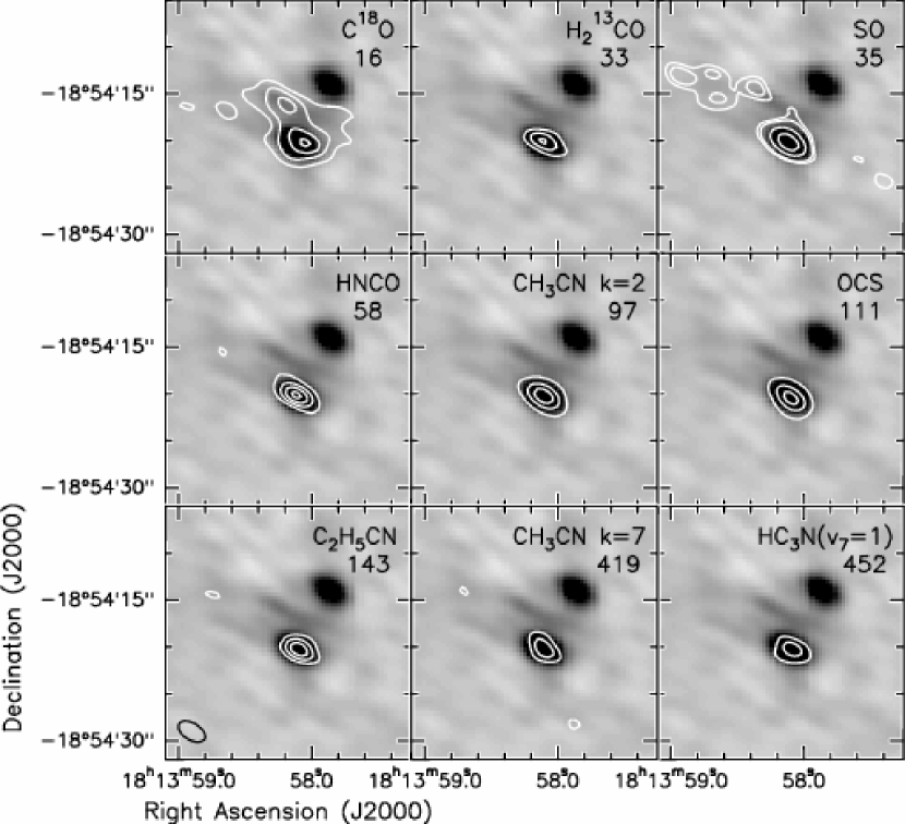
Figure 3: G11.92$-$0.61: The greyscale shows the SMA 1.3 mm continuum emission. Contours are drawn from integrated intensity (moment zero) maps of the indicated molecular line. The species and upper state energy in K of the transition are listed at upper right in each panel. Contour levels are: C¹⁸O: 1.92, 3.84, 5.76, 7.68 Jy beam^-1 km s^-1; H${}_{2}^{13}$CO: 1.65, 3.3, 4.95 Jy beam^-1 km s^-1; SO: 3.3, 4.95, 13.2, 23.1 Jy beam^-1 km s^-1; HNCO: 2.76, 5.52, 8.28, 11.04 Jy beam^-1 km s^-1; CH₃CN (k=2): 2.82, 8.46, 14.1 Jy beam^-1 km s^-1; OCS: 2.4, 7.2, 12 Jy beam^-1 km s^-1; C₂H₅CN: 1.62, 3.24, 4.86 Jy beam^-1 km s^-1; CH₃CN (k=7): 1.8, 3.6 Jy beam^-1 km s^-1; HC₃N(v₇=1): 2.52, 5.04 Jy beam^-1 km s^-1. These contour levels are (3,6,9,12) $\times\sigma$ for C¹⁸O and HNCO; (3,6,9) $\times\sigma$ for H${}_{2}^{13}$CO and C₂H₅CN; (3,9,15) $\times\sigma$ for CH₃CN (k=2) and OCS; (3,6) $\times\sigma$ for CH₃CN (k=7) and HC₃N; and (3,4.5,12,21) $\times\sigma$ for SO. The SMA beam is shown at lower left.

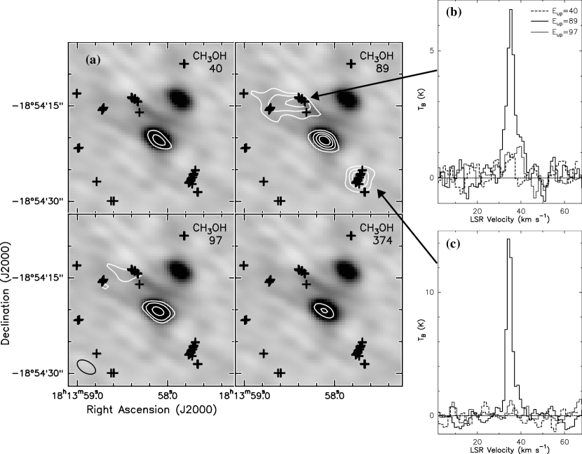
Figure 4: G11.92$-$0.61: (a) The greyscale shows the SMA 1.3 mm continuum emission. Contours are drawn from integrated intensity (moment zero) maps of the indicated CH₃OH line. The upper state energy in K of the transition is given at upper right in each panel. Contour levels are: E_upper=40 K: 2.2, 4.4 Jy beam^-1 km s^-1; E_upper=89K: 2.52, 5.04, 7.56, 10.08 Jy beam^-1 km s^-1; E_upper=97 K: 2,4,8 Jy beam^-1 km s^-1; E_upper=374 K: 2.8, 5.6 Jy beam^-1 km s^-1. These contour levels are (4,8) $\times\sigma$ for the E_upper=40 K and E_upper=374 K transitions, (4,8,12,16) $\times\sigma$ for the E_upper=89 K transition, and (4,8,16) $\times\sigma$ for the E_upper=97 K transition. Black crosses mark the positions of 44 GHz Class I CH₃OH masers from Cyganowski et al. (2009). The SMA beam is shown at lower left. (b) and (c): Spectra at the peak positions of the indicated CH₃OH (8_-1,8-7_0,7) emission. Solid line: 8_-1,8-7_0,7 transition (229.759 GHz, E_upper=89 K); dashed line: 3_-2,2-4_-1,4 (230.027 GHz, E_upper=40 K); dotted line: 8_0,8-7_1,6 (220.078 GHz, E_upper=97 K).

Figures 3 and 4 present integrated intensity (moment zero) maps for selected transitions from Table 3. As shown in Figures 3 and 4, emission from most species is compact and coincident with the continuum source MM1. Emission from high-excitation lines (E_upper$\gtrsim$100 K) is detected exclusively towards MM1. In contrast, the continuum source MM2 is devoid of line emission. The only species that exhibits compact emission coincident with the continuum source MM3 is C¹⁸O (Fig. 3). The CH₃OH integrated intensity maps shown in Figure 4 are discussed further in §3.1.5.

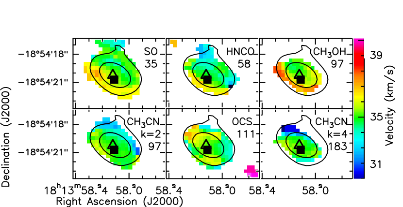
Figure 5: G11.92$-$0.61: First moment maps of the indicated species (colorscale) overlaid with contours of the SMA 1.3 mm continuum emission (levels 10, 30 $\times$ $\sigma=$ 3.5 mJy beam^-1). The inner contour is approximately the size of the SMA beam. E_upper in K is listed under the molecule name in the upper right of each panel. The open triangle marks the water maser position from Hofner & Churchwell (1996). The filled square marks the position of the 6.7 GHz Class II CH₃OH maser from Cyganowski et al. (2009).

Most of the lines detected towards MM1 are quite broad, with $\Delta$v_FWHM of 8-10 km s^-1. The compact molecular line emission exhibits a velocity gradient, from SE (redshifted) to NW (blueshifted) (Fig. 5). As shown in Figure 5, this gradient is consistent across species including SO, HNCO, CH₃OH, and CH₃CN. One possible explanation for this velocity gradient is an unresolved disk, oriented roughly perpendicular to the outflow axis. Higher angular resolution data are required to investigate this possibility. Not all molecules detected towards the hot core show the same velocity gradient. One exception is OCS, which has redshifted emission to the NE and blueshifted emission to the SW. This is consistent with the kinematics of the dominant outflow (§3.1.4), and suggests that the inner regions of the outflow may be contributing significantly to the observed compact OCS emission.

Determining the $v_{LSR}$’s of the mm continuum sources is complicated by the possibility of confusion from outflowing gas or resolved-out emission from the extended envelope. For MM1, there is sufficient agreement among lines that exhibit compact emission and are detected with high signal-to-noise to estimate $v_{LSR}$(MM1)=35.2$\pm$0.4 km s^-1. This is slightly blueward of the $v_{LSR}$ of 36 km s^-1 estimated from the lower angular resolution H¹³CO⁺ observations of Cyganowski et al. (2009). The systemic velocity of MM1 is also blueshifted relative to both the 6.7 GHz Class II CH₃OH masers coincident with MM1 (v$\sim$37.1-37.6 km s^-1; Cyganowski et al., 2009), and the peak H₂O maser velocity (v=40.7 km s^-1; Hofner & Churchwell, 1996). There is also weaker H₂O maser emission at the 6.7 GHz CH₃OH maser velocity. Table 3 lists a Gaussian fit to the C¹⁸O emission towards the MM3 continuum peak. The emission is narrow ($\Delta$v_FWHM=3.5 km s^-1), and has a line centroid velocity of 34.4 km s^-1. Since no other compact line emission is detected associated with MM3, however, it is difficult to be certain whether this velocity represents the MM3 gas $v_{LSR}$. If so, then the thermal gas emission from MM3 is blueshifted by $\geq$ 4 km s^-1 relative to the coincident 6.7 GHz Class II CH₃OH masers, which have velocities of $\sim$38.6-39.5 km s^-1. Since no emission centered on MM2 is detected, its $v_{LSR}$ cannot be determined.

3.1.4 Extended Molecular Line Emission: G11.92$-$0.61

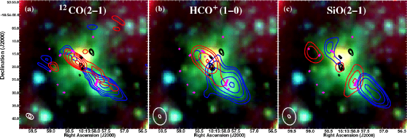
Figure 6: G11.92-0.61: Three color Spitzer images (3.6, 4.5, 8.0 $\mu$m: blue, green, red) overlaid with contours of 1.4 mm continuum emission (black) and high velocity (a) ¹²CO(2-1), (b) HCO⁺(1-0), and (c) SiO(2-1) emission. In each panel, positions of 6.7 GHz CH₃OH masers are marked with black diamonds, and positions of 44 GHz CH₃OH masers are marked with magneta crosses (Cyganowski et al., 2009). Continuum contour levels are 4,5,10,20 $\times$ $\sigma=$ 4.3 mJy beam^-1. The $v_{LSR}$ is $\sim$35 km s^-1 (§3.1.3,4.2). (a) ¹²CO(2-1) emission integrated over v=$-$24.4 to 21.8 km s^-1 (blue) and v=48.1 to 71.2 km s^-1 (red), e.g. $\sim$$v_{LSR}$$\pm$13 km s^-1. Levels are 5,9,17,29,45 Jy beam^-1 km s^-1 for both red and blue contours. The SMA and CARMA beams are shown at lower left. (b) HCO⁺(1-0) emission integrated over v=-14.3 to 21.8 km s^-1 (blue) and 48.1 to 71.1 km s^-1 (red), e.g. $\sim$$v_{LSR}$$\pm$13 km s^-1. Contour levels: Blue: 1.3, 1.8, 2.8, 4.3, 5.8 Jy beam^-1 km s^-1; Red: 1.3, 1.8, 2.8, 3.8 Jy beam^-1 km s^-1. The CARMA beams are shown at lower left. (c) SiO(2-1) emission integrated over v=8.0 to 24.9 km s^-1 (blue) and v=45.1 to 53.5 km s^-1 (red), e.g. $\sim$$v_{LSR}$$\pm$10 km s^-1. Contour levels: Blue: 0.8, 1.0, 1.4, 2.0 Jy beam^-1 km s^-1; Red: 0.6, 0.8, 1.0 Jy beam^-1 km s^-1. The CARMA beams are shown at lower left.

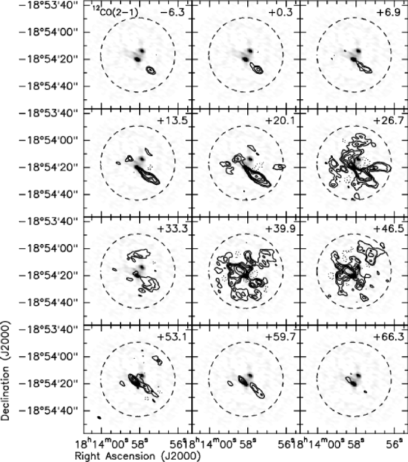
Figure 7: G11.92$-$0.61: Channel maps of ¹²CO(2-1). The greyscale is the 1.3 mm SMA continuum image and the contours are the ¹²CO emission (levels 0.24, 0.48, 0.96, 1.44, 2.16, 3.6 Jy beam^-1(solid), $-$0.24, $-$0.48 Jy beam^-1(dotted)). Each panel is the average of two channels of the smoothed ¹²CO cube; the center velocity of each panel is given at upper right. The contour levels are ($-$8,$-$4,4,8,16,24,36,60) $\times$ the rms in a line-free panel. The field of view shown is the same as in Figures 8 and  9. The dashed circle shows the FWHP of the SMA primary beam. The SMA synthesized beam is shown as a filled ellipse at lower left.

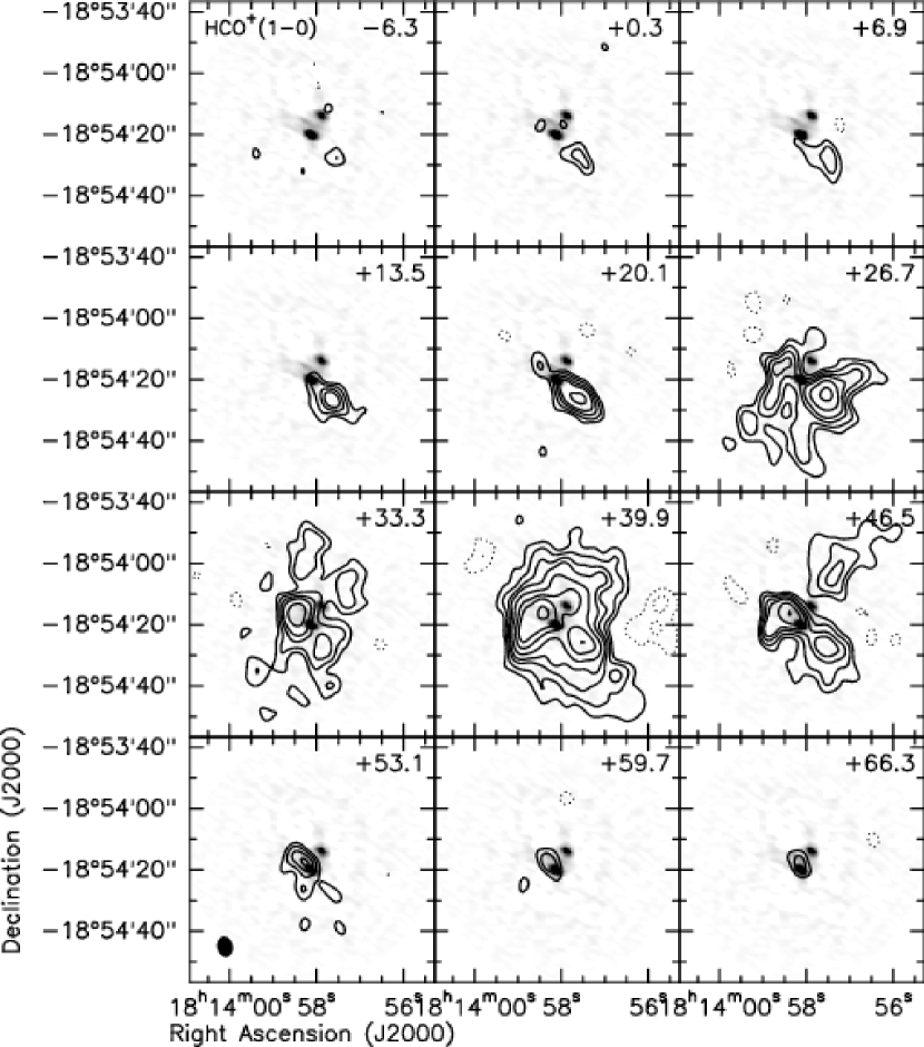
Figure 8: G11.92$-$0.61: Channel maps of HCO⁺(1-0). The greyscale is the 1.3 mm SMA continuum image. The contours are the HCO⁺ emission (levels 0.06, 0.096, 0.144, 0.192, 0.288, 0.432, 0.576, 0.864 Jy beam^-1(solid), $-$0.06, $-$0.096 (dotted)). The contour levels are ($-$8,$-$5,5,8,12,16,24,36,48,72) $\times$ the rms in a line-free panel. The center velocity of each panel is given at upper right. The field of view shown is the FWHP primary beam of the 10 m CARMA antennas (80^′′ square). The CARMA synthesized beam is shown as a filled ellipse at lower left.

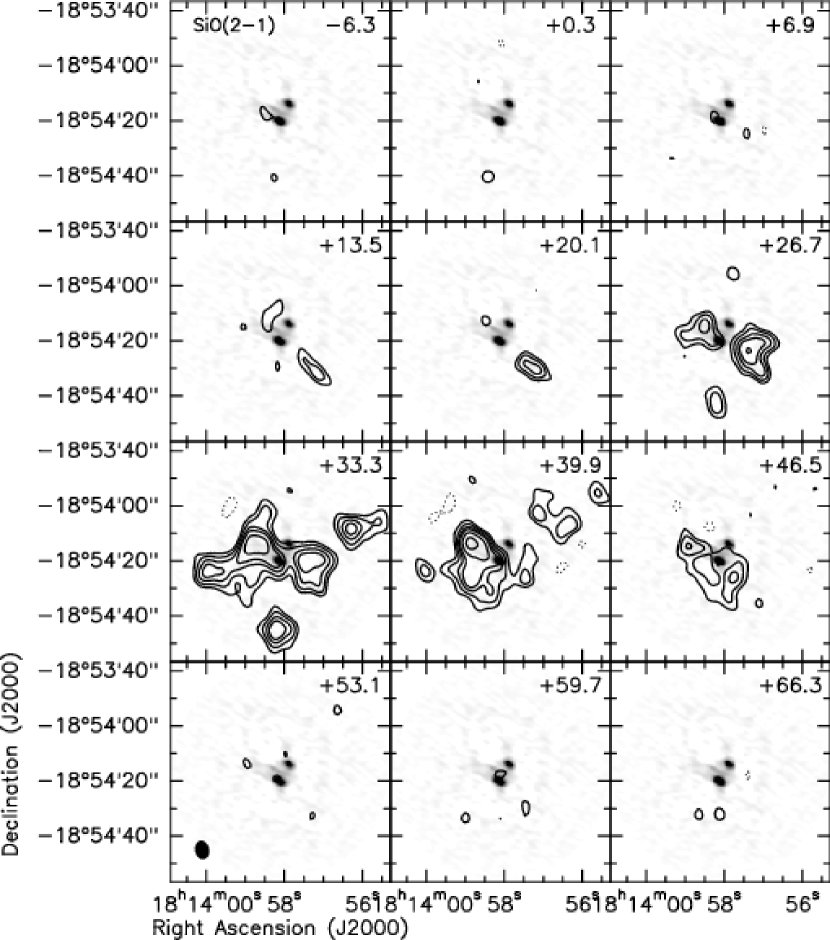
Figure 9: G11.92$-$0.61: Channel maps of SiO(2-1). The greyscale is the 1.3 mm SMA continuum image. The contours are the SiO emission (levels 0.055, 0.088, 0.132, 0.176, 0.264, 0.396 Jy beam^-1(solid), $-$0.055 Jy beam^-1(dotted)). The contour levels are ($-$5,5,8,12,16,24,36) $\times$ the rms in a line-free panel. The center velocity of each panel is given at upper right. The field of view shown is the FWHP primary beam of the 10 m CARMA antennas (80^′′ square). The CARMA synthesized beam is shown as a filled ellipse at lower left.

The observed low-excitation transitions of the abundant molecules ¹²CO and HCO⁺ exhibit extended emission spanning a wide velocity range ($>$ 80 km s^-1) and most of the telescope field of view. Emission in SiO (2-1) is similarly spatially extended, but spans a narrower velocity range ($\sim$40 km s^-1). While the kinematics of this extended emission are complex, the high velocity ($|$v$-$$v_{LSR}$$|\gtrsim$ 13 km s^-1) ¹²CO and HCO⁺ emission are characterized by a bipolar outflow centered on the continuum source MM1 (Fig. 6). To complement the integrated intensity maps of the high velocity gas shown in Figure 6, channel maps of the ¹²CO(2-1), HCO⁺(1-0), and SiO (2-1) emission are shown in Figures 7-9.

The red and blue lobes of the molecular outflow are asymmetric, both spatially and kinematically. The blueshifted lobe, SW of MM1, extends to more extreme velocities ($|$v${}_{max,blue}-$$v_{LSR}$$|$$\sim$59 km s^-1; $|$v${}_{max,red}-$$v_{LSR}$$|$$\sim$36 km s^-1) and further from the continuum source. The blueshifted lobe also exhibits stronger SiO (2-1) emission. The sense of the velocity gradient in the molecular gas agrees with that of 44 GHz Class I CH₃OH masers imaged with the VLA (resolution 0$\farcs$99$\times$0$\farcs$44, Cyganowski et al., 2009). The concentration of blueshifted Class I masers coincides with the blueshifted molecular outflow lobe seen in ¹²CO and HCO⁺ and with the SW 4.5 $\mu$m lobe (Fig. 6a,b). The Class I masers in the arc to the NE have near-systemic or slightly redshifted velocities, consistent with the location and more moderate velocity of the redshifted molecular outflow lobe. In particular, the SE section of the maser arc is coincident with moderately redshifted ¹²CO, HCO⁺, and SiO emission (Figs. 7-9, 39.9 and 46.5 km s^-1 panels; this relatively low-velocity gas is not included in the integrated intensity maps shown in Figure 6).

The morphology and kinematics of the SiO(2-1) emission differ from those of the other outflow tracers, and copious SiO (2-1) emission is detected far from the mm continuum sources (Figs. 6,9). The excitation of low-J rotational lines of SiO, such as the 2-1 transition, depends primarily on the density, n${}_{H_{2}}$ (as opposed to the kinetic temperature, T_kin; Nisini et al., 2007; Jimenez-Serra et al., 2010), and extended (parsec-scale), quiescent ($\Delta$v$\sim$0.8 km s^-1) SiO(2-1) emission has recently been observed towards an IRDC (Jimenez-Serra et al., 2010). The comparatively broad linewidths of the SiO(2-1) emission towards G11.92$-$0.61 indicate that the entirety of the observed SiO emission is attributable to outflow-driven shocks, with bright SiO(2-1) knots likely tracing the impact of these shocks on dense regions in the surrounding cloud.

While the NE(red)-SW(blue) gradient dominates the ¹²CO and HCO⁺ velocity fields, there are other features that suggest multiple outflows may be present. In particular, blueshifted ¹²CO, HCO⁺, and SiO emission are detected NE of MM1 at velocities $\gtrsim$ 10 km s^-1, and redshifted emission SW of MM1 at velocities $\lesssim$ 65 km s^-1 (Figs. 6-9). Near the $v_{LSR}$ of $\sim$35 km s^-1, however, low-velocity outflow emission is confused with emission from ambient gas.

Emission from SO(6₅-5₄) also extends NE and SW of MM1 (Fig. 3). The morphology and kinematics are consistent with this SO emission arising in the dominant outflow; in contrast to SiO, the SO emission is stronger towards the redshifted (NE) outflow lobe. The properties of the lower-excitation SO (2₂-1₁) emission (E_upper=19.3 K) observed with CARMA (not shown) are similar to those seen in SO(6₅-5₄) at higher spatial and spectral resolution with the SMA. Faint SO(6₅-5₄) emission is detected coincident with the MM3 continuum source, at a velocity consistent with that of the C¹⁸O (§3.1.3). However, since the bipolar outflow(s) overlap the MM3 position, it is unclear whether this SO emission is associated with MM3.

3.1.5 Millimeter CH₃OH masers: G11.92$-$0.61

As shown in Figure 4, the morphology of the 229.759 GHz CH₃OH(8_-1,8-7_0,7)E (E_upper=89 K) line emission is strikingly different from that of any other observed CH₃OH transition. There is very strong CH₃OH(8_-1,8-7_0,7) emission to the southwest of MM1, coincident with the brightest 44 GHz CH₃OH(7₀-6₁)A⁺ Class I masers detected by Cyganowski et al. (2009) (Fig. 4). Strong 229.759 GHz CH₃OH emission is also observed NE of MM1, also coincident with 44 GHz Class I masers. The 44 GHz (7₀-6₁) and 229.759 GHz (8_-1,8-7_0,7) lines are both Class I CH₃OH maser transitions. Slysh et al. (2002) first reported 229.759 GHz CH₃OH maser emission towards DR21 (OH) and DR21 West based on observations with the IRAM 30 m telescope. Probable maser emission in this transition has been detected with the SMA in HH 80-81, coincident with a 44 GHz CH₃OH maser (Qiu & Zhang, 2009), and in IRAS 05345+3157 (Fontani et al., 2009).

The CH₃OH(8_-1,8-7_0,7) emission observed NE and SW of G11.92$-$0.61-MM1 is spectrally narrow (Fig. 4b-c). In both cases, the velocity of the mm emission agrees well with the velocities of the coincident 44 GHz masers. The extended appearance of the northeastern 229.759 GHz emission is consistent with emission from multiple masers being blended at the lower spatial resolution of the SMA observations ($\sim$3^′′ compared to $\sim$0$\farcs$5 for the 44 GHz VLA data). Like the studies of Slysh et al. (2002) and Qiu & Zhang (2009), the beamsize of our observations is too large to definitively establish the maser nature of the emission based on its brightness temperature. The peak intensity of the SW CH₃OH(8_-1,8-7_0,7) emission is 3.5 Jy beam^-1, corresponding to T_B=14.3 K. For the NE emission, I_peak=1.6 Jy beam^-1 (T_B=6.6 K). Slysh et al. (2002) use the 229.759/230.027 line ratio as a discrimant between thermal and masing 229.759 GHz emission, with ratios $>$ 3 indicative of non-thermal 229.759 GHz CH₃OH emission. The 230.027 GHz line is a Class II transition, so is not expected to be inverted under conditions that excite 229.759 GHz Class I maser emission (Slysh et al., 2002). The 229.759/230.027 ratios for the SW and NE spots in G11.92$-$0.61 are 100 and 7, respectively. For comparison, the ratio at the MM1 1.3 mm continuum peak is 2, consistent with thermal emission from the hot core. The SW and NE 229.759 GHz emission features coincide spatially and spectrally with 44 GHz Class I CH₃OH masers; this agreement, along with the millimeter line ratios and narrow linewidths, strongly supports the interpretation of these emission features as mm CH₃OH maser emission.

3.2 G19.01$-$0.03

3.2.1 Previous Observations: G19.01$-$0.03

This source was entirely unknown prior to being cataloged as an EGO by Cyganowski et al. (2008). The EGO G19.01$-$0.03 has a striking MIR appearance, with bipolar 4.5 $\mu$m emission centered on a point source detected in GLIMPSE and MIPSGAL images. Cyganowski et al. (2009) detected kinematically complex Class II 6.7 GHz CH₃OH maser emission coincident with the “central” source. Copious 44 GHz Class I CH₃OH maser emission is associated with the 4.5 $\mu$m lobes, with blueshifted masers concentrated to the north of the MIR point source and systemic/redshifted masers to the south (Cyganowski et al., 2009). The EGO is located in an IRDC (Cyganowski et al., 2008), and a (sub)mm continuum source coincident with the EGO is detected in blind single-dish surveys of the Galactic Plane at 1.1 mm and 870 $\mu$m (BGPS and ATLASGAL, Rosolowsky et al., 2010; Schuller et al., 2009). SiO(5-4) and thermal CH₃OH(5_2,3-4_1,3) emission were detected towards G19.01$-$0.03 in single-pointing JCMT observations (resolution $\sim$20^′′) targeted at the MIR point source (Cyganowski et al., 2009). No 44 GHz continuum emission was detected towards the EGO to a 5$\sigma$ sensitivity limit of 5 mJy beam^-1 (resolution 0$\farcs$59 $\times$ 0$\farcs$51, Cyganowski et al., 2009). We adopt the near kinematic distance from Cyganowski et al. (2009) for G19.01$-$0.03: 4.2 kpc.

3.2.2 Continuum Emission: G19.01$-$0.03

At the resolution of our SMA 1.3 mm and CARMA 3.4 mm observations, the millimeter continuum emission associated with the EGO G19.01$-$0.03 appears to arise from a single source, called MM1. The SMA 1.3 mm continuum image is shown in Figure 1c. The position of the peak 3.4 mm continuum emission (not shown) coincides with the 1.3 mm continuum peak. In our SMA 1.3 mm continuum image, we recover 7.6${}^{+1.9}_{-1.4}$% of the single-dish flux density of 3.6${}^{+0.7}_{-0.6}$ Jy measured from the 1.1 mm Bolocam Galactic Plane Survey (BGPS, resolution $\sim$30^′′, Rosolowsky et al., 2010).

The fitted position of MM1 from the SMA 1.3 mm continuum image is coincident with the intensity-weighted position of the Class II 6.7 GHz CH₃OH maser (Cyganowski et al., 2009) and with the GLIMPSE point source SSTGLMC G019.0087-00.0293 within the absolute positional uncertainty of the mm data (0$\farcs$3). The MIPS 24 $\mu$m peak is offset to the NW by $\sim$1$\farcs$3 ($\gtrsim$ 5500 AU). This is consistent, however, with MM1 being coincident with the MIPS 24 $\mu$m source within the absolute positional uncertainty of the MIPSGAL survey (median 0$\farcs$85, up to $\sim$3^′′, Carey et al., 2009).

3.2.3 Compact Molecular Line Emission: G19.01$-$0.03

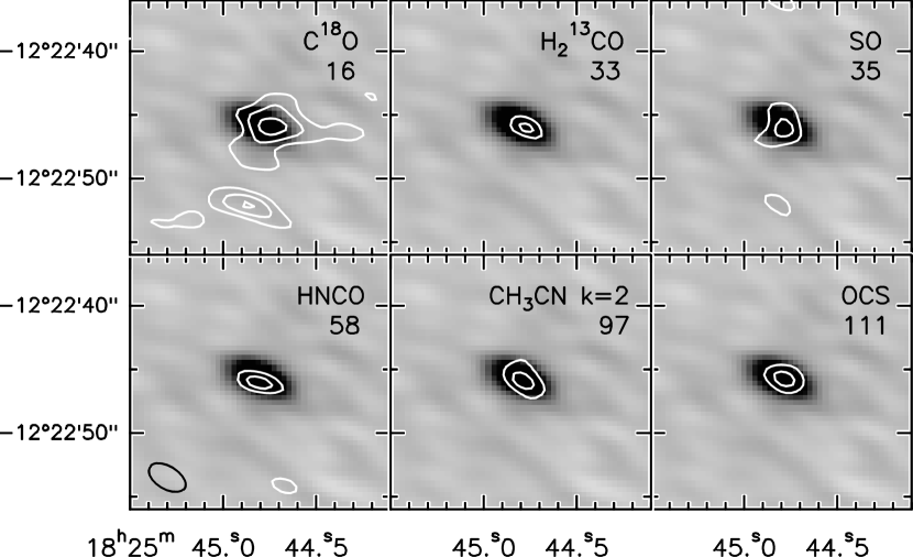
Figure 11: G19.01$-$0.03: The greyscale shows the SMA 1.3 mm continuum emission. Contours are drawn from integrated intensity (moment zero) maps of the indicated molecular line. The species and upper state energy in K of the transition are listed at upper right in each panel. Contour levels are: C¹⁸O: 1.65, 3.3, 4.95 Jy beam^-1 km s^-1; H${}_{2}^{13}$CO: 1.2, 2.0 Jy beam^-1 km s^-1; SO: 0.9, 1.5 Jy beam^-1 km s^-1; HNCO: 1.32, 2.20 Jy beam^-1 km s^-1; CH₃CN (k=2): 1.11, 1.85 Jy beam^-1 km s^-1; OCS: 1.2, 2.4 Jy beam^-1 km s^-1. These contour levels are (3,6,9)$\times$ $\sigma$ for C¹⁸O, (3,5)$\times$ $\sigma$ for H${}_{2}^{13}$CO, SO, HNCO, and CH₃CN, and (3,6)$\times$ $\sigma$ for OCS. The SMA beam is shown at lower left.

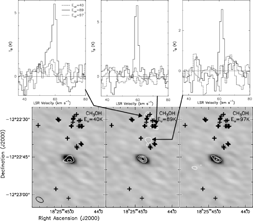
Figure 12: G19.01$-$0.03: The greyscale shows the SMA 1.3 mm continuum emission. Contours are drawn from integrated intensity (moment zero) maps of the indicated CH₃OH line. The upper state energy in K of the transition is given at upper right in each panel. Contour levels are: E_upper=40 K: 1.11, 1.85 Jy beam^-1 km s^-1; E_upper=89 K: 1.02, 1.7, 2.38 Jy beam^-1 km s^-1; E_upper=97 K: 1.32, 2.20, 3.08 Jy beam^-1 km s^-1. These contour levels are (3,5)$\times$ $\sigma$ for the E_upper=40 K transition and (3,5,7)$\times$ $\sigma$ for the E_upper=89 K and E_upper=97 K transitions. Black crosses mark the positions of 44 GHz Class I CH₃OH masers from Cyganowski et al. (2009). The SMA beam is shown at lower left. Spectra are shown at the peak position of the indicated CH₃OH (8_-1,8-7_0,7) emission spot. Solid line: 8_-1,8-7_0,7 transition (229.759 GHz, E_upper=89 K); dashed line: 3_-2,2-4_-1,4 (230.027 GHz, E_upper=40 K); dotted line: 8_0,8-7_1,6 (220.078 GHz, E_upper=97 K).

Emission in 15 lines of 9 species is detected towards G19.01$-$0.03-MM1 in our SMA observations. Table 4 lists the specific transitions, frequencies, and upper-state energies of lines detected at $\geq$3$\sigma$. Figure 10 shows the spectrum at the MM1 continuum peak across the 4 GHz bandwidth observed with the SMA, with the transitions listed in Table 4 labeled. As shown by a comparison of Figures 2 and 10, many of the stronger lines detected towards G11.92$-$0.61-MM1 are also detected towards G19.01$-$0.03-MM1. These lines are much weaker towards G19.01$-$0.03, however, and emission from higher-energy transitions (E_upper$>$ 200 K) is notably lacking. The highest-energy line detected towards G19.01$-$0.03-MM1 is the k=4 component of the CH₃CN(12-11) ladder (E_upper=183 K), and this line is very weak ($\sim$3.5$\sigma$). Other than the k=3 and k=4 CH₃CN lines, no line emission with E_upper$>$100 K is detected towards G19.01$-$0.03-MM1. As shown in Figures 11 and 12, emission from most species is compact and coincident with the continuum source.

Table 4 also lists the peak line intensities, line center velocities, $\Delta$v_FWHM, and integrated line intensities obtained from single Gaussian fits to lines detected at $>$3$\sigma$ at the G19.01$-$0.03 MM1 continuum peak. Some line profiles may be affected by outflowing gas; lines not well fit by a Gaussian are noted in Table 4. As for G11.92$-$0.61, the ¹²CO and ¹³CO lines were not fit, as the line profiles are non-Gaussian and, in the case of ¹²CO, strongly self-absorbed. As Table 4 demonstrates, there is good agreement among the central velocities determined from the different species and transitions. Considering all lines detected at $>$5$\sigma$, $v_{LSR}$(MM1)=59.9$\pm$1.1 km s^-1. This is in good agreement with the central velocities of H¹³CO⁺(3-2) (v_center=59.9$\pm$0.1 km s^-1) and CH₃OH(5_2,3-4_1,3) (v_center=59.7$\pm$0.2 km s^-1) observed with the JCMT (resolution $\sim$20^′′, Cyganowski et al., 2009).

Compared to G11.92$-$0.61-MM1, the lines detected towards G19.01$-$0.03-MM1 are relatively narrow. Most of the transitions detected with $>$5$\sigma$ have $\Delta$v${}_{FWHM}<$ 4 km s^-1. The 6.7 GHz Class II CH₃OH masers associated with G19.01$-$0.03-MM1 span a comparatively wide velocity range of $\sim$7.5 km s^-1, from 53.7-61.1 km s^-1 (Cyganowski et al., 2009). The velocity range of the 6.7 GHz CH₃OH maser emission extends much further to the blue of the $v_{LSR}$ than it does to the red.

Figures 11 and  12 present integrated intensity (moment zero) maps for selected transitions in Table 4. The only species in Figure 11 that exhibits significant emission not coincident with the continuum source is C¹⁸O (2-1). (The properties of the SO (2₂-1₁) (E_upper=19.3 K) emission observed with CARMA (not shown) are similar to those of the SO(6₅-5₄) emission observed at higher spatial and spectral resolution with the SMA.) The C¹⁸O emission coincident with the continuum source has near-systemic velocities, while the two knots of C¹⁸O emission to the south of MM1 are redshifted and likely associated with knots in the outflow.

3.2.4 Extended Molecular Line Emission: G19.01$-$0.03

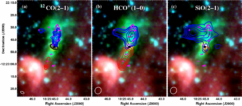
Figure 13: G19.01-0.03: Three color Spitzer images (3.6, 4.5, 8.0 $\mu$m: blue, green, red) overlaid with contours of high velocity (a) ¹²CO(2-1), (b) HCO⁺(1-0), and (c) SiO(2-1) emission. In each panel, positions of 6.7 GHz CH₃OH masers are marked with black diamonds, and positions of 44 GHz CH₃OH masers are marked with magneta crosses (Cyganowski et al., 2009). The $v_{LSR}$ is $\sim$60 km s^-1 (§3.2.3). (a) ¹²CO(2-1) emission integrated over v=$-$46.4 to 19.5 km s^-1 (blue) and v=75.6 to 88.8 km s^-1 (red). Contour levels: Blue: 7.2, 9.6, 12, 15.6, 19.2, 22.8 Jy beam^-1 km s^-1; Red: 4.8, 7.2, 9.6 Jy beam^-1 km s^-1. Black contours: SMA 1.3 mm continuum emission (levels 5,10,30 $\times$ $\sigma=$ 3.5 mJy beam^-1). The SMA beam is shown at lower left. (b) HCO⁺(1-0) emission integrated over v=7.8 to 52.2 km s^-1 (blue) and 68.6 to 83.4 km s^-1 (red), e.g. $\sim$$v_{LSR}$$\pm$8 km s^-1. Contour levels: Blue: 1.0, 1.2, 1.6, 2.2, 3.0, 4.0 Jy beam^-1 km s^-1; Red: 0.6, 0.8, 1.0, 1.2 Jy beam^-1 km s^-1. The CARMA beam is shown at lower left. (c) SiO(2-1) emission integrated over v=26.0 to 52.9 km s^-1 (blue) and v=66.4 to 83.3 km s^-1 (red), e.g. $\sim$$v_{LSR}$$\pm$7 km s^-1. Contour levels: Blue: 0.5, 0.8, 1.2, 1.8, 2.6 Jy beam^-1 km s^-1; Red: 0.5 Jy beam^-1 km s^-1. The CARMA beam is shown at lower left.

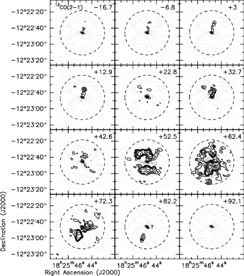
Figure 14: G19.01$-$0.03: Channel maps of ¹²CO(2-1). The greyscale is the 1.3 mm SMA continuum image and the contours are the ¹²CO emission (levels 0.2, 0.4, 0.6, 0.8, 1.2, 1.8, 3 Jy beam^-1(solid), $-$0.2, $-$0.4 Jy beam^-1(dotted)). Each panel is the average of three channels of the smoothed ¹²CO cube; the center velocity of each panel is given at upper right. The contour levels are ($-$8,$-$4,4,8,16,24,36,60) $\times$ the rms in a line-free panel. The field of view shown is the same as in Figures 15 and  16. The dashed circle shows the FWHP of the SMA primary beam. The SMA synthesized beam is shown as a filled ellipse at lower left.

Extended molecular line emission, spanning most of the telescope field of view, is exhibited by ¹²CO(2-1) and HCO⁺(1-0). Extended SiO(2-1) emission is also observed. Figure 13 presents integrated intensity images of high-velocity gas, while Figures 14, 15, and 16 show channel maps of the ¹²CO(2-1), HCO⁺(1-0), and SiO(2-1) emission, respectively.

As shown in Figures 13-15, ¹²CO and HCO⁺ trace a bipolar molecular outflow centered on the continuum source MM1. The outflow axis is roughly N-S, with the blueshifted lobe to the north and the redshifted lobe to the south. This is consistent with the velocity gradient of the 44 GHz Class I CH₃OH masers (Cyganowski et al., 2009). Blueshifted 44 GHz CH₃OH masers are concentrated towards the northern 4.5 $\mu$m lobe, while systemic and redshifted 44 GHz CH₃OH masers are concentrated to the south of the central source. The 44 GHz Class I CH₃OH masers trace the edges of the high-velocity ¹²CO and HCO⁺ lobes remarkably well (Fig. 13a,b). In particular, an arc of 44 GHz masers appears to trace the edges and terminus of the blueshifted ¹²CO jet.

The full velocity range of the ¹²CO outflow is $\sim$135 km s^-1. The kinematics of the outflow are notably asymmetric. The highest-velocity blueshifted gas has $|$v${}_{max,blue}-$$v_{LSR}$$|$$\sim$106 km s^-1, while for the redshifted lobe, $|$v${}_{max,red}-$$v_{LSR}$$|$ is only $\sim$29 km s^-1. The velocity distribution of the 44 GHz CH₃OH masers is also asymmetric with respect to the $v_{LSR}$: $|$v${}_{max,blue,maser}-$$v_{LSR}$$|$$\sim$6.5 km s^-1 while $|$v${}_{max,red,maser}-$$v_{LSR}$$|$$\sim$2.2 km s^-1 (Cyganowski et al., 2009). The blueshifted lobe of the molecular outflow traced by ¹²CO and HCO⁺ is coincident with the northern lobe of extended 4.5 $\mu$m emission. In contrast, the most highly redshifted molecular gas is found south of the brightest 4.5 $\mu$m emission in the southern lobe. The high velocity outflow gas is clumpy. Both the red and blue lobes are characterized by strings of bright knots.

The SiO(2-1) emission differs in kinematics and morphology from the ¹²CO and HCO⁺ emission (Fig. 13). Very little redshifted SiO emission is detected. Blueshifted SiO emission is concentrated north of the continuum source, consistent with the orientation of the ¹²CO/HCO⁺ outflow. The morphology of the blueshifted SiO emission, however, is linearly extended along an E-W axis. Near the systemic velocity ($\sim$60 km s^-1), the SiO emission extends to the south towards the continuum source (Fig. 16). Like the high-velocity ¹²CO and HCO⁺ emission, the SiO emission is characterized by clumps and knots. The strongest blueshifted SiO emission arises from a clump offset to the east of the extended 4.5 $\mu$m emission.

Near the $v_{LSR}$($\sim$60 km s^-1), the ¹²CO image cube shows artifacts from large-scale emission resolved out by the interferometer (Fig. 14). This suggests that near the systemic velocity, the ¹²CO(2-1) emission is dominated by emission from a large-scale extended envelope. This interpretation is consistent with the large spatial extent of the HCO⁺(1-0) emission near the $v_{LSR}$ (Fig. 15).

3.2.5 Millimeter CH₃OH masers: G19.01$-$0.03

As seen in G11.92$-$0.61, the 229.759 GHz CH₃OH(8_-1,8-7_0,7)E (E_upper=89 K) emission towards G19.01$-$0.03 has a very different morphology than any other observed CH₃OH transition. Figure 12 presents integrated intensity maps of the 230.027 GHz (E_upper=40 K), 229.759 GHz, and 220.078 GHz (E_upper=97 K) CH₃OH emission towards G19.01$-$0.03, with the positions of 44 GHz Class I masers from Cyganowski et al. (2009) marked. There are three compact loci of 229.759 GHz CH₃OH emission to the north of MM1, two of which are coincident with numerous 44 GHz masers. Figure 12 also shows the profiles of the 230.027 GHz, 229.759 GHz, and 220.078 GHz CH₃OH emission towards the peak of each of these spots. The 229.759 GHz CH₃OH emission towards these loci is spectrally narrow. Towards the two northern spots, the velocity of the 229.759 GHz CH₃OH emission agrees well with the velocity range of the coincident 44 GHz CH₃OH masers. In the integrated intensity map shown in Figure 12, the southernmost of the three 229.759 GHz CH₃OH emission spots appears to lie between three clusters of 44 GHz CH₃OH masers. The SMA data has much lower spatial and spectral resolution than the 44 GHz VLA data (SMA: 3^′′, 1.6 km s^-1; VLA: 0$\farcs$75, 0.24 km s^-1). Examination of the data cubes shows that the 229.759 GHz CH₃OH emission near this location is consistent with being a blend of masers seen at 44 GHz, given the lower spatial and spectral resolution of the mm data. As shown in Figure 12, the 229.759/230.027 line ratios towards the three spots are all $>$3, consistent with non-thermal 229.759 GHz CH₃OH emission (Slysh et al., 2002, see also §3.1.5). Towards the MM1 continuum peak, this line ratio is 2, consistent with thermal emission.

4 Discussion

4.1 Continuum Sources

4.1.1 Spectral Energy Distributions (SEDs)

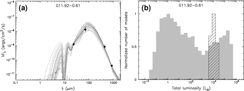
Figure 17: G11.92$-$0.61: (a) Data (black circles) overlaid with the best fit model (solid black line) and other good fits (grey lines) from the Robitaille et al. (2007) model grid. The twenty best fits are shown. (b) Histogram of the bolometric luminosity of the 20 best-fit models (hatched histogram) and all models in the grid (grey histogram).

Unfortunately, the three members of the G11.92$-$0.61 (proto)cluster are not resolved in existing data at wavelengths shorter than 1.3 mm. To better constrain the SED of the protocluster as a whole, we measured the 70 $\mu$m flux density from MIPSGAL images (Carey et al., 2009). We find a flux density of 369 Jy, with an estimated uncertainty of $\sim$50% due to artifacts in the publicly available BCD images (Carey et al., 2009). Walsh et al. (2003) report integrated flux densities of 140 Jy (450 $\mu$m) and 12 Jy (850 $\mu$m) for the (sub)mm clump (G11.92$-$0.64B in their nomenclature). Using these fluxes and the 24 $\mu$m flux from Cyganowski et al. (2009), we fit the 24-850 $\mu$m data using the model fitter of Robitaille et al. (2007) . We do not include IRAC data in the SED because emission mechanisms not included in the models (e.g. line emission from shocked molecular gas and PAHs) may contribute significantly to the IRAC bands in this source. The fits, shown in Figure 17a, are consistent with a bolometric luminosity of $\sim$10⁴ L_⊙ for the cluster as a whole (Fig. 17b). The models in the Robitaille et al. (2007) grid assume a single central object in determing source properties (such as stellar mass) from the SED. Since G11.92$-$0.61 is a (proto)cluster and unresolved at $\lambda<$ 1.3 mm, the model fitter cannot be used to constrain the properties of the cluster members.

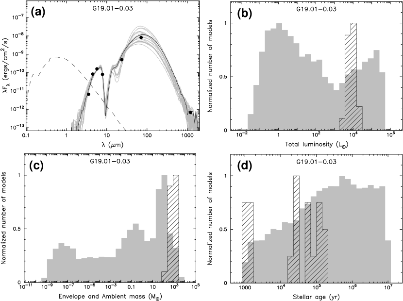
Figure 18: G19.01$-$0.03: (a) Data (black circles) overlaid with the best fit model (solid black line) and other good fits (grey lines) from the Robitaille et al. (2007) model grid. The twenty best fits are shown. The dashed line shows the stellar photosphere, in the absence of circumstellar dust, of the central source for the best-fit model. Histograms of (b) the bolometric luminosity, (c) the envelope mass, and (d) the stellar age for the 20 best-fit models (hatched histograms) and all models in the grid (grey histograms).

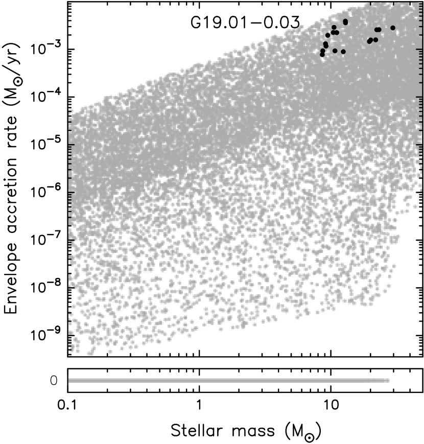
Figure 19: G19.01$-$0.03: Envelope accretion rate v. stellar mass for the 20 best-fit models (black dots) and all models in the grid (grey dots).

The EGO G19.01$-$0.03 is unusual in that the “central” source is clearly resolved from the extended emission in IRAC images (unlike most EGOs), and is a GLIMPSE point source (see also Cyganowski et al., 2008). SED modeling can thus be used to infer the properties of the source driving the 4.5 $\mu$m outflow. As for G11.92$-$0.61, we measured the 70 $\mu$m flux density of G19.01$-$0.03 from the MIPSGAL image. We find a flux density of 223 Jy, with an estimated uncertainty of 50%. Using this measurement, GLIMPSE catalog photometry for the point source SSTGLMC G019.0087-00.0293, the 24 $\mu$m flux density from Cyganowski et al. (2009), and the 1.3 mm flux density from Table 2, we fit the SED using the Robitaille et al. (2007) model fitter. As shown in Figures 18-19, the SED is well-fit (Fig. 18a) by models with bolometric luminosity of $\sim$10⁴ L_⊙ (Fig. 18b), stellar mass $\sim$10 M_⊙ (Fig. 19), envelope mass $\sim$10³ M_⊙ (Fig. 18c), and envelope accretion rate $\sim$10^-3 M_⊙ yr^-1 (Fig. 19). Stellar age is also a parameter of the models, but is not well-constrained (Fig. 18d). In the scheme of Robitaille et al. (2006), evolutionary stage is defined by the ratio of the envelope accretion rate to the stellar mass. The youngest sources, Stage 0/I, are defined as having Ṁ_env/M${}_{*}>$10^-6 yr^-1. For G19.01$-$0.03, Ṁ_env/M_∗$\sim$10^-4 yr^-1 (Fig. 19), indicating that the source is likely to be very young.

4.1.2 Temperature Estimates from Line Emission

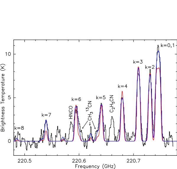
Figure 20: SMA CH₃CN(12-11) spectrum towards the G11.92$-$0.61-MM1 continuum peak (black histogram) overlaid with the best-fit one component (red line) and two component (blue line) models. The physical parameters of the best-fit models are summarized in Table 5. For the single component model, $\Delta$v_FWHM=6 km s^-1; for the two component model, $\Delta$v_FWHM(cool)=7 km s^-1and $\Delta$v_FWHM(warm)=6 km s^-1. For all components, $v_{LSR}$=35.5 km s^-1. The CH₃CN model accounts for emission from CH${}_{3}^{13}$CN, assuming CH${}_{3}^{12}$C:CH${}_{3}^{13}$C=60:1. The strongest observed CH${}_{3}^{13}$CN lines, including those blended with the CH₃CN k=5 and k=6 components, are indicated. The C₂H₅CN line at 220.661 GHz is not fit, nor is the HNCO line at 220.585 GHz (partially blended CH₃CN k=6).

The J=12-11 CH₃CN ladder is well-suited for measuring the gas temperature in hot cores (e.g. Pankonin et al., 2001; Araya et al., 2005; Zhang et al., 2007; Qiu & Zhang, 2009). Figures 20 and  21 show the best-fit single-component model of the CH₃CN emission overlaid on the observed spectrum at, respectively, the G11.92$-$0.61-MM1 and G19.01$-$0.03-MM1 continuum peak. For each CH₃CN emission component, the model assumes local thermodynamic equilibrium (LTE) and the same excitation conditions for all K components, and accounts for optical depth effects and emission from the isotope CH${}_{3}^{13}$CN. The velocity (frequency) separations of the K components are fixed to the laboratory values. The temperature, size (diameter), and CH₃CN column density of the emitting region are free parameters, and the model that best fits the observed spectrum is found by minimizing the mean squared error. The parameters of the best-fit models are summarized in Table 5.

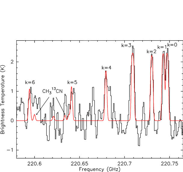
Figure 21: SMA CH₃CN(12-11) spectrum towards the G19.01$-$0.03-MM1 continuum peak (black histogram) overlaid with the best-fit single component model ( red line). The physical parameters of the best-fit model are summarized in Table 5.

A single-component model provides an adequate fit to the CH₃CN spectrum of G19.01$-$0.03-MM1 (Fig. 21; T$\sim$114 K, size$\sim$2500 AU). In contrast, a single-component model is a notably poor fit to the CH₃CN spectrum of G11.92$-$0.61-MM1 (Fig. 20). In particular, the model severely underpredicts the emission from the k=7 and the (blended) k=0/1 lines, while overpredicting the emission from most of the intermediate k components (k=3,4,6). To investigate this discrepancy, we allowed for two CH₃CN-emitting regions, with different temperatures, sizes, and column densities. As shown in Figure 20, a two-component model that includes a compact ($\sim$2300 AU), warm ($\sim$166 K) component and an extended ($\sim$11400 AU), cool ($\sim$77 K) component provides a much better fit to the data (see also Table 5). This combination of parameters is likely not unique, and certainly we expect that the real emission exhibits a gradient in temperature rather than a step function. Even so, this result convincingly demonstrates that both cool and warm temperatures are present. Interestingly, the physical scale of the warm component ($\sim$2300 AU) agrees remarkably well with that of CH₃CN-emitting region in G19.01$-$0.03-MM1 ($\sim$2500 AU).

Five transitions of CH₃OH are detected towards the G11.92$-$0.61-MM1 continuum peak, with E_upper=40-579 K. This is sufficient to obtain an independent estimate of the gas temperature by applying the rotation diagram method (e.g. Goldsmith & Langer, 1999) to the observed CH₃OH emission, using the relations:

$${\frac{N_{u}}{g_{u}}}={\frac{3k}{8\pi^{3}\nu g_{I}g_{K}}}{\frac{1}{\mu^{2}S}}\int{Tdv},$$ (1)

and

$$log(N_{u})/(g_{u})=log(N_{tot}/Q(T_{rot}))-0.4343E_{u}/kT_{rot},$$ (2)

where N_u is the column density in the upper state, k is Boltzmann’s constant, $\nu$ is the line rest frequency, g_I is the nuclear spin degeneracy, g_K is the K degeneracy, $\mu^{2}$S is the product of the square of the molecular dipole moment and the line strength, $\int{Tdv}$ is the observed integrated intensity of the line, N_tot is the total column density, Q(T_rot) is the partition function evaluated at the rotation temperature T_rot, and E_u is the upper state energy of the transition. For each transition, the integrated line intensity was determined from a single Gaussian fit to the line emission at the 1.3 mm continuum peak (Table 3). Both A and E transitions are included in the rotation diagram analysis; we do not detect enough transitions to treat the two types separately. The rotation temperature derived from a weighted least-squares fit to the data is 230$\pm$39 K (Fig. 22), somewhat higher than the temperature derived from the CH₃CN fitting.

As discussed in detail in Goldsmith & Langer (1999), however, optical depth effects can inflate the temperature derived from a rotation diagram analysis. We follow the procedure of Brogan et al. (2007, 2009) in iteratively solving for the values of $\tau$ and T_rot that best fit the data ($C_{\tau}[i]=\tau[i]/(1-e^{\tau[i]})$ where i refers to the ith spectral line). As shown in Figure 22, this improves the fit considerably. The optical depth in the line with the highest opacity (CH₃OH(8_-1,8-7_0,7) at 229.759 GHz) is 3.67. With the optical depth correction, the derived temperature is 166$\pm$19 K. This is in remarkably good agreement with the temperature of the warm component from the CH₃CN analysis (166 K). Only three CH₃OH transitions (E_upper 40-97 K) are detected towards G19.01$-$0.03-MM1, too few for accurate rotation diagram analysis, but consistent with the cooler temperature derived for this source from CH₃CN.

4.1.3 Mass Estimates from the Dust Emission

At millimeter wavelengths, thermal emission from dust and free-free emission from ionized gas can both contribute to the observed continuum flux. For our target EGOs, the available limits on any free-free contribution are not very stringent. Neither G11.92$-$0.61 nor G19.01$-$0.03 had detectable 44 GHz continuum emission in the VLA observations of Cyganowski et al. (2009). The 5$\sigma$ limits are 7 mJy beam^-1 (synthesized beam 0$\farcs$99$\times$0$\farcs$44) and 5 mJy beam^-1 (synthesized beam 0$\farcs$69$\times$0$\farcs$51) respectively. Extrapolating the 5$\sigma$ 44 GHz upper limits assuming optically thin free-free emission ($S_{\nu}\propto\nu^{\alpha}$, $\alpha$=-0.1) gives upper limits at 1.3 mm of 6.0 mJy for G11.92$-$0.61 and 4.3 mJy for G19.01$-$0.03. For the adopted dust temperatures for G11.92$-$0.61-MM1 and G19.01$-$0.03-MM1, a free-free contribution at this level would have a minimal impact on the mass estimates ($\lesssim$0.4 M_⊙). If we instead extrapolate the 5$\sigma$ 44 GHz upper limits assuming a spectral index $\alpha$=1 (appropriate for a hypercompact (HC) HII region, e.g. Kurtz, 2005), the effect on the mass estimates is more substantial, up to $\sim$2.5 M_⊙. For the weakest mm continuum source, G11.92$-$0.61-MM3, free-free emission from a HC HII region ($\alpha$=1) could in principle account for the entirety of the 1.4 mm flux density observed with CARMA and the majority ($\sim$73%) of the 1.3 mm flux density observed with the SMA. Deep, high-resolution continuum data at a range of cm wavelengths are required to constrain the presence and properties of any ionized gas associated with our target EGOs. In the absence of available evidence to the contrary, we assume the entirety of the millimeter-wavelength continuum emission is attributable to thermal emission from dust.

Table 6 presents estimates from the thermal dust emission for the gas mass M_gas, column density of molecular hydrogen N${}_{H_{2}}$, and volume density of molecular hydrogen n${}_{H_{2}}$, for G11.92$-$0.61-MM1, MM2, and MM3 and G19.01$-$0.03-MM1. The gas masses are calculated from:

$$M_{gas}={\frac{4.79\times 10^{-14}RS_{\nu}(Jy)D^{2}(kpc)C_{\tau_{dust}}}{B(\nu,T_{dust})\kappa_{\nu}}},$$ (3)

where R is the gas-to-dust mass ratio (assumed to be 100), S_ν is the integrated flux density from Table 2, D is the distance to the source, C${}_{\tau_{dust}}$ is the correction factor for the dust opacity $C_{\tau_{dust}}=\tau_{dust}/(1-e^{\tau_{dust}})$, B($\nu,T_{dust}$) is the Planck function, and $\kappa_{\nu}$ is the dust mass opacity coefficient in units of cm² g^-1. For gas densities of 10⁶-10⁸ cm^-3, $\kappa_{1.3mm}$$\sim$1 for dust grains with thick or thin ice mantles (Ossenkopf & Henning, 1994). Scaling from $\kappa_{1.3mm}$=1 assuming $\beta$=1.5, we adopt $\kappa_{3.4mm}$=0.24. We estimate a range of dust temperatures for each source based on its observed spectral line properties (discussed in detail below). The dust opacity, ${\tau_{dust}}=-\ln(1-\frac{T_{b}}{T_{dust}})$, is derived using the beam-averaged brightness temperature ($T_{b}$) and assumed dust temperature ($T_{dust}$) for each source and listed in Table 6. The calculated values of $\tau_{dust}$ are generally small ($<$0.1), indicating that the dust emission is optically thin. The column densities and volume densities presented in Table 6 are also beam-averaged values.

As noted above, estimating gas masses using equation 3 requires an estimate of the dust temperature. For G11.92$-$0.61-MM1 and G19.01$-$0.03-MM1 we use the values of T_gas derived from the CH₃CN and CH₃OH emission (§4.1.2). At the high gas densities implied by our observations ($\gtrsim$10⁶ cm^-3), the gas and dust temperatures are expected to be well-coupled (e.g. Ceccarelli et al., 1996; Kaufman et al., 1998). For G11.92$-$0.61-MM1, the situation is complicated by the presence of two temperature components, implied by the CH₃CN fits (§4.1.2). Both the compact warm (size $\sim$0$\farcs$6) and more extended cool (size $\sim$3$\farcs$0) emission regions are similar in scale to the 3$\farcs$2 $\times$ 1$\farcs$8 SMA beam. A step-function temperature structure is physically unrealistic, but the sensitivity and spatial resolution of the present observations are insufficient to resolve the temperature gradient in MM1. In the future, the sensitivity and high spatial resolution attainable with ALMA will allow detailed investigation of the temperature structure. Since the observed millimeter continuum is likely a mix of emission from the warm and cool components, we adopt a broad temperature range (70-190 K) for the estimates in Table 6.

Constraining the temperatures of G11.92$-$0.61-MM2 and G11.92$-$0.61-MM3 is more difficult because of the paucity of associated line emission. MM2 lacks clear MIR counterparts at 3.6-24 $\mu$m, is completely devoid of mm-wavelength line emission, and has no known maser emission. In contrast, MM3 emits at 24 $\mu$m and is associated with 6.7 GHz Class II CH₃OH masers and possibly with a C¹⁸O clump. MM3 is also associated with the brightest 8 $\mu$m emission in the region (Fig. 1a,b). Taken together, the evidence strongly suggests that MM3 is warmer than MM2. For MM2, we adopt a temperature range T_dust=20-40 K based on the absence of associated molecular line emission. The 6.7 GHz CH₃OH masers associated with MM3 are quite weak (peak T_b$\sim$16500 K, 1$\farcs$94 $\times$ 0$\farcs$96 synthesized beam), as are the CH₃OH masers associated with MM1 (peak T_b$\sim$7400 K, Cyganowski et al., 2009). Class II CH₃OH masers are radiatively pumped by infrared photons emitted by warm dust (e.g. Cragg et al., 2005). Cragg et al. (1992) found that a blackbody with T$<$50 K was sufficient to excite moderate 6.7 GHz CH₃OH maser emission (T${}_{b}<$6$\times$10⁴ K). More detailed investigations of Class II CH₃OH maser excitation have focused primarily on the parameter space that gives rise to bright (T${}_{b}>$10⁴ K) maser emission (e.g. Cragg et al., 2005, who invoke dust temperatures $>$100 K). No high-excitation molecular lines (E_upper$>$100 K) are observed towards MM3. In sum, the multiwavelength data suggest two possibilities: MM3 may be of intermediate temperature, or may be hotter (and more evolved) and simply have very little molecular material left around it. Additional data are required to constrain the nature and evolutionary state of MM3 (§4.3.2); we adopt a range of T_dust=30-80 K for the estimates in Table 6.

The physical parameters listed in Table 6 can be calculated from two independent datasets for each core (SMA 1.3 mm and CARMA 1.4 mm for G11.92$-$0.61, SMA 1.3 mm and CARMA 3.4 mm for G19.01$-$0.03). For each compact millimeter continuum source in Table 6, the mass estimate derived from the lower resolution dataset is greater than that derived from the higher resolution dataset. Conversely, a larger beam-averaged column density and volume density are calculated from the higher resolution data. These trends are consistent with the lower-resolution data being more sensitive to emission on larger spatial scales. We note that the mass estimates derived from the dust continuum emission include only circum(proto)stellar material, and not the mass of any protostar or ZAMS star that has already formed within a compact core.

For comparison, Table 5 presents estimates of N(H₂), n(H₂), and M_gas derived from the best-fit source size and CH₃CN column density for the hot cores G11.92$-$0.61-MM1 and G19.01$-$0.03-MM1. Estimates are presented for CH₃CN/H₂ abundances of 10^-7, 10^-8, and 10^-9. Values for the abundance of CH₃CN/H₂ in hot cores reported in the literature span at least an order of magnitude, from $\sim$10^-8-10^-7 (Remijan et al., 2004; Zhang et al., 2007; Bisschop et al., 2007). Lower abundances ($\sim$10^-9) may also be possible even at relatively high temperatures ($>$100 K) in massive hot cores, depending on the warm-up timescale driving the gas-grain chemistry (Garrod et al., 2008). Given the uncertainty in the CH₃CN abundance, the gas mass estimates derived from the CH₃CN emission (Table 5) and from the millimeter dust continuum emission (Table 6) are broadly consistent.

4.1.4 Nature of the Continuum Sources

In summary, the millimeter continuum sources G11.92$-$0.61-MM1, G11.92$-$0.61-MM2, and G19.01$-$0.03-MM1 are dominated by thermal dust emission. The circum(proto)stellar gas masses of these cores range from $\sim$8-62 M_⊙ (based on the SMA data, resolution $\sim$3$\times$2^′′). G11.92$-$0.61-MM1 and G19.01$-$0.03-MM1 are hot cores, with derived gas temperatures of 166$\pm$ 20 K and 144$\pm$ 15 K, respectively. SED modeling indicates that a central (proto)star of $\sim$10 M_⊙ is present within the G19.01$-$0.03-MM1 core. The properties of individual members of the G11.92$-$0.61 (proto)cluster cannot be constrained by this method, as the sources MM1, MM2, and MM3 are unresolved in available data at wavelengths $<$ 1.3 mm. However, the bolometric luminosities of G19.01$-$0.03 and of the G11.92$-$0.61 (proto)cluster as a whole are comparable ($\sim$10⁴ L_⊙). The nature of G11.92$-$0.61-MM3 is less clear. In principle, an HCHII region undetected in previous observations could account for the majority of the G11.92$-$0.61-MM3 mm flux density (§4.1.3), but additional observations at cm wavelengths are needed to investigate this possibility. If the mm flux density of G11.92$-$0.61-MM3 is dominated by dust emission, the compact gas mass is $\sim$3-9 M_⊙, the lowest of the observed cores. The relative evolutionary states of the members of the G11.92$-$0.61 (proto)cluster, and of G11.92$-$0.61 and G19.01$-$0.03, are discussed further in §4.3.2.

Based on the SMA 1.3 mm data, the total mass in compact cores is $\sim$37-94 M_⊙ in G11.92$-$0.61 and $\sim$12-16 M_⊙ in G19.01$-$0.03. Additional low-mass sources may also be present, but undetected in our observations; the 5$\sigma$ sensitivity limit of the SMA data corresponds to a mass limit of a few M_⊙ for moderate dust temperatures (Table 6). Schuller et al. (2009) calculate a mass for the larger-scale (40$\times$34^′′) G19.01$-$0.03 gas/dust clump of 1070 M_⊙, based on ATLASGAL 870 $\mu$m data and an NH₃ T_kin of 19.5 K. This suggests that only $\sim$1% of the total mass is in the compact core we observe with the SMA, and a considerable reservoir of material is in an extended envelope that is mostly resolved out in the continuum as in the ¹²CO line emission (§3.2.4). The compact cores in the G11.92$-$0.61 protocluster constitute a larger percentage of the total mass reservoir. From the 850 $\mu$m SCUBA flux (12 Jy, Walsh et al., 2003), we estimate a total mass for the clump of $\sim$780 M_⊙ for T_dust=20 K (typical of the NH₃ temperatures reported for ATLASGAL sources by Schuller et al., 2009) and $\kappa_{850\mu m}$=2.2 (interpolated from the values tabulated by Ossenkopf & Henning, 1994). Based on this estimate, the compact SMA cores in G11.92$-$0.61 comprise $\sim$5-12% of the total mass, with a remaining large-scale gas reservoir of several hundred M_⊙ for the G11.92$-$0.61 (proto)cluster.

Single dish surveys of massive star forming regions have revealed spectroscopic signatures of parsec-scale infall in cluster forming environments (e.g. Wu & Evans, 2003). In addition, new high resolution observations of the G20.08$-$0.14 N cluster detect infall at the scale of both cluster forming clumps and massive star forming cores, all part of a continuous, hierarchical accretion flow (Galván-Madrid et al., 2009). Recent simulations also indicate the importance of accretion from large-scale gas reservoirs in massive star and cluster formation, particularly for determining the final stellar masses (Smith et al., 2009; Peters et al., 2010; Wang et al., 2010). Since the presence of an active outflow indicates ongoing accretion, the masses of the members of the G11.92$-$0.61 (proto)cluster may grow significantly with time. For G19.01$-$0.03, the SED modeling is consistent with a central YSO of mass $\sim$10 M_⊙ that is actively accreting at a rate of $\sim$10^-3 M_⊙ year^-1. This central source is associated with a compact gas and dust core of mass $\sim$12-16 M_⊙. However, with a substantial ($\sim$1000 M_⊙) extended reservoir of material from which to draw, the final mass of G19.01$-$0.03 may be substantially higher.

4.2 Outflows

A single dominant bipolar molecular outflow is associated with each of our targeted EGOs. These outflows are traced by high-velocity, well-collimated ¹²CO(2-1) and HCO⁺(1-0) emission. In both EGOs, the red and blue outflow lobes clearly trace back to a driving source identified with a compact mm continuum core (Figs. 6, 13). This relative clarity is somewhat unusual. In many massive star-forming regions, multiple outflows are observed, with complex kinematics that can make it difficult to identify driving source(s) (Zhang et al., 2007; Shepherd et al., 2007; Brogan et al., 2009). Indeed, since YSOs of all masses drive bipolar molecular outflows during the formation process (e.g. Richer et al., 2000), one would expect multiple outflows in a protocluster such as G11.92$-$0.61.

A second outflow may indeed be present in G11.92$-$0.61. Blueshifted ¹²CO(2-1), HCO⁺(1-0),and SiO(2-1) emission are present NE of the mm continuum cores, and redshifted emission to the SW (§3.1.4). This is opposite the velocity gradient of the dominant outflow, and this emission may trace a second outflow. If so, the driving source is likely the continuum source MM3, which is approximately equidistant between the two lobes (Fig. 6c; the possible second outflow is most prominent at moderate velocities, see also §3.1.4). Alternatively, the observed morphology may be attributable to orientation effects. An outflow nearly in the plane of the sky may appear to have overlapping red and blue-shifted lobes (e.g. Cabrit & Bertout, 1990). Another possible explanation is outflow precession. For an outflow axis close to the plane of the sky, precession can produce the appearance of inversions between blue/red-shifted emission along the outflow axis (e.g. Beuther et al., 2008), such as the pattern seen in G11.92$-$0.61. In addition, the ¹²CO and HCO⁺ data hint at the possible presence of a third, low-velocity outflow along a SE-NW axis. As shown in Figures 7-8, moderately redshifted gas is present SE of the continuum sources, and moderately blueshifted gas to the NW (26.7, 39.9, and 46.5 km s^-1 panels). The interpretation of this emission as an outflow is, however, very uncertain. The moderate-velocity ¹²CO emission appears to correlate with extended 4.5 $\mu$m emission and 44 GHz CH₃OH masers, but the HCO⁺ emission (which is subject to less spatial filtering) is much more extended, suggesting confusion with the ambient cloud, and the SiO(2-1) emission (Fig. 9) does not show the same velocity pattern. There is no clear evidence in our data for an outflow driven by the continuum source MM2.

4.2.1 Outflow Properties

We estimate the physical properties of the molecular outflows in G11.92$-$0.61 and G19.01$-$0.03 independently from the SMA ¹²CO(2-1) and the CARMA HCO⁺(1-0) data. As discussed in §3.1.4 and §3.2.4, outflow gas is confused with diffuse emission from the surrounding cloud at velocities near the source $v_{LSR}$. This problem is particularly acute for ¹²CO, because of its high abundance. To avoid including contributions from the ambient cloud, we consider only high velocity gas in our estimates of the outflow physical properties (Table 7). To further isolate the outflow gas, a polygonal mask is defined for each red or blueshifted outflow lobe in Figures 6 and  13. The polygonal masks are drawn to encompass all outflow emission in the integrated intensity images of the high-velocity gas, and checked against the datacubes. The appropriate mask is applied to each channel in which the outflow dominates over emission from the ambient cloud. Assuming optically thin emission, the gas mass of the outflow is then calculated from

$$M_{out}={\frac{1.186\times 10^{-4}Q(T_{ex})e^{\frac{E_{upper}}{T_{ex}}}D^{2}\int S_{\nu}dv}{\nu^{3}\mu^{2}S\chi}}$$ (4)

where M_out is the outflow gas mass in M_⊙, T_ex is the excitation temperature of the transition in K, Q(T_ex) is the partition function, E_upper is the upper energy level of the transition in K, $\nu$ is the frequency of the transition in GHz, $\chi$ is the abundance of the observed molecule relative to H₂, D is the distance to the source in kpc, and $S_{\nu}$ is the line flux in Jy. Following Qiu et al. (2009), for ¹²CO we adopt an abundance ($\chi$) relative to H₂ of 10^-4, an excitation temperature of 30 K, and a mean gas atomic weight of 1.36 (included in the constant in equation (1)). For HCO⁺, we adopt the same excitation temperature (T_ex=30 K), and an abundance of 10^-8 relative to H₂ (Vogel et al., 1984; Rawlings et al., 2004; Klaassen & Wilson, 2007). We use Q(30 K)=11.19 for ¹²CO and Q(30 K)=14.36 for HCO⁺, interpolating from the values provided in the Cologne Database for Molecular Spectroscopy (CDMS, Müller et al., 2001; Müller et al., 2005) and $\mu^{2}$S=0.02423 debye² for ¹²CO(2-1) and $\mu^{2}$S=15.21022 debye² for HCO⁺(1-0) from the Splatalogue spectral line database. Following Qiu et al. (2009), we estimate the outflow momentum and energy using

$$P_{out}=\Sigma M_{out}(\Delta v)\Delta v$$ (5)

and

$$E_{out}={\frac{1}{2}}\Sigma M_{out}(\Delta v)(\Delta v)^{2}$$ (6)

where M_out($\Delta$v) is the outflow mass in a given channel and $\Delta$v =$|$v${}_{center,channel}-$$v_{LSR}$$|$. For these calculations, we adopt $v_{LSR}$=35 km s^-1 for G11.92$-$0.61 and $v_{LSR}$=60 km s^-1 for G19.01$-$0.03. We estimate the dynamical timescale from $t_{dyn}=L_{outflow}/v_{max}$ where the length L_outflow and the maximum velocity v_max are determined separately for the red and blue lobes of each outflow (Table 7). In estimating L_outflow, we measured the extent of the red/blueshifted emission from the driving mm continuum source. For G11.92$-$0.61, we assumed that the main outflow was driven by MM1, and the possible second (“northern”) outflow by MM3. Using the dynamical timescales, we also estimate the mass and momentum outflow rates, Ṁ${}_{out}=M_{out}/t_{dyn}$ and Ṗ${}_{out}=P_{out}/t_{dyn}$. For each outflow, the outflow parameters are listed in Table 7, along with the velocity ranges used. For G19.01$-$0.03, the “NE blue clump” (Table 7) is the easternmost knot of blueshifted ¹²CO emission (Fig. 13a). This knot is offset from the main ¹²CO jet, and a separate mask was defined for it. However, the HCO⁺ and SiO morphology indicate that this ¹²CO emission is likely part of the outflow, so we include it in our estimates of the outflow properties.

Several salient points are reflected in Table 7: (1) channels nearest the systemic velocity disproportionately affect the outflow mass estimates; (2) the estimates derived from HCO⁺ and ¹²CO observations differ by approximately an order of magnitude; and (3) there is considerable uncertainty in the estimate of the dynamical timescale, and hence of the mass and momentum outflow rates. Each of these points is discussed in more detail below.

As noted above, dominant, unconfused outflow emission is the primary criterion for choosing the velocity (channel) ranges over which to integrate outflow mass, momentum, and energy. In general, column densities are highest near the systemic velocity of a cloud. As a result, estimates of outflow mass and other properties are extremely sensitive to how closely the velocities considered approach the $v_{LSR}$, e.g. to the minimum value of $\Delta$v=$|$v${}_{center,channel}-$$v_{LSR}$$|$. For this reason, where practicable we choose velocity ranges such that min.($\Delta$v_blue)$\sim$min.($\Delta$v_red) and used the same velocity range for ¹²CO and HCO⁺ mass estimates. In G19.01$-$0.03, it is possible to follow the outflow much closer to the systemic velocity in HCO⁺(1-0) than in ¹²CO(2-1), with minimal confusion from ambient diffuse gas. As an illustrative example, in Table 7 we present estimates of the G19.01$-$0.03 outflow properties derived from HCO⁺ using velocity ranges beginning $\sim$$\pm$6km s^-1, $\pm$8km s^-1, and $\pm$10km s^-1 from the systemic velocity. The difference in the estimated total outflow mass (and consequently in Ṁ_out) is about a factor of 2. The estimates of the outflow momentum, energy, and momentum outflow rate are less severely affected because the channels in question are near the systemic velocity (low $\Delta$v). In G11.92$-$0.61, the situation is complicated by the possible second outflow, so we restrict the HCO⁺ mass estimates to the same velocity range considered for ¹²CO.

For a given outflow lobe, the mass estimate derived from HCO⁺(1-0) is roughly an order of magnitude larger than that derived from ¹²CO(2-1). There are two possible explanations for this discrepancy: spatial filtering and uncertain HCO⁺ abundance. For the massive outflow in G240.31+0.07 (D=6.4 kpc), Qiu et al. (2009) found that their SMA compact configuration ¹²CO observations recovered $<$10% of the single-dish flux at line center, $\sim$80% in the “line wing” ($\Delta$v$\sim$13 km s^-1), and nearly 100% at more extreme velocities ($\Delta$v$\gtrsim$ 15 km s^-1). Our CARMA HCO⁺ data are more sensitive to larger-scale emission than our SMA ¹²CO data, and the linear resolution of the Qiu et al. (2009) SMA observations is comparable to that of our CARMA EGO data. It is plausible that our CARMA observations are picking up outflow emission on larger spatial scales, to which the SMA is insensitive. In this case, the outflow parameters estimated from the HCO⁺ emission would be more representative of the true outflow properties. If, however, the HCO⁺ abundance in our target EGOs is enhanced above our adopted value of 10^-8, this could lower the mass estimates from the HCO⁺ emission into better agreement with those from ¹²CO. Modeling by Rawlings et al. (2004) found best-fit HCO⁺ abundances of 10^-10 in the envelope, 10^-9 in the jet/cavity, and 10^-7 in the boundary layer, though the models were optimized for the low-mass source L1527. Moderate optical depth corrections would also increase the ¹²CO mass estimates (see below), bringing them into better agreement with those from HCO⁺.

There is considerable ambiguity in the determination of the dynamical timescale, particularly for asymmetric and/or clumpy outflows such as those observed towards our target EGOs. We have followed other recent high-resolution interferometric outflow studies (e.g. Qiu & Zhang, 2009; Qiu et al., 2009) in defining $t_{dyn}=L_{outflow}/v_{max}$, and calculate t_dyn independently for the red and blue lobes of each outflow. As Table 7 illustrates, these estimates can differ significantly. Some single-dish studies instead use $t_{dyn}=R/V$, where R is the distance between the peaks of the red and blue outflow lobes, and V is the mean outflow velocity, calculated as the outflow momentum divided by the outflow mass (P/M, e.g. Zhang et al., 2005). Both approaches assume, however, that an outflow (or an outflow lobe) can be well-characterized by a single velocity. The G19.01$-$0.03 outflow is clumpy, and characterized by discrete knots of high velocity gas. If $t_{dyn}=L_{knot}/v_{max,knot}$ is calculated individually for each of the three blueshifted knots in Figure 13a, the values are (from north to south) $\sim$3600 years, 1100 years, and 600 years. This range suggests the limitations of attempting to evaluate the age of a flow using a single velocity. Estimating t_dyn is further complicated by the unknown effects of ambient density and inclination angle. The expressions for t_dyn above assume free expansion. Finally, the inclination of the outflows is unknown. The extended morphologies of the 4.5 $\mu$m emission and the high-velocity molecular gas in our target EGOs suggest that the outflows may lie near the plane of the sky (Figs. 6, 13). However, intermediate inclination angles are also plausible, since the red and blueshifted outflow lobes are spatially distinct, particularly in G19.01$-$0.03 (e.g. Cabrit & Bertout, 1990), and very high velocity gas ($\sim$60 km s^-1 from $v_{LSR}$ in G11.92$-$0.61 and $>$100 km s^-1 from $v_{LSR}$ in G19.01$-$0.03) is observed. Table 7 presents estimates of outflow parameters without correction for inclination, and for $\theta$=10^∘, 30^∘, and 60^∘, where $\theta$ is the inclination angle of the outflow to the plane of the sky. In the extreme case of $\theta$=10^∘, correcting for inclination increases the estimated Ṁ_out and P_out by a factor of $\sim$6, and Ṗ_out and E_out by a factor of $\sim$30. For an intermediate inclination $\theta$=30^∘, the increases are more moderate: a factor of $\sim$2 for Ṁ_out and P_out, and $\sim$4 for Ṗ_out and E_out. For outflows in which the red and blue lobes give very different estimates of t_dyn, Table 7 presents estimates of Ṁ_out and Ṗ_out for the outflow as a whole using an intermediate timescale. In calculating Ṁ_out and Ṗ_out from the HCO⁺ data we adopt the dynamical timescales calculated from ¹²CO, since the highest velocity outflow gas extends beyond the limited velocity coverage of the CARMA observations.

In general, our estimates of outflow mass are lower limits, and likely extreme lower limits. As a result, the other physical parameters (which depend on the outflow mass) will also be underestimated. There are three main contributing factors: (1) extended emission missed by the interferometers; (2) outflow emission near the systemic velocity excluded by our conservative velocity cuts; and (3) the assumption of optically thin emission. Our estimates of the outflow mass assume optically thin emission in both ¹²CO(2-1) and HCO⁺(1-0). While this assumption is likely valid for HCO⁺, it is more problematic for ¹²CO, and some recent interferometric outflow studies have made detailed corrections for ¹²CO optical depth (e.g. Qiu et al., 2009). Because we were conservative in selecting the velocity ranges over which to calculate outflow parameters, significant ($\geq$5$\sigma$) ¹³CO(2-1) emission is detected in only one channel that contributes to the estimates presented in Table 7, for one outflow: the main outflow in G11.92$-$0.61 (v=48.1 km s^-1). If we calculate the ¹²CO/¹³CO line ratio at the ¹³CO peak in this channel, the implied optical depth correction factor is $\sim$6.7 for a ¹²CO/¹³CO abundance ratio of 40 (for a Galactocentric distance of 4.7 kpc, Wilson & Rood, 1994). Applying this factor would increase the contribution of this single channel to the outflow mass from $\sim$0.07 M_⊙ to $\sim$0.5 M_⊙, the mass of the red outflow lobe from $\sim$0.2 to $\sim$0.6 M_⊙, and the total mass of the outflow from $\sim$0.8 M_⊙to $\sim$1.2 M_⊙. Applying this single correction factor, however, would likely result in an overestimate. The correction factors derived at two other positions in the outflow with detected ¹³CO emission are more modest ($\sim$3 and 4.5, see also Cabrit & Bertout, 1990). The signal-to-noise of the ¹³CO data are not sufficient to accomodate attempting an opacity correction as a function of position, particularly given the overwhelming lack of detected ¹³CO emission in the other channels considered. By assuming optically thin emission, our mass estimates based on ¹²CO will definitively be lower limits, without the ambiguity of possibly overcorrecting.

We do not estimate outflow parameters from the SiO(2-1) emission observed with CARMA because of the uncertainty in the SiO abundance in the emitting region. Values in the literature for the SiO abundance in molecular outflows and massive star-forming regions vary over at least two orders of magnitude (from $\sim$10^-6 to 10^-8, Pineau des Forets et al., 1997; Caselli et al., 1997; Schilke et al., 1997). Models indicate that the SiO abundance depends sensitively on the shock conditions (including velocity, ambient density, and time since the passage of the shock, Pineau des Forets et al., 1997; Schilke et al., 1997), which are not constrained by our single-transition SiO observations. Since our CARMA data show that the SiO emission is extended well beyond the beamsize of the JCMT SiO(5-4) spectra (§3.1.1,§3.2.1), we cannot constrain the physical conditions in the SiO emitting gas.

4.2.2 Comparison with Other Objects

Properties of outflows from MYSOs reported in the literature, based on high angular resolution observations, range over several orders of magnitude. As indicated by the discussion above, some of this range may be attributable to differences in spatial filtering and to the (large) uncertainties inherent in assuming tracer abundances and correcting (or not) for optical depth and inclination effects. At the low end, Qiu & Zhang (2009) calculate M_out of 0.22 M_⊙, P_out of 4.9 M_⊙ km s^-1, Ṁ_out of 10^-4 M_⊙ yr^-1, and Ṗ_out of 2.2$\times$10^-3 M_⊙ km s^-1 yr^-1 based on SMA ¹²CO data for the extremely high velocity outflow in HH80-81 (D=1.7 kpc). At the high end, outflow masses of several tens (27 M_⊙, IRAS 18566+0408, D=6.7 kpc: Zhang et al., 2007) to $\gtrsim$ 100 M_⊙ (98 M_⊙, G240.31+0.07, D=6.4 kpc; 124 M_⊙, Orion-KL: Qiu et al., 2009; Beuther & Nissen, 2008) have been reported. These studies, however, use tracers with uncertain abundance in outflows (SiO; Zhang et al., 2007), or combine single dish and interferometric data (Qiu et al., 2009; Beuther & Nissen, 2008). Also, except for Orion-KL, the estimated dynamical timescales for these more massive outflows are longer ($>$10⁴ years), so the estimated mass outflow rates, Ṁ_out, are still only a few $\times$ 10^-3 M_⊙ yr^-1. The estimated parameters of the molecular outflows in our target EGOs (Table 7) are roughly in the middle of the range reported in the literature. The main outflow in G11.92$-$0.61 and the outflow in G19.01$-$0.03 have broadly similar characteristics: each has t_dyn of a few $\times 10^{3}$ years, and (based on the HCO⁺ data) M_out of a few M_⊙, P_out of a few hundred M_⊙ km s^-1, E_out of tens to a hundred $\times 10^{45}$ ergs, Ṁ_out of a few $\times 10^{-3}$ M_⊙ yr^-1, and Ṗ_out of a few hundredths to one M_⊙ km s^-1 yr^-1 (the estimates of E_out and Ṗ_out are most severely affected by the uncertainty in the inclination angle). These parameters are generally comparable to those for the total high-velocity gas (attributed to three separate outflows) in the massive star-forming region IRAS 17233-3606 derived from high-resolution SMA ¹²CO observations by Leurini et al. (2009) (opacity correction applied), though for IRAS 17233-3606 the estimated dynamical timescale is somewhat shorter ($\sim$300-1600 years) than for our target EGOs. The EGO outflow properties are also quite similar to those of the outflows in the AFGL5142 protocluster, as estimated from OVRO HCO⁺(1-0) and SMA ¹²CO(2-1) observations (particularly accounting for the different assumed HCO⁺ abundance, 10^-9; Hunter et al., 1999; Zhang et al., 2007). As noted in §3.1.3, the frequency coverage of the Zhang et al. (2007) SMA data is comparable to that of our observations, and the SMA spectrum of AFGL5142 MM2–the probable driving source of the north-south outflow studied by Hunter et al. (1999)–is very similar to that of G11.92$-$0.61-MM1. Even the least massive outflow observed towards our target EGOs (the “northern outflow” in G11.92$-$0.61) has values of M_out, Ṁ_out, etc. at least an order of magnitude greater than those typical of low-mass outflows observed at high angular resolution(e.g. Arce & Sargent, 2006).

Several large scale single-dish surveys of molecular outflows have shown correlations between the properties of the outflow and those of the driving source (in particular its bolometric luminosity and core mass, e.g. Cabrit & Bertout, 1992; Shepherd & Churchwell, 1996; Hunter, 1997; Beuther et al., 2002), though other recent studies have found considerable scatter and weak or no evidence of any correlations (e.g. Ridge & Moore, 2001; Zhang et al., 2005). The applicability of these relations to parameters derived from interferometric observations is unclear, since, as discussed above, interferometers resolve out a significant fraction of the extended emission and so underestimate the outflow mass and other parameters. The mass and momentum outflow rates for our target EGOs (Table 7) do generally agree, within the considerable scatter, with the Ṁ_out and Ṗ_out expected for a driving source of luminosity $\sim$10⁴ L_⊙ (Ṁ_out $\sim$a few $\times$ 10^-5 to a few $\times$ 10^-3 M_⊙ year^-1, Ṗ_out$\sim$a few $\times$ 10^-3 to 10^-1 M_⊙ km s^-1 year^-1: Cabrit & Bertout, 1992; Shepherd & Churchwell, 1996; Beuther et al., 2002; Zhang et al., 2005). For G11.92$-$0.61 and G19.01$-$0.03, the mass in the outflow (as derived from the HCO⁺ data, Table 7) is roughly comparable to the circum(proto)stellar gas mass of the driving compact millimeter core (Table 6), and, for G19.01$-$0.03, to the mass of the central (proto)star inferred from the SED modeling (§4.1.1). It has been suggested for some time that the mass in MYSO outflows is accumulated from the larger-scale environment (e.g. Churchwell, 1997). Notably, the properties of the outflows in our target EGOs are consistent with the single-dish relations with respect to “core mass” only if the total masses of the single-dish clump (as opposed to the masses of the compact cores resolved with the SMA and CARMA) are considered.

4.3 Diversity within the EGO Sample

Our high resolution mm observations suggest considerable diversity within the EGO sample in the clustering properties and evolutionary states of the outflow driving sources. Since extended 4.5 $\mu$m emission specifically targets a population with ongoing outflow activity and active, rapid accretion, the range in source properties is of interest in the context of recent theoretical work on feedback effects in cluster-scale models of massive star formation (e.g. Krumholz & Matzner, 2009; Bate, 2009; Wang et al., 2010; Peters et al., 2010).

4.3.1 Multiplicity

The EGO G11.92$-$0.61 was chosen as a target for high resolution mm observations in part because its 24 $\mu$m morphology and two associated 6.7 GHz Class II CH₃OH maser spots indicated the possible presence of multiple MYSOs. Our high-resolution SMA and CARMA data indeed reveal three compact millimeter continuum sources associated with the EGO. The clustering scale of these cores is $\sim$0.1 pc, comparable to that in S255N, a massive protocluster that is also associated with a 4.5 $\mu$m outflow (Cyganowski et al., 2007). No additional structure is seen in the CARMA 1.4 mm image (resolution 1$\farcs$44 $\times$ 0$\farcs$87 $\sim$0.03$\times$ 0.02 pc $\sim$5500 $\times$ 3300 AU) as compared to the lower resolution SMA 1.3 mm image (resolution 3$\farcs$2 $\times$1$\farcs$8 $\sim$0.06 $\times$ 0.03 pc $\sim$12000 $\times$ 6800 AU). Further structure may, however, be suggested by the complicated kinematics of the ¹²CO, HCO⁺, and particularly the SiO emission. In NGC6334I(N), a tight ($\sim$800 AU separation) binary is thought to cause the precession of the molecular outflow: both components of the binary are contained within a hot core of diameter $\sim$1400 AU (Brogan et al., 2009). If outflow precession is responsible for the complex velocity structure in G11.92$-$0.61, it would suggest that the outflow driving source, G11.92$-$0.61-MM1, could be an unresolved (proto)binary.

In contrast to G11.92$-$0.61, our interferometric observations of G19.01$-$0.03 reveal only a single continuum source. For G19.01$-$0.03, our SMA 1.3 mm continuum image provides the highest resolution: 3$\farcs$2$\times$1$\farcs$7 $\sim$0.07$\times$0.03 pc $\sim$13400 $\times$7100 AU. This is sufficient to resolve clustering at the scale seen in G11.92$-$0.61 and S255N, though not proto-Trapezia (such as NGC6334I and I(N), Hunter et al., 2006). The CH₃CN(12-11) spectrum of G19.01$-$0.03-MM1 is unusual, in that the k=0, k=1, and k=2 components are nearly equal in strength, and the k=3 component is even stronger (Fig. 21). This is likely indicative of either unresolved multiplicity or unresolved density/temperature gradients, but the current data are insufficient to distinguish between these scenarios.

If G19.01$-$0.03 is truly a single (proto)star, it would be an unusual example of a massive star forming in isolation. Some recent models suggest that an apparently lone MYSO could also be indicative of the very earliest stages of cluster formation. Peters et al. (2010) find that the most massive star begins to grow early in the cluster formation process, and finishes accreting while its surrounding cluster is still forming. Accretion is clearly ongoing in G19.01$-$0.03, and our mm observations provide several other indicators of its youth (§4.3.2). Higher resolution and more sensitive (sub)mm observations of G19.01$-$0.03 are needed to determine whether sub-10000 AU clustering or low-mass (proto)stars are present.

4.3.2 Relative Evolutionary State

The three millimeter continuum sources in the G11.92$-$0.61 (proto)cluster exhibit a range of MIR-mm properties and maser associations, suggestive of a range in mass and/or evolutionary state. The strongest mm continuum source, G11.92$-$0.61-MM1, is a hot core, and the driving source of the dominant bipolar outflow in the region. In contrast, G11.92$-$0.61-MM2 is devoid of millimeter-wavelength line emission, and shows no evidence for associated outflow or maser activity. The gas mass of G11.92$-$0.61-MM2, calculated from its arcsecond-scale thermal dust emission, is $\sim$17-42 M_⊙, sufficient to form an intermediate to high-mass star. The compact gas mass associated with G11.92$-$0.61-MM1 is smaller, $\sim$5-13 M_⊙. This does not, however, include the mass of central (proto)star(s), which the associated MIR and maser emission indicate are likely present. MM2, which exhibits no signs of maser or outflow activity, may be a massive protostellar core. High-resolution observations in a thermometer of cold, dense gas (e.g. NH₃) would help to determine whether this source is internally heated by a central YSO or externally heated by feedback processes in the cluster environment.

The evolutionary state of G11.92$-$0.61-MM3, the weakest millimeter continuum source in the region, is somewhat ambiguous. It is associated with 6.7 GHz Class II CH₃OH maser and 24 $\mu$m emission, and with the strongest 8.0 $\mu$m emission in the region (Fig. 1a,b). The nature of the 8 $\mu$m counterpart is unclear, as it appears somewhat extended and it is possible that H₂ line emission contributes significantly to the broadband flux. Very little compact mm molecular line emission is detected coincident with MM3, and no emission in high excitation (E_upper$>$100 K) molecular lines. Like MM1, the compact gas mass associated with MM3 is relatively small ($\sim$2-6 M_⊙), but the MIR and maser emission suggest that a central (proto)star has likely already formed. De Buizer (2006) suggested that Class II CH₃OH maser emission may be excited in the MIR-bright walls of an outflow cavity. The morphology of the 24 $\mu$m emission, however, appears inconsistent with MM3 being a hotspot on an outflow cavity wall. Another possibility is that MM3 is more evolved, and so has dispersed most of the molecular gas in its immediate vicinity. This would be consistent with its MIR properties. We also note that MM3 is the only compact millimeter continuum source for which the arcsecond-scale 1.4 mm emission observed with CARMA could conceivably be due to a HC HII region that fell below the Cyganowski et al. (2009) 44 GHz continuum detection limit (§4.1.3). High resolution observations over a range of cm wavelengths are required to constrain the evolutionary state of MM3.

Several lines of evidence suggest that G19.01$-$0.03 is younger than the G11.92$-$0.61 massive star-forming region. Compared to G11.92$-$0.61-MM1, the millimeter molecular line emission from G19.01$-$0.03-MM1 is sparse and weak. The relative lack of chemical complexity observed towards G19.01$-$0.03-MM1, and its cooler derived temperature, are both consistent with a less-advanced hot core chemisty (e.g. van Dishoeck & Blake, 1998). There have been a number of suggestions in the literature that the relative abundances of various sulfur-bearing species may provide chemical clocks for hot cores (e.g. Charnley, 1997; Hatchell et al., 1998; Herpin et al., 2009). Transitions of several species invoked in these models fall within the frequency coverage of our SMA observations, namely SO, OCS, and SO₂. Unfortunately, the most diagnostic abundance ratios are those relative to H₂S (e.g. Charnley, 1997), which does not have transitions within our SMA bandwidth.

The calculation and comparison of abundances for the sulfur-bearing species in the EGO hot cores must be regarded with considerable caution. Such comparisons rely on an assumption that all relevant emission arises from the same excitation conditions in the same physical volume of gas. From our data, it is evident that in G11.92$-$0.61 the outflow contributes to the excitation of SO emission, and even the compact OCS emission may have an outflow contribution (§3.1.3). Considering the two-component temperature model required to fit the CH₃CN emission, it is also plausible that the low-excitation SO emission arises from a larger volume than the higher-excitation OCS emission (both unresolved by the SMA beam). Similarly, the thermal dust emission (from which we infer N(H₂)) may arise from a different volume than the molecular line emission. If we nonetheless compute the OCS and SO abundances for G11.92$-$0.61-MM1 assuming T_ex=166 K and N(H₂)=2.7$\times$10²³ cm^-2 (beam-averaged column density for T_dust=166 K and the SMA beam), we find abundances of $\sim$1.9 $\times$ 10^-8 and 1.3 $\times$ 10^-8 relative to H₂, respectively. For G19.01$-$0.03-MM1, (T_ex=115 K, N(H₂)=3.5$\times$10²³ cm^-2, Table 6), we calculate abundances of $\sim$3$\times$10^-9 for OCS and $\sim$6$\times$10^-10 for SO. These estimates correspond to a [SO/OCS] ratio of $\sim$0.2 for G19.01$-$0.03 and $\sim$0.7 for G11.92$-$0.61-MM1, consistent with G19.01$-$0.03 being younger and less evolved (Herpin et al., 2009). Other, more global indicators also point to the relative youth of G19.01$-$0.03 compared to G11.92$-$0.61. Since MYSOs dissipate their natal envelopes as they grow, the presence of an extended envelope is suggestive of youth. Compact mm core(s) account for a smaller fraction of the total clump mass in G19.01$-$0.03 than in G11.92$-$0.61 (§4.1.3), consistent with indications from the ¹²CO emission and SED modeling that G19.01$-$0.03-MM1 is still embedded in a massive ($\sim$1000 M_⊙) large-scale envelope.

4.3.3 Future Work

These initial results demonstrate the potential of the EGO sample for probing the importance of protostellar feedback in the formation of massive stars and star clusters. Recent theoretical work has just begun to include realistic feedback effects in cluster-scale models, including protostellar outflows (Wang et al., 2010), photoionization/HII regions (Peters et al., 2010; Krumholz & Matzner, 2009), and radiative feedback (Bate, 2009). However, current models do not include all feedback mechanisms, and hence do not address the question of which mechanism(s) are most important at which stages of (proto)cluster formation, or of how these mechanisms interact. EGOs are an outflow-selected sample. Hence, characterizing their outflows as well as other possible forms of feedback (ionized jets/winds, gas heating) will help to establish whether there is an outflow-dominated stage of (proto)cluster formation. Addressing this question in a statistically meaningful way will require high resolution (sub)mm wavelength data similar to those presented here for a wide range of EGO sources. High-resolution cm continuum data are also necessary to constrain the presence and physical properties of ionized gas, while cm-wavelength line observations (e.g. of NH₃) are needed to constrain gas temperatures and densities in cool cores that lack mm-wavelength line emission. Accumulating uniform datasets for large samples is essential for comparisons of different objects. The capabilities of the EVLA and ALMA put such surveys within reach, and EGOs will be promising targets for these instruments. One fortunate characteristic of EGOs is the probable 229.759 GHz CH₃OH Class I maser line which we detect toward both objects. These are, to our knowledge, the fifth and sixth reported examples of this maser in the literature, although higher resolution observations are still required to unambiquously confirm the maser nature of the emission based on the brightness temperature. As with the 44 GHz Class I masers, these features may be common in massive star-forming regions. If so, they will be of interest as self-calibration targets to help enable future very high-resolution 1.3 mm observations (e.g. with ALMA).

5 Conclusions

Our high-resolution millimeter observations of two EGOs unambiguously show that they are young MYSOs driving massive bipolar outflows. The spatial coincidence of high velocity ¹²CO(2-1) and HCO⁺(1-0) emission with the extended 4.5 $\mu$m lobes supports the outflow hypothesis for the 4.5 $\mu$m emission. A single dominant outflow is identified in each EGO, with tentative evidence for multiple outflows in one source (G11.92$-$0.61). The morphology and kinematics of the SiO(2-1) emission differ from the other outflow tracers in that some of the strongest red and blueshifted features are offset from the extended 4.5 $\mu$m emission, and may trace the impact of outflow shocks on dense gas in the surrounding cloud. The morphology of the high-velocity gas with respect to 44 GHz Class I CH₃OH maser emission further solidifies the association of this type of maser with outflows. Anomalously intense and narrow components of 229.759 GHz CH₃OH emission are also detected in the outflow lobes from both objects, suggesting additional Class I maser activity. The outflow driving sources appear as compact cores of millimeter continuum emission and dense gas, including the hot core molecules CH₃OH, CH₃CN and OCS. Coincident with 22 GHz water maser emisson, G11.92$-$0.61-MM1 shows considerably richer and stronger hot core line emission than G19.01$-$0.03-MM1, consistent with its warmer temperature derived from the multi-transition analysis of the CH₃CN and CH₃OH emission (166$\pm$20 v. 114$\pm$15 K). Both hot cores exhibit 24 $\mu$m and 70 $\mu$m emission in MIPSGAL images and contain 6.7 GHz Class II CH₃OH masers, all consistent with their identification as MYSOs.

Our observations also reveal considerable diversity within the EGO sample. Although observed at the same spatial resolution, G19.01$-$0.03 appears as a single MYSO while G11.92$-$0.61 resolves into a cluster of three compact dust cores. In addition to the difference in multiplicity, several other factors point to G19.01$-$0.03 being in a earlier evolutionary stage: SED modeling, the relative weakness of its hot core emission, and the dominance of the extended envelope of molecular gas. In contrast, G11.92$-$0.61 appears to have already formed a protocluster whose members span a range of ages – one is a hot core and two are almost entirely devoid of line emission. These initial results demonstrate the potential of the EGO sample for probing the importance of protostellar feedback in the formation of massive stars and star clusters. The future capabilities of the EVLA and ALMA will enable uniform surveys of a statistically meaningful number of regions which will enable the relative importance of outflows, photoionization, and radiative feedback to be assessed.

Table 1: Observational Parameters

Obs. Date	Syn. Beam	Prim. Beam	Cont.	Line Observations		Calibrators
	′′$\times$ ′′	FWHP	rms	$\Delta$vchan.	rms	Gain	Bandpass	Flux
		′′	mJy beam-1	km s-1	mJy beam-1
G11.92$-$0.61
1.3 mm SMA
2008 June 23	3.2$\times$1.8	55	3.5	1.1	100	J1733-130,J1911-201	3C454.3	Uranus
1.4 mm CARMA
2008 April 25	1.44$\times$0.87	31	4.3	$\cdots$	$\cdots$	J1733-130,J1911-201	3C454.3	J1733-130
3.4 mm CARMA
2008 July 29	6.8$\times$5.1	80	$\cdots$	1.7	10	J1733-130,J1911-201	3C454.3	Uranus
G19.01$-$0.03
1.3 mm SMA
2008 June 23	3.2$\times$1.7	55	3.5	1.1	100	J1733-130,J1911-201	3C454.3	Uranus
3.4 mm CARMA
2008 July 30	5.7$\times$5.1	80	0.5	1.7	10	J1733-130,J1911-201	3C454.3	Uranus

Table 2: Observed Properties of Millimeter Continuum Sources

	J2000.0 Coordinates		Peak Intensity	Integ. Flux Density	Size
Source	$\alpha$ (${}^{\rm h}~{}~{}^{\rm m}~{}~{}^{\rm s}$)	$\delta$ (${}^{\circ}~{}~{}{\arcmin}$  ′′)	mJy beam-1	mJy	′′$\times$ ′′ [P.A. ∘]
G11.92$-$0.61
1.3 mm SMA
MM1	18 13 58.103	$-$18 54 20.19	219 (6)	338 (14)	1.7$\times$1.7 [126]
MM2	18 13 57.860	$-$18 54 14.04	136 (6)	203 (14)	1.9$\times$0.8 [161]
MM3	18 13 58.21	$-$18 54 16.2	49 (6)	$\cdots$	$\cdots$
Total				590 (34)
1.4 mm CARMA
MM1	18 13 58.116	$-$18 54 20.14	96 (5)	169 (13)	1.26$\times$0.76 [26]
MM2	18 13 57.860	$-$18 54 14.17	78 (6)	121 (13)	1.20$\times$0.55 [36]
MM3	18 13 58.159	$-$18 54 16.0	25 (6)	36 (13)	1.59$\times<$0.57 [40]
Total				326 (39)
G19.01$-$0.03
1.3 mm SMA
MM1	18 25 44.790	$-$12 22 45.86	207 (3)	275 (7)	1.9$\times$0.9 [78]
3.4 mm CARMA
MM1	18 25 44.80	$-$12 22 46.8	9.4 (0.9)	27 (3)	8.5$\times$5.9 [134]

Table 3: 1.3 mm Spectral Lines: G11.92$-$0.61

				Fitted Line Parameters
Species	Transition	Frequency	Eupper/k	Intensity	Vcenter	Width	$\int$ S dv
		(GHz)	(K)	Jy beam-1	km s-1	km s-1	Jy beam-1km s-1
MM1
HC3N(V7=1f)	24-23	219.174	452	0.53 (0.05)	33.6 (0.6)	13.1 (1.3)	7.4 (1.0)
C2H5CN	242,22-232,21	219.506	136	0.42 (0.05)	36.6 (0.6)	10.9 (1.4)	4.8 (0.8)
C18O	2-1	219.560	16	1.6 (0.1)	34.9 (0.1)	4.3 (0.3)	7.2 (0.7)
HNCO	102,9-92,8	219.734	228	$\cdots$	$\cdots$	$\cdots$	$\cdots$
HNCO	102,8-92,7	219.737	228	$\cdots$	$\cdots$	$\cdots$	$\cdots$
HNCO	100,10-90,9	219.798	58	1.10 (0.06)	35.2 (0.3)	9.9 (0.6)	11.5 (0.9)
H${}_{2}^{13}$CO	31,2-21,1	219.909	33	0.59 (0.03)	35.1 (0.2)	9.1 (0.5)	5.7 (0.5)
SO	65-54	219.949	35	2.62 (0.05)	35.3 (0.1)	10.5 (0.2)	29.2 (0.9)
CH3OH	80,8-71,6	220.078	97	1.25 (0.06)	35.3 (0.2)	8.0 (0.4)	10.6 (0.7)
13CO	2-1	220.399	16	$\cdots$	$\cdots$	$\cdots$	$\cdots$
CH3CN	128-118	220.476	526	$\cdots$	$\cdots$	$\cdots$	$\cdots$
CH3CN	127-117	220.539	419	0.55 (0.05)	35.5 (0.5)	9.7 (1.1)	5.7 (0.9)
HNCO	101,9-91,8	220.585	102	0.50 (0.04)	33.4 (0.5)	10.9 (1.2)	5.8 (0.8)
CH3CN	126-116	220.594	326	0.84 (0.03)	33.8 (0.3)	15.2 (0.8)	13.6 (0.8)
CH3CN	125-115	220.641	247	0.95 (0.05)	36.3 (0.4)	14.1 (0.9)	14.2 (1.3)
C2H5CN	252,24-242,23	220.661	143	0.67 (0.03)	35.8 (0.2)	9.6 (0.6)	6.8 (0.5)
CH3CN	124-114	220.679	183	1.19 (0.06)	35.2 (0.2)	10.4 (0.6)	13.2 (1.0)
CH3CN	123-113	220.709	133	1.95 (0.08)	35.0 (0.2)	9.4 (0.4)	19.5 (1.2)
CH3CN	122-112	220.730	97	1.86 (0.03)	34.9 (0.1)	9.9 (0.2)	19.6 (0.5)
CH3CN	121-111	220.743	76	$\cdots$	$\cdots$	$\cdots$	$\cdots$
CH3CN	120-110	220.747	69	$\cdots$	$\cdots$	$\cdots$	$\cdots$
C2H5CN	262,25-252,24	229.265	154	0.56(0.05)	35.7 (0.4)	8.7 (0.9)	5.2 (0.7)
CH3OH	154,11-163,13E	229.589	374	0.58 (0.05)	35.1 (0.4)	10.4 (1.0)	6.5 (0.8)
CH3OH	8-1,8-70,7E	229.759	89	1.67 (0.07)	35.5 (0.1)	7.2 (0.3)	12.8 (0.8)
CH3OH	195,14-204,17A-	229.939	579	0.43 (0.09)	32.1 (0.4)	4.2 (1.0)	1.9 (0.6)
CH3OH	3-2,2-4-1,4E	230.027	40	0.83(0.06)	35.8 (0.2)	7.2 (0.6)	6.3 (0.7)
12CO	2-1	230.538	17	$\cdots$	$\cdots$	$\cdots$	$\cdots$
OCS	19-18	231.061	111	1.80 (0.08)	35.0 (0.2)	7.9 (0.4)	15.2 (1.0)
MM3
C18O	2-1	219.560	16	1.54 (0.09)	34.4 (0.1)	3.5 (0.2)	5.7 (0.5)

Table 4: 1.3 mm Spectral Lines: G19.01$-$0.03MM1

				Fitted Line Parameters
Species	Transition	Frequency	Eupper/k	Intensity	Vcenter	Width	$\int$ S dv
		(GHz)	(K)	Jy beam-1	km s-1	km s-1	Jy beam-1km s-1
C18O	2-1	219.560	16	1.30 (0.08)	60.3 (0.1)	3.8 (0.3)	5.3 (0.5)
HNCO	100,10-90,9	219.798	58	0.34 (0.04)	59.2 (0.6)	10.1 (1.5)	3.6 (0.7)
H${}_{2}^{13}$CO	31,2-21,1	219.909	33	0.36 (0.04)	59.3 (0.3)	5.3 (0.7)	2.0 (0.3)
SO	65-54	219.949	35	0.51 (0.06)	59.0 (0.2)	3.8 (0.5)	2.1 (0.4)
CH3OH	80,8-71,6	220.078	97	0.59 (0.06)	59.9 (0.3)	5.0 (0.6)	3.1 (0.5)
13CO	2-1	220.399	16	$\cdots$	$\cdots$	$\cdots$	$\cdots$
CH3CN	124-114	220.679	183	0.34 (0.03)	58.5 (0.4)	10.0 (1.1)	3.6 (0.5)
CH3CN	123-113	220.709	133	0.61 (0.05)	60.6 (0.3)	6.3 (0.6)	4.1 (0.5)
CH3CN	122-112	220.730	97	0.58 (0.05)	60.1 (0.2)	3.7 (0.4)	2.3 (0.3)
CH3CN	121-111	220.743	76	0.58 (0.06)	59.5 (0.2)	3.9 (0.6)	2.4 (0.4)
CH3CN	120-110	220.747	69	0.61 (0.05)	59.6 (0.2)	4.3 (0.6)	2.8 (0.5)
CH3OH	8-1,8-70,7E	229.759	89	0.8 (0.1)	60.4 (0.2)	3.6 (0.5)	3.2 (0.6)
CH3OH	3-2,2-4-1,4E	230.027	40	0.43 (0.06)	60.0 (0.4)	5.6 (1.0)	2.56 (0.6)
12CO	2-1	230.538	17	$\cdots$	$\cdots$	$\cdots$	$\cdots$
OCS	19-18	231.061	111	0.60 (0.06)	60.0 (0.3)	5.0 (0.6)	3.2 (0.5)

Table 5: CH₃CN Fit Parameters

Source	Distance	T	Size			N(CH3CN)	Abundance	N(H2)	n(H2)	Mgas
	kpc	K	′′	pc	AU	cm-2		cm-2	cm-3	M⊙
Single Component Fit
G11.92$-$0.61-MM1	3.8	140	1.0	0.02	3800	3.3$\times$1016	10-7	3.3$\times$1023	1.2$\times$107	1.9
							10-8	3.3$\times$1024	1.2$\times$108	19
							10-9	3.3$\times$1025	1.2$\times$109	192
G19.01$-$0.03-MM1	4.2	114	0.6	0.01	2500	1.7$\times$1016	10-7	1.7$\times$1023	8.8$\times$106	0.4
							10-8	1.7$\times$1024	8.8$\times$107	4.2
							10-9	1.7$\times$1025	8.8$\times$108	42
Two Component Fit
G11.92$-$0.61-MM1
Cool	3.8	77	3.0	0.06	11400	1.1$\times$1015	10-7	1.1$\times$1022	1.3$\times$105	0.6
							10-8	1.1$\times$1023	1.3$\times$106	5.6
							10-9	1.1$\times$1024	1.3$\times$107	56
Warm	3.8	166	0.6	0.01	2300	2.3$\times$1017	10-7	2.3$\times$1024	1.4$\times$108	4.9
							10-8	2.3$\times$1025	1.4$\times$109	49
							10-9	2.3$\times$1026	1.4$\times$1010	490

Table 6: Derived Properties of Millimeter Continuum Sources

Source	Tdust	$\tau_{dust}$	Mgas	N${}_{H_{2}}$	n${}_{H_{2}}$
	K		M⊙	1023 cm-2	107 cm-3
SMA 1.3 mm
G11.92$-$0.61-MM1	70-190	0.026-0.010	23.5-8.2	6.6-2.3	1.0-0.3
G11.92$-$0.61-MM2	20-40	0.056-0.028	61.6-26.3	17.4-7.4	2.6-1.1
G11.92$-$0.61-MM3	30-80	0.009-0.003	8.8-2.9	2.5-0.8	0.4-0.1
Total			93.9-37.4
5$\sigma$	20/50		5.2/1.7
G19.01$-$0.03-MM1	100-130	0.016-0.012	15.9-12.0	3.9-3.0	0.5-0.4
5$\sigma$	20/50		6.3/2.1
CARMA 1.4 mm
G11.92$-$0.61-MM1	70-190	0.066-0.024	12.9-4.5	16.8-5.8	5.3-1.8
G11.92$-$0.61-MM2	20-40	0.175-0.084	41.6-17.3	53.9-22.4	16.9-7.1
G11.92$-$0.61-MM3	30-80	0.033-0.012	7.0-2.3	9.1-3.0	2.9-1.0
Total			61.5-24.1
5$\sigma$	20/50		6.9/2.3
CARMA 3.4 mm
G19.01$-$0.03-MM1	100-130	0.002-0.001	40.2-30.7	1.9-1.5	0.1-0.09
5$\sigma$	20/50		20.6/7.7

Table 7: Outflow Parameters

	vmin	vmax	Min($|v-$$v_{LSR}$$|$)	Mout	$\theta$	Pout	Eout	Length	Tdyn	Ṁout	Ṗout
	km s-1	km s-1	km s-1	M⊙	∘	M⊙ km s-1	ergs	pc	yrs	M⊙ yr-1	M⊙ km s-1 yr-1
							$\times$1045			$\times$10-4
G11.92$-$0.61: Main Outflow
12CO(2-1)
Red	48.1	71.2	13	0.2	-	3.1	0.6	0.2	5000	0.4	0.001
					10	17.7	19.0	0.2	900	2.0	0.020
					30	6.1	2.3	0.2	2900	0.6	0.002
					60	3.5	0.8	0.3	8700	0.2	0.0004
Blue	$-$24.4	21.8	13	0.6	-	12.6	3.2	0.4	6000	1.0	0.002
					10	72.6	107	0.4	1100	5.6	0.069
					30	25.2	12.9	0.4	3500	1.7	0.007
					60	14.6	0.4	0.8	10400	0.6	0.001
Total				0.8	-	15.7	3.8	0.5		1.3	0.003
					10	90.3	126	0.6		7.6	0.089
					30	31.4	15.2	0.6		2.3	0.009
					60	18.1	5.1	1.1		0.8	0.002
HCO+(1-0)
Red	48.1	71.1	13	2.6	-	55.2	12.9	0.2	5000	5.2	0.011
					10	317.7	427	0.2	900	29.5	0.360
					30	110.3	51.5	0.2	2900	9.0	0.038
					60	63.7	17.2	0.4	8700	3.0	0.007
Blue	-14.3	21.8	13	5.2	-	134.2	40.2	0.4	6000	8.7	0.022
					10	773.0	1330	0.4	1100	49.4	0.731
					30	268.5	161	0.4	3500	15.1	0.078
					60	155.0	53.6	0.7	10400	5.0	0.015
Total				7.8	-	189.4	53.1	0.6		13.9	0.033
					10	1090.7	1760	0.6		78.9	1.091
					30	378.8	212	0.6		24.1	0.116
					60	218.7	70.8	1.1		8.0	0.022
G11.92$-$0.61: Northern Outflow
12CO(2-1)
Red	48.1	64.6	13	0.14	-	2.9	0.6	0.4	12000	0.1	0.0002
					10	16.6	20.7	0.4	2100	0.7	0.008
					30	5.8	2.5	0.4	6900	0.2	0.001
					60	3.3	0.8	0.7	20800	0.07	0.0002
Blue	8.6	21.8	13	0.05	-	0.8	0.1	0.1	5000	0.09	0.0002
					10	4.6	4.8	0.1	900	0.5	0.005
					30	1.6	0.6	0.2	2900	0.2	0.001
					60	0.9	0.2	0.3	8700	0.05	0.0001
Total				0.2	-	3.7	0.7	0.5	8500	0.2	0.0004
					10	21.3	25.5	0.5	1500	1.3	0.014
					30	7.4	3.1	0.6	4900	0.4	0.002
					60	4.3	1.0	1.0	14700	0.1	0.0003
HCO+(1-0)
Red	48.1	59.6	13	0.8	-	13.4	2.4		12000	0.7	0.001
					10	77.1	79.3		2100	3.7	0.036
					30	26.8	9.6		6900	1.1	0.004
					60	15.5	3.2		20800	0.4	0.001
Blue	15.3	21.8	13	0.3	-	4.0	0.6		5000	0.5	0.001
					10	23.1	21.2		900	2.9	0.026
					30	8.0	2.6		2900	0.9	0.003
					60	4.6	0.9		8700	0.3	0.001
Total				1.0	-	17.4	3.0		8500	1.2	0.002
					10	110.2	100		1500	6.9	0.067
					30	34.8	12.1		4900	2.1	0.007
					60	20.1	4.0		14700	0.7	0.001
G19.01$-$0.03
12CO(2-1)
Red	75.6	88.8	16	0.1	-	2.3	0.5	0.4	16400	0.07	0.0001
					10	13.2	15.3	0.4	2900	0.41	0.005
					30	4.6	1.9	0.5	9500	0.13	0.0005
					60	2.6	0.6	0.9	28400	0.004	0.00009
Blue	-46.4	39.3	21	0.3	-	8.4	3.3	0.3	3000	1.0	0.003
					10	48.6	110	0.3	500	6.0	0.09
					30	16.9	13.2	0.4	1700	1.8	0.01
					60	9.8	4.4	0.6	5200	0.6	0.002
NE Blue clump	9.6	39.3	21	0.1	-	2.2	0.7
Total				0.5	-	12.9	4.5	0.7	5000	1.1	0.003
					10	74.3	149	0.7	900	6.4	0.08
					30	25.8	17.9	0.8	2900	2.0	0.009
					60	14.9	6.0	1.4	8700	0.7	0.002
HCO+(1-0)
Red	66.9	83.4	6.9	3.6	-	40.4	5.4	0.4	16400	2.2	0.002
					10	232.4	177	0.4	2900	12.5	0.080
					30	80.7	21.4	0.4	9500	3.8	0.009
					60	46.6	7.1	0.7	28400	1.3	0.002
Blue	7.9	53.8	6.2	9.5	-	155.7	42.3	0.4	3000	31.5	0.052
					10	896.4	1400	0.4	500	179	1.695
					30	311.3	169	0.5	1700	54.5	0.180
					60	179.7	56.4	0.8	5200	18.2	0.035
Total				13.1	-	196.0	47.7	0.8	5000	26.1	0.039
					10	1128.7	1580	0.8	900	148	1.280
					30	392.0	191	0.9	2900	45.2	0.136
					60	226.3	63.6	1.5	8700	15.1	0.026
Red	68.6	83.4	8.6	2.4	-	31.9	4.8			1.5	0.002
					10	183.7	158			8.3	0.064
					30	63.8	19.1			2.5	0.007
					60	36.8	6.4			0.8	0.001
Blue	7.9	52.2	7.8	6.5	-	137.2	41.2			21.5	0.046
					10	790.1	1370			122	1.494
					30	274.4	165			37.3	0.158
					60	158.4	54.9			12.4	0.030
Total				8.9	-	169.1	45.9			17.7	0.034
					10	973.8	1520			100	1.104
					30	338.2	184			30.7	0.117
					60	195.2	61.3			10.2	0.023
Red	70.2	83.4	10.2	1.8	-	26.4	4.3			1.1	0.002
					10	151.8	142			6.0	0.052
					30	52.7	17.2			1.8	0.006
					60	30.4	5.7			0.6	0.001
Blue	7.9	50.5	9.5	5.0	-	125.6	40.3			16.6	0.042
					10	723.4	1340			94.2	1.367
					30	251.2	161			28.8	0.145
					60	145.0	53.7			9.6	0.028
Total				6.7	-	152.0	44.6			13.5	0.030
					10	875.2	1480			76.3	0.993
					30	303.9	178			23.3	0.105
					60	175.5	59.4			7.8	0.020

]

Figure 1: Three color Spitzer images (3.6, 4.5, 8.0 $\mu$m: blue, green, red) of the EGOs (a) G11.92$-$0.61 and (c) G19.01$-$0.03 overlaid with contours of 1.3 mm continuum emission from the SMA (black contours, levels 5,10,30 $\times$ $\sigma=$ 3.5 mJy beam^-1). The SMA beam is shown at lower left in each panel. In all panels, red diamonds mark positions of 6.7 GHz CH₃OH masers and magenta crosses mark positions of 44 GHz CH₃OH masers from Cyganowski et al. (2009). The 8 $\mu$m nebula to the NE of G11.92$-$0.61 (extreme upper left in panel (a)) is associated with IRAS 18110-1854. The black rectangle in (a) indicates the field of view of (b). (b) The inset shows the 24 $\mu$m emission towards G11.92$-$0.61 in greyscale, overlaid with contours of 1.4 mm continuum emission (blue) from CARMA (levels 4,5,10,20 $\times$ $\sigma=$ 4.3 mJy beam^-1) and 8 $\mu$m emission (red) from GLIMPSE (levels 250,500 MJy sr^-1). G11.92$-$0.61-MM1, MM2, and MM3 are labeled “1”, ”2”, and “3”, respectively. The resolution of the 24 $\mu$m image is 6^′′ (scalebar) and the CARMA beam is shown at lower left. The position of the H₂O maser from Hofner & Churchwell (1996) is marked with a filled green diamond. The 24 $\mu$m emission towards G11.92$-$0.61 is saturated in the MIPS image (white pixels). In (c), the MIPS 24 $\mu$m emission towards G19.01$-$0.03 is shown as yellow contours (levels 900, 1500 MJy sr^-1).

Figure 2: SMA LSB and USB spectra towards the 1.3 mm continuum peak of G11.92$-$0.61MM1. The spectra have been Hanning smoothed. Lines detected at $\geq$3$\sigma$ are labeled and listed in Table 3.

Figure 10: SMA LSB and USB spectra towards the 1.3 mm continuum peak of G19.01$-$0.03MM1. The spectra have been Hanning smoothed. Lines detected at $\geq$3$\sigma$ are labeled and listed in Table 4.

Figure 15: G19.01$-$0.03: Channel maps of HCO⁺(1-0). The greyscale is the 1.3 mm SMA continuum image. The contours are the HCO⁺ emission (levels 0.03, 0.048, 0.072, 0.096, 0.144, 0.216, 0.288, 0.432, 0.648, 0.864 Jy beam^-1(solid), $-$0.03, $-$0.048 Jy beam^-1(dotted)). The contour levels are ($-$8,$-$5,5,8,12,16,24,36,48,72,108,144) $\times$ the rms in a line-free panel. The center velocity of each panel is given at upper right. The velocity range shown matches that of Figure 14. Note that the velocity coverage of the CARMA HCO⁺ observations does not extend blueward of $\sim$8 km s^-1. The field of view shown is the FWHP primary beam of the 10 m CARMA antennas (80^′′ square). The CARMA synthesized beam is shown as a filled ellipse at lower left.

Figure 16: G19.01$-$0.03: Channel maps of SiO(2-1). The greyscale is the 1.3 mm SMA continuum image. The contours are the SiO emission (levels 0.03, 0.048, 0.072, 0.096, 0.12, 0.144,0.216,0.288 Jy beam^-1(solid), $-$0.03 Jy beam^-1(dotted)). The contour levels are ($-$5,5,8,12,16,20,24,36,48) $\times$ the rms in a line-free panel. The center velocity of each panel is given at upper right. The velocity range shown matches that of Figure 14. Note that the velocity coverage of the CARMA SiO observations does not extend blueward of $\sim$8 km s^-1. The field of view shown is the FWHP primary beam of the 10 m CARMA antennas (80^′′ square). The CARMA synthesized beam is shown as a filled ellipse at lower left.

Figure 22: Rotation diagrams for the CH₃OH transitions observed at the G11.92$-$0.61-MM1 continuum peak. The upper panel shows the fit to the raw data. In the lower panel, the column densities have been corrected for optical depth effects as described in §4.1.2. The fitted temperatures are indicated in each panel.

References

- Araya et al. (2005) Araya, E., Hofner, P., Kurtz, S., Bronfman, L., & DeDeo, S. 2005, ApJS, 157, 279
- Arce & Sargent (2006) Arce, H. G., & Sargent, A. I. 2006, ApJ, 646, 1070
- Bate (2009) Bate, M. R. 2009, MNRAS, 392, 1363
- Beuther et al. (2008) Beuther, H., Walsh, A. J., Thorwirth, S., Zhang, Q., Hunter, T. R., Megeath, S. T., & Menten, K. M. 2008, A&A, 481, 169
- Beuther & Nissen (2008) Beuther, H., & Nissen, H. D. 2008, ApJ, 679, L121
- Beuther et al. (2002) Beuther, H., Schilke, P., Sridharan, T. K., Menten, K. M., Walmsley, C. M., & Wyrowski, F. 2002, A&A, 383, 892
- Bisschop et al. (2007) Bisschop, S. E., Jørgensen, J. K., van Dishoeck, E. F., & de Wachter, E. B. M. 2007, A&A, 465, 913
- Bourke et al. (2005) Bourke, T. L., Hyland, A. R., & Robinson, G. 2005, ApJ, 625, 883
- Brogan et al. (2009) Brogan, C. L., Hunter, T. R., Cyganowski, C. J., Indebetouw, R., Beuther, H., Menten, K. M., & Thorwirth, S. 2009, ApJ, 707, 1
- Brogan et al. (2007) Brogan, C. L., Chandler, C. J., Hunter, T. R., Shirley, Y. L., & Sarma, A. P. 2007, ApJ, 660, L133
- Cabrit & Bertout (1990) Cabrit, S., & Bertout, C. 1990, ApJ, 348, 530
- Cabrit & Bertout (1992) Cabrit, S., & Bertout, C. 1992, A&A, 261, 274
- Carey et al. (2009) Carey, S. J., et al. 2009, PASP, 121, 76
- Caselli et al. (1997) Caselli, P., Hartquist, T. W., & Havnes, O. 1997, A&A, 322, 296
- Ceccarelli et al. (1996) Ceccarelli, C., Hollenbach, D. J., & Tielens, A. G. G. M. 1996, ApJ, 471, 400
- Chambers et al. (2009) Chambers, E. T., Jackson, J. M., Rathborne, J. M., & Simon, R. 2009, ApJS, 181, 360
- Charnley (1997) Charnley, S. B. 1997, ApJ, 481, 396
- Chen et al. (2010) Chen, X., Shen, Z.-Q., Li, J.-J., Xu, Y., & He, J.-H. 2010, ApJ, 710, 150
- Churchwell (1997) Churchwell, E. 1997, ApJ, 479, L59
- Cragg et al. (2005) Cragg, D. M., Sobolev, A. M., & Godfrey, P. D. 2005, MNRAS, 360, 533
- Cragg et al. (1992) Cragg, D. M., Johns, K. P., Godfrey, P. D., & Brown, R. D. 1992, MNRAS, 259, 203
- Cyganowski et al. (2009) Cyganowski, C. J., Brogan, C. L., Hunter, T. R., & Churchwell, E. 2009, ApJ, 702, 1615
- Cyganowski et al. (2008) Cyganowski, C. J., Whitney, B.A., Holden, E., Braden, E., Brogan, C.L., Churchwell, E., Indebetouw, R., Watson, D.F., Babler, B.L., Benjamin, R., Gomez, M., Meade, M.R., Povich, M.S. Robitaille, T.P., & Watson, C. 2008, AJ, 136, 2391
- Cyganowski et al. (2007) Cyganowski, C. J., Brogan, C. L., & Hunter, T. R. 2007, AJ, 134, 346
- Davis et al. (2007) Davis, C.J., Kumar, M.S.N., Sandell, G., Froebrich, D., Smith, M.D., & Currie, M.J. 2007, MNRAS, 374, 29
- De Buizer & Vacca (2010) De Buizer, J. M., & Vacca, W. D. 2010, AJ, 140, 196
- De Buizer (2006) De Buizer, J. M. 2006, ApJ, 642, L57
- de Wit et al. (2005) de Wit, W. J., Testi, L., Palla, F., & Zinnecker, H. 2005, A&A, 437, 247
- Dunham et al. (2010) Dunham, M. K., et al. 2010, ApJ, 717, 1157
- Faúndez et al. (2004) Faúndez, S., Bronfman, L., Garay, G., Chini, R., Nyman, L.-Å., & May, J. 2004, A&A, 426, 97
- Fontani et al. (2009) Fontani, F., Zhang, Q., Caselli, P., & Bourke, T. L. 2009, A&A, 499, 233
- Galván-Madrid et al. (2009) Galván-Madrid, R., Keto, E., Zhang, Q., Kurtz, S., Rodríguez, L. F., & Ho, P. T. P. 2009, ApJ, 706, 1036
- Garrod et al. (2008) Garrod, R. T., Weaver, S. L. W., & Herbst, E. 2008, ApJ, 682, 283
- Gibb et al. (2003) Gibb, A. G., Hoare, M. G., Little, L. T., & Wright, M. C. H. 2003, MNRAS, 339, 1011
- Goldsmith & Langer (1999) Goldsmith, P. F., & Langer, W. D. 1999, ApJ, 517, 209
- Hatchell et al. (1998) Hatchell, J., Thompson, M. A., Millar, T. J., & MacDonald, G. H. 1998, A&A, 338, 713
- Herpin et al. (2009) Herpin, F., Marseille, M., Wakelam, V., Bontemps, S., & Lis, D. C. 2009, A&A, 504, 853
- Hofner & Churchwell (1996) Hofner, P., & Churchwell, E. 1996, A&AS, 120, 283
- Hunter et al. (2006) Hunter, T. R., Brogan, C. L., Megeath, S. T., Menten, K. M., Beuther, H., & Thorwirth, S. 2006, ApJ, 649, 888
- Hunter et al. (1999) Hunter, T. R., Testi, L., Zhang, Q., & Sridharan, T. K. 1999, AJ, 118, 477
- Hunter (1997) Hunter, T. R. 1997, Ph.D. Thesis
- Jimenez-Serra et al. (2010) Jimenez-Serra, I., Caselli, P., Tan, J. C., Hernandez, A. K., Fontani, F., Butler, M. J., & van Loo, S. 2010, arXiv:1003.3463
- Kaufman et al. (1998) Kaufman, M. J., Hollenbach, D. J., & Tielens, A. G. G. M. 1998, ApJ, 497, 276
- Klaassen & Wilson (2007) Klaassen, P. D., & Wilson, C. D. 2007, ApJ, 663, 1092
- Krumholz & Matzner (2009) Krumholz, M. R., & Matzner, C. D. 2009, ApJ, 703, 1352
- Kurtz (2005) Kurtz, S. 2005, Massive Star Birth: A Crossroads of Astrophysics, 227, 111
- Kurtz et al. (2004) Kurtz, S., Hofner, P., & Álvarez, C. V. 2004, ApJS, 155, 149
- Leurini et al. (2009) Leurini, S., et al. 2009, A&A, 507, 1443
- Minier et al. (2003) Minier, V., Ellingsen, S. P., Norris, R. P., & Booth, R. S. 2003, A&A, 403, 1095
- Müller et al. (2005) Müller, H. S. P., Schlöder, F., Stutzki, J., & Winnewisser, G. 2005, Journal of Molecular Structure, 742, 215
- Müller et al. (2001) Müller, H. S. P., Thorwirth, S., Roth, D. A., & Winnewisser, G. 2001, A&A, 370, L49
- Nisini et al. (2007) Nisini, B., Codella, C., Giannini, T., Santiago Garcia, J., Richer, J. S., Bachiller, R., & Tafalla, M. 2007, A&A, 462, 163
- Ossenkopf & Henning (1994) Ossenkopf, V., & Henning, T. 1994, A&A, 291, 943
- Pandian et al. (2008) Pandian, J. D., Leurini, S., Menten, K. M., Belloche, A., & Goldsmith, P. F. 2008, A&A, 489, 1175
- Pankonin et al. (2001) Pankonin, V., Churchwell, E., Watson, C., & Bieging, J. H. 2001, ApJ, 558, 194
- Peters et al. (2010) Peters, T., Banerjee, R., Klessen, R. S., Mac Low, M.-M., Galván-Madrid, R., & Keto, E. R. 2010, ApJ, 711, 1017
- Pineau des Forets et al. (1997) Pineau des Forets, G., Flower, D. R., & Chieze, J.-P. 1997, Herbig-Haro Flows and the Birth of Stars, 182, 199
- Plambeck & Menten (1990) Plambeck, R. L., & Menten, K. M. 1990, ApJ, 364, 555
- Purcell et al. (2009) Purcell, C. R., Longmore, S. N., Burton, M. G., Walsh, A. J., Minier, V., Cunningham, M. R., & Balasubramanyam, R. 2009, MNRAS, 394, 323
- Qiu & Zhang (2009) Qiu, K., & Zhang, Q. 2009, ApJ, 702, L66
- Qiu et al. (2009) Qiu, K., Zhang, Q., Wu, J., & Chen, H.-R. 2009, ApJ, 696, 66
- Rathborne et al. (2007) Rathborne, J. M., Simon, R., & Jackson, J. M. 2007, ApJ, 662, 1082
- Rawlings et al. (2004) Rawlings, J. M. C., Redman, M. P., Keto, E., & Williams, D. A. 2004, MNRAS, 351, 1054
- Remijan et al. (2004) Remijan, A., Sutton, E. C., Snyder, L. E., Friedel, D. N., Liu, S.-Y., & Pei, C.-C. 2004, ApJ, 606, 917
- Richer et al. (2000) Richer, J. S., Shepherd, D. S., Cabrit, S., Bachiller, R., & Churchwell, E. 2000, Protostars and Planets IV, 867
- Ridge & Moore (2001) Ridge, N. A., & Moore, T. J. T. 2001, A&A, 378, 495
- Robitaille et al. (2006) Robitaille, T. P., Whitney, B. A., Indebetouw, R., Wood, K., & Denzmore, P. 2006, ApJS, 167, 256
- Robitaille et al. (2007) Robitaille, T. P., Whitney, B. A., Indebetouw, R., & Wood, K. 2007, ApJS, 169, 328
- Rosolowsky et al. (2010) Rosolowsky, E., et al. 2010, ApJS, 188, 123
- Schilke et al. (1997) Schilke, P., Walmsley, C. M., Pineau des Forets, G., & Flower, D. R. 1997, A&A, 321, 293
- Schuller et al. (2009) Schuller, F., et al. 2009, A&A, 504, 415
- Shepherd et al. (2007) Shepherd, D. S., et al. 2007, ApJ, 669, 464
- Shepherd & Churchwell (1996) Shepherd, D. S., & Churchwell, E. 1996, ApJ, 457, 267
- Shepherd & Churchwell (1996) Shepherd, D. S., & Churchwell, E. 1996, ApJ, 472, 225
- Slysh et al. (2002) Slysh, V. I., Kalenskiĭ, S. V., & Val’Tts, I. E. 2002, Astronomy Reports, 46, 49
- Smith et al. (2009) Smith, R. J., Longmore, S., & Bonnell, I. 2009, MNRAS, 400, 1775
- Smith et al. (2006) Smith, H.A., Hora, J.L., Marengo, M., & Pipher, J.L. 2006, ApJ, 645, 1264
- Smith & Rosen (2005) Smith, M.D., & Rosen, A. 2005, MNRAS, 357, 1370
- Thompson et al. (2006) Thompson, M. A., Hatchell, J., Walsh, A. J., MacDonald, G. H., & Millar, T. J. 2006, A&A, 453, 1003
- van Dishoeck & Blake (1998) van Dishoeck, E. F., & Blake, G. A. 1998, ARA&A, 36, 317
- Vogel et al. (1984) Vogel, S. N., Wright, M. C. H., Plambeck, R. L., & Welch, W. J. 1984, ApJ, 283, 655
- Walsh et al. (2003) Walsh, A. J., Macdonald, G. H., Alvey, N. D. S., Burton, M. G., & Lee, J.-K. 2003, A&A, 410, 597
- Wang et al. (2010) Wang, P., Li, Z.-Y., Abel, T., & Nakamura, F. 2010, ApJ, 709, 27
- Wilson & Rood (1994) Wilson, T. L., & Rood, R. 1994, ARA&A, 32, 191
- Wu & Evans (2003) Wu, J., & Evans, N. J., II 2003, ApJ, 592, L79
- Xu et al. (2008) Xu, Y., Li, J. J., Hachisuka, K., Pandian, J. D., Menten, K. M., & Henkel, C. 2008, A&A, 485, 729
- Ybarra et al. (2010) Ybarra, J. E., Lada, E. A., Balog, Z., Fleming, S. W., & Phelps, R. L. 2010, ApJ, 714, 469
- Ybarra & Lada (2009) Ybarra, J. E., & Lada, E. A. 2009, ApJ, 695, L120
- Zinnecker & Yorke (2007) Zinnecker, H., & Yorke, H. W. 2007, ARA&A, 45, 481
- Zhang et al. (2005) Zhang, Q., Hunter, T. R., Brand, J., Sridharan, T. K., Cesaroni, R., Molinari, S., Wang, J., & Kramer, M. 2005, ApJ, 625, 864
- Zhang et al. (2007) Zhang, Q., Hunter, T. R., Beuther, H., Sridharan, T. K., Liu, S.-Y., Su, Y.-N., Chen, H.-R., & Chen, Y. 2007, ApJ, 658, 1152
- Zhang et al. (2007) Zhang, Q., Sridharan, T. K., Hunter, T. R., Chen, Y., Beuther, H., & Wyrowski, F. 2007, A&A, 470, 269