Photospheric and coronal abundances in solar-type stars:
the peculiar case of $τ$ Bootis

Abstract

Aims. Chemical abundances in solar-type stars are still a much debated topic in many respects. In particular, planet-hosting stars are known to be metal-rich, but whether or not this peculiarity applies also to the chemical composition of the outer stellar atmospheres is still to be clarified. More in general, coronal and photospheric abundances in late-type stars appear to be different in many cases, but understanding how chemical stratification effects work in stellar atmospheres requires an observational base larger than currently available.

Methods. We obtained XMM-Newton high-resolution X-ray spectra of $\tau$ Bootis, a well known nearby star with a Jovian-mass close-in planet. We analyzed these data with the aim to perform a detailed line-based emission measure analysis and derive the abundances of individual elements in the corona with two different methods applied independently. We have compared the coronal abundances of $\tau$ Bootis with published photospheric abundances based on high-resolution optical spectra and with those of other late-type stars with different magnetic activity levels, including the Sun.

Results. We find that the two methods provide consistent results within the statistical uncertainties for both the emission measure distribution of the hot plasma and for the coronal abundances, with discrepancies at the $2\sigma$ level limited to the amount of plasma at temperatures of 3-4 MK and to the O and Ni abundances. In both cases, the elements for which both coronal and photospheric measurements are available (C, N, O, Si, Fe, and Ni) result systematically less abundant in the corona by a factor 3 or more, with the exception of the coronal Ni abundance which is similar to the photospheric value. Comparison with other late-type stars of similar activity level shows that these coronal/photospheric abundance ratios are peculiar to $\tau$ Bootis and possibly related to the characteristic over-metallicity of this planet-hosting star.

1 Introduction

Chemical abundances in solar-type stars are still a much debated topic. Solar abundances have been derived both from optical/UV/X-ray spectroscopy and from composition measurements of solar wind particles or meteorites (Feldman & Laming, 2000), but the most recent and sophisticated results are in stark conflict with models of the solar interior tuned with helioseismology data (Asplund et al., 2009). A second problematic point is the finding that photospheres of stars hosting close-in giant planets are known to be metal-rich, which can possibly be explained by a higher probability of planet formation in high-metallicity birth clouds (Gonzalez, 2006).

Another conundrum is offered by the differences found in the Sun and other solar-like stars between photospheric and coronal abundances. In this respect, stellar X-ray spectroscopy is a fundamental tool for the chemical analysis of stellar outer atmospheres, and the only method to determine the abundances of noble gases, like argon and neon, with no optical lines in photospheric spectra. For the solar corona, and in particular in long-lived coronal structures, the composition of the plasma appears enriched with elements having low first ionization potentials (FIP $<10$ eV) by about a factor 4, on average, with respect to photospheric values (Feldman & Laming, 2000). In other stars a more complex behavior has been observed (Güdel & Nazé, 2009), with a tendency for the low-FIP elements (including iron) to become depleted with respect to the high-FIP elements (neon in particular) in extremely active RS CVn-type and Algol-type binaries. Several theoretical explanations have been proposed, but our understanding is still largely driven by the observations, which indicate a dependence of the coronal/photospheric abundance ratios on the stellar magnetic activity level (Robrade et al., 2008) or on the spectral type (Wood & Linsky, 2010).

The aim of the present work is to investigate the coronal/photospheric abundance problem in a metal-rich planet-hosting star. To this aim we made use of detailed analyses of the photospheric composition, available in the literature, for stars of this class, and of X-ray data acquired on purpose with the XMM-Newton satellite. The comparison of our target with other solar-type stars with similar levels of magnetic activity provides new information on the relative importance of the photospheric composition in the abundance stratification mechanism(s) operating in stellar atmospheres. In Sect. 2 we present our sample star, and in Sect. 3 its photospheric chemical composition. The analysis of the X-ray spectra, including the derivation of the plasma emission measure distribution (EMD) vs. temperature and coronal abundances is described in Sect. 4. Sections 5 and 6 are devoted to discussion and conclusions.

2 Why $\tau$ Bootis

$\tau$ Bootis (HR 5185, HD 120136) was selected as part of a project aimed at studying the coronal abundances of late-type dwarfs classified as super-metal-rich stars, and sufficiently X-ray bright to obtain good X-ray spectra with the XMM-Newton Reflection Grating Spectrometers (RGS1 and RGS2).

$\tau$ Boo is a $1.3\,{\rm M_{\sun}}$ F7 V star (Perrin et al., 1977; Baines et al., 2008), located at 15.6 pc from the Sun. It harbors a planet with a mass $m\sin i\approx 3.9\,{\rm M_{\rm J}}$, discovered by Butler et al. (1997) in a 3.31 day period. The stellar age was estimated by several authors with different techniques (in particular, position in the H-R diagram and chromospheric emission level) and constrained within the range 1–3 Gyr (Takeda et al., 2007). However, based on its X-ray luminosity ($L_{\rm x}\approx 10^{29}$ erg s^-1, Schmitt et al., 1985), the age of $\tau$ Boo could be as young as 0.4 Gyr (Sanz-Forcada et al., 2010).

The rotation characteristics of $\tau$ Boo were determined by Reiners (2006), Catala et al. (2007), and Donati et al. (2008). The photospheric line profiles are reasonably well fitted assuming an homogeneous surface rotational velocity $v\sin i=15\pm 1\,{\rm kms^{-1}}$ and a turbulent velocity of 5.5 km s^-1. Fourier analysis of the same data was employed to establish a surface differential rotation of $\sim 20$%, which implies a rotation period at the equator of 3.0 d, and 3.7–3.9 d at the pole, assuming a rotation axis inclined at an angle $i=40^{\circ}$ with respect to the line of sight. Hence, $\tau$ Boo is considered the first convincing case of a star whose rotation (at intermediate latitudes) is synchronized with the orbital motion of its close-in giant planet.

Catala et al. (2007) and Donati et al. (2008) also studied the strength, topology, and time change of the surface magnetic field of $\tau$ Boo. At large spatial scales, the field comprises a dominant poloidal component, more complex than a dipole, and a small toroidal component. Field strengths of up to 10 G were found, and the overall polarity turned out to be reversed between two observations taken about one year apart. Most recently, a second polarity reversal was reported by Fares et al. (2009), suggesting a magnetic cycle of about two years.

Finally, $\tau$ Boo is also one of the stars recently investigated to search for evidence of star-planet interaction effects. Shkolnik et al. (2008) and Walker et al. (2008) presented studies of the photospheric (white light) and chromospheric (Ca ii K line core) variability of $\tau$ Boo over a time range of a few years, suggesting the presence of a persistent dark spot and enhanced chromospheric emission synchronized with the planet orbital period, but occurring at phase $\phi\sim 0.8$ (i.e. preceding the sub-planetary stellar longitude, $\phi=0$, by $\sim 70^{\circ}$). These results are suggestive of variability caused by an active region induced by a star-planet magnetic interaction, but the signal appears marginally significant, and further studies are required to confirm this conclusion (see also Fares et al., 2009).

In summary, $\tau$ Boo is a relatively massive star with a shallow convection zone and a fairly massive planet in a tight orbit. The magnetic activity of $\tau$ Boo is moderate and typical of mid-F dwarfs, with little if any modulation at either the orbital or rotation period. The near synchronization between the star’s rotation and the planetary orbit might imply little or no stress of the magnetic field lines that connect the two components of the systems, and hence a low planet-induced activity enhancement. In this respect, $\tau$ Boo is an ideal target for studying element abundances in the quiescent corona of a star with a photospheric metallicity significantly exceeding the solar one.

3 Photospheric abundances

The composition of Tao Boo’s photosphere was determined by several authors in the context of many studies carried out to quantify and explain the peculiar metallicities of stars with planets (SWPs; see Gonzalez, 2006, for a review).

We selected $\tau$ Boo originally from the extensive compilation of Taylor (1994), who has critically examined the high-resolution spectroscopic abundance determinations of F, G, and K stars available in literature. $\tau$ Boo was noted as a metal-rich star according to the criterion [Fe/H] $>\leavevmode\nobreak\ 0.2$. Subsequently, the high metallicity of our target was confirmed by several accurate abundance analyses, the most recent performed by Ecuvillon et al. (2004b), Valenti & Fischer (2005), Takeda & Honda (2005), Gilli et al. (2006), Luck & Heiter (2006), and Takeda (2007).

Most of the above studies were considered in the work by Gonzalez & Laws (2007), who have presented the chemical abundances for 18 elements in 31 SWPs and compared them with a sample of nearby stars without detected planets. In order to cope with differences in the zero-point, effective temperature and abundance scales among the various studies, these authors have applied statistical corrections to abundance measurements for individual elements reported by each author. For these corrections, they set Gilli et al. (2006) as the reference for all the elements, except for C and O, for which Ecuvillon et al. (2004b) and Luck & Heiter (2006), respectively, were adopted. Finally, they computed average abundance values for each element, and standard deviations from individual uncertainties summed in quadrature. Note that this procedure yields conservative (slightly overestimated) uncertainties on the final values, larger than the scatter between individual measurements. The abundance values of $\tau$ Boo computed by Gonzalez & Laws (2007) are reported in Table 1, where we also added the single nitrogen abundance determined by Ecuvillon et al. (2004a). These are the photospheric abundances we adopted as reference for comparison with the coronal abundances derived by us.

Table 1: Adopted photospheric abundances of Tau Boo

Element	[Ab/H]
[C/H]	$0.329\pm 0.084$
$\mathrm{[N/H]}$	$0.2\pm 0.1$
$\mathrm{[O/H]}$	$0.300\pm 0.055$
$\mathrm{[Na/H]}$	$0.463\pm 0.096$
$\mathrm{[Al/H]}$	$0.398\pm 0.100$
$\mathrm{[Si/H]}$	$0.333\pm 0.073$
$\mathrm{[Ca/H]}$	$0.161\pm 0.104$
$\mathrm{[Fe/H]}$	$0.332\pm 0.079$
$\mathrm{[Ni/H]}$	$0.217\pm 0.149$

Table 2: Line identifications and fluxes in the Tau Boo spectrum.

	Method2			Method1			EMD
Ion	$\lambda_{1}$	$f_{1}\pm\sigma$	$(\Delta f/\sigma)^{a}$	$\lambda_{2}$	$f_{2}\pm\sigma$	$(\Delta f/\sigma)^{a}$	Flag
	Å	$10^{-6}$ photons cm-2 s-1		Å	$10^{-6}$ photons cm-2 s-1
Mg IX	9.20	$\cdots$	$\cdots$	9.20	10.9 $\pm$ 1.9	-0.0	1
Fe XVII	11.25	15.2 $\pm$ 2.1	3.8	$\cdots$	$\cdots$	$\cdots$	2
Ne X	12.13	28.7 $\pm$ 7.0	-1.1	12.13	33.1 $\pm$ 4.9	0.1	3
Fe XVII	12.27	9.3 $\pm$ 3.1	-1.9	12.28	8.6 $\pm$ 3.7	-1.5	1
Ni XIX	12.42	$\cdots$	$\cdots$	12.42	7.0 $\pm$ 3.5	-0.3	1
Fe XX	12.57	$\cdots$	$\cdots$	12.57	8.8 $\pm$ 3.5	2.4
Fe XVII	13.15	1.3 $\pm$ 0.7	-0.4	$\cdots$	$\cdots$	$\cdots$
Fe XX	13.27	1.3 $\pm$ 0.6	2.0	$\cdots$	$\cdots$	$\cdots$
Fe XVIII	13.32	1.3 $\pm$ 0.6	0.1	$\cdots$	$\cdots$	$\cdots$
Fe XVIII	13.39	1.3 $\pm$ 0.6	0.7	$\cdots$	$\cdots$	$\cdots$
Ne IX	13.45	34.0 $\pm$ 4.4	0.4	13.45	22.1 $\pm$ 5.0	-0.5	3
Fe XIX	13.49	$\cdots$	$\cdots$	13.49	12.7 $\pm$ 4.7	1.0	1
Ne IX	13.55	$\cdots$	$\cdots$	13.55	0.4 $\pm$ 3.7	-1.2
Ne IX	13.70	14.5 $\pm$ 2.0	0.8	13.70	13.3 $\pm$ 4.0	0.2	2
Fe XVIII +	13.76	$\cdots$	$\cdots$	13.76	9.3 $\pm$ 2.8	-2.7
Fe XVII	13.82	13.7 $\pm$ 2.7	-2.7	13.83	6.9 $\pm$ 2.6	1.7	2
Fe XVIII +	13.94	$\cdots$	$\cdots$	13.94	9.2 $\pm$ 2.5	2.9
Ni XIX	14.04	17.9 $\pm$ 2.6	-0.1	14.06	11.6 $\pm$ 2.9	0.6	3
Fe XVIII	14.21	19.3 $\pm$ 2.4	-3.2	14.21	22.7 $\pm$ 3.0	-1.2	3
Fe XVIII	14.27	$\cdots$	$\cdots$	14.27	2.5 $\pm$ 2.4	-1.3
Fe XVIII	14.37	8.3 $\pm$ 1.8	-2.4	14.37	12.3 $\pm$ 2.6	1.0	2
Fe XVIII	14.43	0.6 $\pm$ 0.3	-6.3	$\cdots$	$\cdots$	$\cdots$
Fe XX	14.46	0.6 $\pm$ 0.3	0.8	$\cdots$	$\cdots$	$\cdots$
Fe XVIII	14.53	4.2 $\pm$ 1.1	-4.0	14.52	2.5 $\pm$ 2.2	-1.9	2
Fe XVIII	14.58	$\cdots$	$\cdots$	14.58	9.4 $\pm$ 2.3	2.2
Fe XVIII +	14.76	$\cdots$	$\cdots$	14.76	6.3 $\pm$ 2.2	2.2
O VIII	14.82	0.8 $\pm$ 0.3	-11.4	$\cdots$	$\cdots$	$\cdots$
Fe XX	14.92	1.7 $\pm$ 0.5	3.0	$\cdots$	$\cdots$	$\cdots$	2
Fe XVII	15.01	111.9 $\pm$ 4.0	-12.3	15.02	126.6 $\pm$ 5.3	-4.1	3
Fe XIX	15.08	3.9 $\pm$ 1.8	1.0	$\cdots$	$\cdots$	$\cdots$
O VIII	15.18	21.2 $\pm$ 3.2	2.8	15.17	20.5 $\pm$ 3.6	3.3	2
Fe XVII	15.26	42.1 $\pm$ 3.1	-1.9	15.27	48.3 $\pm$ 4.0	-0.1	3
Fe XVIII	15.40	$\cdots$	$\cdots$	15.40	4.1 $\pm$ 2.8	0.3
Fe XVII	15.45	28.3 $\pm$ 3.6	5.1	15.46	23.1 $\pm$ 3.0	5.3	2
Fe XVIII	15.62	9.9 $\pm$ 1.8	2.1	15.61	13.3 $\pm$ 2.5	2.3	3
Fe XVIII	15.82	6.9 $\pm$ 1.0	1.1	$\cdots$	$\cdots$	$\cdots$	2
Fe XVIII	15.87	$\cdots$	$\cdots$	15.87	9.6 $\pm$ 2.2	2.6
O VIII	16.01	28.1 $\pm$ 4.3	-2.2	16.00	30.6 $\pm$ 3.3	1.5	2
Fe XVIII	16.07	15.9 $\pm$ 2.9	0.3	16.09	17.8 $\pm$ 2.9	1.7	3
Fe XVIII	16.16	$\cdots$	$\cdots$	16.16	1.2 $\pm$ 2.2	-1.2
Fe XIX +	16.29	$\cdots$	$\cdots$	16.29	3.2 $\pm$ 2.3	1.0
Fe XVIII +	16.37	$\cdots$	$\cdots$	16.37	3.4 $\pm$ 2.6	0.0
Fe XVII	16.78	78.2 $\pm$ 5.1	0.9	16.78	85.0 $\pm$ 4.5	3.4	3
Fe XVII	17.05	197.4 $\pm$ 11.9	2.2	17.06	108.4 $\pm$ 5.3	4.9	3
Fe XVIII	17.09	$\cdots$	$\cdots$	17.09	89.0 $\pm$ 4.4	2.4
Fe XVIII	17.62	5.8 $\pm$ 2.0	-0.3	$\cdots$	$\cdots$	$\cdots$
O VII	18.63	6.6 $\pm$ 2.0	-0.3	$\cdots$	$\cdots$	$\cdots$	2
C a XVIII	18.69	0.3 $\pm$ 0.2	0.5	$\cdots$	$\cdots$	$\cdots$
O VIII	18.97	126.0 $\pm$ 6.5	-12.7	18.97	129.0 $\pm$ 5.9	0.2	3
C a XVI	21.45	0.6 $\pm$ 0.5	-1.1	$\cdots$	$\cdots$	$\cdots$
O VII	21.60	48.9 $\pm$ 7.4	-0.5	21.60	53.8 $\pm$ 7.2	-0.7	3
O VII	21.80	9.0 $\pm$ 3.8	0.6	21.83	8.9 $\pm$ 4.6	0.2
O VII	22.10	41.3 $\pm$ 7.1	2.0	22.10	43.0 $\pm$ 6.9	1.4	3
NVII	24.78	16.0 $\pm$ 3.6	-0.0	24.80	15.6 $\pm$ 3.9	0.3	3
Ar XVI	24.99	5.3 $\pm$ 1.9	0.0	$\cdots$	$\cdots$	$\cdots$
C VI	28.47	10.1 $\pm$ 2.5	0.1	$\cdots$	$\cdots$	$\cdots$	2
C VI	33.73	42.8 $\pm$ 6.6	-0.1	33.74	58.9 $\pm$ 7.9	-0.2	3

Table 2: continued.

4 X-ray emission

Figure 1: X-ray light curve of $\tau$ boo obtained with EPIC (summed PN and MOS broad-band photometry). Time bins are 600 s long. The upper X-axis scales indicate the planetary orbital phase at the time of the observation.

$\tau$ Boo was observed on June 24, 2003, for a duration of about 65 ks, with the thick filter in front of the EPIC detectors, the MOS in large window mode, and the PN in full frame mode. After screening for high-background intervals, the useful exposure time was reduced to about 50 ks, during which the source yielded a mean count rate of 0.3 s^-1 in the MOS, and 1.3 s^-1 in the PN (0.3 – 5 keV band).

Figure 1 shows the X-ray light curve of $\tau$ Boo with a bin size of 600 s, just characterized by some low-level variability, typical of solar-type stars with moderate activity. According to the ephemeris by Catala et al. (2007)

$$T={\rm HJD}\leavevmode\nobreak\ 2453450.984+3.31245\leavevmode\nobreak\ E$$ (1)

during the 16 hours of the XMM-Newton observation the planet orbital phase was between 0.89 and 1.13, i.e. the planet was near the opposition (occulted by the star).

The X-ray spectral analysis was carried out in several steps: first, a preliminary fit to the EPIC data with three-component thermal models was performed to determine the level of continuum emission and to guess the plasma metallicity; these results were employed to proceed with the measurement of emission lines in the RGS high-resolution spectra, and eventually for a detailed line-based emission measure analysis, including an estimate of chemical abundances for a number of elements with measurable spectral signatures (in particular, C, N, O, Ne, Fe, and Ni); the plasma emission measure distribution and available element abundances were employed subsequently to determine high-temperature components and other element abundances (Mg, Si, S, Ar) by again fitting the EPIC spectra. Below we explain these steps more in detail.

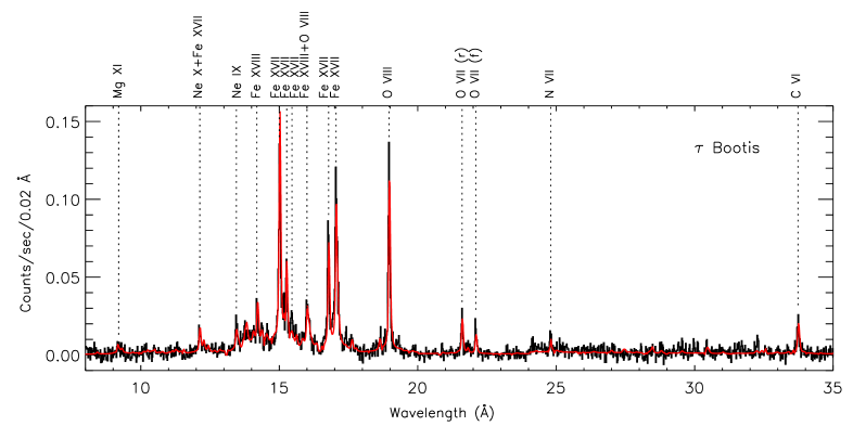
Figure 2: Summed RGS1 and RGS2 spectra of $\tau$ Bootis (histogram) with the synthetic model spectrum derived from the analysis results obtained with Method 1. Labels identify some of the strongest lines.

4.1 RGS data analysis

The background-subtracted RGS1 and RGS2 spectra of $\tau$ Boo contain $\sim 4000$ and $\sim 5100$ net counts, respectively (Fig. 2).

The analysis of X-ray emission line spectra is notoriously difficult, and the measurement of element abundances can be affected by systematic uncertainties that are difficult to quantify because of the assumed plasma emissivity model, the identification and measurement of relevant lines, and the algorithm adopted for the emission measure analysis (Maggio, 2007). For this reason, we employed two different approaches for the analysis of the XMM-Newton grating spectra of $\tau$ Boo, carried out in a completely independent manner.

4.1.1 Method 1

The first approach is the one discussed in detail in Scelsi et al. (2004) together with a study of its accuracy; here we limit ourselves to report the main points of this iterative method.

We employed the software package PINTofALE V2.0 (Kashyap & Drake, 2000) and, in part, also XSPEC, and used the Astrophysical Plasma Emission Database (APED/ATOMDB V1.3, Smith et al., 2001), which includes the Mazzotta et al. (1998) ionization equilibrium.

Background-subtracted RGS1 and RGS2 spectra were first re-binned by a factor of 2 and then co-added for the identification of the strongest emission lines and the measurement of their fluxes. In the rebinned RGS1+RGS2 spectrum we identified about 40 lines from Fe xvii-xxi, Ne ix-x, O vii-viii, N vii, C vi, and Ni xix-xx ions. After this step the method proceeds in an iterative way.

To measure line fluxes we adopted a Lorentzian line profile and initially assumed the continuum level evaluated from a 3-T model best-fitting the pn spectrum. Indeed, the wide line wings make it impossible to determine the true source continuum below $\sim 17$ Å directly from the RGS data, especially in the $\sim 10-17$ Å range where the spectrum is dominated by many strong overlapping lines. The Mg xi triplet was measured as a single feature by counting the photons within the $9.10-9.40$ Å range in the RGS spectrum rebinned by a factor of 5, and subtracting the assumed continuum contribution in the same wavelength region. We also fixed $N_{\rm H}=3\times 10^{18}$ cm^-2, compatible with the short distance of $\tau$ Boo (15.6 pc). The results are listed in Table LABEL:tab:lines.

To reconstruct the emission measure distribution (EMD, defined as $E\!M(T)=\int_{\Delta T}n_{H}n_{e}dV$ [cm^-3]) and to estimate element abundances, we selected a set of 19 lines among those identified that had reliable flux measurements and theoretical emissivities. Most of them are blended with other lines, so the measured line flux is actually the sum of the contributions of a number of atomic transitions. Accordingly, the ”effective emissivity” of each line blend must be evaluated as the sum of the emissivities of the lines that mostly contribute to that spectral feature. If the blend includes lines from different elements, the effective emissivity needs to be weighted by their relative abundances. Since these abundances are not available at the beginning of the analysis, we initially selected only iron lines not blended with lines of other elements, and the latter are included one at a time in the following stages.

We performed the EMD reconstruction with the Markov-Chain Monte Carlo (MCMC) method by Kashyap & Drake (1998). This method yields a volume emission measure distribution, $EM(T_{k})=dem(T_{k})\,\Delta\log T$, and related statistical uncertainties $\Delta EM(T_{k})$, where $dem(T)=n_{\rm e}^{2}\,{\rm d}V/{\rm d}\log T$ is the differential emission measure of an optically thin plasma and $\Delta\log T=0.1$ is a constant bin size. The method also provides estimates of element abundances scaled by the iron abundance, with their statistical uncertainties. The iron abundance is estimated by computing the emission measure distribution assuming different metallicities and by comparing the synthetic continuum with the observed one at $\lambda>20$ Å in the RGS spectrum, which is a spectral region free of strong overlapping emission lines. Finally, we checked the solution obtained with the MCMC by comparing (i) the line fluxes predicted from our solution with the measured ones and (ii) the whole model spectrum with the observed one (Fig. 2).

The procedure described above is repeated two or three times to check line identifications and to ensure consistency between the continuum level assumed for flux measurements and the continuum predicted by the EMD. Indeed, the continuum is adjusted at each iteration because it may become different from that predicted by the $3-T$ model best-fitting the pn spectrum, which is adopted as the initial guess. This procedure ensures that possible cross-calibration offsets between pn and RGS do not affect the final $EMD$.

The final $EM(T)$ values are reported in Table 3 with the coronal abundances of individual elements. The EMD is also shown in Fig. 3 with the distribution obtained with Method 2.

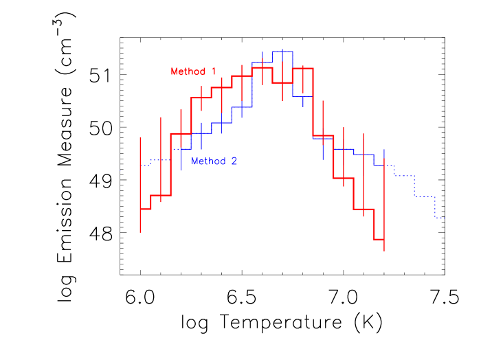
Figure 3: Emission measure distribution of $\tau$ Boo based on the XMM-Newton RGS spectra. The thick (red) histogram was obtained with Method 1 (Scelsi et al., 2004), the thin (blue) histogram with Method 2 (Sanz-Forcada et al., 2003). In the latter, dot-lined bins are more uncertain (no associated error bar).

Table 3: Volume emission measure distribution and coronal abundances of Tau Boo

	RGS
	Method 1	Method 2	EPIC
$\log T$ [K]	$\log EM\,\mathrm{[cm^{-3}]}$
6.0	48.45${}^{1.36}_{0.45}$	49.28	…
6.1	48.70${}^{1.48}_{0.12}$	49.38	…
6.2	49.87${}^{0.46}_{0.26}$	49.58${}^{0.20}_{0.40}$	…
6.3	50.56${}^{0.22}_{0.25}$	49.88${}^{0.20}_{0.30}$	50.94${}^{0.08}_{0.05}$
6.4	50.75${}^{0.19}_{0.48}$	50.08${}^{0.20}_{0.20}$	…
6.5	50.97${}^{0.21}_{0.47}$	50.38${}^{0.40}_{0.20}$	…
6.6	51.13${}^{0.18}_{0.33}$	51.23${}^{0.20}_{0.05}$	51.70${}^{0.02}_{0.02}$
6.7	50.84${}^{0.41}_{0.34}$	51.43${}^{0.05}_{0.20}$	…
6.8	51.11${}^{0.05}_{0.47}$	50.58${}^{0.00}_{0.20}$	…
6.9	49.84${}^{0.66}_{0.18}$	49.78${}^{0.20}_{0.40}$	50.93${}^{0.06}_{0.04}$
7.0	49.03${}^{0.97}_{0.16}$	49.58${}^{0.20}_{0.30}$	…
7.1	48.44${}^{1.44}_{0.13}$	49.48${}^{0.30}_{0.40}$	…
7.2	47.87${}^{1.54}_{0.22}$	49.28${}^{0.30}_{0.30}$	…
Elem.	$A_{\rm c}/A_{\odot}$		$A_{\rm c}/A_{\odot}$
C	0.49${}^{0.08}_{0.15}$	0.55${}^{0.23}_{0.16}$	0.6
N	0.24${}^{0.08}_{0.07}$	0.39${}^{0.27}_{0.16}$	0.4
O	0.22${}^{0.04}_{0.03}$	0.47${}^{0.22}_{0.15}$	0.27${}^{0.02}_{0.01}$
Ne	0.34${}^{0.04}_{0.05}$	0.37${}^{0.13}_{0.10}$	0.31${}^{0.04}_{0.04}$
Mg	0.50${}^{0.08}_{0.10}$	…	0.53${}^{0.06}_{0.04}$
Si	…	…	0.82${}^{0.09}_{0.08}$
S	…	…	= Fe
Ar	…	…	= Fe
Fe	0.50${}^{0.08}_{0.09}$	0.52${}^{0.15}_{0.12}$	0.52${}^{0.01}_{0.01}$
Ni	1.19${}^{0.32}_{0.29}$	2.40${}^{0.91}_{0.66}$	= Fe

4.1.2 Method 2

The second approach for constructing the EMD vs. temperature follows the line-based analysis described in Sanz-Forcada et al. (2003) and references therein. In short, individual line fluxes are measured and those with a signal-to-noise ratio $S/N>$ 3–4 are then compared with the theoretical values obtained from a trial EMD, combined with the same atomic emission model used for Method 1. The comparison of measured and model line fluxes results in an improved EMD that is used again to produce new model line fluxes.

In Method 2 we employed 27 lines. The first iteration is based only on Fe lines, either blended or unblended, assuming solar abundances. The successive iterations are used to calculate the abundances of the different elements, that are required to refine in particular the line predictions for all the blends. Because the lines corresponding to the various elements are formed in different temperature ranges, we take the caution to progressively add lines of elements with formation temperatures that overlap the EMD computed at each iteration.

The method converges in a few iterations, and is therefore self-consistent. This process yields an EMD solution that is not unique, but reliably matches the model fluxes to the observed ones, and it presumably describes the actual amount of plasma at different temperatures in corona.

Finally, error bars are calculated using a Monte Carlo method that seeks the best solution for different line fluxes within their 1–$\sigma$ errors (see Sanz-Forcada et al., 2003, for more details).

In summary, the two methods differ in the choice of the line set employed for the EMD reconstruction, in the algorithm to search for the best EMD solution, and in the evaluation of its confidence range.

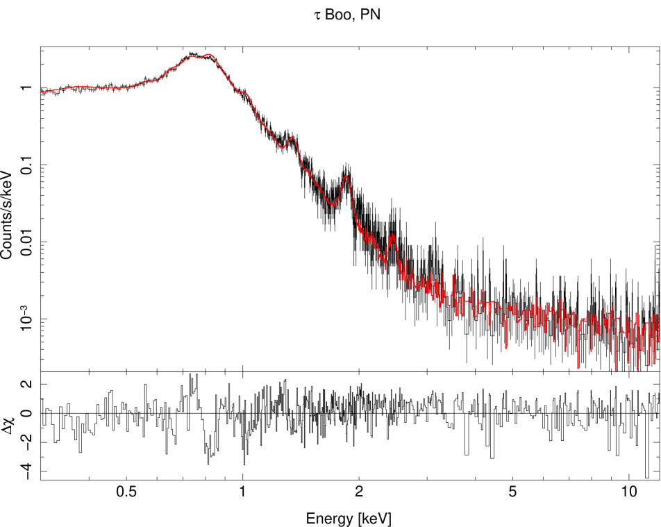
Figure 4: Upper panel: PN observed spectrum (black histogram with error bars)) and best-fit model (in red). Lower panel: residuals in sigma units.

.

4.2 EPIC spectral analysis

Typical EPIC spectra can usually be fitted with thermal models with few (2 – 4) isothermal components. This is an approximation to the actual emission measure distribution of the coronal plasma, which provides a reasonably good quality of the fit to individual CCD-resolution X-ray spectra (MOS or PN); instead, systematic errors and cross-calibration uncertainties make the joint analysis of all the available spectra (EPIC and RGS) cumbersome, and yield best-fit $\chi^{2}$ values formally too high to be statistically acceptable. This is also the case for $\tau$ Boo.

The simplest multi-component thermal model that provides an acceptable fit to the EPIC spectra is a three-temperature model with plasma at 2 MK, 4 MK, and 8 MK and a volume emission measure in the proportions 1:6:1 (see Table 3 and Fig. 4). This model fitting confirms the low interstellar absorption assumed in the analysis of the RGS spectra (Sect. 4.1.1), and yields an independent measure of the abundances of O, Ne, Mg, Si, and Fe. Note that Mg and Si abundances can be effectively constrained by this fitting, because the EPIC spectra clearly show line complexes caused by Mg xi (1.33–1.35 keV), Mg xii (1.47 keV), and Si xiii (1.84–1.86 keV). Abundances of other elements cannot be constrained by the EPIC spectra, and they have been fixed either to the values derived from the analysis of the RGS spectra, or to the iron abundance; in this way, the best-fit model also reproduces sufficiently well the weak spectral feature visible at the expected position of the S xv triplet (2.43–2.46 keV).

5 Discussion

5.1 Abundance depletion in the corona of $\tau$ Boo

The central result of our analysis is illustrated in Fig. 5: the coronal abundances of our target are all systematically lower than the photospheric ones, with the only possible exception of the Ni. In this respect, there is agreement on the abundances derived with any of the methods we employed for all elements but oxygen and nickel, within the statistical uncertainties. The $2\sigma$ difference in the former case can be easily explained by inspection of Fig. 3, where the emission measure derived with Method 1 in the temperature range $\log T=6.3$–6.5 is systematically higher than indicated by Method 2: since much of the O vii and O viii line fluxes are produced in this range, an uncertainty in the emission measure implies a systematic error in the abundance of this element. The case of the Ni abundance is less obvious, but likely because in APED/ATOMDB V1.3 the Ni atomic model is less accurate than for other elements, and the Ni lines are in general relatively faint and hence affected by larger measurement uncertainties.

Regardless of the method, our results show that the coronal iron abundance is about half the solar photospheric value, while the stellar photosphere is twice the same value. The statistical uncertainty on the ratio of the photospheric to coronal iron abundance is very small: $0.24\pm 0.09$ with Method 1, and $0.23\pm 0.06$ with Method 2 (uncertainties computed in quadrature), but an additional (systematic) source of uncertainty on the absolute coronal abundances derived from high-resolution X-ray spectra can be caused by the determination of the continuum emission level. However, the completeness and accuracy of atomic databases for the synthesis of multi-temperature model spectra was significantly improved in the last decade (Brickhouse, 2008), and the results of our RGS data analysis are confirmed by the spectral fitting of the EPIC data as well.

We conclude that our results are sufficiently robust to state that the X-ray emitting plasma of $\tau$ Boo is significantly depleted in metals compared with the photosphere. Although the determination of the absolute iron abundance in the corona may be affected by an uncertainty larger than indicated by our analysis, the pattern of abundances scaled by Fe is well constrained and the available RGS and EPIC spectra exclude a plasma metallicity matching the stellar photospheric composition.

Moreover, we find little if any dependence of the coronal abundances on the first ionization potential (FIP), a result which holds true also considering the coronal vs. photospheric abundance ratios (Fig. 6), rather than values with respect to the solar chemical composition. In this respect, our results would not change after the possible choice of solar element abundances more recent than the Anders & Grevesse (1989) reference scale, which we preferred for consistency with the majority of the previous abundance studies.

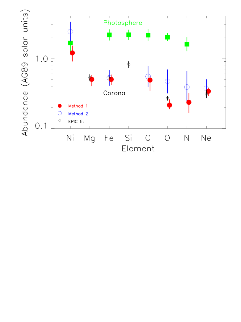
Figure 5: Photospheric and coronal abundances of $\tau$ Boo, sorted by increasing First Ionization Potential. The reference solar abundances are by Anders & Grevesse (1989).

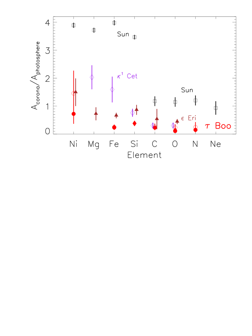
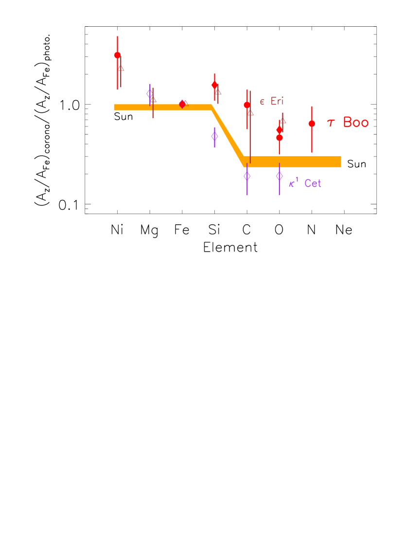
Figure 6: Upper: Coronal to photospheric abundance ratios for the Sun (black squares), $\tau$ Boo (red circles and filled diamonds), and two other intermediate-activity stars (magenta empty diamonds for $\kappa^{1}$ Cet and brown triangles for $\epsilon$ Eri). Elements are sorted as in Fig. 5. Lower: Same plot but with all values divided by the Fe abundance in a logarithmic scale. The FIP bias in the solar corona is indicated by the shaded (orange) strip, and for $\tau$ Boo the abundances obtained with Method 2 are not shown for clarity.

5.2 $\tau$ Boo: a medium-activity coronal source

In order to put the coronal abundances of $\tau$ Boo in context, Fig. 7 shows a comparison of its EMD distribution vs. temperature (Method 1) with those of other four G-K stars: the Sun (G2V, Peres et al., 2000), $κ^1$ Ceti (G5V, Telleschi et al., 2005), $ϵ$ Eri (K2V, Sanz-Forcada et al., 2004), and HD 283572 (G2IV, Scelsi et al., 2005).

The relative amount of plasma at different temperatures is a way to judge the level of stellar magnetic activity, and it carries more information than a simple comparison of broad-band X-ray luminosities. Among the stars we selected, the Sun is clearly the one with the lowest average temperature, with an EMD that peaks just below 2 MK. At the other extreme, HD 283572 is a young weak-lined T Tauri star in the Taurus-Auriga region with a much hotter and X-ray bright corona at 10–20 MK. The other three stars were selected instead for the similarity of their EMD with that of $\tau$ Boo. $\epsilon$ Eri is also known to host a Jovian-mass planet ($m\sin i\approx 1.6\,{\rm M_{\rm J}}$) at a distance of 3.4 AU, while $\kappa^{1}$ Cet is a putative single star.

In passing we note that $\tau$ Boo also has a stellar companion, GJ 527 B, with spectral type M2 (V=11.1) (Patience et al., 2002). We evaluated the possible contamination to the observed X-ray flux by deriving the B-V color and the bolometric correction from the spectral type and adopting the transformations by Flower (1996), and thus obtaining for the bolometric luminosity $\log L_{\rm bol}=30.96\leavevmode\nobreak\ {\rm ergs^{-1}}$. Assuming, conservatively, that the GJ 527 B X-ray emission is at the saturation level, we get $L_{\rm x}=10^{-3}L_{\rm bol}\la 10^{28}\leavevmode\nobreak\ {\rm ergs^{-1}}$, which is about a factor 10 lower than the X-ray luminosity of $\tau$ Boo ($\log L_{\rm x}=28.94\leavevmode\nobreak\ {\rm ergs^{-1}}$, in the 0.1–2.4 keV band). We conclude that the contamination from this unresolved companion is negligible.

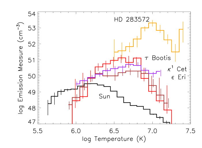
Figure 7: Emission measure distribution of $\tau$ Boo (Method 1) compared with those of other G- or K-type stars with different activity levels, including the quiescent solar corona (see text for references).

We took the photospheric abundances for $\epsilon$ Eri from Gonzalez & Laws (2007), the same source as for $\tau$ Boo, while for $\kappa^{1}$ Cet we adopted the photospheric composition by Allende Prieto et al. (2004), which was determined in a strictly differential way with respect to the Sun. The coronal abundances of the same two stars were derived by Sanz-Forcada et al. (2004) and by Telleschi et al. (2005) respectively, with an analysis of XMM-Newton data similar to ours. We then computed the coronal/photospheric abundance ratios of all the solar-type dwarfs in our sample, excluding HD 283572 because of its peculiar evolutionary phase and extreme activity level.

The pattern of abundance ratios vs. FIP (Fig. 6) appears very similar for $\tau$ Boo and $\epsilon$ Eri, and significantly different from the solar case, which is characterized by the well-known FIP effect (Feldman & Laming, 2000). Finally, $\kappa^{1}$ Cet displays an overabundance of low-FIP elements (Mg and Fe) in the corona, although with relatively large uncertainties on the abundance ratios, but high-FIP elements (C and O) are underabundant with respect to the photospheric composition, which is not the case in the solar corona. In the right panel of Fig. 6 we also show a comparison of all the coronal/photospheric abundance ratios scaled by the iron abundances, because relative abundances are considered more robust than absolute abundances. This plot clearly shows that in $\tau$ Boo and $\epsilon$ Eri there is a smaller (if any) dependence of the abundance ratios on FIP than in the solar case.

The above comparison suggests that the outer atmospheres of some intermediate activity stars, like $\tau$ Boo and $\epsilon$ Eri are not affected by a FIP-dependent chemical stratification as pronounced as in the solar case. A closer look at the left panel in Fig. 6 shows however that only for $\tau$ Boo the coronal abundances are significantly and uniformly lower than the photospheric ones (with the possible exception of Ni).

Common understanding is that the abundance patterns in low- and high-activity stars are different, with low-activity stars showing an overabundance of low-FIP elements in the corona (positive FIP effect), while high-activity stars are characterized by the reverse behavior (inverse FIP effect) (Audard et al., 2003). Following this activity-dependence scenario (see e.g. Güdel & Nazé, 2009), an abundance ratio Ne/Fe $\sim 0.25$ (with respect to the photospheric value) is expected for Sun-like stars, while Ne/Fe $\sim 5$–10 in very active stars. An intermediate activity star with an EMD similar to those of $\tau$ Boo, $\epsilon$ Eri, and $\kappa^{1}$ Cet, should display Ne/Fe $\sim 1$.

However, this scenario was constructed assuming stellar photospheric abundances similar to the solar ones – a common practice for many years – which has recently been challenged by studies where coronal abundances are compared to accurate measurements of stellar photospheric abundances: in most cases, this properly consistent comparison has shown little if any significant difference between photospheric and coronal compositions (Sanz-Forcada et al., 2004; Maggio et al., 2007; Sanz-Forcada et al., 2009).

The novel result of our work is that $\tau$ Boo does not show any evident FIP bias, but that on the other hand the coronal abundances are all significantly lower with respect to the photospheric ones by factors of 3 to 9 (taking into account the uncertainties, and with the exception of Ni). Hence, the case of $\tau$ Boo demonstrates that coronal and photospheric abundances may differ in a peculiar FIP-independent way, which was never reported this clearly before the present study.

This result represents a new challenge for theoretical models that try to explain element fractionation in stellar outer atmospheres. In spite of many attempts in the past, the only model that is capable of producing either a positive or an inverse FIP effect is the one proposed by Laming (2004, 2009). In this model charged ions are subject to a ponderomotive force caused by Alfvén waves propagating through the chromosphere, which may originate either in the corona or in the convection zone. Depending on whether the waves are reflected or not at the base of coronal magnetic loops, the ponderomotive force can point upward or downward, producing opposite effects. Low-FIP elements are primarily affected because they are nearly fully ionized in the upper chromosphere, whereas high-FIP elements are partially neutral. In any case, the element fractionation is expected to show a FIP-dependence, which is apparently lacking in the outer atmosphere of $\tau$ Boo.

6 Summary and conclusions

We performed a detailed comparison of the photospheric and coronal abundances of the planet-hosting star $\tau$ Boo, making use of the best optical and X-ray spectroscopic data available to date. We analyzed high-resolution spectra obtained with the reflection gratings (RGS) on-board the XMM-Newton satellite, and also medium-resolution (EPIC) spectra with much higher photon counting statistics. The emission measure distribution vs. temperature and element abundances of the coronal plasma were derived with two independent methods from the RGS data, and confirmed with the analysis of the EPIC spectra.

In spite of some $2\sigma$ difference in the EMDs derived with the two methods, a robust and consistent result is that the coronal abundances of $\tau$ Boo are significantly lower than the photospheric ones, by about a factor 4, on average. The largest uncertainty is for the oxygen abundance, whose underabundance factor is in the range 4–9. We do not see any way to bring coronal and photospheric abundances into agreement, unless the coronal Fe abundance is 4 times larger than the present best estimate ($\approx 0.5$ the solar one), but such a systematic error is very unlikely with data of the present quality and with the state-of-the-art analysis methods we employed.

Assuming solar abundances as reference, the pattern of coronal abundances vs. FIP is nearly flat, and this behavior is also confirmed when the actual $\tau$ Boo photospheric abundances are considered. No important FIP-dependent element stratification mechanism appears to be at work in the outer atmosphere of $\tau$ Boo, but the metallicity in the corona is very different from the photospheric one. It is unclear at the moment whether this is a peculiarity of metal-rich stars.

From a complementary point of view, while the coronal characteristics of $\tau$ Boo including absolute abundances are similar to other intermediate-activity stars, its photospheric abundances are recognized to be quite large for Galactic old-disk standards and linked to its being a star hosting a close-in giant planet. Our results challenge the present understanding of chemical stratification effects in the atmospheres of solar-type stars, and the possible role of stellar activity in the underlying physical mechanism.