The EXOTIME targets HS 0702+6043 and HS 0444+0458

Abstract

Pulsations in subdwarf B (sdB) stars are an important tool to constrain the evolutionary status of these evolved objects. Interestingly, the same data used for this asteroseismological approach can also be used to search for substellar companions around these objects by analyzing the timing of the pulsations by means of a so-called O–C diagram. Substellar objects around sdB stars are important for two different reasons: they are suspected to be able to influence the evolution of their host-star and they are an ideal test case to examine the properties of exoplanets which have survived the red giant expansion of their host stars.

1 Introduction

Hot subdwarf B (sdB) stars are evolved objects with canonical masses close to half a Solar mass. They are burning helium in their core and populate the so-called extreme horizontal branch (EHB). During their evolution on the Red Giant branch, the progenitors must suffer an extreme mass loss, such that at the time of the helium flash there is only a very thin hydrogen envelope left. The thin envelope is inert and prevents the sdB from shell burning and therefore from an evolution towards the AGB and PN phases. Instead, these objects are believed to directly evolve to the White Dwarf cooling sequence (see Fig. 1).

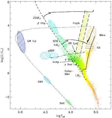
Figure 1: Pulsational Hertzsprung-Russell diagram showing the location of the variable subdwarf B stars (sdBV). Modified version from http://astro.phys.au.dk/HELAS/puls_HR.

There is also the possibility that sdB stars show pulsations driven by a $\kappa$ mechanism related to an opacity bump caused by iron group elements (Charpinet et al., 1997). Two different types of modes can appear: short period pressure (p-) modes or long period gravity (g-) modes. For both groups, the rapidly pulsating sdBV_r and the slowly pulsating sdBV_s stars, the amplitudes can be as low as only some mmag. There also exist a few hybrid objects (sdBV_rs) belonging to both groups (Schuh et al., 2006; Lutz et al., 2009).

Examining the pulsations of sdB stars provides the observational input for asteroseismological modeling, in order to characterize the internal structure. Furthermore, a measured change in the period, $\dot{P}$, can additionally constraint asteroseismological models and give hints on mode identification. Measuring $\dot{P}$, and therefore determining the evolutionary timescale, is one of our goals.

The search for exoplanets around sdB stars is another goal of our project: more than 490 exoplanets are known to date. Due to the applicability of the common detection methods as well as the specific goal to find an Earth-analogon in a solar-system-like exo-system, most of the exoplanet surveys are focused on solar-like stars on the Main Sequence. However, little is known about the late stages of exoplanetary system evolution, in particular the fate of exoplanets during and after the Red Giant expansion of the host star. The number of exoplanets around Giant and Subgiant stars is increasing, but still low compared to the Main Sequence hosts. The same is true for White Dwarfs and for hot subdwarfs. The latter are the type of star that we aim to consider here. Finding exoplanets around sdB stars might be immediate proof that exoplanets would be able to survive the host star expansion or even a common envelope phase.

The formation of sdB stars is not very well understood: the binary sdB population can quite well be explained by the current binary formation channels including common envelope evolution and stable and unstable RLOF (Han et al., 2002), however there are issues to explain apparently single sdB stars. One of the more promising scenarios for single sdB formation is given by Soker (1998), who examines the possibility of enhanced mass loss of the sdB progenitor during the Red Giant phase induced by substellar companions. Therefore, finding substellar objects around single sdB stars would directly support this hypothesis.

We aim to apply a timing method (O–C analysis, observed minus calculated) to search for substellar companions around pulsating sdB stars. At the same time, with the same data, we are able to derive the evolutionary timescales for these objects. Different shapes of an O–C diagram can be interpreted as follows: a parabolic trend indicates a linear change in the pulsation period which is under consideration. From this quadratic O–C, one can calculate a value $\dot{P}$, i.e. the change of the pulsation period with time. This $\dot{P}$ can then be translated to an evolutionary timescale $T_{evol}$ of the pulsating sdB star via

$$T_{evol}=P/\dot{P}.$$ (1)

In addition, finding sinusoidal residuals can most plausibly be explained by an orbital reflex motion of the pulsating star, where the timing signals used to construct the O–C diagram in our case are the times of maximum intensity. Concerning sdB stars, the object HS 2201+2610 is the only object where an O–C analysis has been published yet. Silvotti et al. (2007) find an evolutionary timescale of 7.6 Myr and also the signal of an exoplanetary companion with a minimum mass of 3.2 times Jupiter’s mass in an orbit of 1170 days. This exoplanet is the first one having been detected around a sdB star. If this object formed as a first generation planet at the same time as the host star, it would be direct proof that the substellar object survived the Red Giant expansion of its host star. Triggered by this discovery, we set up the EXOTIME program (see next section). Fourier transforms of our full data sets of HS 0444+0458 (left) and HS 0702+6043 (right). The total time base is 19 months and 28 months, respectively. See more details in Table 1.

2 Observations

The search for exoplanets around pulsating sdB stars is an ongoing program: long-term photometric observations are organized in the EXOTIME program (EXOplanet search with the TIming MEthod, lead by R. Silvotti & S. Schuh). A recent review on the status is given by Schuh et al. (2010). A basic factor for a pulsating sdB star to be examined for substellar companions with the timing method is the characteristic of its periodogram. A suitable target shows not too many frequencies, moderately large and stable amplitudes and a suitable magnitude. Most importantly, the pulsations must adhere to phase coherence to a sufficient degree. The targets considered here have been tested to fulfill these conditions. HS 0702+6043 (Fig. 1) is a hybrid sdB pulsator (sdBV_rs) showing a main pulsation period of 382s with an amplitude around 27 mmag (Dreizler et al., 2002; Lutz et al., 2008). HS 0444+0458 (Fig. 1) is a p-mode pulsator (sdBV_r) with a main pulsation period of 137s with an amplitude of 7 mmag (Østensen et al., 2001).

To derive a single point for the O–C diagrams of our selected targets, observations during on average at least three to four consecutive nights with at least two to three hours per target per night are required. The minimum time base of three nights for each block is needed to resolve the pulsational frequencies. At least three hours per night are needed for each object to sample enough pulsational cycles. Since we look at low-amplitude, short-period p-modes (some mmag on a timescale of about five minutes or less) we require both a short sampling time of less than about 30s and very high signal to noise during these short exposures to detect the low amplitudes. EXOTIME conducts regular long-term time-series photometry using several small- to medium-class telescopes. A current list of our photometric data archive for the targets HS 0444+0458 and HS 0702+6043 is given in Table 1.

Site and mirror size	HS 0444+0458 Aug 2008 – Feb 2010	HS 0702+6043 Nov 2007 – Feb 2010
Mt. Bigelow 1.56m		424 h
Calar Alto 2.20m	32 h	116 h
MONET/N 1.20m	16 h	98 h
Tue 0.80m		62 h
Goe 0.50m		53 h
LOAO 1.00m	16 h	43 h
TNG 3.60m	7 h
Asiago 1.82m		20 h
Loiano 1.52m		14 h
Konkoly 1.00m		14 h
St. Bok 2.20m		12 h
Moletai 1.60m		8 h
NOT 2.56m		1 h
total	71 h	865 h

Table 1: Photometric data for HS 0444+0458 and HS 0702+6043

3 Data Reduction

After extracting relative light curves in a standard aperture photometry procedure, detrending and normalization, it is also absolutely crucial to do the time correction for Earth’s motion in the Solar System properly (the reference point is the barycenter of the Solar System). In addition, one needs to be aware of leap seconds. At this stage, there are the relative normalized light curves given in barycentrically corrected time (BJD) versus relative intensity.

Since data from different telescope sites are of different quality, we apply a weighting scheme to the light curves. Point weights $w$ are assigned to each light curve data point according to $w=\frac{1}{\sigma^{2}}$, with $\sigma$ being the standard deviation calculated on a subset of $n$ data points, centered on each time stamp, after having subtracted the pulsation frequencies. This can be described as sort of a ”moving standard deviation”. $n$ is an integer, usually corresponding to the number of data points within two or three pulsational cycles. Gaps are also taken into account. We use a routine provided by one of us (RS).

4 Timing method and O–C diagram

The O–C analysis as a particular application of the timing method is an approach to measure the phase variations of a periodic function. In our case, these periodic functions are the pulsations of the sdB star leading to periodic intensity variations. Other applications include the timing of Pulsar signals and the timing of eclipses in eclipsing binary systems. In all cases the periodic signal is used as a clock and one wants to examine the behaviour of this clock as a function of time. To do so, it is reasonable to compare the calculated (”C”-part of the O–C diagram) light curve solution of the whole data set with the actually observed (”O”-part of the O–C diagram) light curve solutions of temporal subsets of the whole data set.

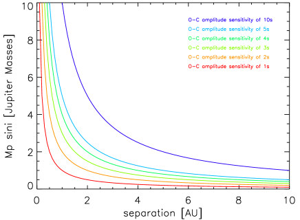
Figure 2: Sensitivity of the timing method applied to pulsating sdB stars. We assume different amplitude sensitivities ranging from 10s (uppermost line) to 1s (lowermost line). The justification of the assumed amplitude sensitivities mainly depends on the total time base of observational data being available.

In a first step, a light curve solution is determined for the full light curve. Since sdB stars are multi-mode pulsators, the solution will consist of a frequency, amplitude and phase for each pulsation considered. The frequency solution of this full light curve (the ”C” part) is then kept fixed and each seasonal light curve is being fitted with that fixed frequency, while determining the amplitudes and phases of the seasonal light curves (the ”O” parts). It is sometimes also be possible to keep both the frequency and the amplitude of the full light curve fixed. For each seasonal light curve the phase difference to the full light curve can now be determined. These phase differences are translated to time differences, which, plotted as a function of time, yield an O–C diagram.

Assuming a reflex motion of the sdB caused by a substellar companion (translating into a sinusoidal component in the O–C diagram), one can find a relation between the O–C amplitude $\tau$ and the orbital separation $a$. Given the assumptions of a two body case, a circular orbit, a canonical sdB mass of 0.5 solar masses, $M_{p}\ll M_{\star}$, and scaling to Solar System units, one obtains

$$M_{p}\cdot\sin{i}=\tau\cdot\frac{1}{a},$$ (2)

with the companion’s mass $M_{p}[M_{Jup}]$, the inclination $i$ and orbital separation $a[AU]$ . The O–C amplitude $\tau[s]$ is a quantity measured in the O–C diagram, such that assuming different given amplitude sensitivities, one can plot the minimum detectable planetary mass versus the orbital separation. This simple estimation has been done for different amplitude sensitivities in Fig. 2. As can be seen, the timing method applied to pulsating sdB stars is more sensitive towards larger separations.

O–C diagram (left) for the main frequency f1 of HS 0444+0458. The symbols with error bars are seasonal data currently available. The dashed line is a parabolic component yielding a $\dot{P}$ of $6.00\cdot 10^{-12}$ d/d or an evolutionary timescale of 0.72 Myr. We proceed to specifically look for sinusoidal residuals, which might hint at a reflex motion of a possible companion. The solid line in the right panel shows a periodogram of the residuals based on the current data with a peak around 160 days at a significance of only 1$\sigma$. Boldly assuming an orbit of 160 days, we calculate the expected signature in the O–C (solid line in the left panel). The triangles refer to future observations. The predicted effect of the increased time baseline due to the future observations on the significance in the residual periodogram is shown as the dashed line in the right panel. If upcoming data support our current model, the significance in the residual periodogram would rise above 2$\sigma$, strengthening the hypothesis of a substellar companion candidate (not currently claimed as real).

Same as Fig. 2, but for the main frequency f1 of HS 0702+6043. The parabolic component yields a $\dot{P}$ of $6.81\cdot 10^{-12}$ d/d, translating to an evolutionary timescale of 1.69 Myr. The residuals reveal no significant orbital signal so far.

Same as Fig. 2, but for the second frequency f2 of HS 0702+6043. The parabolic component yields a $\dot{P}$ of $8.39\cdot 10^{-12}$ d/d, translating to an evolutionary timescale of 1.45 Myr. The significant peak close to 3$\sigma$ in the residual periodogram mimics a possible companion in a 80 days orbit, but is most probably due to a beating of close unresolved frequencies. These two close frequencies have an amplitude ratio close to 2:1 and can only be resolved in the full data set, but not in the shorter seasonal subsets.

5 Results

To get independent results, we conducted the O–C analysis not only for the strongest frequencies (f1) in HS 0444+0458 and HS 0702+6043, but also for the second strongest ones (f2). Table 2 gives a summary of the frequencies used for the analysis and our results for $\dot{P}$ and the evolutionary timescales. The O–C diagram of the strongest frequency f1 in HS 0444+0458 is shown in Fig. 2. Although we find much more pulsations in the FT of the full data set of HS 0702+6043, these are too weak to be included in the detailed O–C analysis. O–C diagrams for f1 and f2 of HS 0702+6043 are visualized in Figs. 2 and 2.

	Label	Frequency [1/d]	Amplitude [mma]	$\dot{P}$ [d/d]	$T_{evol}$ [Myr]
HS 0444+0458	f1	631.735086	7.13	$6.00\cdot 10^{-12}$	0.72
	f2	509.977714	2.53	$5.27\cdot 10^{-12}$	1.02
HS 0702+6043	f1	237.941086	27.51	$6.81\cdot 10^{-12}$	1.69
	f2	225.158793	5.60	$8.39\cdot 10^{-12}$	1.45

Table 2: Frequencies used for the O-C analysis and evolutionary timescales of the corresponding pulsations

6 Discussion

One goal of the EXOTIME program is to determine the evolutionary timescales of pulsating sdB stars. Here, we considered two particular objects and analyzed the currently available photometry covering baselines of 19 and 28 months. The $T_{evol}$ values found for both modes f1 and f2 in HS 0702+6043 and HS 0444+0458 are compatible with current models (Charpinet et al., 2002). Our results are also compatible with those found for HS 2201+2610 (V 391 Peg): Silvotti et al. (2007) find a $\dot{P}$ of $1.46\cdot 10^{-12}$ and $2.05\cdot 10^{-12}$ for the two strongest frequencies, corresponding to evolutionary timescales of 7.6 Myr and 5.5 Myr, respectively.

The second part of the EXOTIME program, examining the targets for substellar companions, does not come to a conclusion yet. The significance of any periodic signals in the residual periodograms is too low, but we make testable predictions for HS 0444+0458. The particular strength of the timing method, its ability to uncover planets in wide orbits, at the same time means that long timescales are involved: for detecting a planet in a x-year orbit one obviously needs a time base of more than x years to uncover it. The timing method is therefore very consuming in terms of observing time if applied in a way to really play its strength. Provided that we will regularly gather more data, we expect to give a detailed statement on the possibility of the presence of substellar companions within the next year.

References

- Charpinet et al. (1997) S. Charpinet, G. Fontaine, P. Brassard, P. Chayer, F. J. Rogers, C. A. Iglesias, and B. Dorman, ApJ 483, L123–L126 (1997).
- Charpinet et al. (2002) S. Charpinet, G. Fontaine, P. Brassard, and B. Dorman, ApJS 140, 469–561 (2002).
- Dreizler et al. (2002) S. Dreizler, S. L. Schuh, J. L. Deetjen, H. Edelmann, and U. Heber, A&A 386, 249–255 (2002).
- Han et al. (2002) Z. Han, P. Podsiadlowski, P. F. L. Maxted, T. R. Marsh, and N. Ivanova, MNRAS 336, 449–466 (2002).
- Lutz et al. (2009) R. Lutz, S. Schuh, R. Silvotti, S. Bernabei, S. Dreizler, T. Stahn, and S. D. Hügelmeyer, A&A 496, 469–473 (2009).
- Lutz et al. (2008) R. Lutz, S. Schuh, R. Silvotti, S. Dreizler, E. M. Green, G. Fontaine, T. Stahn, S. D. Hügelmeyer, and T. Husser, “Light Curve Analysis of the Hybrid SdB Pulsators HS 0702+6043 and HS 2201+2610,” in Hot Subdwarf Stars and Related Objects, edited by U. Heber, C. S. Jeffery, & R. Napiwotzki, 2008, vol. 392 of Astronomical Society of the Pacific Conference Series, pp. 339–342.
- Østensen et al. (2001) R. Østensen, U. Heber, R. Silvotti, J. Solheim, S. Dreizler, and H. Edelmann, A&A 378, 466–476 (2001).
- Schuh et al. (2006) S. Schuh, J. Huber, S. Dreizler, U. Heber, S. J. O’Toole, E. M. Green, and G. Fontaine, A&A 445, L31–L34 (2006).
- Schuh et al. (2010) S. Schuh, R. Silvotti, R. Lutz, B. Loeptien, E. M. Green, R. H. Østensen, S. Leccia, S. Kim, G. Fontaine, S. Charpinet, M. Francœur, S. Randall, C. Rodríguez-López, V. van Grootel, A. P. Odell, M. Paparó, Z. Bognár, P. Pápics, T. Nagel, B. Beeck, M. Hundertmark, T. Stahn, S. Dreizler, F. V. Hessman, M. Dall’Ora, D. Mancini, F. Cortecchia, S. Benatti, R. Claudi, and R. Janulis, Ap&SS p. 130 (2010).
- Silvotti et al. (2007) R. Silvotti, S. Schuh, R. Janulis, J. Solheim, S. Bernabei, R. Østensen, T. D. Oswalt, I. Bruni, R. Gualandi, A. Bonanno, G. Vauclair, M. Reed, C. Chen, E. Leibowitz, M. Paparo, A. Baran, S. Charpinet, N. Dolez, S. Kawaler, D. Kurtz, P. Moskalik, R. Riddle, and S. Zola, Nature 449, 189–191 (2007).
- Soker (1998) N. Soker, AJ 116, 1308–1313 (1998).