About the relative importance of compressional heating and current dissipation for the formation of coronal X-ray Bright Points

Abstract

Context. The solar corona is heated to high temperatures of the order of $10^{6}K$. The coronal energy budget and specifically possible mechanisms of coronal heating (wave, DC-electric fields, ..) are poorly understood. This is particularly true as far as the formation of X-ray bright points (BPs) is concerned.

Aims. Investigation of the energy budget with emphasis on the relative role and contribution of adiabatic compression versus current dissipation to the formation of coronal BPs.

Methods. Three-dimensional resistive MHD simulation starts with the extrapolation of the observed magnetic field from SOHO/MDI magnetograms, which are associated with a BP observed on 19 December 2006 by Hinode. The initial radially non-uniform plasma density and temperature distribution is in accordance with an equilibrium model of chromosphere and corona. The plasma motion is included in the model as a source of energy for coronal heating.

Results. Investigation of the energy conversion due to Lorentz force, pressure gradient force and Ohmic current dissipation for this bright point shows the minor effect of Joule heating in comparison to the work done by pressure gradient force in increasing the thermal energy by adiabatic compression. Especially at the time when the temperature enhancement above the bright point starts to form, compressional effects are quite dominant over the direct Joule heating.

Conclusions. Choosing non-realistic high resistivity in compressible MHD models for simulation of solar corona can lead to unphysical consequences for the energy balance analysis, especially when local thermal energy enhancements are being considered.

1 Introduction

The mechanisms of coronal heating are not well understood. A particular object for studying heating processes are coronal bright points (further abbreviated BPs). Due to the increasing accuracy of observations our knowledge about BP has greatly advanced from the time of their discovery in soft X-ray images Vaiana et al. (1970). According to X-ray and EUV observations the linear size of BPs is on average about 30-40 arcsec with, typically, an embedded bright core of about 5-10 arcsec Madjarska et al. (2003). The average lifetime of X-ray BPs is about 8 hours Golub et al. (1974) and 20 hours for EUV BPs Zhang et al. (2001). For a long time it has been known that BPs are associated with small bipolar magnetic features in the photosphere Krieger et al. (1971); Brown et al. (2001). About one third of BPs lie over emerging regions of magnetic flux, while the rest of them lie above moving magnetic features. This was a base for the ”cancelling magnetic feature” (CMF) model Priest et al. (1994). Lifetime and energy release of BPs are known to be closely related to the different phases of the motion of this photospheric magnetic feature Brown et al. (2001). First theories were mainly addressing the topology of the magnetic field below BPs by e.g., Parnell et al. (1994); Longcope, (1998). Using higher resolution and cadence observations of BP’s intensity and taking into account a more comprehensive patterns of motion in particular in regions with highly divergent magnetic field, (Brown et al., 2001) could associate different patterns of motion of the solar photospheric magnetic features to different stages of a BP evolution. The plasma motion in the regions of strong magnetic field was first included by Büchner (2004a,b) in their three-dimensional numerical resistive MHD model using their 3D numerical simulation model, LINMOD3d. The latter considers dissipation of currents generated by plasma motion in photosphere on time scales longer than an Alfvén time as a one of the heating processes in the solar corona Parker, (1972). In their model they took into account current dissipation due to anomalous resistivity (Büchner & Elkina, 2005, 2006) that causes Joule heating. Since LINMOD3d considers the compressibility of the plasma, the resulting heating could be due also to compressional effects. Later on two-dimensional MHD simulation studies were carried out by von Rekowski B. et al. (2006a, b); von Rekowski et al. (2008). These authors used an analytical initial equilibrium and imposed a magnetic flux footpoint motion to model coronal bright point heating as being due to canceling magnetic features. To obtain the desired heating rate they used an enhanced resistivity for which the values were above the theoretically justifiable resistivity. This raises the general question of the energy budget and energy conversion in solar flux tubes. Even with low resistivity, current simulations are unable to resolve the diffusion regions of reconnection and thus overestimate Joule heating. It is also unresolved how much heating is caused by pressure gradient forces.

To clarify this question we continued the work of Büchner et al. (2004a, b, c); Büchner (2006, 2007); Santos & Büchner (2007); Santos et al. (2008). These authors demonstrated the formation of localized current sheets in and above the transition region at the position of a EUV BPs as a result of photospheric plasma motion. This study is extending their results through a systematic study of the energy conversion and budget in magnetic flux tubes. The investigation uses the 3D simulation model LINMOD3d to simulate the solar atmosphere in the region of an X-ray BP observed by the Hinode spacecraft on 19 December 2006 between 22.17 UT and 22.22 UT.

In section 2 we briefly review the main features of the numerical simulation model LINMOD3d. In section 3 we describe the specific simulation setup used in our study and section 4 provides some simulation results for the chosen BP data. In section 5 we present results of energy budget analysis by investigating the role of different forces and in section 6 we summarize and discuss our results.

2 Simulation model

Our simulation model uses the approach of the LINMOD3d code (Büchner et al., 2004a, b, c). This means that the initial magnetic field is obtained by extrapolating the observed photospheric line-of sight (LOS) magnetic fields. The initial plasma distribution is non-uniform containing a dense and cool chromosphere as well as the transition to a rarefied and hot corona. The photospheric driving is switched on by coupling the chromospheric plasma with a moving background neutral gas. Some details of our code have been given briefly in the following subsection.

2.1 Equations

In our study we solve the following set of MHD equations:

$$\frac{\partial\rho}{\partial t} =-\@vec{\nabla}\cdot\rho\@vec{u}$$ (1)

$$\frac{\partial\rho\@vec{u}}{\partial t} =-\@vec{\nabla}\cdot\rho\@vec{u}\@vec{u}-\@vec{\nabla}p+\@vec{j}\times\@vec{B}-\nu\rho(\@vec{u}-\@vec{u}_{0})$$ (2)

$$\frac{\partial\@vec{B}}{\partial t} =\@vec{\nabla}\times(\@vec{u}\times\@vec{B}-\eta\@vec{j})$$ (3)

$$\frac{\partial p}{\partial t} =-\@vec{\nabla}\cdot p\@vec{u}-(\gamma-1)p\@vec{\nabla}\cdot\@vec{u}+(\gamma-1)\eta j^{2}$$ (4)

where $\rho$ and $\@vec{u}$ are plasma density and velocity, $\@vec{B}$ is the magnetic field and P is the thermal pressure. A plasma-neutral gas coupling in photosphere and chromosphere is included through the collision term in the momentum equation, where $\@vec{u}_{0}$ denotes the neutral gas velocity. The neutral gas serves as a frictional background to communication photospheric footpoint motion to the plasma and magnetic field through frictional interaction. It also leads to a reflection of coronal Alfvén waves back to the corona from the transition region, so that the influence of coronal Alfvén waves can be neglected at the photospheric boundary. In order to set the plasma in motion a number of incompressible flow eddies is used according to observed horizontal drifts in the photosphere $\nabla\cdot\textbf{u}_{0}=0$ is imposed via the neutral gas, where $\textbf{u}_{0}$ is dependent in x and y. It is constant along z and derived from a potential using $\textbf{u}_{0}=\nabla\times(U\textbf{e}_{z})$, with

$$U=u_{00}/\cosh\left(\frac{x-y+c_{0}}{L_{0}}\right)/\cosh\left(\frac{x+y+c_{1}}{L_{1}}\right)$$ (5)

Note that the contour lines of this function are streamlines of the flow. The magnitudes of velocity scale with $u_{00}/L_{0}$ and $u_{00}/L_{1}$, chosen in accordance with the observed plasma motion in the photosphere. In our simulation we approximated the observed motion by three vortices with amplitudes of the velocity $u_{00}$ equal to 5.5, 5 and 2 $km/s$, respectively. The values of $c_{0}$, $L_{0}$, $c_{1}$ and $L_{1}$ are 9, 6, 51 and 6 Mm for the first vortex 5, 6, 28 and 6 Mm for the second and 19, 7, 38 and 7 Mm for the third vortex. The height-dependent collision frequency $\nu$ is chosen to be sufficiently large only below the transition region. This way the plasma is forced to move, dragged by the neutral gas, in the model chromosphere but not above the transition region. This way the horizontal motion generates a Poynting flux into the corona. On the other hand the collision frequency is chosen in a way that coronal Alfvén waves are properly reflected while wave perturbations in the chromosphere are heavily damped by the frictional interaction with the neutral background. Our choice of equations means that in this study we do not consider energy losses due to radiation and heat conduction and we also excluded the action of the solar gravitation in this study. The system of equations is closed by Ohm’s and Ampère’s laws and the temperature is defined via the ideal gas law for a fully ionized plasma:

$$\@vec{E} =-\@vec{u}\times\@vec{B}+\eta\@vec{j}$$ (6)

$$\@vec{\nabla}\times\@vec{B} =\mu_{0}\@vec{j}$$ (7)

$$p =2n\kappa_{B}T$$ (8)

The value of the resistivity $\eta$ is varied in accordance with three models described in subsection 2.3. The MHD equations are discretized by means of a second order weakly dissipative Leapfrog scheme. Due to stability reasons the induction equation is discretized using Dufort-Frankel scheme, Potter (1973).

2.2 Simulation box and normalization

The lower boundary of the simulation box is a horizontal square in the photosphere sized $46.4\times 46.4\,Mm^{2}$. The simulation box extends 15.45 Mm toward the corona. A nonuniform grid in the z direction supplies the proper resolution of the transition layer, where the grid distance $\Delta z$ corresponds to 160 km, Büchner et al. (2004a). This corresponds to 64 grid points in z direction, while in the x, y plane a $128\times 128$ grid are used. We solve for dimensionless variables that are normalized to natural scales as listed in table. 1. Note that the maximum imposed velocity of the neutral gas is smaller than 5 km/s while the typical (normalizing) electron thermal velocity is $v_{the}=1470$ km/s and the Alfvén speed is $v_{A}=50$ km/s. Hence, one can be certain that the inserted neutral gas motion is gentle, sub-Alfvénic and sub-slow velocities.

2.3 Resistivity models

In order to verify the influence of different resistivity models on the BP plasma heating we solved the equations for the same initial and boundary conditions but varying the resistivity model. The resistivity $\eta$ can be expressed via an effective collision frequency $\mu$ as $\eta=\frac{\mu}{\epsilon_{0}\ \omega^{2}_{pe}}$, where $\omega_{pe}$ is the electron plasma frequency ($\omega_{pe}=\sqrt{ne^{2}/\epsilon_{0}m_{e}}$). In our model we always apply a constant physically justified background resistivity $\eta_{0}$ which exceeds exceeds the numerical resistivity. It is appropriate to chose for effective collision frequency of the background resistivity the Spitzer, (1962) value $\mu=(ne^{4}Ln\Lambda T^{-\frac{3}{2}}/16\pi\epsilon^{2}_{0}m^{\frac{1}{2}}_{e}K^{\frac{3}{2}}_{B}$). Based on the typical plasma parameters of our model we chose for the collision-driven background resistivity $\eta_{0}=10^{-4}$ (in normalized units). In two models we switched on additional, anomalous, resistivity in places where either the current density of the current carrier velocity ($u_{ccv}$ determined as the current density divided by the charge density) exceeds a physically justified thresholds of micro-instabilities.
In the first resistivity model anomalous resistivity is switched on when the current carrier velocity ($u_{ccv}$ exceeds a critical velocity (Roussev et al., 2002; Büchner & Elkina, 2005):

$$\eta=\eta_{0}+\begin{cases}0,&\text{if}\,|u_{ccv}|<u_{crit}\\ \eta_{eff}\left({\frac{|u_{ccv}|}{u_{crit}}-1}\right),&\text{if}\,|u_{ccv}|\geq u_{crit}\\ \end{cases}$$ (9)

A natural choice for the threshold velocity is the electron thermal velocity $v_{the}$, in our for the normalizing quantities 1470 km/s or to $5.8.10^{-4}$ in normalized units. In the first resistivity model we chose $5.10^{-2}$ to follow the ideal evolution of the plasma as long as possible. The additional term for resistivity can be estimated e.g., for a nonlinear ion- acoustic instability (Büchner & Elkina, 2006) as

$$\eta_{eff}=\frac{\mu_{eff}}{\epsilon_{0}\ \omega^{2}_{pe}}=\frac{\omega_{pi}}{\epsilon_{0}\ \omega^{2}_{pe}}$$ (10)

Here $\omega_{pi}$ denotes plasma ion frequency ($\omega_{pi}=\sqrt{ne^{2}/\epsilon_{0}m_{i}}$). For the typical parameters of our simulation this estimate would reveal $\eta=2.5$, i.e. a magnetic Reynolds number of less than unity. In this case many current sheets would immediately diffuse away. On the the other hand, since the plasma $\beta$ is relatively large for our simulation parameters obliquely propagating waves would be present in the spectrum of the micro-turbulence. In this case the estimate of the effective collision frequency has to take into account lower-hybrid waves (Silin & Büchner, 2005). For our normalizing values this results in $\eta_{eff}=0.03$.

In a second model calculation we considered a current density dependent resistivity used before, e.g., by Neukirch et al. (1997), in which the resistivity increases even stronger (quadratic dependence) after the current density exceeds a critical value $j_{crit}$:

$$\eta=\eta_{0}+\begin{cases}0,&if|j|<j_{crit}\cr\eta_{eff}(\frac{|j|}{j_{crit}}-1)^{2}&if|j|\geq j_{crit}\cr\end{cases}$$ (11)

The critical current density is related to critical velocity via $j_{crit}=e\ n_{e}\ u_{crit}$. Here we will report the results of our simulations obtained according to the second model for which we chose a threshold as low as $j_{crit}=0.69$ in order to discuss the consequences of an early switch on of additional, anomalous resistivity. For comparison we solved the problem also by assuming for a third model a constant enhanced uniform resistivity as usually done in global MHD simulations.

Concerning the values of the chosen $\eta_{eff}$ one should note that the width of the actual current sheets in which turbulence effectively operates is of the order of the ion inertial scale $d_{i}={c\over\omega_{pi}}$. This scale cannot be resolved in any realistic 3D MHD simulation of the solar corona. In order to introduce micro-turbulent anomalous resistivity the threshold velocity (- current density) has to up-scaled to the actual resolution of the simulation by a factor of $5.10^{4}$. By the same reason the resistive electric field builds up in very (perhaps $d_{i}$-) thin current sheets. To consider the correct values of the electric field on the much coarser MHD-simulation grid anomalous resistivity used in the simulation has also to be scaled up by the above scaling factor. This approach allows to consider the correct amount of Joule heating.

Table 1: Normalization values.

$$\begin{array}[]{p{0.5\linewidth}l}\hline\cr\vskip 3.0pt plus 1.0pt minus 1.0pt\cr Variable&\ Normalization\ value\\ \vskip 3.0pt plus 1.0pt minus 1.0pt\cr\hline\cr\vskip 3.0pt plus 1.0pt minus 1.0pt\cr\\ density&N_{0}=2.10^{15}m^{-3}\\ \\ lenght&L_{0}=500\ km\\ \\ magnetic field&B_{0}=1G=10^{-4}\ T\\ \ldots\ldots\ldots\ldots\ldots\ldots\ldots\ldots\ldots\ldots\ldots\ldots\ldots\ldots\ldots\ldots\ldots\ldots\ldots\ldots\ldots\\ pressure&P_{0}=\frac{B_{0}^{2}}{2\mu_{0}}=4\times 10^{-3}\ J/m^{2}\\ \\ temperature&T_{0}=\frac{P_{0}}{2\ n_{0}\ \kappa_{B}}=7.2\times 10^{4}\ K\\ \\ Alfv\'{e}n velocity&v_{A0}=\frac{B_{0}}{\sqrt{\mu_{0}\ m_{i}\ N_{0}}}=50\ km/s\\ \\ time&\tau_{0}=L_{0}/\ v_{A0}=10\ s\\ \hline\cr\end{array}$$

2.4 Initial and boundary conditions

We first carried out a potential field extrapolation to the Fourier decomposed normal field component of the magnetic field taken from the MDI-observation. The resulting 3D magnetic configuration is used as the initial condition of the simulation code. In the potential field approximation the normal field component is related to $(B_{x},B_{y})$ through $\nabla\cdot B=0$ and $\nabla\times B=0$. The initial density and temperature height profiles for the plasma is taken in accordance with the VAL model that assumes pressure being in a hydrostatic equilibrium. The simulation box has 6 boundaries: 4 lateral, 1 top and 1 bottom boundaries. For the side boundaries a line symmetric boundary condition is used with the line symmetry with respect to the centers of the sides of the simulation box. For the upper boundary the derivatives in the normal direction are put to zero. At the lower boundary the normal velocity is set to be zero, while the tangential velocity is taken from the neutral motion.

3 Simulation setup

Our study is based on an X-ray BP observed by the XRT X-ray telescope on board of the Hinode spacecraft on 19 December 2006. The corresponding X-ray image is shown in Fig. 1. For the initial magnetic field we used the observed $line-of-sight$ (LOS) component of the photospheric magnetic field taken by the Michelson Doppler Interferometer MDI onboard the Soho spacecraft at 22:17 UT. For that sake data from a field of view with the horizontal size of 64 $\times$ 64 $arcsec^{2}$ was chosen that properly covers the magnetic features associated to this BP (insert in Fig. 1). Note that we use the LOS component as the initial normal field component at the lower boundary of our simulation box, the photosphere, since the BP observation was made close to the center of the solar disc.

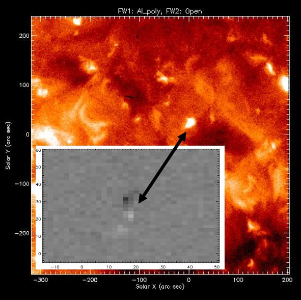
Figure 1: X-ray Image taken from XRT/Hinode on 19 December 2006 at 22:08 UT. Insert: the LOS component of the photospheric magnetic field in a 64 $\times$ 64 $arcsec^{2}$ horizontal plane taken from MDI/Soho, where white (black) spots correspond to upward (downward) directed Line-of-sight components of the photospheric magnetic field. The BP and the related magnetic field feature are indicated in the images.

Fourier filtering was applied to the LOS component of the magnetic field. By taking into account only the first eight Fourier modes, details of magnetic field structure smaller that 6 Mm are neglected. The extension of structures arising from smaller scale magnetic features would not extend higher up into the corona, they are dissipated at an early stage of the evolution in the highly collisional chromospheric plasma.

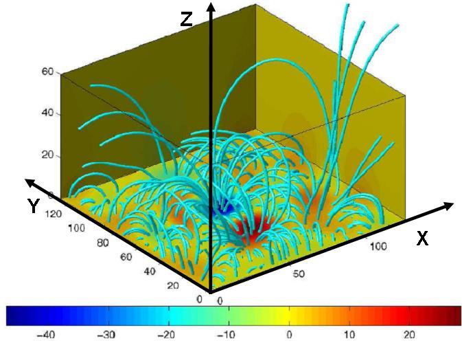
Figure 2: Potential magnetic field extrapolated from the filtered MDI magnetograms and used as initial configuration for the magnetic field in our simulation. The blue lines show the magnetic field lines. The color code depicts the LOS component of the magnetic field. Note that axes here are in terms of grid points, 64 in z direction and $128\times 128$ in x,y plane.

Fig. 2 shows a three-dimensional view of the magnetic field extrapolated from the photospheric boundary for the magnetic field observed at 22:17 UT on December 19, 2006. The blue lines show the magnetic field lines. The color code depicts the LOS component of the photospheric magnetic field. Magnetic fields directed upward from the photosphere are colored in red, downward directed in blue.

With the chosen normalization length of $L_{0}=500$ km, the box size in x and y direction correspond to 92.8 $L_{0}$ and the z direction extend to 30.9 $L_{0}$. The photospheric plasma velocities are obtained by applying the local-correlation-tracking(LCT) method November & Simon (1988) to the Fourier filtered LOS magnetic component of the photospheric magnetic field observed between 22:17 UT and 22:22 UT. The left panel of Fig. 3 shows the velocity pattern obtained by the LCT method. For the simulation we used incompressible velocity vortices to mimic the observed velocity pattern, as shown in the right panel of Fig. 3. Note that the interval chosen for the simulation starts a few hours after the time the BP first appeared in the X-ray images and that the bright point continues to glow a few more hours afterwards. During the whole simulation time interval the relative shear motion of the two main magnetic flux concentrations of opposite polarity is negligible.

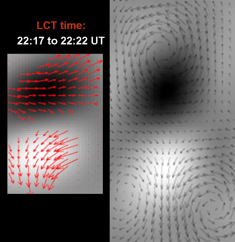
Figure 3: Horizontal plasma velocities in the photosphere. Left panel: velocities obtained by applying LCT technique to MDI magnetograms between 22:17 and 22:22 UT. The right panel shows the vortices that are used to approximate this motion in the simulation.

4 Simulation results

The simulation results are first shown in a plane at x = 45.7 (Fig. 2), which crossed through the center of the two main magnetic polarities. The vertical profile of the temperature is shown in Fig. 4 for t = 0 (top panel), 80 (middle panel) and 160 s (bottom panel). In $t=0$ we have a height dependent temperature as defined by the initial condition. At $t=80$ s the effects of plasma compression and expansion, together with Joule heating, shape the temperature profile. An arc of hot plasma is formed above the two opposite magnetic polarities. The increase in temperature in this layer is approximately 0.5 in normalized units, what corresponds to 36000 K. The region that is located just below it, however, experiences some drop in temperature. At $t=160$ s the arc of hot plasma leaves the simulation box and we are left with a corona in which the differences in temperature can reach one orders of magnitudes.

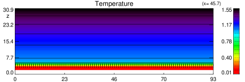
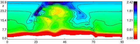
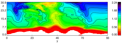
Figure 4: Temperature distribution in the vertical plane at x = 45.7 at the beginning (upper panel) and at t = 80 s and t = 160 s. Note the temperature in color bar in presented in terms of the normalization value.

Fig. 5 shows the parallel and perpendicular components of the current with respect to the magnetic field direction at t = 80 and t = 160s. It can be seen that enhanced current flows coincide well with the temperature increase. This would lead to an interpretation of the heating as being due to current dissipation only. However, as shown later, adiabatic heating can have an important contribution to temperature increase.

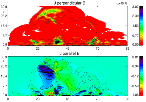
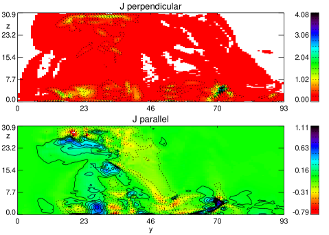
Figure 5: Parallel and perpendicular components of electrical current at t = 80 s (upper two panels) and t = 160 s (lower two panels) in the same diagnostic plane as in Fig.4. Note the enhancement in perpendicular current is located at the same place of the temperature maximum.

5 Energy balance

Let us now diagnose the different contributions to plasma heating in the BP region. First, in subsection 5.1, we discuss the overall global heating. In subsection 5.2 the dependence on the resistivity model is presented. Finally, the flux-tube heating is analyzed in subsection 5.3.

5.1 Global effect of current dissipation and compression

In order to understand the relative contribution of current dissipation and plasma compression to the coronal plasma heating in the BP region it is appropriate to analyze the pressure changes rewriting the Eq. 4 in terms of a continuity equation for the Temperature evolution. This leaves two source terms on the right hand side of the equation:

$$\frac{\partial T}{\partial t}+\@vec{\nabla}\cdot T\@vec{u}=-(\gamma-1)\ T\ \@vec{\nabla}\cdot\@vec{u}+(\gamma-1)\ \eta j^{2}/\rho$$ (12)

Let us first analyze the first case, where an anomalous resistivity is used when the current carrier velocity exceeds a critical value. Fig. 6 shows the resulting distribution of $-(\gamma-1)\ T\ \@vec{\nabla}\cdot\@vec{u}$ in the vertical diagnostic plane. This way we have a proxy for temperature changes associated to pressure compression and expansion.

Adiabatic heating has an important role on the formation of the high temperature arc that propagates upward towards the top boundary. It is also due to expansion that temperature decreases below this hot arc.

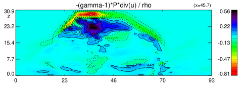
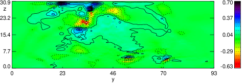
Figure 6: Adiabatic cooling/heating rate after 80 s and 160 s in the plane x = 45.7, according to the first term in the r.h.s of Eq. 11 over density, ($-(\gamma-1)T\nabla\cdot u<0$).

The values of second term in the right hand side of the Eq. 11, $(\gamma-1)\ \eta j^{2}/\ \rho$, is shown in Fig. 7 in the plane x = 45.7 at t = 80s and t = 160s. By comparison with the compressional part the contribution of the Joule heating appears to be negligible. For a better comparison the contribution of the two terms in the right hand side of the Eq. 11 in the temperature evaluation, the horizontal view is shown at the height of transition region in two different instance of time, t = 80 s in left and t = 160 s in the right panel of Fig. 8.

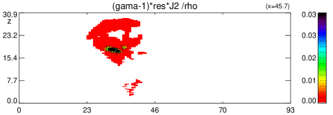
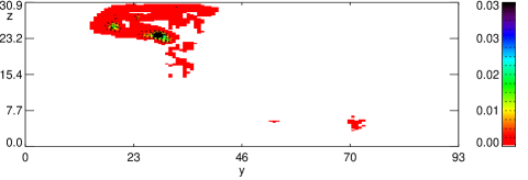
Figure 7: Joule heating rate, (second term in the r.h.s of Eq. 12, divided by density), after 80 s and 160 s in the plane x = 45.7.

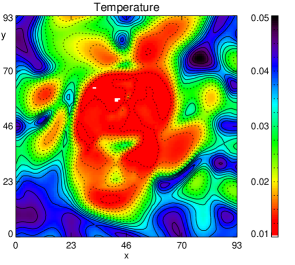
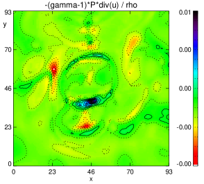
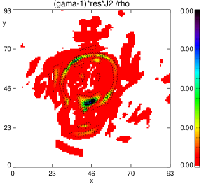
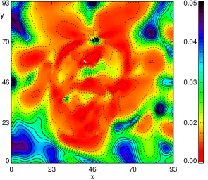
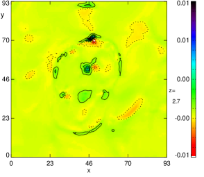
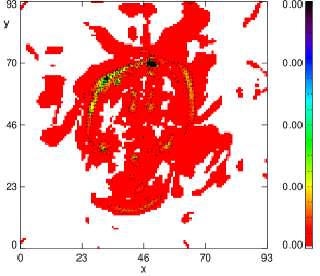
Figure 8: Temperature, first and second terms of Eq. 12 over density, in the left, middle and right panels, respectively. The result is shown at a horizontal plane in transition region at two instance of time, t = 80s in top and t = 160s in the bottom panels.

In the following, we will analyze in some more detail to what degree compression and Joule heating contribute to the evolution of the temperature. For this sake and in order to study the role of the forces involved in the energy conversion process, we performed a volume integration of the time rates of change of kinetic, magnetic and thermal energies in the simulation box above the chosen Bright Point region. Our approach is similar to Birn et al. (2009) when they used energy transport equations to analyze the properties of energy conversions associated with a reconnection process. The contribution of different terms in the energy transport process can be studied from the following equations:

$$\frac{d\varepsilon_{kin}}{dt}=-\frac{1}{2}\int_{S_{V}}\rho u^{2}\@vec{u}\cdot d\@vec{s}+\int_{V}(-\@vec{u}\cdot\nabla p+\@vec{u}\cdot\@vec{j}\times\@vec{B})d^{3}v$$ (13)

$$\frac{d\varepsilon_{mag}}{dt}=-\frac{1}{\mu_{0}}\int_{S_{V}}(-\@vec{u}\@vec{B}^{2}+(\@vec{u}\cdot\@vec{B})\@vec{B}-\eta\@vec{j}\times\@vec{B})\cdot d\@vec{s}$$ (14)

$$+\int_{V}(-\@vec{u}\cdot\@vec{j}\times\@vec{B}-\eta\@vec{j}^{2})d^{3}v$$

$$\frac{d\varepsilon_{th}}{dt}=-\frac{\gamma}{\gamma-1}\int_{S_{V}}p\@vec{u}\cdot d\@vec{s}+\int_{V}(\@vec{u}\cdot\nabla p+\eta\@vec{j}^{2})d^{3}v$$ (15)

Where $\varepsilon_{kin}$, $\varepsilon_{mag}$ and $\varepsilon_{th}$ denote kinetic, $\rho u^{2}/2$ , magnetic, $\@vec{B}^{2}/2\mu_{0}$, and thermal, $P/(\gamma-1)$, energies, respectively. The volume integrals (second term on the right-hand side) in these equations represent the energy conversion from one form into the another. This energy conversion are explicitly written in terms of the work done by Lorentz force, pressure gradient force and Joule dissipation, (left panel of Fig. 9). Note that the initial spike in the Lorentz force is in part caused by numerical discretization errors and in part by the onset of photospheric footpoint motion. The initial oscillations are damped substantially during, approximately, two Alfvén times, followed by a state of an approximate force balance. This effect was found to be smaller in a run where footpoint motion was not included. The initial perturbation has a minor effect on the initial extrapolated magnetic field, it does not affect the currents and Lorentz forces at a later times.

The surface integrals are also needed to obtain the energy rates, when they indicate the transport of each of the three form of energies. With the chosen boundary condition however, the values of these surface integrals are zero at the lower boundary. They compensate each other through the side boundaries of the simulation box as well. At the upper boundary however, one needs to consider the contribution of this surface integrals in the rate of energy transfer. This means $\textbf{E}\times\textbf{B}$, $P\textbf{u}$ and $\rho u^{2}\textbf{u}$ for the transport of magnetic, kinetic and thermal energies, respectively. The values of these terms at the upper boundary are shown in Fig. 10. One can see that the contribution due to these terms is insignificant, so it would be a good approximation to consider only the volume integrals for the change in the energy rates.

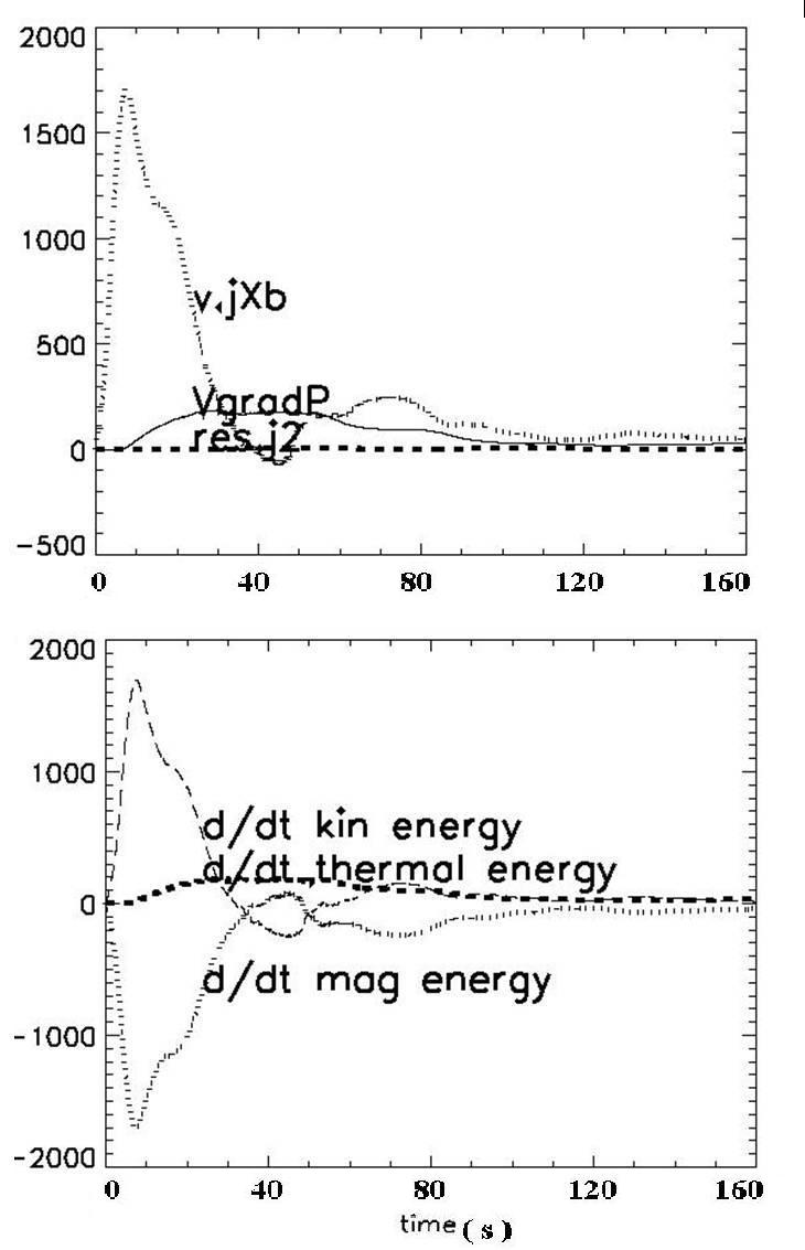
Figure 9: Rates of the contribution to the total energy changes, (bottom panel). Different contributions to the changes of the energy, (top panel).

The changes in energy rates are shown in the right panel of Fig. 9, the forces responsible for these changes are depicted in the left panel of the Figure. As one can see by comparing the two panels the magnetic energy is transferred to kinetic energy almost completely via the work done by the Lorentz force that accelerates the plasma. It is an intermediate step however, followed by the work done by pressure gradient force that converts kinetic energy into thermal energy. This decelerates the plasma motion until, finally, the Lorentz force is balanced. The direct transformation of magnetic energy to thermal energy (Joule heating) is via Ohmic current dissipation, $\eta J^{2}$. A comparison of the energy conversions rates (see Fig. 9, right panel) however shows that Joule dissipation plays a minor role in the energy exchange process while the other contributions are orders of magnitudes larger. The minor role of Joule heating in comparison to adiabatic process in the increase of thermal energy was also found for the case of a solar flare by Birn et al. (2009), where they explained the compressional heating in two almost simultaneously steps: acceleration by Lorentz force and deceleration by pressure gradients.

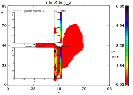
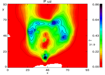
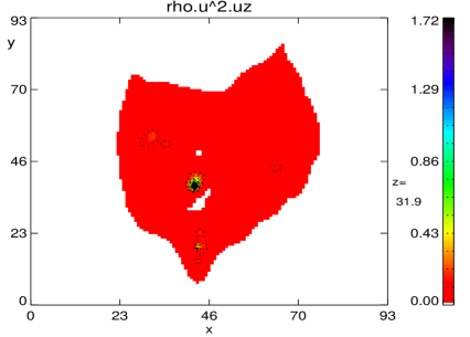
Figure 10: First term in the right hand side of the Eqs.12-14, (surface integrals) is shown in the upper boundary of the simulation box after 160 s.

5.2 Influence of different resistivity models

The previous calculation was based on an anomalous resistivity model with the current carrier velocity as a critical value for a local switch-on of additional resistivity. In order to better understand the influence of the resistivity we performed the simulation also with two other resistivity models, one that uses a current density dependent resistivity and another with constant resistivity respectively.

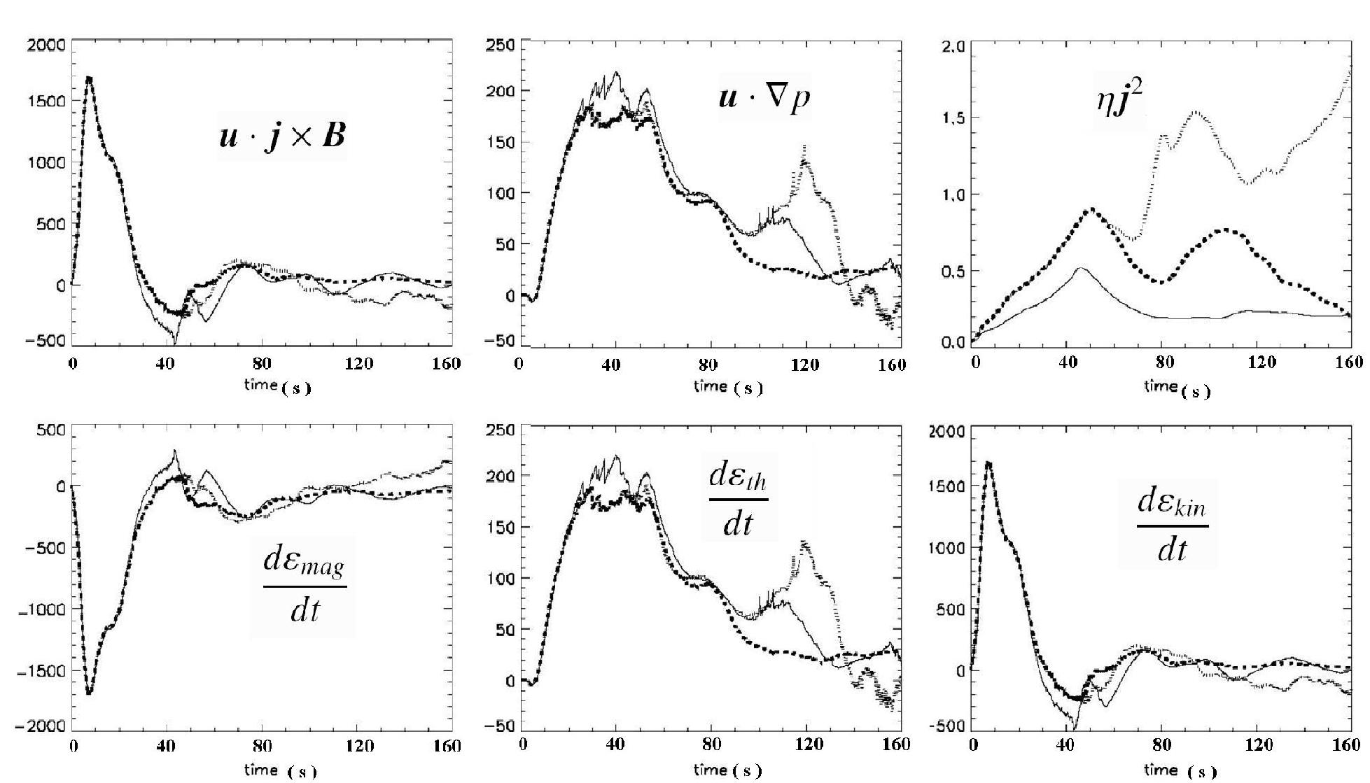
Figure 11: Energy change rates for three different resistivity models, (top panel). The bottom panel shows the work done by the Lorentz force, pressure gradient force and the Joule heating power. different lines correspond to anomalous current carrier dependent (dashed), anomalous current dependent (dotted) and constant (solid line) resistivity models.

Fig. 11 depicts the resulting energy conversion rates and the work done by the involved forces  v $\cdot\ J\times B$, v $\cdot\ \nabla P$ and by $\eta\ J^{2}$, for all the three resistivity models by using different line styles for the results obtained by using the different resistivity model. The results obtained for the three cases show that the resistivity model influences the dynamics of the system and the thermal energy rate mainly through the pressure gradient force. While magnetic and kinetic energy rates of change depend only weakly on the resistivity model, the rate of temperature change is significantly influenced. Nevertheless, independent on the used resistivity model the heating is due mainly to the work done by the pressure gradient force. At the same time the contribution of the Joule heating is about two orders of magnitude smaller (Note the scale of the plots in the top row.) We conclude that the adiabatic compression is the dominant effect in increasing temperature in the BP region in all three cases.

5.3 Flux tube heating

In order to locate the heating effect better it is appropriate to determine it for individual flux tubes, integrating along the magnetic field lines instead of taking values averaged over the whole simulation box as reported in the previous sections. In this integration one has to take into account the changing cross-section of flux tubes. This can be done by applying the concept of the differential flux tube volume $V=\int{B}^{-1}ds$, where ds indicates the step size along the field line. This way the flux conservation in a flux tube ($\Phi=A\times B=const.$) is taken into account by the proportionally of the cross-section to $B^{-1}$. Note that large flux tube volumes correspond to field line rising high into the corona or hitting regions of vanishing magnetic field. The energy is transported in accordance with the upward directed Poynting flux $E\times B$, enhanced magnetic tension is carried away by wave propagation.

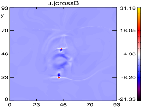
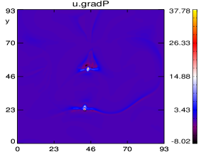
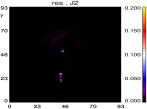
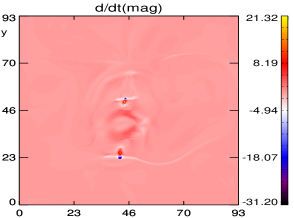
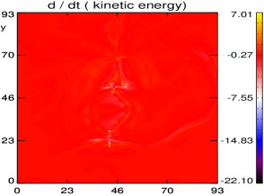
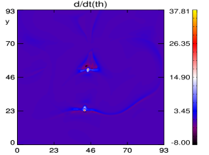
Figure 12: Integration along the field lines using the differential flux tube volume concept for the work done by Lorentz force, pressure gradient force and Joule heating, (top panel, from left to right), and the changes in rates of magnetic field change, the temperature and the kinetic energy, (bottom panel, from left to right) at t = 160s.

For the quantities described in section 5.1 the resulting flux tube integrated values are shown in Fig.  12 in the horizontal reference plane just above the transition region. The values reached indicate once more the negligible role of Joule heating by current dissipation for the thermal energy change in the bright point region compared to the dominant role of the pressure gradient force. Please note the different range of the plots in Figure 12 as indicated by the color bar. It also can be seen that the locations at which this force and also maximum rates of energy changes appear coincide. Furthermore, the same pattern has formed in the integration result of v $\cdot\ \nabla P$, v $\cdot\ J\times B$ and the rate of change of the different kinds of energy. This pattern can clearly be seen in the integration of total energy along the field lines (Fig.  13), which is the sum of the kinetic, magnetic and thermal energies:

$$\varepsilon=\varepsilon_{kin}+\varepsilon_{mag}+\varepsilon_{th}=\int_{V}\{\frac{1}{2}\rho u^{2}+\frac{1}{2\mu_{0}}B^{2}+\frac{p}{\gamma-1}\}d^{3}v$$

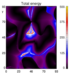
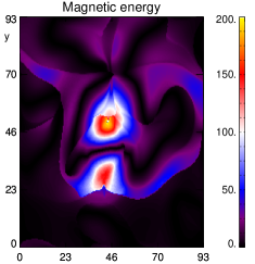
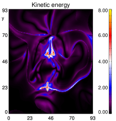
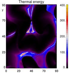
Figure 13: Results of integration along the magnetic field lines using the differential flux tube volume concept for total energy(top, left panel) and magnetic(top, right panel), kinetic(bottom, left panel) and thermal energies(bottom, right panel), at t = 160s.

The left panel of Fig. 14 shows the result of this integration for temperature and flux tube volume. The coincidence of the temperature enhancement with the maxima obtained in the flux tube integrated energy change rates and forces shows that the heat is provided by the plasma compression due to the Lorentz force.

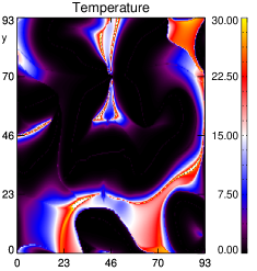
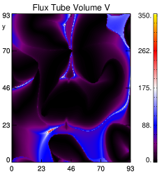
Figure 14: Temperature and flux tube volume, integrated along the magnetic field lines, at t = 160s.

Enhanced flux tube integrated values follow the same pattern as the BP. This indicates that the regions of enhanced temperatures correspond to the foot points of field lines leading to higher altitudes or to regions where the magnetic field vanishes. The plasma motion across these regions supplies the magnetic energy that is converted to thermal energy.

6 Summary and discussion

We have presented the results of heating processes in the region of an observed X-ray coronal bright point. In particular we have investigated the importance of the work done by adiabatic compression in comparison with Joule heating in the course of the dynamic evolution and heat production near the bright point.

The simulation shows that an arc-shaped structure of enhanced temperature forms that is 2-4 times hotter than the background plasma. This structure is located above the two main opposite photospheric magnetic flux concentration. It coincides with the location where the electrical current densities are maximum. The structures of temperature and current density enhancements, indeed, coincide.

We further examined the contribution of the Lorentz force, pressure gradient force and Joule heating performing volume integrals in the simulation box that determine the magnetic, kinetic and thermal energy change rates for three different resistivity models. We found that independent on the resistivity model magnetic energy was transformed to kinetic energy through the work done by Lorentz force. Kinetic energy in turn is converted to thermal energy due to pressure gradients that balance the Lorentz force.

A comparison of the effect of the three energy conversion through v $\cdot\ J\times B$, v $\cdot\ \nabla P$ and $\eta\ J^{2}$ show that adiabatic compression has an important role in temperature increase in the upper corona. This is not dependent on the resistivity model used in the simulation.

For a better understanding of the heating processes we utilized the concept of differential flux tube integration of the different contributions along the magnetic field lines. A quantitative comparison in the horizontal plane, from where the integration starts, shows that energy conversion rate, total energies and work done by Lorentz and pressure gradient forces are located in the same flux tubes, also temperature and flux tube volume are maximum at the same place.

We conclude that the conversion of magnetic energy to kinetic energy via the work done by the Lorentz force and from kinetic to thermal energy due to the work done against the pressure gradient force determine the heating of this bright point. We could show that plasma compression dominates the heating of the bright point. In contrast, the role of Joule dissipation appeared to be negligibly small. The temperature enhancement follows the same pattern. The fact that the pattern obtained by calculating flux volume integrals coincides with the one of temperature and energy change rates bring us to the conclusion that plasma motion at the footpoints of the flux tubes carries the energy upward and makes the flux tubes rise to the higher corona. The magnetic energy is converted to thermal energy until the plasma compression is balanced by the Lorentz force. In the local, flux-tube oriented consideration we also could see that the role of the Joule heating in these energy conversion processes was negligible and the heating of plasma in the bright point region is basically due to pressure gradient force.

First, the fact that Joule heating is weak in the corona was not entirely unexpected but it is quantitatively confirmed here. It is worth to remember that the necessary up-scaling of the resistivity and of the onset condition of micro-turbulent anomalous resistivity to the resolved by the MHD simulation grid scales does even overestimate the actual Joule heating. As a result Joule heating cannot be considered a viable process unless there is a convincing argument that the dissipation regions are volume filling to a much larger extend than the already large one used in the present model.
Second, the results demonstrate very clearly that compression is an important processes in the energy budget. It is not clear in how far compression can contribute to the overall coronal heating but it is certainly important for the local heating of BPs.
Third, in this context the nature and the consequences of plasma compression are worth some consideration. In ideal MHD adiabatic compression is reversible. But the consequent flux tube heating is, however, irreversible due to magnetic reconnection and other mixing processes. Magnetic reconnection, in particular, changes flux tube identities (magnetic connectivity) while flux tube entropy conservation requires ideal MHD in addition to appropriate boundary conditions. Local adiabatic compression becomes irreversible also due to other plasma transport processes like heat conduction and radiative cooling. These aspects will be separately investigated in a subsequent paper. Meanwhile the results presented here clearly demonstrate that in the overall energy budget plasma compression (and expansion) can play an important role in the heating of the corona.