Spectrum of the Wilson Dirac Operator at Finite Lattice Spacings

Abstract

We consider the effect of discretization errors on the microscopic spectrum of the Wilson Dirac operator using both chiral Perturbation Theory and chiral Random Matrix Theory. A graded chiral Lagrangian is used to evaluate the microscopic spectral density of the Hermitian Wilson Dirac operator as well as the distribution of the chirality over the real eigenvalues of the Wilson Dirac operator. It is shown that a chiral Random Matrix Theory for the Wilson Dirac operator reproduces the leading zero-momentum terms of Wilson chiral Perturbation Theory. All results are obtained for fixed index of the Wilson Dirac operator. The low-energy constants of Wilson chiral Perturbation theory are shown to be constrained by the Hermiticity properties of the Wilson Dirac operator.

I Introduction

In the continuum, low-lying spectra of the Dirac operator for theories with spontaneous chiral symmetry breaking have two equivalent descriptions. One is in terms of chiral Random Matrix Theory SV ; RMT ; RMT1 ; RMT2 , and the other one is in terms of a chiral Lagrangian LS ; DOTV ; SplitV . It is by now well-established how the two formulations are in one-to-one correspondence DOTV ; TV ; Basile , and that this is valid for all spectral correlation functions of the Dirac operator. Even single eigenvalue distributions can be derived in both formalisms, and have been shown to be equivalent AD . The equivalence is valid to leading order in a chiral counting scheme known as the $\epsilon$-regime or, in Random Matrix Theory terminology, the microscopic domain.

Apart from its conceptual value, the theory of low-lying Dirac operator spectra has been of quite practical use in lattice gauge theory. In fact, it serves multiple purposes, all relying on a QCD partition function that is formulated from the outset at finite four-volume $V$: (1) it can be used to establish spontaneous chiral symmetry breaking in a clean way, (2) it provides precise non-perturbative analytical predictions that can be used to test the chiral limit, and (3) it allows for a determination of low-energy constants by means of finite-volume scaling. So far these uses have been limited by the fact that violations due to finite lattice spacings, $a$, have been ignored. Such lattice artifacts evidently depend on the particular lattice discretization chosen. Following Symanzik’s program, corrections due to finite lattice spacings can, when they are sufficiently small, be analyzed in a continuum field theory language through the introduction of higher-dimensional operators in the Lagrangian. The corrections to the chiral Lagrangian that arise up to and including order $a^{2}$-effects for Wilson fermions have been analyzed in a series of papers SharpeSingleton ; RS ; BRS ; Aoki-spec ; Aoki-pion-mass ; Golterman:2005ie . For comprehensive reviews of effective field theory methods at finite lattice spacings, see, $e.g.$, ref. sharpe-nara ; Golterman .

It is then an obvious problem to investigate the effect of lattice-induced scaling violations on the spectral properties of the Wilson Dirac operator $D_{W}$ Sharpe2006 . In a recent Letter DSV , three of the present authors have taken up this issue and shown how the microscopic scaling regime can be phrased both in terms of the (graded) chiral Lagrangian and a modified chiral Random Matrix Theory that incorporates finite lattice spacing effects of Wilson fermions.

Although the Wilson Dirac operator is not Hermitian, the operator $D_{5}\equiv\gamma_{5}(D_{W}+m)$ is Hermitian, and much more convenient to work with in lattice QCD simulations. In this paper we analyze the microscopic spectrum of this operator. Contrary to the lattice QCD Dirac operator at $a=0$, its eigenvalues $\lambda_{k}^{5}(m)$ are not paired and are nontrivial functions of the quark mass.

There is a deep relation between the topology of gauge field configurations and the spectrum of the Dirac operator. Not only is the number zero eigenvalues equal to the difference of the number of right handed and left handed zero modes, because of level repulsion the Dirac spectrum near zero is affected in a universal way by the topological charge. As can be shown from spectral flow arguments (see, $e.g.$ SmitVink ; Itoh ; neuberger ; Edwards ; Hernandez ; Gattringer ; Hasenfratz ), the eigenvalues corresponding to the chiral modes at zero lattice spacing (when the Dirac operator is antihermitian) correspond to exactly real eigenvalues at nonzero lattice spacing. Additional pairs of real modes appear for increasing lattice spacing. However, the number of spectral flow lines, $\lambda_{k}^{5}(m)$, with an odd number of real zeros remains the same. We will identify the number of such flow lines as the index of the Dirac operator and study Dirac spectra for a fixed index. In the continuum limit this index, by the Atiyah-Singer index theorem becomes equal to the topological charge of the gauge field configurations. In Random Matrix Theory, this index is determined by the block structure of the Dirac matrix. All results in this paper are derived for fixed index of the Dirac operator. It is of course also possible to sum over all sectors with a given index.

In this paper we elaborate on and provide detailed derivations of results announced in the Letter DSV and the proceedings latNf0 . One of the simplifying features of that paper was that double-trace terms in the chiral Lagrangian were ignored (which can be justified based on large-$N_{c}$ arguments KL ). Here we compute their contribution to the microscopic spectrum directly from the chiral Lagrangian. We also show how double-trace terms can be included in the Wilson chiral Random Matrix Theory. We study in detail the $a\to 0$ and four-volume $V\to\infty$ limits of the analytical results. Furthermore, it is shown that the low-energy constants of Wilson chiral Perturbation Theory are constrained by a QCD inequality which follows from the Hermiticity properties of the Wilson Dirac operator. This constraint coincides precisely with the requirement of preservation of the Hermiticity properties of the Wilson Dirac operator. The constraints found are consistent with the existence of an Aoki phase. One important message from the calculations presented here is that the values of the low-energy constants of Wilson Chiral Perturbation Theory can be accurately determined by matching the predictions for the eigenvalue distributions to lattice data. Furthermore, our results describe analytically the eigenvalues that may cause numerical instabilities Luscher when approaching the chiral limit at finite lattice spacing with Wilson fermions.

The analysis of the Letter DSV has been extended in various other directions. We have obtained the distribution of the chirality over the real eigenvalues of the Wilson Dirac operator which is a lower bound for the distribution of the real eigenvalues. We also have obtained an upper bound which converges to the lower bound for small $a$. In the same limit the expressions for the microscopic spectral density of $D_{5}$ simplify and can be generalized to a nonzero number of flavors. We discuss the distribution of the tail states in the gap as well as a comparison with the scaling properties of such states as found in lattice simulations. We also perform a saddle point analysis of our analytical result and obtain a simple explicit expression for the gap of the Dirac spectrum.

The paper is organized as follows. After a brief review of relevant properties of the Wilson Dirac operator given in section II we define Wilson chiral Perturbation Theory at a fixed index of the Wilson Dirac Operator in section III. The derivation of the microscopic spectrum is given in section IV. It is followed by a discussion of various limits in section V. A chiral Random Matrix Theory for Wilson fermions is shown to reproduce Wilson chiral Perturbation Theory in the microscopic limit in section VI. Finally, before concluding, we discuss the relation between the low energy constants of the Wilson chiral Perturbation Theory and the Hermiticity properties of the Wilson Dirac operator. Some technical details are referred to Appendix A, Appendix B and Appendix C.

II Eigenvalues of the Wilson Dirac Operator

We start with a discussion of general properties of the Wilson Dirac operator. Some of these results have been discussed extensively in the literature (see, $e.g.$, refs. Itoh ; neuberger ; Edwards ; Hernandez ; Gattringer ; Sharpe2006 ), but are included here to make this paper self-contained.

The Wilson-Dirac operator will be denoted by $D=D_{W}+m$. The lowest order $a$ correction was introduced by Wilson,

$$D_{W}=\frac{1}{2}\gamma_{\mu}(\nabla_{\mu}+\nabla^{*}_{\mu})-\frac{1}{2}a\nabla^{*}_{\mu}\nabla_{\mu}.$$ (1)

It is written in terms of forward ($\nabla_{\mu}$) and backward ($\nabla^{*}_{\mu}$) covariant derivatives, and $m$ is the quark mass.

The Wilson Dirac operator, $D_{W}$, is not anti-Hermitian at non-zero lattice spacing. It retains only $\gamma_{5}$-Hermiticity:

$$D_{W}^{\dagger}=\gamma_{5}D_{W}\gamma_{5}.$$ (2)

The eigenvalues, $\lambda^{W}_{k}$, of $D_{W}$ are then either real or they occur in complex conjugate pairs. The $\gamma_{5}$-Hermiticity of $D_{W}$ implies that the operator

$$D_{5}\equiv\gamma_{5}(D_{W}+m)$$ (3)

is Hermitian. Since at non-zero lattice spacings $a$ the axial symmetry is lost ($\{D_{W},\gamma_{5}\}\neq 0$), the eigenvalues of $D_{5}$ do not occur in pairs of opposite sign.

The eigenvalues, $\lambda_{k}^{5}(m)$, of $D_{5}$ are nontrivial functions of $m$. If $\lambda_{k}^{5}(m_{c})=0$, then

$$\gamma_{5}(D_{W}+m_{c})\phi=0\quad\Rightarrow\quad D_{W}\phi=-m_{c}\phi,$$ (4)

so that the real eigenvalues of $D_{W}$ can be obtained from the zeros of $\lambda_{k}^{5}(m)$ with the corresponding eigenfunctions of $D_{5}$ and $D_{W}$ beeing identical at $m=m_{c}$. If we act with $D_{5}$ on the normalized eigenfunctions $\phi_{j}\equiv|j\rangle$ of $D_{W}$ we obtain

$$D_{5}\phi_{j}=\gamma_{5}(D_{W}+m)\phi_{j}=(-m_{c}+m)\gamma_{5}\phi_{j}.$$ (5)

For $m$ close to $m_{c}$

$$\gamma_{5}\phi_{j}=\langle j|\gamma_{5}|j\rangle\phi_{j}+\delta\phi,$$ (6)

with $\langle\delta\phi|j\rangle=0$ and $\delta\phi\sim O(m-m_{c})$. Therefore to $O(m-m_{c})$

$$\lambda_{j}^{5}(m)=(m-m_{c})\langle j|\gamma_{5}|j\rangle.$$ (7)

We thus find Itoh

$$\frac{d\lambda_{j}^{5}}{dm}=\langle j|\gamma_{5}|j\rangle+O(m-m_{c}).$$ (8)

When evaluated at $m=m_{c}$, ie. at $\lambda_{j}^{5}=0$, the slope is thus exactly given by the chirality

$$\frac{d\lambda_{j}^{5}}{dm}\Big{|}_{m=m_{c}}=\langle j|\gamma_{5}|j\rangle.$$ (9)

Furthermore, it can be shown Itoh that the chirality of the eigenfunctions

$$\chi_{j}\equiv\langle j|\gamma_{5}|j\rangle$$ (10)

vanishes for complex eigenvalues of $D_{W}$ but is generally nonzero for real eigenvalues.

To compute the spectral density $\rho_{5}$ of $D_{5}$ we introduce a source $z$ that couples to $\bar{\psi}\gamma^{5}\psi$. The operator entering in the fermion determinant is then given by

$$\gamma_{5}(D_{W}+m)+z=D_{5}+z,$$ (11)

and the resolvent of $D_{5}$ is defined by

$$G(z)\equiv\left\langle{\rm Tr}\left(\frac{1}{D_{5}+z-i\epsilon}\right)\right\rangle=\left\langle\sum_{k}\frac{1}{\lambda^{5}_{k}+z-i\epsilon}\right\rangle,$$ (12)

where $\lambda^{5}_{k}$ are the eigenvalues of $D_{5}$. The density of eigenvalues of $D_{5}$ then follows from

$$\rho_{5}(\lambda^{5},m;a)=\left\langle\sum_{k}\delta(\lambda^{5}_{k}-\lambda^{5})\right\rangle=\frac{1}{\pi}{\rm Im}[G(-\lambda^{5})]_{\epsilon\to 0}.$$ (13)

The resolvent (12) is a partially quenched chiral condensate. We will compute it by means of the graded technique, where the unphysical ’valence’ determinant is canceled by an inverse determinant after differentiation with respect to the source . In order to be able to write the inverse determinant as a bosonic integral, it is essential that an infinitesimal increment is added to a Hermitian operator Golterman:2005ie .

We also consider the chiral condensate corresponding to the regularization introduced in Eq. (12)

$$\Sigma(m)\equiv\left\langle{\rm Tr}\frac{1}{D_{W}+m-i\epsilon\gamma_{5}}\right\rangle.$$ (14)

Care has to be taken in order to relate $\Sigma(m)$ to the spectrum of $D_{W}$. The discontinuity of $\Sigma(m)$ across the real axis is given by

$$\rho_{\chi}(m) \equiv \frac{1}{2\pi i}\left\langle{\rm Tr}\left[\frac{1}{(D_{W}+m)-i\epsilon\gamma_{5}}-\frac{1}{(D_{W}+m)+i\epsilon\gamma_{5}}\right]_{\epsilon\to 0}\right\rangle$$ (15)

$$= \frac{1}{2\pi i}\left\langle{\rm Tr}\left[\frac{\gamma_{5}}{\gamma_{5}(D_{W}+m)-i\epsilon}-\frac{\gamma_{5}}{\gamma_{5}(D_{W}+m)+i\epsilon}\right]_{\epsilon\to 0}\right\rangle.$$

This expression can be rewritten in terms of eigenvalues and the normalized eigenfunctions $|k\rangle$ of $D_{5}$ (recall that for $\lambda^{5}_{k}=0$ the eigenfunctions of $D_{5}$ merge with that belonging to a real mode of $D_{W}$)

$$\rho_{\chi}(m) = \frac{1}{\pi}\left\langle\sum_{k}\frac{\epsilon\ \langle k|\gamma_{5}|k\rangle}{(\lambda^{5}_{k}(m))^{2}+\epsilon^{2}}\Big{|}_{\epsilon\to 0}\right\rangle$$ (16)

$$= \left\langle\sum_{k}\delta(\lambda_{k}^{5}(m))\ \langle k|\gamma_{5}|k\rangle\right\rangle,$$

$$= \left\langle\sum_{\lambda_{k}^{W}\in{\mathbb{R}}}\frac{1}{|d\lambda_{k}^{5}/dm|}\delta(\lambda_{k}^{W}+m)\langle k|\gamma_{5}|k\rangle\right\rangle,$$

where $\lambda_{k}^{W}$ are the eigenvalues of $D_{W}$. Using Eq. (9) this can be written as

$$\rho_{\chi}(\lambda^{W})=\left\langle\sum_{\lambda_{k}^{W}\in{\mathbb{R}}}\delta(\lambda_{k}^{W}+\lambda^{W})\,{\rm sign}(\langle k|\gamma_{5}|k\rangle)\right\rangle.$$ (17)

This shows that $\rho_{\chi}$ is the distribution of the chiralities over the real eigenvalues of $D_{W}$. Integrating this expression over $\lambda^{W}$ we obtain

$$\int\rho_{\chi}(\lambda^{W})d\lambda^{W} = \left\langle\sum_{\lambda_{k}^{W}\in{\mathbb{R}}}{\rm sign}(\langle k|\gamma_{5}|k\rangle)\right\rangle.$$ (18)

This is the average index of the Dirac operator. The index for a given gauge field configuration is defined by

$$\nu=\sum_{\lambda_{k}^{W}\in{\mathbb{R}}}{\rm sign}(\langle k|\gamma_{5}|k\rangle).$$ (19)

Since the real modes of $D_{W}$ correspond to the vanishing eigenvalues of $D_{5}$ we also consider $\rho_{5}(\lambda^{5}=0,m)$. A similar calculation as above results in

$$\rho_{5}(\lambda^{5}=0,m;a)=\left\langle\sum_{\lambda_{k}^{W}\in{\mathbb{R}}}\frac{\delta(\lambda_{k}^{W}+m)}{|\langle k|\gamma_{5}|k\rangle|}\right\rangle.$$ (20)

Because $|\langle k|\gamma_{5}|k\rangle|\leq 1$ we have the inequality (also valid for fixed index)

$$\rho_{\chi}(\lambda^{W})\leq\rho_{\rm real}(\lambda^{W})\leq\rho_{5}(\lambda^{5}=0,m=\lambda^{W};a),$$ (21)

where

$$\rho_{\rm real}(\lambda^{W})\equiv\left\langle\sum_{\lambda_{k}^{W}\in{\mathbb{R}}}\delta(\lambda_{k}^{W}+\lambda^{W})\right\rangle.$$ (22)

As a special case the average number, $\langle n_{\rm real}\rangle$, of real eigenvalues of $D_{W}$ for gauge field configurations with index $\nu$ is bounded by

$$\int d\lambda^{W}\,\rho^{\nu}_{\chi}(\lambda^{W})=\nu\ \leq\ \langle n_{\rm real}\rangle\ \leq\ \int dm\,\rho^{\nu}_{5}(\lambda^{5}=0,m).$$ (23)

III Wilson chiral Perturbation Theory

The operators contributing to Wilson chiral Perturbation Theory have been considered in a series of papers SharpeSingleton ; RS ; BRS . It is constructed in terms of a double expansion in both the usual parameters of continuum chiral Perturbation Theory and the lattice spacing $a$. Depending on which counting scheme one uses, various terms contribute to a given order Shindler:2009ri ; Bar:2008 ; Bar:2010 . We concentrate on the microscopic limit, the $\epsilon$-regime, in which the combinations

$$mV,\quad zV,\quad a^{2}V$$ (24)

are kept fixed in the infinite-volume limit $V\to\infty$. To leading order in these quantities, the low energy partition function for lattice QCD with Wilson fermions then reduces to a unitary matrix integral. Up to the infinite-volume chiral condensate $\Sigma$ and three low-energy constants determined by the discretization errors of Wilson lattice QCD, this integral is completely determined by symmetry arguments.

Since we are computing quantities up to and including ${\cal O}(a^{2})$ effects, it is important that all effects to this order are contained in the on-shell effective Symanzik action including ${\cal O}(a^{2})$ terms. This problem has been analyzed in detail by Sharpe for the $p$-counting-scheme Sharpe2006 . Here we reconsider the argument for the $\epsilon$-regime. One correction to relevant continuum operators corresponds to $a^{2}\bar{\psi}(x)\gamma^{5}\nabla_{\mu}^{2}\psi(x)$ Sharpe2006 . In the $\epsilon$-regime, such terms are suppressed by $1/\sqrt{V}$ with respect to the leading terms and need to be considered only at higher orders in the expansion. Additional lattice artifacts of potential ${\cal O}(a^{2})$ in the form of contact terms have been analyzed in ref. Sharpe2006 , and they are similarly suppressed.

As stressed by Leutwyler and Smilga LS , the topological charge of gauge field configurations plays an important role in the microscopic spectrum of the continuum theory. The $\nu$ zero modes of the Dirac operator distort the eigenvalue spectrum of the non-zero modes and lead to distinct predictions in sectors of fixed $\nu$. Likewise it is natural to study the microscopic spectral density of the Wilson Dirac operator for fixed index $\nu$. At the level of the chiral Lagrangian it is a priori far from obvious how to implement the projection onto sectors corresponding to a fixed index of $D_{W}$. Quite remarkably, such a projection can be achieved through a Fourier transform DSV : We decompose the partition function as

$$Z_{N_{f}}(m,z;a)=\sum_{\nu}Z_{N_{f}}^{\nu}(m,z;a)$$ (25)

with

$$Z_{N_{f}}^{\nu}(m,z;a) = \int_{U(N_{f})}dU\ {\det}^{\nu}U\ e^{V{\cal L}(U)}.$$ (26)

The Lagrangian ${\cal L}(U)$ is defined by

$${\cal L}(U) = \frac{1}{2}(m+z)\Sigma{\rm Tr}U+\frac{1}{2}(m-z)\Sigma{\rm Tr}U^{\dagger}$$

$$-a^{2}W_{6}[{\rm Tr}\left(U+U^{\dagger}\right)]^{2}-a^{2}W_{7}[{\rm Tr}\left(U-U^{\dagger}\right)]^{2}-a^{2}W_{8}{\rm Tr}(U^{2}+{U^{\dagger}}^{2}).$$

Below we will demonstrate that in the microscopic domain this corresponds to an ensemble of gauge field configurations for which the index of $D_{W}$ as defined by Eq. (19) is equal to $\nu$. The partitioning into sectors of fixed $\nu$ corresponds at the level of the unitary group integral to writing an $SU(N_{f})$ integral as an infinite sum of $U(N_{f})$ integrals.

In the Lagrangian (III), $\Sigma$ is the usual infinite-volume chiral condensate while $W_{6}$, $W_{7}$ and $W_{8}$ are low-energy constants that quantitatively determine the discretization errors of Wilson fermions. The terms proportional to $W_{6}$ and $W_{7}$ are believed to be suppressed in the large $N_{c}$ limit KL , and they were not included in ref. DSV . Here we include the effect of these terms explicitly. To lighten the notation, we introduce the scaling variables

$$\hat{m}\equiv m\Sigma V,\quad\hat{z}\equiv z\Sigma V,\quad\hat{a}_{i}^{2}\equiv a^{2}W_{i}V$$ (28)

with $i=6,7,8$.

IV Graded Generating Function

To obtain the distribution, $\rho_{\chi}^{\nu}$, of the chirality over the real eigenvalues of $D_{W}$ and $\rho_{5}^{\nu}$ at fixed index $\nu$ we will use the graded method. The generating function in this case takes the form

$${\cal Z}^{\nu}_{N_{f}+1|1}(m,m^{\prime},z,z^{\prime};a)=\int({\rm d}A_{\mu})_{\nu}\det(D_{W}+m)^{N_{f}}\frac{\det(D_{W}+m+\gamma_{5}z)}{\det(D_{W}+m^{\prime}+\gamma_{5}(z^{\prime}-i\epsilon))}\ \mbox{e}^{-S_{\rm YM}},$$ (29)

and we have two spectral resolvents

$$\Sigma^{\nu}(m;a)=-\lim_{m^{\prime}\to m}\frac{d}{dm^{\prime}}{\cal Z}^{\nu}_{N_{f}+1|1}(m,m^{\prime},z=0,z^{\prime}=0;a),$$ (30)

and

$$G^{\nu}(z,m;a)=-\lim_{z^{\prime}\to z}\frac{d}{dz^{\prime}}{\cal Z}^{\nu}_{N_{f}+1|1}(m,m,z,z^{\prime};a).$$ (31)

Note that the $N_{f}$ physical quark flavors are not coupled to the source $z$.

The presence of fermionic as well as bosonic quarks in this generating function gives rise to a graded structure (“supersymmetry”) of the corresponding chiral Lagrangian

$$Z^{\nu}_{N_{f}+1|1}({\cal M},{\cal Z};\hat{a}_{i}) = \int dU\ {\rm Sdet}(U)^{\nu}$$

$$\times e^{i\frac{1}{2}{{\rm STr}}({\cal M}[U-U^{-1}])+i\frac{1}{2}{{\rm STr}}({\cal Z}[U+U^{-1}])+\hat{a}_{6}^{2}[{{\rm STr}}(U-U^{-1})]^{2}+\hat{a}_{7}^{2}[{{\rm STr}}(U+U^{-1})]^{2}+\hat{a}_{8}^{2}{{\rm STr}}(U^{2}+U^{-2})},$$

where ${\cal M}\equiv{\rm diag}(\hat{m}\ldots\hat{m},\hat{m},\hat{m}^{\prime})$ and ${\cal Z}\equiv{\rm diag}(0\ldots 0,\hat{z},\hat{z}^{\prime})$, with ${\rm Im}(\hat{z}^{\prime})<0$. The integration is over the maximum Riemannian graded submanifold of $Gl(N_{f}+1|1)$ DOTV (see DOTV ; Efetov for notation and more on the graded method). For $N_{f}=0$ we will use the parametrization

$$U = \left(\begin{array}[]{cc}e^{i\theta}&0\\ 0&e^{s}\end{array}\right)\exp\left(\begin{array}[]{cc}0&\alpha\\ \beta&0\end{array}\right).$$ (37)

If we could $derive$ this partition function directly from the microscopic theory we would end up with $convergent$ integrals. Relying only on symmetry arguments is not sufficient to obtain the partition function, and it can only be equivalent to the microscopic partition function if the integrations are convergent. For fermionic integrals convergence is not an issue, but bosonic integrals necessarily have to be convergent.

In DOTV the graded partition function was evaluated for the anti-Hermitian Dirac operator with positive mass and $\hat{a}_{i}=0$ and $\hat{z}=0$. The term relevant for the convergence of the integral was $\exp(-\hat{m}\cosh s)$ so that the generating function is defined for $\hat{m}$ on the imaginary axis with a positive real infinitesimal increment, and can be used to calculate the spectral density localized on the imaginary axis. We could also have calculated the spectrum of $\gamma_{5}D$ by including the source term $\hat{z}\gamma_{5}$. This would have resulted in the bosonic integrand $\exp[-\hat{m}\cosh s-\hat{z}\sinh s]$. The corresponding integral can be continued analytically to the entire real $\hat{z}$-axis by shifting the $s$-integration by $s\to s\pm\pi i/2$ with the sign determined by the imaginary part of $\hat{z}$. This transformation can be accomplished by $U\to iU$ for ${\rm Im}(\hat{z})<0$ and by $U\to-iU$ for ${\rm Im}(\hat{z})>0$. The expression (IV) is thus valid for ${\rm Im}(\hat{z})<0$.

Next we consider the partition function with $\hat{a}_{i}^{2}\neq 0$. Let us first consider the case that $\hat{a}_{6}=\hat{a}_{7}=0$, and we consider the partition function as an analytical function of $\hat{a}_{8}^{2}$. The partition function (IV) is analytic in $\hat{a}_{8}^{2}$ for ${\rm Re}\,\hat{a}_{8}^{2}>0$, whereas the partition function of Ref. DOTV can only be continued to ${\rm Re}\,\hat{a}_{8}^{2}<0$. Depending on whether we consider the spectrum of $D_{W}$ or $\gamma_{5}D_{W}$ the partition function can be analytically continued to a different part of the complex $\hat{a}_{8}^{2}$-plane. Below we will argue that the physically interesting parameter domain is ${\rm Re}\,\hat{a}_{8}^{2}>0$, which is accessible for the integration contours of Eq. (IV) valid for the evaluation of the spectrum of $D_{5}$. Given this parametrization, the partition function is defined in only a subset of the complex $\hat{a}_{6}$ and $\hat{a}_{7}$ plane. For real constants the condition is that $\hat{a}_{8}^{2}-\hat{a}_{7}^{2}-\hat{a}_{6}^{2}>0$. Notice that in order to correspond to the QCD partition function, the limit $\hat{a}_{k}\to 0$ should be regular.

We will now explicitly work out the generating function (IV) in the quenched case where $N_{f}=0$. In order to do so we will use the parametrization Eq. (37) which has a flat measure DOTV . In this representation the generating function with $\hat{m}>0$ and ${\rm Im}(\hat{z}^{\prime})<0$ becomes (after $\alpha$ and $\beta$ are integrated out)

$$Z^{\nu}_{1|1}(\hat{m},\hat{m}^{\prime},\hat{z},\hat{z}^{\prime};\hat{a}_{i})$$

$$= \int_{-\infty}^{\infty}ds\int_{-\pi}^{\pi}\frac{d\theta}{2\pi}\ e^{(i\theta-s)\nu}\exp[-\hat{m}\sin(\theta)-i\hat{m}^{\prime}\sinh(s)+i\hat{z}\cos(\theta)-i\hat{z}^{\prime}\cosh(s)$$

$$+4\hat{a}_{6}^{2}(-i\sin(\theta)+\sinh(s))^{2}+4\hat{a}_{7}^{2}(\cos(\theta)-\cosh(s))^{2}+2\hat{a}_{8}^{2}(\cos(2\theta)-\cosh(2s))]$$

$$\times\big{(}-\frac{\hat{m}}{2}\sin(\theta)+i\frac{\hat{m}^{\prime}}{2}\sinh(s)+i\frac{\hat{z}}{2}\cos(\theta)+i\frac{\hat{z}^{\prime}}{2}\cosh(s)$$

$$\quad-4(\hat{a}_{6}^{2}+\hat{a}_{7}^{2})(\sin^{2}(\theta)+\sinh^{2}(s))+2\hat{a}_{8}^{2}(\cos(2\theta)+\cosh(2s)+e^{i\theta+s}+e^{-i\theta-s})\big{)}.$$

The $s$-integral is convergent for $\hat{a}_{8}^{2}-\hat{a}_{6}^{2}-\hat{a}_{7}^{2}>0$. In this case it is easily checked numerically that $Z_{1|1}(\hat{m},\hat{m},\hat{z},\hat{z};\hat{a})=1$, as required by the definition of the generating function. We discuss the convergence criterion in detail in section VII.2 below.

IV.1 The Microscopic distribution of the chirality over the real eigenvalues of $D_{W}$

In this section we show that the parameter $\nu$ in the chiral Lagrangian is the index of the Dirac operator $D_{W}$. Since we already have computed the generating function (IV) the condensate defined in Eq. (14) can be expressed as

$$\Sigma^{\nu}(\hat{m};\hat{a}_{i}) \equiv -\lim_{{\hat{m}}^{\prime}\to\hat{m}}\frac{d}{d\hat{m}^{\prime}}Z^{\nu}_{1|1}(\hat{m},{\hat{m}}^{\prime},\hat{z}=0,\hat{z}^{\prime}=-i\epsilon;\hat{a}_{i}).$$ (39)

This corresponds to a resolvent regulated with $i\epsilon\gamma_{5}$ instead of $i\epsilon$, and as was discussed in section II, it has quite different properties with a discontinuity that does not give the spectral density but rather the distribution $\rho^{\nu}_{\chi}$ of the chirality over the real eigenvalues of $D_{W}$ given in Eq. (17). It follows from (IV) that for Im$(\hat{z}^{\prime}=\hat{z})<0$

$$\Sigma^{\nu}(\hat{m};\hat{a}_{i}) = -\int_{-\infty}^{\infty}ds\int_{-\pi}^{\pi}\frac{d\theta}{2\pi}\ \sin(\theta)e^{(i\theta-s)\nu}\exp[-\hat{m}\sin(\theta)-i\hat{m}\sinh(s)-\epsilon\cosh s$$ (40)

$$+4\hat{a}_{6}^{2}(-i\sin(\theta)+\sinh(s))^{2}+4\hat{a}_{7}^{2}(\cos(\theta)-\cosh(s))^{2}+2\hat{a}_{8}^{2}(\cos(2\theta)-\cosh(2s))]$$

$$\times\Big{(}-\frac{\hat{m}}{2}\sin(\theta)+i\frac{{\hat{m}}}{2}\sinh(s)-4(\hat{a}_{6}^{2}+\hat{a}_{7}^{2})(\sin^{2}(\theta)+\sinh^{2}(s))$$

$$+2{\hat{a}}_{8}^{2}(\cos(2\theta)+\cosh(2s)+e^{i\theta+s}+e^{-i\theta-s})+\frac{1}{2}\Big{)}.$$

The discontinuity of this resolvent is equal to microscopic limit of the distribution of the chirality over the real eigenvalues of $D_{W}$ defined in Eq. (17),

$$\rho_{\chi}^{\nu}(\lambda^{W};\hat{a}_{i})=\left\langle\sum_{\lambda_{k}^{W}\in{\mathbb{R}}}\delta(\lambda_{k}^{W}+\lambda^{W})\,{\rm sign}[\langle k|\gamma_{5}|k\rangle]\right\rangle=\frac{1}{\pi}{\rm Im}[\Sigma^{\nu}(\hat{m}=\lambda^{W};\hat{a}_{i})].$$ (41)

It can be verified numerically that with the resolvent (40)

$$\int\rho_{\chi}^{\nu}(\lambda^{W};\hat{a}_{i})d\lambda^{W}=\nu.$$ (42)

This demonstrates that the sectors introduced in Eq. (26) correspond to a Dirac operator $D_{W}$ with index $\nu$, as defined in (19).

In Fig. 1 we plot the distribution of the chiralities over the real eigenvalues of $D_{W}$, $\rho_{\chi}^{\nu}(\lambda^{W},\hat{a}_{i})$, for $\nu=1,2,3$ for $\hat{a}^{2}_{8}=0.2$ and $\hat{a}_{6}=\hat{a}_{7}=0$. For this value of $\hat{a}_{8}$ additional pairs of real eigenvalues appear only rarely and $\rho_{\chi}^{\nu}(\lambda^{W},\hat{a}_{i})$ is a good approximation to the density of the real modes of $D_{W}$. Indeed, the presence of $\nu$ real eigenvalues is clearly visible. As we will show below, we can make an even more precise description of this in the limit of very small $\hat{a}_{8}$. In that limit we have $\nu$ real modes which turn out to be described by the $|\nu|\times|\nu|$ Gaussian Unitary Ensemble of Random Matrix Theory.

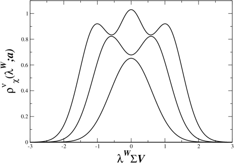
Figure 1: The quenched distribution of the chirality over the real modes of $D_{W}$ plotted for $\nu=1,2$ and $3$ with $\hat{a}_{8}=0.2$. For the plot we have chosen $\hat{a}_{6}=\hat{a}_{7}=0$. The real modes repel each other, making the preferred locations of the eigenvalues clearly visible.

IV.2 The Microscopic Spectrum of $D_{5}$

In the continuum ($a=0$) the eigenvalues $i\lambda_{k}$ of $D_{W}$ and eigenvalues $x_{k}$ of $D_{5}$ are related to each other through $(\lambda_{k}^{W})^{2}=(\lambda_{k}^{5})^{2}-m^{2}$. In this case, the microscopic eigenvalue density of $D_{5}$,

$$\rho_{5}^{\nu}(\lambda^{5}>\hat{m},\hat{m};\hat{a}_{i}=0)=\frac{\lambda^{5}}{\sqrt{(\lambda^{5})^{2}-\hat{m}^{2}}}\rho^{\nu}(\sqrt{(\lambda^{5})^{2}-\hat{m}^{2}})$$ (43)

follows from that of $D_{W}$. In the quenched case we have RMT ; DOTV

$$\rho^{\nu}(\lambda)=\frac{\lambda}{2}\left[J_{\nu}(\lambda)^{2}-J_{\nu+1}(\lambda)J_{\nu-1}(\lambda)\right].$$ (44)

To obtain the eigenvalue density, $\rho_{5}^{\nu}$, of the Hermitian Wilson Dirac operator $D_{5}$ for non-zero values of $\hat{a}$ we first evaluate the resolvent

$$G^{\nu}(\hat{z},\hat{m};\hat{a}_{i}) \equiv -\lim_{{\hat{z}}^{\prime}\to\hat{z}}\frac{d}{d\hat{z}^{\prime}}Z^{\nu}_{1|1}(\hat{m},\hat{m},\hat{z},{\hat{z}}^{\prime}-i\epsilon;\hat{a}_{i})$$ (45)

to find

$$G^{\nu}(\hat{z},\hat{m};\hat{a}_{i}) = \int_{-\infty}^{\infty}ds\int_{-\pi}^{\pi}\frac{d\theta}{2\pi}\ i\cos(\theta)e^{(i\theta-s)\nu}$$

$$\times\exp[-\hat{m}\sin(\theta)-i\hat{m}\sinh(s)+i\hat{z}\cos(\theta)-i(\hat{z}-i\epsilon)\cosh(s)$$

$$+4\hat{a}_{6}^{2}(-i\sin(\theta)+\sinh(s))^{2}+4\hat{a}_{7}^{2}(\cos(\theta)-\cosh(s))^{2}+2\hat{a}_{8}^{2}(\cos(2\theta)-\cosh(2s))]$$

$$\times\big{(}-\frac{\hat{m}}{2}\sin(\theta)+i\frac{\hat{m}}{2}\sinh(s)+i\frac{\hat{z}}{2}\cos(\theta)+i\frac{\hat{z}}{2}\cosh(s)$$

$$-4(\hat{a}_{6}^{2}+\hat{a}_{7}^{2})(\sin^{2}(\theta)+\sinh^{2}(s))+2\hat{a}_{8}^{2}(\cos(2\theta)+\cosh(2s)+e^{i\theta+s}+e^{-i\theta-s})+\frac{1}{2}\big{)}.$$

The microscopic spectral density of $D_{5}=\gamma_{5}(D_{W}+m)$ in the quenched limit can then be expressed in terms of the imaginary part

$$\rho^{\nu}_{5}(\lambda^{5},\hat{m};\hat{a}_{i}) = \frac{1}{\pi}{\rm Im}\ G^{\nu}(-\lambda^{5},\hat{m};\hat{a}_{i}).$$ (47)

In Fig. 2 this density is plotted for four values of $\nu$ for fixed $\hat{a}$ and $\hat{m}$. The similarity of $\rho^{\nu}_{\chi}(\lambda^{W})$ and $\rho^{\nu}_{5}(\lambda^{5})$ for $\lambda^{W}\sim\lambda^{5}-\hat{m}$ (see Figure 4 for a direct comparison) is not accidental: As we show in section V, for $\hat{a}_{8}\ll 1$ the $\nu$ real modes of $D_{W}$ are mapped directly to $\nu$ modes in the vicinity of $\hat{m}$, see Eq. (63).

It is of course also possible to sum over all sectors with a given index, for an example see the right hand panel of 2.

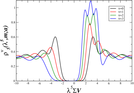
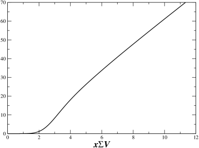
Figure 2: Left: The microscopic spectral density of $D_{5}$ for $\nu=0,1,2$ and $3$ with, $\hat{m}=3$, $\hat{a}_{8}=0.2$ and $\hat{a}_{6}=\hat{a}_{7}=0$. At nonzero value of the lattice spacing the zero modes spread out into a region around $\hat{x}=\hat{m}$. For negative values of $\nu$ the spectral density is reflected at the origin. Right: After summation over $\nu$ with a Gaussian weight and integrating from $\lambda^{5}=0$ up to $\lambda^{5}=x$. That is, the average number of eigenvalues below $x$. For the plot we have chosen $\langle\nu^{2}\rangle=1$. The values of $\hat{m}$ and $\hat{a}_{i}$ are as in the left figure. Compare with Fig. 1 of LP .

In Section II we discussed the mass dependence of $\rho_{5}^{\nu}(\lambda^{5}=0,\hat{m};\hat{a}_{i})$. The density of the real eigenvalues of $D_{W}$ satisfies the inequality (21). In Fig. 3 we plot both sides of this inequality as a function of $\lambda^{W}$.

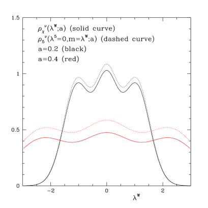
Figure 3: The distribution of the chirality over the real eigenvalues of $D_{W}$ $\rho_{\chi}^{\nu=3}(\lambda^{W};\hat{a}_{i})$ (solid curves) and $\rho_{5}^{\nu=3}(\lambda^{5}=0,\hat{m}=\lambda^{W};\hat{a}_{i})$ as a function of $\lambda^{W}$. The values of $\hat{a}_{8}$ (here denoted by $a$) are given in the legend of the Figure ($\hat{a}_{6}=\hat{a}_{7}=0$ here). The density of the real eigenvalues of $D_{W}$ is bounded between the solid and the dashed curve.

IV.3 The effect of $W_{6}$ and $W_{7}$

In the derivation above we have explicitly included the effect of $W_{6}$ and $W_{7}$ in the Lagrangian and then performed the relevant super-traces and fermionic integrations. Here we point out an alternative way to compute the effect of $W_{6}$ and $W_{7}$. Not only will this give us a direct way to quantify the effect of $W_{6}$ and $W_{7}$ on the spectrum of the Dirac operator, it also provides a simple way to include the effects of these terms in the chiral Random Matrix Theory discussed below.

Since $W_{6}$ and $W_{7}$ are coupling constants of double-trace terms, we can re-express the microscopic partition function (26) as

$$Z^{\nu}_{N_{f}}(\hat{m},\hat{z};\hat{a}_{6},\hat{a}_{7},\hat{a}_{8})=\frac{1}{16\pi\hat{a}_{6}\hat{a}_{7}}\int_{-\infty}^{\infty}dy_{6}dy_{7}\ e^{-\frac{y_{6}^{2}}{16|\hat{a}_{6}^{2}|}-\frac{y_{7}^{2}}{16|\hat{a}_{7}^{2}|}}\ Z_{N_{f}}^{\nu}(\hat{m}-y_{6},\hat{z}-y_{7};0,0,\hat{a}_{8}).$$ (48)

Here we have written the expression valid for negative values $W_{6}$ and $W_{7}$. If $W_{6}>0$ the shift of $\hat{m}$ is instead along the imaginary axis, $\hat{m}-iy_{6}$. For $W_{7}>0$ we analogously shift $\hat{z}$ along the imaginary axis, $\hat{z}-iy_{7}$.

Since exactly the same rewriting is valid for the generating function (IV) also the quenched spectral density at non-zero values of $W_{6}$ and $W_{7}$ follows from that with $W_{8}$ alone

$$\rho^{\nu}_{5}(\lambda^{5},\hat{m};\hat{a}_{6},\hat{a}_{7},\hat{a}_{8})=\frac{1}{16\pi\hat{a}_{6}\hat{a}_{7}}\int_{-\infty}^{\infty}dy_{6}dy_{7}\ e^{-\frac{y_{6}^{2}}{16|\hat{a}_{6}^{2}|}-\frac{y_{7}^{2}}{16|\hat{a}_{7}^{2}|}}\ \rho^{\nu}_{5}(\lambda^{5}-y_{7},\hat{m}-y_{6};0,0,\hat{a}_{8}).$$ (49)

Interestingly, for $W_{6}<0$ the quenched spectral density of $D_{5}$ is a Gaussian average of spectra with a smooth distribution of quark masses. The integrals over $y_{6}$ and $y_{7}$ in (48) and (49) can only be interchanged with the noncompact integral in the partition function if the inequality $\hat{a}_{8}^{2}-\hat{a}_{6}^{2}-\hat{a}_{7}^{2}>0$ is satisfied. Furthermore, the shift must be along the real axis in order that the discontinuity across the real axis remains linked to the eigenvalue density.

V Limiting Cases

In this section we discuss various limiting cases of the spectral density of $D_{5}$ and $D_{W}$. Since the Dirac spectrum at $W_{6,7}\neq 0$ is given by a Gaussian integral over the Dirac spectrum for $W_{6}=W_{7}=0$, only the dependence on $W_{8}$ will be analyzed in this section.

V.1 Small $\hat{a}_{8}$-limit for $\hat{z}-\hat{m}$ fixed

We first show explicitly that in the limit $\hat{a}_{8}\to 0$ the microscopic resolvent (IV.2) reduces to the known analytical result of the continuum limit. To derive the $\hat{a}_{8}\to 0$ limit of the microscopic spectral density, we use the integrals

$$\int_{-\pi}^{\pi}\frac{d\theta}{2\pi}e^{i\nu\theta}e^{-\hat{m}\sin\theta+i\hat{z}\cos\theta} = \left(\frac{\hat{z}-\hat{m}}{\hat{z}+\hat{m}}\right)^{\nu/2}I_{\nu}(i\,{\rm sign}(z)\sqrt{\hat{z}^{2}-\hat{m}^{2}}),$$ (50)

$$\lim_{\hat{a}_{8}\to 0}\int_{-\infty}^{\infty}dse^{-\nu s}e^{-i\hat{m}\sinh(s)-i(\hat{z}-i\epsilon)\cosh(s)-2\hat{a}_{8}^{2}\cosh(2s)}$$

$$= 2\left(\frac{\hat{z}-i\epsilon-\hat{m}}{\hat{z}-i\epsilon+\hat{m}}\right)^{-\nu/2}K_{\nu}(i\sqrt{(\hat{z}-i\epsilon)^{2}-\hat{m}^{2}}),$$

valid at fixed $|\hat{m}-\hat{z}|\neq 0$, and obtain

$$\lim_{\hat{a}_{8}\to 0}G^{\nu}(\hat{z},\hat{m};\hat{a}_{8}) = -\frac{1}{4}K_{\nu}(\eta)[(\hat{z}+\hat{m})(\beta^{2}I_{\nu+2}(\eta)+I_{\nu}(\eta))+(\hat{z}-\hat{m})(\beta^{-2}I_{\nu-2}(\eta)+I_{\nu}(\eta))]$$ (52)

$$-\frac{1}{4}[\beta I_{\nu+1}(\eta)+\beta^{-1}I_{\nu-1}(\eta)][(\hat{z}+\hat{m})\beta K_{\nu-1}(\eta)+(\hat{z}-\hat{m})\beta^{-1}K_{\nu+1}(\eta)]$$

$$+\frac{i}{2}K_{\nu}(\eta)[\beta I_{\nu+1}(\eta)+\beta^{-1}I_{\nu-1}(\eta)],$$

with

$$\eta = i\sqrt{\hat{z}^{2}-\hat{m}^{2}},\qquad\beta=\sqrt{\frac{\hat{z}-\hat{m}}{\hat{z}+\hat{m}}}.$$ (53)

We now use the recursion relations

$$I_{\nu+2}(\eta) = I_{\nu}(\eta)-\frac{2(\nu+1)}{\eta}I_{\nu+1}(\eta),$$

$$I_{\nu-2}(\eta) = I_{\nu}(\eta)+\frac{2(\nu-1)}{\eta}I_{\nu-1}(\eta),$$

$$K_{\nu+1}(\eta) = K_{\nu-1}(\eta)+\frac{2\nu}{\eta}K_{\nu}(\eta),$$ (54)

and the Wronskian identity to obtain the resolvent of $D_{5}$ in the limit $\hat{a}_{8}\to 0$ for $\hat{z}-\hat{m}$ fixed

$$G^{\nu}(\hat{z},\hat{m})=-z(I_{\nu}(\eta)K_{\nu}(\eta)+I_{\nu+1}(\eta)K_{\nu-1}(\eta))+\frac{\nu}{\hat{z}-\hat{m}}.$$ (55)

As we will now demonstrate, this is the resolvent of $D_{5}$ for $a=0$. The resolvent of $D_{W}$ at $a=0$ can be expressed as

$$\left\langle{\rm Tr}\frac{1}{D_{W}+z}\right\rangle=\left\langle\sum_{\lambda^{W}_{k}>0}\frac{2z}{(\lambda_{k}^{W})^{2}+z^{2}}\right\rangle+\frac{\nu}{z}.$$ (56)

The eigenvalues of $D_{5}$ are $\lambda_{k}^{5}=\pm\sqrt{(\lambda_{k}^{W})^{2}+m^{2}}$ for $\hat{a}_{8}=0$ resulting in the resolvent

$$\left\langle{\rm Tr}\frac{1}{D_{5}+z}\right\rangle=\left\langle\sum_{\lambda^{W}_{k}>0}\frac{2z}{z^{2}-(\lambda_{k}^{W})^{2}-m^{2}}\right\rangle+\frac{\nu}{z-m}$$ (57)

$$= -\left\langle\sum_{\lambda^{W}_{k}>0}\frac{2z}{(\lambda^{W}_{k})^{2}+m^{2}-z^{2}}\right\rangle+\frac{\nu}{z-m}$$

$$= -z\left.\frac{\Sigma^{\nu}_{\lambda^{W}_{k}>0}(x)}{x}\right|_{x=i\sqrt{z^{2}-m^{2}}}+\frac{\nu}{z-m}.$$

Inserting the $\hat{a}_{8}=0$ result for $\Sigma^{\nu}$, see eg. Eq. (45) of DOTV , we consistently find (55) above. We conclude that in the limit $\hat{a}_{8}\to 0$ the eigenvalue density $\rho_{5}^{\nu}(\lambda^{5},\hat{m};\hat{a}_{8})$ is given by the standard $\hat{a}_{8}=0$ result (43) as long as $|(\lambda^{5}-\hat{m})|/\hat{a}_{8} \gg 1$.

V.2 Small $\hat{a}_{8}$-limit for $(\hat{z}-\hat{m})/\hat{a}_{8}$ fixed

As we have just seen, for $a=0$ the contribution of the zero modes of $D_{W}$ to the resolvent of $D_{5}$ is given by

$$\frac{\nu}{\hat{z}-\hat{m}}.$$ (58)

For $a\neq 0$ the zero modes are smeared out so that the singularity in the resolvent is smoothened, and we expect the imaginary part of the resolvent to behave as

$${\rm Im}[G^{\nu}(\hat{z},\hat{m})]\sim\frac{1}{\hat{a}}_{8}F(\hat{z}-\hat{m}),$$ (59)

with $F$ a peaked function. In Appendix A we extract the analytical expression for $F$ from the small $\hat{a}_{8}$ limit of the microscopic result for the resolvent given in Eq. (IV.2). Amazingly, the result is given by the eigenvalue density of a $|\nu|\times|\nu|$ Hermitian Random Matrix Theory

$$\rho_{5}^{\nu}(\lambda^{5},\hat{m};\hat{a}_{8}\ll 1) = \frac{1}{4\hat{a}_{8}}\exp(-u^{2})\sum_{k=0}^{\nu-1}\frac{H_{k}(u)H_{k}(u)}{2^{k}k!\sqrt{\pi}}$$

$$= \frac{1}{4\hat{a}_{8}}\frac{e^{-u^{2}}}{2^{\nu}(\nu-1)!\sqrt{\pi}}[H_{\nu}^{2}(u)-H_{\nu+1}(u)H_{\nu-1}(u)],$$

with

$$u=\frac{\lambda^{5}-\hat{m}}{4\hat{a}_{8}}.$$ (61)

This is the familiar spectral density of the $\nu\times\nu$ Gaussian Unitary Ensemble shifted by $\hat{m}$ and rescaled by $1/4\hat{a}_{8}$. For $\nu=1$ the result is a simple Gaussian.

For the normalization of the Hermite polynomials we used the convention

$$\int_{-\infty}^{\infty}dx\ H_{j}(x)H_{k}(x)e^{-x^{2}}=\delta_{jk}2^{k}k!\sqrt{\pi}.$$ (62)

The $1/\hat{a}_{8}$ contribution to the spectral density is therefore normalized to $\nu$. For $\nu=0$ the leading small-$\hat{a}_{8}$ corrections are $O(\log(\hat{a}_{8}))$, see Appendix A for details, and will not be considered to the order we are working.

V.3 For small $\hat{a}_{8}$ the distribution $\rho_{\chi}^{\nu}$ is given by $\rho^{\nu}_{5}$

The distribution of the chirality over the real eigenvalues of $D_{W}$, $\rho_{\chi}^{\nu}(\lambda^{W};\hat{a}_{8})$, is obtained from the resolvent of $D_{5}$, Eq. (IV.2), by replacing the pre-exponential factor $i\cos\theta\to-\sin\theta$ and putting $z\to 0$. As discussed in section IV.1, to leading order in $\hat{a}_{8}$, this is equal the spectral density of the real eigenvalues of $D_{W}$. For small $\hat{a}_{8}$ the width of the spectrum $\sim\hat{a}_{8}$ and we can thus consider the limit of small $\hat{a}_{8}$ with $\hat{m}/\hat{a}_{8}$ fixed. This is exactly the limit that was considered in previous section.

To leading order, only the negative exponent of $-\sin\theta$ has to be taken into account (which, up to a minus sign, is the same as the negative exponent of $i\cos\theta$). We thus find

$$\rho_{\rm real}^{\nu}(\lambda^{5}-\hat{m};\hat{a}_{8})=\rho_{5}^{\nu}(\lambda^{5},\hat{m};\hat{a}_{8})\qquad{\rm for}\quad\hat{a}_{8}\to 0\quad{\rm and}\quad(\hat{m}-\lambda^{5})/\hat{a}_{8}\quad{\rm fixed}.$$ (63)

This fact is also demonstrated graphically in Figure 4. The two distributions merge because the real modes are almost chiral. To see this we start with a real mode of $D_{W}$ Itoh

$$D_{W}\phi_{j}=\lambda^{W}_{j}\phi_{j}.$$ (64)

It follows that

$$D_{5}\phi_{j}=\gamma_{5}(D_{W}+m)\phi_{j}=(\lambda^{W}_{j}+m)\gamma_{5}\phi_{j}.$$ (65)

Now if the real modes of $D_{W}$ are chiral $\gamma_{5}\phi_{j}=\pm\phi_{j}$ then the $\nu$ real eigenvalues of $D_{W}$ are mapped onto $\nu$ eigenvalues of $D_{5}$ with a trivial shift by $m$. More precisely,

$$\gamma_{5}\phi_{j}=\langle j|\gamma_{5}|j\rangle\phi_{j}+\delta\phi\qquad{\rm with}\quad\langle j|\delta\phi\rangle=0\quad{\rm and}\quad\delta\phi\sim O(a),$$ (66)

so that

$$D_{5}\phi_{j}=(m+\lambda^{W}_{j})\langle j|\gamma_{5}|j\rangle\phi_{j}+O(a).$$ (67)

Since the distributions of the two merge in the small $\hat{a}_{8}$ limit, (see Eq. (63)), this explicitly confirms that the chirality of the real modes is unity to leading order in $\hat{a}_{8}$.

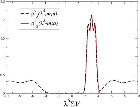
Figure 4: The microscopic spectral density of $D_{5}$ for $\nu=3$ with $\hat{m}=3$ and $\hat{a}_{8}=0.1$ and $\hat{a}_{6}=\hat{a}_{7}=0$. Also plotted is the distribution of the chirality over the real modes of $D_{W}$ shifted by the mass, that is $\rho^{\nu}_{\chi}(\lambda^{5}-\hat{m};\hat{a}_{8})$. Since the real modes are almost chiral for small $\hat{a}_{8}$ the two distributions merge.

V.4 Scaling of Smallest Eigenvalue

For $\nu=1$ and $\hat{a}_{8}\ll 1$ the distribution of the single real eigenvalue of $D_{W}$ takes the Gaussian form

$$\rho^{\nu=1}_{\rm real}(\lambda^{W};\hat{a}_{8}\ll 1)=\frac{1}{4\hat{a}_{8}\sqrt{\pi}}\exp\left(-\frac{(\lambda^{W})^{2}}{16\hat{a}_{8}^{2}}\right).$$ (68)

In physical units the width of the distribution is

$$\sigma=\frac{\sqrt{8a^{2}W_{8}}}{\Sigma\sqrt{V}}.$$ (69)

This is also the width parameter of the Gaussian tail of the spectral density of $D_{5}$ inside the gap. In lattice simulations of the Wilson Dirac operator, a scaling of the width of the distributions of the smallest eigenvalue $\sim a/\sqrt{V}$ has been reported Luscher for $N_{f}=2$ simulations.

It is also instructive to consider the ratio of the width parameter and the average spacing $\Delta\lambda=\pi/\Sigma V$ of the Dirac eigenvalues at $a=0$,

$$\frac{\sigma}{\Delta\lambda}=(8a^{2}W_{8}V)^{1/2}\frac{1}{\pi}=\hat{a}_{8}\frac{\sqrt{8}}{\pi}.$$ (70)

This gives an intuitive interpretation of the dimensionless low-energy constant $\hat{a}_{8}$.

V.5 Mean Field Limit

For large $\hat{m}$, $\hat{z}$, and $\hat{a}_{i}^{2}$ the graded generating function can be evaluated by a saddle point approximation. This limit corresponds to the lowest non-trivial order in the usual perturbative expansion ($p$-regime) as considered in Sharpe2006 . We will focus, in particular, on the behavior of the spectral density $\rho_{5}$ near the edge of the spectrum. At mean field level the dependence on the index of the Dirac operator is suppressed and we will therefore start from the $\nu=0$ expression and drop the index $\nu$ below. Since the Dirac spectrum at $W_{6,7}\neq 0$ is given by a Gaussian integral over the Dirac spectrum for $W_{6}=W_{7}=0$, only the dependence on $W_{8}$ will be taken into account in this section.

The expression for the spectral density can be written as

$$\rho_{5}^{\nu=0}(\hat{m},\hat{z};\hat{a}_{8})=\frac{1}{\pi}{\rm Im}\int_{-\infty}^{\infty}ds\int_{-\pi}^{\pi}\frac{d\theta}{2\pi}e^{S_{f}(\hat{m},\hat{z};\hat{a}_{8})}\frac{d}{dz^{\prime}}e^{S_{b}(\hat{m},\hat{z}^{\prime};\hat{a}_{8})}P(\hat{m},\hat{z},\hat{z}^{\prime};\hat{a}_{8})\big{|}_{\hat{z}^{\prime}=\hat{z}},$$ (71)

where $S_{f}$, $S_{b}$ and $P$ can be read off from Eqs. (45), (IV.2). By shifting integration contours according to

$$\theta = i(-r+\frac{i\pi}{2}),$$

$$s = t-\frac{\pi i}{2},$$ (72)

the fermionic and bosonic exponents become real and equal up to a sign

$$\tilde{S}_{f}(r) = \hat{m}\cosh r+\hat{z}\sinh r-2\hat{a}_{8}^{2}\cosh 2r,$$

$$\tilde{S}_{b}(t) = -\hat{m}\cosh t-\hat{z}\sinh t+2\hat{a}_{8}^{2}\cosh 2t.$$ (73)

Also the prefactor in terms of these variables

$$P(s,r)=-\frac{i}{2}[\hat{m}\cosh r+\hat{z}\sinh r+\hat{m}\cosh t+\hat{z}\sinh t-2\hat{a}_{8}^{2}((e^{r}+e^{t})^{2}+(e^{-r}+e^{-t})^{2})]$$ (74)

becomes real (an overall factor of $i$ is included in the fermionic integration).

For large $\hat{m}$ and $\hat{z}$ the integrals can be evaluated by a saddle point approximation. It is convenient to introduce $u=\sinh s$ as new variable so that the potential (73) is given by

$$S_{b}(u)=-\hat{m}\sqrt{1+u^{2}}-\hat{z}u+2\hat{a}_{8}^{2}(2u^{2}+1).$$ (75)

The edge of the spectrum is the point where two real saddle points coalesce and move into the complex plane. At this point

$$S^{\prime}_{b}(u_{g})=0,\qquad{\rm and}\qquad S_{b}^{\prime\prime}(u_{g})=0,$$ (76)

where $S_{b}(u)$ ia given in Eq. (75). The second equation results into

$$u_{g}^{2}=\left(\frac{\hat{m}}{8\hat{a}_{8}^{2}}\right)^{2/3}-1,$$ (77)

which combined with the vanishing first derivative leads to the mean field result for the gap

$$\hat{z}_{g}=\hat{m}\left(1-\left(\frac{8\hat{a}_{8}^{2}}{\hat{m}}\right)^{2/3}\right)^{3/2}.$$ (78)

The mean field spectrum is symmetric around the origin and above we displayed the positive solution for the gap.

Depending on the position of $\lambda^{5}$ with respect to the position of the gap $\hat{z}_{g}$ we can distinguish three parameter domains:

• $|\lambda^{5}|<z_{g}$, then all saddle points in terms of the $r$ and $t$ variables are real. The leading saddle point determines the fermionic integral but does not contribute to the imaginary part of the bosonic integral (which gives the imaginary part of the resolvent). The imaginary part is given by a subleading saddle point when combined with the fermionic contribution gives an exponentially suppressed tail. Combining this with the fermionic integral gives the spectral density. In the small $\hat{a}_{8}$ limit, when $\cosh s\approx\sinh s$ at the saddle point, the bosonic integral becomes Gaussian resulting in the Gaussian tail

  $$\rho_{5}(\lambda^{5},\hat{m};\hat{a}_{8})\sim\exp\left(\hat{m}-\frac{\hat{m}^{2}}{2(\hat{m}-8\hat{a}_{8}^{2})}-\frac{(\hat{m}-\lambda^{5})^{2}}{16\hat{a}_{8}^{2}}\right).$$ (79)

• $|\lambda^{5}|>z_{g}$, then a pair of real saddle points has turned into a pair of complex conjugate saddle points. Only one of the saddle points can be accessed by the bosonic integration contour, but they both contribute to the fermionic integral. When the saddle points of the bosonic and fermionic integrals are the same, the exponents cancel resulting in a smooth contribution to the spectral density. When they are different, they result in an oscillatory exponent which is subleading because of the prefactor. It is instructive to work out the case $\hat{a}_{8}=0$ which is done in Appendix B. Also the non-zero $\hat{a}_{8}$ case is discussed in this appendix.

• $\lambda^{5}\approx z_{g}$, then two saddle points are close and the exponents can be approximated by a cubic polynomial. This is the scaling domain where $V(z-z_{g})^{3/2}$ is kept fixed in the thermodynamic limit for fixed $m$ and $a$. In principle, the exact generating function can be evaluated in this limit, and according to universality arguments it should give a spectral density that can be expressed in terms of Airy functions as (see Eq. (153) for the definition of $\Delta$)

  $$\rho_{5}(x)=\frac{1}{\Delta}({\rm Ai}^{\prime}(x)^{2}-x{\rm Ai}^{2}(x)),\qquad{\rm with}\qquad x=(z_{g}-z)/\Delta.$$ (80)

  The leading order asymptotic behavior of the Airy function on both sides of $z_{g}$ follows from a saddle point approximation of the generating function in this domain. This is shown in Appendix B.

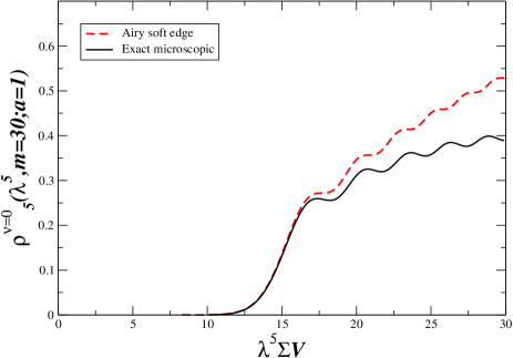
Figure 5: The Airy behavior of $\rho_{5}^{\nu}(\lambda^{5},\hat{z})$ dots for $\hat{m}=30$, $\hat{a}_{8}=1$ and $\lambda^{5}$ close to $z_{g}$ vs. Eq. (80).

V.6 Edge Scaling

As discussed in previous section, the supersymmetric generating function can be evaluated in a counting scheme where $\hat{m}\gg 1$, $\hat{a}_{8}^{2}\gg 1$ and $(\hat{z}-\hat{z}_{g})^{3/2}\gg 1$ are all of the same order. This is a universal scaling domain where the average spectral density is given by the expression in terms of Airy functions (see Eq. (80)). We illustrate this in Fig. 5 for $\hat{m}=30$ and $\hat{a}_{8}=1$.

The distribution, $p_{\rm min}$, of the smallest positive eigenvalue for the corresponding density Eq. (80) is also known. It is given by the Tracy-Widom distribution Tracy ; For ; NWch6 for $\beta=2$,

$$p_{\rm min}(z)=\frac{d}{dz}F_{2}((z-z_{g})/\Delta),$$ (81)

$$F_{2}(x)=e^{-\int_{-\infty}^{x}(x-y)q^{2}(y)dy},$$ (82)

where $q(x)$ is the solution of

$$q^{\prime\prime}(x)=-xq(x)+2q^{3}(x)$$ (83)

with boundary condition that $q(x)\to{\rm Ai}(-x)$ for $x\to-\infty$.

VI Random Matrix Theory for the Wilson Dirac Operator

A chiral Random Matrix Theory for lattice QCD with Wilson fermions is constructed from the most general $\gamma_{5}$-Hermitian matrix. This random matrix Wilson Dirac operator has the block structure

$$\tilde{D}_{W}=\left(\begin{array}[]{cc}\tilde{a}A&iW\\ iW^{\dagger}&\tilde{a}B\end{array}\right),$$ (86)

where

$$A=A^{\dagger}\quad{\rm and}\quad B^{\dagger}=B$$ (87)

are $(n+\nu)\times(n+\nu)$ and $n\times n$ complex matrices, respectively, and $W$ is an arbitrary complex $(n+\nu)\times n$ matrix. In Eq. (86) and below we use tildes to indicate quantities in the Random Matrix Theory which are analogues of those in the quantum field theory. We relate the two sets in Eq. (94).

We take the matrix elements to be distributed with Gaussian weight

$${\cal P}(A,B,W)\equiv e^{-\frac{N}{4}{\rm Tr}[A^{2}+B^{2}]-\frac{N}{2}{\rm Tr}[WW^{\dagger}]},$$ (88)

where $N=2n+\nu$. Because of universality, results in the microscopic domain should not depend on the details of the probability distribution RMT2 , but for simplicity we take a Gaussian distribution. The partition function of the Wilson chiral Random Matrix Theory is then defined as

$$\tilde{Z}^{\nu}_{N_{f}}=\int dAdBdW\ \prod_{f=1}^{N_{f}}\det(\tilde{D}_{W}+\tilde{m}_{f}+\tilde{z}_{f}\tilde{\gamma}_{5})\ {\cal P}(A,B,W).$$ (89)

The matrix integrals are over the complex Haar measure and $\tilde{\gamma}_{5}={\rm diag}(1,\cdots,1,-1,\cdots,-1)$ is a diagonal matrix with $n+\nu$ diagonal matrix elements equal to 1 and $n$ diagonal matrix elements equal to $-1$.

For large quark mass the matrix $\tilde{D}_{5}\equiv\gamma_{5}(\tilde{D}_{W}+m)$ has $n+\nu$ positive eigenvalues and $n$ negative eigenvalues, whereas for large negative mass $\tilde{D}_{5}$ has $n+\nu$ negative eigenvalues and $n$ positive eigenvalues. Therefore at least $|\nu|$ spectral flow curves of $\tilde{D}_{5}$ have to cross zero at least once. Since each crossing corresponds to a real eigenvalue of $\tilde{D}_{W}$ we conclude that $\tilde{D}_{W}$ has at least $|\nu|$ real eigenvalues. The block structure of the matrix (86) guarantees that the Random Matrix Dirac operator has index $\nu$.

A chiral Random Matrix Theory for staggered fermions at finite lattice spacings was introduced in James .

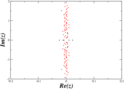
Figure 6: Scatter plot of the eigenvalues of $\tilde{D}_{W}$ with $\nu=5$ as obtained from Wilson chiral Random Matrix Theory. The real eigenmodes (black dots) are clearly visible. The width of the strip of complex eigenvalues in the thermodynamic limit equals $|{\rm Re}(z)|<8a^{2}W_{8}/\Sigma$, as also follows from the chiral Lagrangian. See Eq. (94) for the match between the parametrs of Wilson chiral Random Matrix Theory and those of the chiral Lagrangian.

VI.1 From Wilson chiral Random Matrix Theory to Wilson chiral Perturbation Theory

We now consider the microscopic limit of the chiral Random Matrix Theory for Wilson fermions in which

$$\tilde{m}\sim N^{-1},\qquad\tilde{z}\sim N^{-1},\qquad\tilde{a}\sim N^{-1/2}.$$ (90)

We have studied numerically the quenched eigenvalue spectrum of the random matrix Wilson Dirac operator, $\tilde{D}_{W}$, in this scaling regime. We find that the number of real eigenvalues of $\tilde{D}_{W}$ is equal to $\nu+O(\tilde{a}^{4})$ for $\nu\neq 0$ and $\nu+O(\tilde{a}^{2})$ for $\nu=0$, while the remaining eigenvalues come in complex conjugate pairs, see Fig. 6. Moreover, we have found perfect agreement with the analytical predictions for $\rho_{\chi}^{\nu}$ in Eq. (41) and $\rho^{\nu}_{5}$ in Eq. (47), this is illustrated by Fig. 7. This agreement strongly suggest that the chiral Random Matrix Theory for Wilson fermions introduced above is in the same spectral universality class as the leading term of Wilson chiral Perturbation Theory in the $\epsilon$-counting scheme.

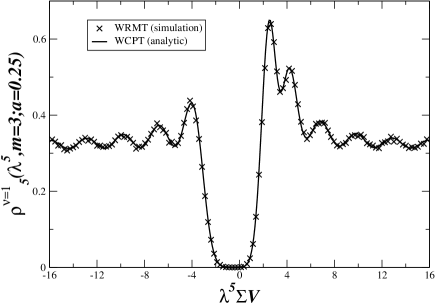
Figure 7: The average spectral density of the hermitian Random Matrix Dirac operator $\tilde{D}_{5}$ with $n=50$ and $\nu=1$ over an ensemble of 100,000 matrices (marked by crosses) and the prediction from Wilson Chiral Perturbation Theory.

To demonstrate this universality we will now show that the Wilson chiral Random Matrix Theory partition function reduces to that of Wilson chiral Perturbation Theory to leading order in the $\epsilon$-counting scheme. The explicit calculation will allow us to identify the low energy constant $W_{8}$ in terms of the parameters of the Random Matrix Theory. Inclusion in the Random Matrix Theory of the two other terms in the chiral Lagrangian to this order that couple with $W_{6}$ and $W_{7}$ will be discussed in the next subsection. For notational simplicity we keep the quark flavors degenerate.

The first step is to express the determinants in Eq. (89) as Grassmann integrals. Then the average over the matrix elements of $W$ can be performed by completing squares, see SV ; RMT1 for details. The four-fermion terms can be decoupled by means of a Hubbard-Stratonovitch transformation, leading to the partition function

$$\tilde{Z}^{\nu}_{N_{f}}(\tilde{m},\tilde{z};\tilde{a}) = \int dQ_{1}dQ_{2}dTdT^{\dagger}$$

$$\times{\det}^{N/2+\nu}(i\tilde{a}Q_{1}+T+\tilde{m}+\tilde{z}){\det}^{N/2}(i\tilde{a}Q_{2}+T^{\dagger}+\tilde{m}-\tilde{z})e^{-\frac{N}{2}{\rm Tr}TT^{\dagger}-\frac{N}{4}{\rm Tr}[Q_{1}^{2}+Q_{2}^{2}]}.$$

Here, $Q_{1}$ and $Q_{2}$ are Hermitian $N_{f}\times N_{f}$ matrices and $T$ is an arbitrary complex $N_{f}\times N_{f}$ matrix.

Up to now this is an exact reformulation of the partition function (89). In the limit of large matrices valid for the scaling (90) the integrals can be evaluated by a saddle point approximation. The saddle point manifold is given by

$$T=UV^{-1}.$$ (92)

After absorbing $V^{-1}$ in $U$ and expanding the exponent to order $\tilde{m}$, $\tilde{z}$ and $\tilde{a}^{2}$ we obtain

$${\tilde{Z}}^{\nu}_{N_{f}}(\tilde{m},\tilde{z};\tilde{a}) = \int_{U(N_{f})}dU\int dQ_{1}dQ_{2}\ {\det}^{\nu}(U)\ e^{\frac{N}{2}(\tilde{m}+\tilde{z}){\rm Tr}U+\frac{N}{2}(\tilde{m}-\tilde{z}){\rm Tr}U^{\dagger}}$$

$$\times e^{\frac{N}{2}i\tilde{a}{\rm Tr}(Q_{1}U+Q_{2}U^{-1})+\frac{N}{4}\tilde{a}^{2}{\rm Tr}[Q_{1}U^{-1}Q_{1}U^{-1}+Q_{2}UQ_{2}U]-\frac{N}{4}{\rm Tr}(Q_{1}^{2}+Q_{2}^{2})}.$$

The integrals over $Q_{1}$ and $Q_{2}$ are Gaussian and are localized on the saddle point. The term of $O(\tilde{a}^{2})$ in the exponent results in higher order contributions and they can be omitted here. We thus obtain the partition function

$$\tilde{Z}^{\nu}_{N_{f}}(\tilde{m},\tilde{z};\tilde{a})=\int_{U(N_{f})}dU\ {\det}^{\nu}(U)\ e^{\frac{N}{2}(\tilde{m}+\tilde{z}){\rm Tr}U+\frac{N}{2}(\tilde{m}-\tilde{z}){\rm Tr}U^{\dagger}-N\frac{\tilde{a}^{2}}{4}{\rm Tr}(U^{2}+{U^{\dagger}}^{2}).}$$ (93)

This shows that the Wilson chiral Random Matrix Theory partition function (VI.1) reproduces the three leading terms in the $\epsilon$-expansion. The corresponding low energy constants are identified as

$$N\tilde{m}={m\Sigma V},\quad N\tilde{z}={z\Sigma V},\quad\frac{N\tilde{a}^{2}}{4}=a^{2}W_{8}V.$$ (94)

As discussed in section VII.3 this identification requires that $W_{8}>0$.

VI.2 Double-Trace terms

The double-trace terms of Wilson chiral Perturbation Theory are not generated by the Wilson Random Matrix Theory defined in Eq. (89). Although such terms have been argued to be suppressed in large-$N_{c}$ counting KL , we would nevertheless like to be able to include them. As we will now show, this can easily be done.

Let the Random Matrix Theory partition function be extended to

$$\tilde{Z}^{\nu}_{N_{f}}(\tilde{m},\tilde{z};\tilde{a}_{6},\tilde{a}_{7},\tilde{a}_{8})\equiv\frac{1}{16\pi\tilde{a}_{6}\tilde{a}_{7}}\int_{-\infty}^{\infty}dy_{6}dy_{7}\ e^{-\frac{y_{6}^{2}}{16|\tilde{a}_{6}^{2}|}-\frac{y_{7}^{2}}{16|\tilde{a}_{7}^{2}|}}\ \tilde{Z}_{N_{f}}^{\nu}(\tilde{m}-y_{6},\tilde{z}-y_{7};\tilde{a}_{8}),$$ (95)

where the partition function inside the integral is given in (89). It follows from the discussion of subsection IV.3 that then also the trace-squared terms of Wilson chiral Perturbation Theory are reproduced by the Random Matrix Theory in the scaling limit (90). The partition functions (95) lead to negative values of $W_{6}$ and $W_{7}$. Positive values of these constants can be obtained from fluctuations of the mass in the imaginary direction.

VII Hermiticity Properties and the Sign of $W_{8}$

The sign and magnitude of the low energy constants $W_{6}$, $W_{7}$ and $W_{8}$ are essential for numerical simulations of lattice QCD with Wilson fermions. In particular the sign of $W_{8}$ has been debated in the literature Sharpe2006 ; Azcoiti:2008dn ; Shindler:2009ri . The sign is important for understanding whether or not lattice QCD with Wilson fermions enters an Aoki phase with spontaneously broken parity Aokiclassic ; Heller . In this section we provide several arguments for why Hermiticity properties put constraints on the these low-energy parameters. To simplify the discussion, we restrict ourselves to the case where both $W_{6}$ and $W_{7}$ vanish.

VII.1 A Wilson lattice QCD inequality and the sign of $W_{8}$

With two degenerate flavors the determinant of the Wilson Dirac operator is positive definite and it is possible to formulate rigorous QCD inequalities. Based on such an inequality we argue here that for $W_{6}=W_{7}=0$ one must have $W_{8}\geq 0$ in the $N_{f}=2$ theory. Since the Wilson fermion determinant in lattice QCD is real, the measure with two degenerate flavors is real and positive

$${\det}^{2}(D_{W}+m)>0.$$ (96)

As this is true for any gauge field configuration, independent of the number of real eigenvalues of $D_{W}$, it follows that the two-flavor partition function, ${\cal Z}^{\nu}_{N_{f}=2}$, of lattice QCD with Wilson fermions in a sector with fixed number of real modes of $D_{W}$ is real and positive for all real values of $m$

$${\cal Z}^{\nu}_{N_{f}=2}(m,z=0;a)>0.$$ (97)

The overall sign of the partition function can of course be changed by introducing a multiplicative constant. What the inequality states is that the partition function cannot change sign as a function of a real valued quark mass.

The partition function in the $\epsilon$-regime must necessarily satisfy the same positivity bound. We note, however, that its sign depends on the index $\nu$ of the chiral Lagrangian:

$$Z_{N_{f}=2}^{\nu}(\hat{m},\hat{z};-\hat{a}_{8}^{2})=(-1)^{\nu}Z_{N_{f}=2}^{\nu}(i\hat{z},i\hat{m};\hat{a}_{8}^{2}).$$ (98)

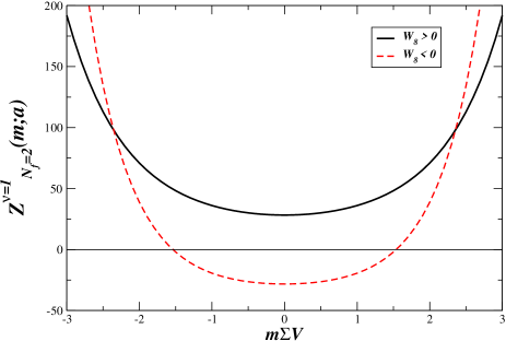
Figure 8: The two flavor microscopic partition function for $\hat{a}_{8}^{2}=1$ ($W_{8}\geq 0$) and $\hat{a}_{8}^{2}=-1$ ($W_{8}\leq 0$) plotted as a function of the mass for $\hat{z}=0$. Only the partition function with $W_{8}\geq 0$ satisfies the QCD inequality.

For odd $\nu$ the partition functions with positive and negative $\hat{a}_{8}^{2}$ have opposite signs at $m=z=0$ and, since for sufficiently large $\hat{m}$ both partition functions have the same sign, it is not possible that they both satisfy the inequality for real $\hat{m}$ and $\hat{z}$. As the plot in Fig. 8 demonstrates, the sign of $W_{8}$ dictated by the inequality is positive.

This can also can be obtained analytically from the chiral Lagrangian. The partition function with degenerate masses (III) can be expressed in terms of the eigenvalues of $U$. This allows us to rewrite the mass-degenerate partition function in the simplified form

$$Z_{N_{f}}^{\nu}(\hat{m},\hat{z};\hat{a}_{8}) = \det[Z^{\nu+i-j}_{N_{f}=1}(\hat{m},\hat{z};\hat{a}_{8})]_{i,j=1\ldots N_{f}}$$ (99)

where the one flavor partition function is

$$Z_{N_{f}=1}^{\nu}(\hat{m},\hat{z};\hat{a}_{8}) = \int_{-\pi}^{\pi}\frac{d\theta}{2\pi}\ e^{i\theta\nu}e^{\hat{m}\cos(\theta)+i\hat{z}\sin(\theta)-2\hat{a}_{8}^{2}\cos(2\theta)}.$$ (100)

In Appendix C we show that for odd values of $\nu$ the two-flavor partition function with $W_{8}>0$ ($W_{8}<0$) is positive (negative) for $\hat{m}=0$ and that for both signs of $W_{8}$ the curvature at zero mass is positive.

Below we discuss the sign of $W_{8}$ from the perspective of the graded generating function and from Wilson chiral Random Matrix Theory. In both instances we find $W_{8}\geq 0$, independent of the number of flavors.

VII.2 Convergence and $\gamma_{5}$-Hermiticity

The issue of the sign of the constants of Wilson chiral Perturbation Theory manifests itself also in the convergence properties of the graded generating functional. For $W_{6}=W_{7}=0$ the integrals in (IV) are divergent if $W_{8}<0$. However, the alternative graded generating function

$$Z_{1|1}^{\nu}({\cal M},{\cal Z};\hat{a}_{8}^{2}<0)=\int dU\ {\rm Sdet}(U)^{\nu}\ e^{\frac{1}{2}{{\rm STr}}({\cal M}[U+U^{-1}])+\frac{1}{2}{{\rm STr}}({\cal Z}[U-U^{-1}])-\hat{a}_{8}^{2}{{{\rm STr}}(U^{2}+U^{-2})}}$$ (101)

is now convergent. This integral seems to provide a bona fide generating function for Wilson fermions with $W_{8}<0$. In fact, it agrees precisely with the generating function suggested for $p$-regime calculations in ref. Sharpe2006 . Nevertheless, the sign-issue has not disappeared, it has only resurfaced in disguise. To see this, we can compute the resolvent for the real eigenvalues of $D_{W}$ with the alternative graded generating function

$$\left.\frac{d}{dm}Z_{1|1}^{\nu}({\cal M},{\cal Z}=0;\hat{a}_{8}^{2}<0)\right|_{m^{\prime}=m}.$$ (102)

By comparison with Eqs. (IV) and (101), it follows that

$$\left.\frac{d}{dm}Z_{1|1}^{\nu}({\cal M},{\cal Z}=0;\hat{a}_{8}^{2}<0)\right|_{m^{\prime}=m}=-i\left.\frac{d}{dz}Z_{1|1}^{\nu}({\cal M}=0,{\cal Z};\hat{a}_{8}^{2}>0)\right|_{z^{\prime}=z=im}.$$ (103)

Since the rhs is continuous when $m$ crosses the real axis we conclude that for $W_{8}<0$ the density of real eigenvalues vanishes. This is because the graded partition function, (101), valid for $W_{8}<0$, is the generating functional of an anti-Hermitian operator with a spectral density on the imaginary axis. This would be an acceptable eigenvalue density if $D_{W}$ was anti-Hermitian, but this is only the case for $a=0$. Away from $a=0$ the operator is only $\gamma_{5}$-Hermitian. So from the convergence of the graded generating function and the requirement of $\gamma_{5}$-Hermiticity of $D_{W}$ it follows that $W_{8}>0$.

The possibility of a link between the integration domain of the graded generating functional in chiral Perturbation Theory and the Hermiticity properties of the Dirac operator is not new. In continuum QCD at non-zero quark chemical potential the Dirac operator is non-Hermitian for real values of the chemical potential and anti-Hermitian for imaginary values. Correspondingly, the graded generating functional has two branches which differ by a transformation of the super Goldstone field Factorization ; Bosonic . One is convergent for real values of the chemical potential while the other is convergent for imaginary values of the chemical potential Fpi1 ; Fpi2 .

VII.3 The sign of $W_{8}$ and Wilson chiral Random Matrix Theory

In this section we discuss the constraints on the constants in Wilson chiral Perturbation Theory due to $\gamma_{5}$-Hermiticity from the point of view of chiral Random Matrix Theory.

In Eq. (94) the coefficients of Wilson chiral Perturbation Theory where expressed in terms of the parameters of the chiral Random Matrix Theory, and it was found that $W_{8}>0$. A chiral Random Matrix Theory where the sign of $W_{8}$ is negative can be obtained by including an additional imaginary unit $i$ in front of the chiral symmetry violating pieces of $\tilde{D}_{W}$ in (86), that is

$$\tilde{D}_{W_{8}<0}=\left(\begin{array}[]{cc}iaA&iW\\ iW^{\dagger}&iaB\end{array}\right).$$ (106)

With this change, the Random Matrix Wilson Dirac operator, however, becomes anti-Hermitian rather than $\gamma_{5}$-Hermitian. We stress that this observation is in perfect agreement with the conclusion obtained from the convergence requirement of the graded generating function above: the spectral density of the anti-Hermitian Random Matrix (106) matches that generated by the graded partition function (101) which is convergent for $W_{8}<0$. This has been verified numerically to high accuracy. Because $\tilde{D}_{W_{8}<0}$ is anti-Hermitian, the determinant $\det(\tilde{D}_{W_{8}<0}+m)^{2}$ has a definite sign for imaginary $m$ in agreement with the chiral Lagrangian for $W_{8}<0$ and imaginary $m$.

From the point of view of Random Matrix Theory, the different universality classes corresponding to whether one imposes $\gamma_{5}$-Hermiticity or not are well understood Magnea . In the Random Matrix Theory literature this is referred to as $Q$-symmetry.

Clearly the conclusions of this section have the same origin, namely that the case $W_{8}<0$ (and $W_{6}=W_{7}=0$) is in conflict with the $\gamma_{5}$-Hermiticity of $D_{W}$ and the Hermiticity of $D_{5}$. A positive sign of $W_{8}$ is consistent with the existence of an Aoki phase.

VIII Conclusions

In this paper we analyzed the spectral properties of the Wilson Dirac operator in the microscopic scaling regime. Eigenvalues of the Wilson Dirac operator in this regime are responsible for spontaneous chiral symmetry breaking. Another feature of Wilson fermions is the existence of the Aoki phase with spontaneous breaking of parity. In the microscopic scaling regime one has analytical means for studying both. We have shown that the chiral Lagrangian for Wilson Chiral Perturbation Theory can be used to compute spectral properties of the Wilson Dirac operator $D_{W}$ and its Hermitian counterpart $D_{5}$. Using a graded extension of the chiral Lagrangian up to and including ${\cal O}(a^{2})$ effects, we have computed the microscopic spectrum of the Hermitian Wilson Dirac operator $D_{5}$ in the quenched theory. We have shown how to incorporate all possible terms of the Lagrangian to this order, including double trace terms.

An alternative path to the microscopic spectrum goes through a chiral Random Matrix Theory based on symmetries of the Wilson Dirac operator. Here we have formulated such a theory and proved that the partition function coincides with that of Wilson chiral Perturbation Theory to leading order in the $\epsilon$ counting scheme. Numerically, we have demonstrated that also the spectral correlation functions of the chiral Random Matrix Theory agree beautifully with the analytical predictions of Wilson chiral Perturbation Theory.

Interestingly, we find restrictions on the possible values of the low-energy constants of Wilson Chiral Perturbation Theory arising from the imposition of $\gamma_{5}$ Hermiticity. It would be most interesting to have a more detailed understanding of this phenomenon, which seems to run deep. It is noteworthy that the bound we get from the chiral Lagrangian matches exactly with the bound we get, by an entirely different route, from our Wilson chiral Random Matrix Theory. In its simplest form, where we ignore double trace terms, it was found that this bound is consistent with the existence of an Aoki phase.

The results presented here are are for the microscopic limit in sectors with a fixed index of the Wilson Dirac operator. The real modes of the Wilson Dirac operator have an interesting dynamics on their own. Remarkably, we find that very close to the continuum, the $|\nu|$ real modes behave like the eigenvalues of a $|\nu|\times|\nu|$ Hermitian Random Matrix Theory of exactly Gaussian weight. We emphasize that this is a universal result that has been derived from a chiral Lagrangian. In lattice gauge theory simulations it would be most interesting to study just this subset of real modes of the Wilson Dirac operator. In particular, as we have shown, their dynamics carries detailed information about the low-energy constants of Wilson Chiral Perturbation Theory.

In general, we suggest to use spectral properties of the Wilson Dirac operator to determine the new parameters of Wilson Chiral Perturbation Theory. While these parameters are unphysical, it is nevertheless crucial to establish their values if one wishes to extract physical observables from Wilson fermion simulations at finite lattice spacings. It will thus be of obvious interest to extend the first results presented here for the quenched theory to the corresponding theories with $N_{f}$ light fermions. Work in this direction is presently underway latNf1 .

Acknowledgments: We would like to thank many participants of the Lattice 2010 Symposium and the TH-Institute “Future directions in lattice gauge theory - LGT10” at CERN for discussions. We thank C. Gattringer for clarifying correspondence. Two of us (GA and JV) would like to thank the Niels Bohr Foundation for support and the Niels Bohr Institute and the Niels Bohr International Academy for its warm hospitality. This work was supported by U.S. DOE Grant No. DE-FG-88ER40388 (JV) and the Danish Natural Science Research Council (KS).

Appendix A Small $\hat{a}_{8}$-Limit of Resolvent for $(\hat{z}-\hat{m})/\hat{a}_{8}$ Fixed.

In this appendix we consider the leading nontrivial expansion of $\rho_{5}^{\nu}$ for small $\hat{a}_{8}$ at $\nu\geq 0$. We start from (IV.2) with $W_{6}=W_{7}=0$ and then compute the small $\hat{a}_{8}$ limit for $(\hat{z}-\hat{m})/\hat{a}_{8}$ fixed. Our aim is to prove that in this limit the eigenvalue density is given by the familiar expression for the density of the Gaussian Unitary Ensemble with matrices of size $\nu\times\nu$.

The fermionic $\theta$-integrals in (IV.2) are all of the form

$$Z_{p}^{f} \equiv \frac{1}{2\pi}\int_{-\pi}^{\pi}d\theta e^{ip\theta}e^{-\hat{m}\sin\theta+i\hat{z}\cos\theta+2\hat{a}_{8}^{2}\cos 2\theta},\ \ \ \mbox{for}\ \ p=\nu-3,\ldots,\nu+3$$ (107)

$$= \frac{1}{2\pi}\int_{-\pi}^{\pi}d\theta e^{ip\theta}e^{\sqrt{\hat{m}^{2}-\hat{z}^{2}}\cos(\theta+\phi)+2\hat{a}_{8}^{2}\cos 2\theta}$$

$$= \frac{1}{2\pi}\int_{-\pi}^{\pi}d\theta e^{ip(\theta-\phi)}e^{\sqrt{\hat{m}^{2}-\hat{z}^{2}}\cos(\theta)+2\hat{a}_{8}^{2}\cos 2(\theta-\phi)},$$

with

$$e^{-i\phi}=\left(\frac{\hat{z}-\hat{m}}{\hat{z}+\hat{m}}\right)^{1/2}\qquad{\rm and}\qquad\cos\phi=\frac{i\hat{z}}{\sqrt{\hat{m}^{2}-\hat{z}^{2}}},\qquad\sin\phi=\frac{\hat{m}}{\sqrt{\hat{m}^{2}-\hat{z}^{2}}}.$$ (108)

To obtain the small $\hat{a}_{8}$ and small $\hat{m}-\hat{z}$ limit we expand the exponential functions in a Taylor series

$$Z_{p}^{f} = \frac{1}{2\pi}\int_{-\pi}^{\pi}d\theta e^{ip(\theta-\phi)}\sum_{k,l=0}^{\infty}\frac{1}{k!l!}(\hat{m}^{2}-\hat{z}^{2})^{k/2}\cos^{k}\theta(2\hat{a}_{8}^{2}\cos 2(\theta-\phi))^{l}.$$ (109)

The leading terms, which we will refer to as $\check{Z}_{p}^{f}$, are obtained from exponents in the cosines with opposite sign to the sign of $p$

$$\check{Z}_{p}^{f} \equiv e^{-ip\phi}{\sum_{k+2l=|p|}}\frac{1}{k!l!2^{k}}(\hat{m}^{2}-\hat{z}^{2})^{k/2}\hat{a}_{8}^{2l}e^{2il\,{\rm sign}(p)\phi}$$ (110)

$$= {\sum_{k+2l=|p|}}\frac{1}{k!l!2^{k}}(\hat{m}^{2}-\hat{z}^{2})^{k/2}\hat{a}_{8}^{2l}e^{-ik\,{\rm sign}(p)\phi}$$

$$= (\hat{a}_{8}\sqrt{2})^{|p|}{\sum_{l=0}^{[|p|/2]}}\frac{\alpha^{|p|-2l}}{(|p|-2l)!l!2^{l}},$$

where we define

$$\alpha=\frac{i(\hat{z}-{\rm sign}(p)\hat{m})}{2\hat{a}_{8}\sqrt{2}}.$$ (111)

For $p=0$ we have $\check{Z}_{p=0}^{f}=1$. The sum above can be expressed in terms of Hermite polynomials, normalized according to (62), for all $p$,

$$\check{Z}_{p}^{f}=(\hat{a}_{8}\sqrt{2})^{|p|}\frac{i^{|p|}}{2^{|p|/2}\ |p|!}H_{|p|}(\alpha/(i\sqrt{2})),$$ (112)

where the only dependence on the sign of $p$ is in the argument $\alpha$ (noting that $H_{0}=1$).

We now turn to the bosonic $s$-integrals in (IV.2). They are all of the form

$$Z_{p}^{b} \equiv \int_{-\infty}^{\infty}ds\ e^{-ps}e^{-i\hat{m}\sinh(s)-i\hat{z}\cosh(s)-2\hat{a}_{8}^{2}\cosh(2s)}\ ,\ \ \ \mbox{for}\ \ p=\nu-2,\ldots,\nu+2\ ,$$ (113)

$$= \int_{0}^{\infty}\frac{dy}{y}\ y^{-p}e^{-\frac{i}{2}(\hat{m}+\hat{z})y-\frac{i}{2}(\hat{z}-\hat{m})/y-\hat{a}_{8}^{2}(y^{2}+y^{-2})},$$

after using the same definition as in (108) and changing variables $y=e^{s}$. In the limit $a\to 0$ with $|\hat{m}-\hat{z}|/\hat{a}_{8}$ fixed the leading contribution in an expansion in powers of $\hat{a}_{8}$ is given as follows.

For $p>0$ ($p<0$) we change to rescaled new variables $y=\hat{a}_{8}\sqrt{2}/t$ ($y=t/\hat{a}_{8}\sqrt{2}$) to obtain to leading order

$$\check{Z}_{p}^{b} \equiv (\hat{a}_{8}\sqrt{2})^{-|p|}\int_{0}^{\infty}dt\ t^{|p|-1}\exp[-\alpha t-t^{2}/2]$$ (114)

$$= (|p|-1)!D_{-|p|}(\alpha)\frac{e^{\alpha^{2}/4}}{(\hat{a}_{8}\sqrt{2})^{|p|}},$$

with $D_{p}$ a parabolic cylinder function Abramowitz , and $\alpha$ depending on sign$(p)$ defined in (111).

For $p=0$ the behavior in $\hat{a}_{8}$ is different. Because of the exact result $Z_{p}^{b}(\hat{z}=0=\hat{m})=K_{0}(2\hat{a}_{8}^{2})$ we expect a logarithmic singularity here. Splitting the integration in Eq. (113) into $(0,1)$ and $(1,\infty)$ and changing variables as for $p>0$ for the former integral, and as for $p<0$ for the latter, we arrive at

$$Z_{p=0}^{b} = \int_{\hat{a}_{8}\sqrt{2}}^{\infty}\frac{dt}{t}\left[e^{-\frac{i}{2}(\hat{m}+\hat{z})\frac{\hat{a}_{8}\sqrt{2}}{t}-\frac{i}{2}(\hat{z}-\hat{m})\frac{t}{\hat{a}_{8}\sqrt{2}}}\right.$$ (115)

$$\hskip 56.9055pt+\left.e^{-\frac{i}{2}(\hat{m}+\hat{z})\frac{t}{\hat{a}_{8}\sqrt{2}}-\frac{i}{2}(\hat{z}-\hat{m})\frac{\hat{a}_{8}\sqrt{2}}{t}}\right]e^{-\hat{a}_{8}^{2}(2\hat{a}_{8}^{2}/t^{2}+t^{2}/(2\hat{a}_{8}^{2}))}.$$

Because the saddle point is outside the integration contour the leading contribution comes from the lower endpoint of integration $\hat{a}_{8}\sqrt{2}$, and we arrive at

$$\check{Z}_{0}^{b}=-\log(2\hat{a}_{8}^{2})\exp[-i(\hat{m}+\hat{z})/2-i(\hat{z}-\hat{m})/2].$$ (116)

By combining the fermionic and bosonic integrals we obtain

$$G^{\nu}(\hat{z},\hat{m},\hat{a}_{8}) \equiv \frac{i}{2}\Big{[}Z_{\nu}^{b}\left\{\frac{i}{4}(\hat{m}+\hat{z})[Z_{\nu+2}^{f}+Z_{\nu}^{f}]+\frac{i}{4}(\hat{z}-\hat{m})[Z_{\nu}^{f}+Z_{\nu-2}^{f}]+\frac{1}{2}[Z_{\nu+1}^{f}+Z_{\nu-1}^{f}]\right.$$ (117)

$$\left.\ \ \ \ \ \ \ \ +\hat{a}_{8}^{2}[Z_{\nu+3}^{f}+Z_{\nu+1}^{f}+Z_{\nu-1}^{f}+Z_{\nu-3}^{f}]\right\}$$

$$+(Z_{\nu+1}^{f}+Z_{\nu-1}^{f})\left\{\frac{i}{4}(\hat{m}+\hat{z})Z_{\nu-1}^{b}+\frac{i}{4}(\hat{z}-\hat{m})Z_{\nu+1}^{b}+\hat{a}_{8}^{2}[Z_{\nu-2}^{b}+Z_{\nu+2}^{b}]\right\}$$

$$+2\hat{a}_{8}^{2}Z_{\nu-1}^{b}[Z_{\nu+2}^{f}+Z_{\nu}^{f}]+2\hat{a}_{8}^{2}Z_{\nu+1}^{b}[Z_{\nu-2}^{f}+Z_{\nu}^{f}]\Big{]}\ .$$

To obtain the leading small $\hat{a}_{8}$ limit we simply replace the partition functions by those with a caron.

For $\nu\geq 3$ all bosonic integrals have a positive subscript $p>0$ and no log-terms appear. For the fermionic integrals for $\nu\geq 3$ it is immediately clear that in the limit $\hat{a}_{8}\to 0$ only the fermionic partition functions with the lowest index have to be taken into account in each sum. The cases $\nu=0,1,2$ have to be checked separately. Here special attention has to be paid to the fact that for sign$(p)<0$ we have $\alpha\sim 1/\hat{a}_{8}$.

On the fermionic side the term $\check{Z}_{\nu+3}^{f}+\check{Z}_{\nu+1}^{f}+\check{Z}_{\nu-1}^{f}+\check{Z}_{\nu-3}^{f}$ is subleading both for $\nu=1$ and $\nu=2$ whereas $\check{Z}_{\nu}^{f}+\check{Z}^{f}_{\nu-2}$ is subleading for $\nu=1$. (This is also the case for $z=0$ relevant for the resolvent of the real eigenvalues of $D_{W}$.) Below this is automatically taken care of by the factors $(\nu-1)$ and ($\nu-2$).

For $\nu>0$ the expression for the resolvent thus simplifies to leading order to

$$G^{\nu>0}(\hat{z},\hat{m};\hat{a}_{8})=$$ (118)

$$\frac{i}{2}\frac{i^{\nu-1}e^{\alpha^{2}/4}}{2^{(\nu-1)/2}\hat{a}_{8}2\sqrt{2}}\left[H_{\nu-1}(\frac{\alpha}{i\sqrt{2}})[D_{-\nu}(\alpha)+\nu\alpha D_{-1-\nu}(\alpha)+\nu(\nu+1)D_{-\nu-2}(\alpha)]\right.$$

$$\left.+\frac{\sqrt{2}(\nu-1)}{i}H_{\nu-2}(\frac{\alpha}{i\sqrt{2}})[\alpha D_{-\nu}(\alpha)+2\nu D_{-\nu-1}(\alpha)]+\frac{2(\nu-1)(\nu-2)}{i^{2}}H_{\nu-3}(\frac{\alpha}{i\sqrt{2}})D_{-\nu}(\alpha)\right].$$

For $\nu=0$ we obtain no order $1/\hat{a}_{8}$ terms, and the leading order is in this particular case given by

$$\frac{1}{8}\log(2\hat{a}_{8}^{2})(\hat{z}+\hat{m})\exp[-i(\hat{m}+\hat{z})/2].$$ (119)

Using the recursion relation

$$D_{p+1}(\hat{z})-\hat{z}D_{p}(\hat{z})+pD_{p-1}(\hat{z})=0,$$ (120)

one can simplify the first term in Eq. (118)

$$G^{\nu>0}(\hat{z},\hat{m};\hat{a}_{8})$$

$$= \frac{i^{\nu}e^{\alpha^{2}/4}}{2^{(\nu+3)/2}\hat{a}_{8}\sqrt{2}}\left[(\nu+1)H_{\nu-1}(\frac{\alpha}{i\sqrt{2}})D_{-\nu}(\alpha)\right.$$

$$\left.-i{\sqrt{2}(\nu-1)}H_{\nu-2}(\frac{\alpha}{i\sqrt{2}})[\alpha D_{-\nu}(\alpha)+2\nu D_{-\nu-1}(\alpha)]-{2(\nu-1)(\nu-2)}H_{\nu-3}(\frac{\alpha}{i\sqrt{2}})D_{-\nu}(\alpha)\right].$$

For $p$ a positive integer, the parabolic cylinder functions can be written as

$$D_{-p}(\alpha)=\sqrt{\frac{\pi}{2}}\frac{(-i)^{p-1}}{2^{(p-1)/2}(p-1)!}H_{p-1}(\alpha/(i\sqrt{2}))e^{\alpha^{2}/4}{\rm erfc}(\alpha/\sqrt{2})+P_{p-2}(\alpha)e^{-\alpha^{2}/4},$$ (122)

where we define the following polynomials that have parity $k$

$$P_{k}(x)=\sum_{l=0}^{[k/2]}a_{l}x^{k-2l}$$ (123)

with real coefficients $a_{l}$. This relation follows from induction, using the recurrence relation (120) as well as the following Abramowitz

$$D_{n}(x) = 2^{-n/2}e^{-x^{2}/4}H_{n}(x/\sqrt{2})\ ,\ \ \mbox{for}\ n=0,1,2,\ldots$$

$$D_{-1}(x) = \sqrt{\frac{\pi}{2}}e^{x^{2}/4}{\rm erfc}(x/\sqrt{2})\ .$$ (124)

By inspection it is clear that the terms containing the polynomial $P_{k}$ do not contribute to the imaginary part of the resolvent. Because of erfc$(x)=1-$erf$(x)$ and erf$(x)$ being odd, only the term proportional to unity contributes to the imaginary part. After using the recursion relation for the Hermite polynomials,

$$H_{n+1}(x)=2xH_{n}(x)-2nH_{n-1}(x)\ ,$$ (125)

we find for the imaginary part of the resolvent and hence the eigenvalue density of $D_{5}$ (with $\hat{a}_{8}\to 0$ and $|\hat{z}-\hat{m}|/\hat{a}_{8}$ fixed valid for $\nu>0$)

$$\rho_{5}^{\nu>0}(\hat{z},\hat{m};\hat{a}_{8}) \approx \frac{1}{\pi}{\rm Im}[G^{\nu>0}(\hat{z},\hat{m};\hat{a}_{8})]$$

$$= \frac{e^{\alpha^{2}/2}}{\sqrt{\pi}\hat{a}_{8}2^{\nu+2}(\nu-1)!}[H_{\nu}^{2}(\alpha/(i\sqrt{2}))-H_{\nu+1}(\alpha/(i\sqrt{2}))H_{\nu-1}(\alpha/(i\sqrt{2}))].$$

This is the familiar density of the $\nu\times\nu$ Gaussian Unitary Ensemble shifted by $\hat{m}$ and rescaled by $1/4\hat{a}_{8}$. For $\nu=0$ the density is simply zero at the same order.

Appendix B Mean Field Limit

In this Appendix we give more details for the mean field results discussed in section V.5 (see also Lamacraft-Simons ; Golterman:2005ie ).

Appendix B.1 Mean Field Analysis of Graded Partition Function

For large $mN$, $zN$ and $a^{2}N$, the integrals in the expression for the generating function of the resolvent can be evaluated by a saddle point approximation. Unless the Grassmann integrals vanish at the saddle point (we will see below that this indeed may happen), the leading order result can be obtained by putting the Grassmann variables equal to zero so that the integral factorizes into a compact and a noncompact integral which each can be approximated by a saddle point integral.

A priori we can choose either the compact or the noncompact integral to derive the mean field result for the resolvent. This limit corresponds to the physical limit of taking the thermodynamic limit at fixed lattice spacing.

The mean field approximation to the supersymmetric generating function is thus given by (provided that the Grassmann integrals do not vanish at the saddle point).

$$Z(\hat{m},\hat{z},\hat{z}^{\prime};\hat{a}_{8})=Z^{f}(\hat{m},\hat{z};\hat{a}_{8})Z^{b}(\hat{m},\hat{z}^{\prime};\hat{a}_{8})$$ (127)

resulting in the spectral density

$$\rho_{5}(\hat{z},\hat{m};\hat{a}_{8})={\rm Im}\left[Z^{f}(\hat{m},\hat{z})\left.\frac{1}{\pi}\frac{d}{d\hat{z}^{\prime}}Z^{b}(\hat{m},\hat{z}^{\prime})\right]\right|_{\hat{z}^{\prime}=\hat{z}}.$$ (128)

Let us start with the fermionic integral given by

$$Z^{f}(\hat{z},\hat{m};\hat{a}_{8})=\int_{-\pi}^{\pi}\frac{d\theta}{\pi}e^{-\hat{m}\sin\theta+i\hat{z}\cos\theta+2\hat{a}_{8}^{2}\cos(2\theta)}.$$ (129)

For real $\hat{z}$, the imaginary part of the integral vanishes so that the spectral density is given by

$$\rho_{5}(\hat{z},\hat{m};\hat{a}_{8})=Z^{f}(\hat{z},\hat{m};\hat{a}_{8})\left.\frac{1}{\pi}\frac{d}{d\hat{z}^{\prime}}{\rm Im}Z^{b}(\hat{z}^{\prime},\hat{m};\hat{a}_{8})\right|_{\hat{z}^{\prime}=\hat{z}}.$$ (130)

The fermionic integral can be rewritten as

$$Z^{f}(\hat{z},\hat{m};\hat{a}_{8})=\frac{2}{\pi}{\rm Re}\,\int_{-1}^{1}\frac{dy}{\sqrt{1-y^{2}}}e^{-\hat{m}y+i\hat{z}\sqrt{1-y^{2}}+2\hat{a}_{8}^{2}(1-2y^{2})}.$$ (131)

The extremum of the real part of the exponent is at $y=-\hat{m}/8\hat{a}_{8}^{2}$, so that for $8\hat{a}_{8}^{2}<\hat{m}$, the integral can be approximated by expanding about $y=-1$. In the thermodynamic limit we arrive at

$$Z^{f}(\hat{z},\hat{m};\hat{a}_{8}) = \frac{2\sqrt{2}}{\pi}{\rm Re}\,\int_{0}^{\infty}dse^{\hat{m}-2\hat{a}_{8}^{2}-(\hat{m}-8\hat{a}_{8}^{2})s^{2}+i\hat{z}s\sqrt{2}}$$ (132)

$$= \sqrt{\frac{2}{\pi}}\frac{e^{\hat{m}-2\hat{a}_{8}^{2}-\hat{z}^{2}/2(\hat{m}-8a^{2})}}{\sqrt{\hat{m}-8\hat{a}_{8}^{2}}}.$$

The $z$-dependence in the exponent is subleading in the above expression, so that the fermionic part of the partition function does not contribute to the resolvent to leading order. For $\hat{a}_{8}=0$ the integral in Eq. (129) is given by (see Eq. (50))

$$Z^{f}(\hat{z},\hat{m};\hat{a}_{8}=0)=2I_{0}(\sqrt{\hat{m}^{2}-\hat{z}^{2}})\sim\frac{e^{\sqrt{\hat{m}^{2}-\hat{z}^{2}}}}{2\sqrt{2\pi}(\hat{m}^{2}-\hat{z}^{2})^{1/4}}.$$ (133)

For $\hat{z}\ll\hat{m}$ this expression is approximated by

$$\sqrt{\frac{2}{\pi}}\frac{e^{\hat{m}-\hat{z}^{2}/2\hat{m}}}{\sqrt{\hat{m}}}.$$ (134)

in agreement with the asymptotic result (132) for $a=0$.

Next we consider the bosonic integral given by

$$Z^{b}(\hat{z},\hat{m};\hat{a}_{8})=\int_{-\infty}^{\infty}dse^{-i\hat{m}\sinh s-i\hat{z}\cosh s-2\hat{a}_{8}^{2}\cosh 2s}.$$ (135)

The imaginary part of the partition function can be written as

$${\rm Im}Z^{b}(\hat{z},\hat{m};\hat{a}_{8})=\frac{1}{2i}\int_{-\infty}^{\infty}ds[e^{i\hat{m}\sinh s+i\hat{z}\cosh s-2\hat{a}_{8}^{2}\cosh 2s}-e^{-i\hat{m}\sinh s-i\hat{z}\cosh s-2\hat{a}_{8}^{2}\cosh 2s}].$$ (136)

It is convenient to shift the integration contour by $-\pi i/2$ so that the exponent becomes real. The saddle point approximation to the bosonic integral is then given by

$$Z^{b\ {\rm sp}}(\hat{z},\hat{m};\hat{a}_{8})=\sum_{p}\left(\frac{\pi}{-S_{\rm s}^{\prime\prime}(s_{p})}\right)^{1/2}e^{S_{\rm s}(s_{p})},$$ (137)

where

$$S_{s}(s)=-\hat{m}\cosh s-\hat{z}\sinh s+2\hat{a}_{8}^{2}\cosh 2s,$$ (138)

and the sum is over the saddle points. For $\hat{z}<\hat{z}_{g}$ the saddle points are real and only the saddle points with $S_{\rm s}^{\prime\prime}(s_{p})>0$ contribute to ${\rm Im}(Z^{b})$. There is one saddle point with $S_{\rm s}^{\prime\prime}(s_{p})<0$ which gives the real part of $Z^{b}$ and is of the order of $(Z^{f})^{-1}$ so that the graded partition function is normalized correctly at the mean field level. We thus find that for $z<z_{g}$ the real and imaginary parts of $Z^{b}$ are determined by different saddle points.

At $z=z_{g}$ the real saddle point with negative curvature merges with the real saddle point with positive curvature (which determines the imaginary part of the partition function), and for $z>z_{g}$ they turn into a pair of complex conjugate saddle points. However, only one of the two saddle points is accessible resulting in a bosonic partition function with a real and an imaginary part that are both determined by the same saddle point.

Since the negative of the fermionic exponent is obtained from the bosonic exponent by replacing $s\to i\theta$, the saddle points for the bosonic and fermionic integral are the same but in the fermionic case both saddle points of the complex conjugate pair contribute to the partition function resulting in a real expression.

Notice that replica symmetry or supersymmetry is broken for the contribution to the tail. The fermionic integral is always real and the imaginary part is due to the bosonic integral martin-critique . The resolvent that can be derived form the fermionic partition function does not have an imaginary part for any number of flavors. The replica trick therefore fails for the fermionic partition function even at the mean field level. To get the correct result we have to select one of the two saddle points. This is the case for the bosonic partition function where only one of the two saddle points is accessible by deformation of the integration contour.

A leading order saddle point approximation for the imaginary part of the bosonic partition function is accurate for a large parameter range. In particular, for large $\hat{m}$ and $\hat{z}$ it covers both large and small $\hat{a}_{8}$. There are two parameter domains where the derivation simplifies. First, for $(\hat{m}-\hat{z})/\hat{a}_{8}\gg 1$, then $\cosh s$ in Eq. (138) can be approximated by $\sinh(s)$. Second, for $\hat{z}$ close to the edge of the spectrum, where two real saddle points are close and the potential (138) can be approximated by a cubic potential. We first discuss the small $\hat{a}_{8}$ limit.

Appendix B.2 Tail of Eigenvalue Distribution for $(\hat{m}-\hat{z})/\hat{a}_{8}\gg 1$.

It is convenient to introduce $u=\sinh s$ as new variable so the potential (138) is given by Eq. (75). For $(\hat{m}-\hat{z})/\hat{a}_{8}\gg 1$, the leading saddle point $\bar{u}\gg 1$, so that $\sqrt{1+u^{2}}\approx|u|$. For $\hat{z}>0$ the leading saddle point is negative (and mutates mutandis for $\hat{z}<0$), so that

$$S_{b}(u)\approx\hat{m}u-\hat{z}u+2\hat{a}_{8}^{2}(2u^{2}+1),\qquad\hat{z}>0.$$ (139)

Taking into account the Jacobian of the transformation $u=\sinh s$ we arrive at

$${\rm Im}Z^{b}(\hat{z},\hat{m};\hat{a}_{8})\sim 4\sqrt{\pi}\frac{\hat{a}_{8}}{\hat{m}-\hat{z}}e^{-(\hat{m}-\hat{z})^{2}/16\hat{a}_{8}^{2}+2\hat{a}_{8}^{2}}.$$ (140)

Combining this with the fermionic integral we obtain for the spectral density

$$\rho_{5}(\hat{z},\hat{m};\hat{a}_{8})=\frac{4\sqrt{2}}{\pi}\frac{\hat{a}_{8}}{(\hat{m}-\hat{z})\sqrt{\hat{m}-8\hat{a}_{8}^{2}}}e^{\hat{m}-\hat{m}^{2}/2(\hat{m}-8\hat{a}_{8}^{2})-(\hat{m}-\hat{z})^{2}/16\hat{a}_{8}^{2}}.$$ (141)

Appendix B.3 Edge Scaling

In this section we study the Dirac spectrum near the gap at $\hat{z}=\hat{z}_{g}$. We first consider $\hat{z}<\hat{z}_{g}$ and then analyze $\hat{z}>\hat{z}_{g}$.

Appendix B.3.1 Edge Scaling for $\hat{z}<\hat{z}_{g}$

We now expand $S_{b}(u)$ near the edge of the spectrum. The second derivative vanishes and the first derivative is given by

$$S_{b}^{\prime}(u_{g})=\hat{z}_{g}-\hat{z}$$ (142)

resulting in the expansion

$$S_{b}(u)=S_{b}(u_{g})-(u-u_{g})(\hat{z}-\hat{z}_{g})+\frac{1}{6}(u-u_{g})^{3}S^{\prime\prime\prime}_{b}(u_{g})$$ (143)

with

$$S^{\prime\prime\prime}_{b}(u_{g})=-\frac{3\hat{m}u_{g}}{(1+u_{g}^{2})^{5/2}}.$$ (144)

The saddle points are given by

$$\bar{u}=u_{g}\pm\left(\frac{2(\hat{z}-\hat{z}_{g})}{S^{\prime\prime\prime}(u_{g})}\right)^{1/2}.$$ (145)

We will see that the minus sign corresponds to the leading saddle point of the imaginary part of the bosonic partition function whereas the negative sign corresponds to the leading saddle point of the fermionic partition function as well as the real part of the bosonic partition function. Notice, that because of the supertrace, the fermionic and bosonic actions are each others inverses. The bosonic exponent at the saddle point for the imaginary part becomes

$$S_{b}(\bar{u})=S_{b}(u_{g})-\frac{1}{3}\frac{(2(\hat{z}_{g}-\hat{z}))^{3/2}}{\sqrt{S_{b}^{\prime\prime\prime}(u_{g})}},$$ (146)

whereas the fermionic exponent at the saddle point reads

$$S_{b}(\bar{u})=-S_{b}(u_{g})-\frac{1}{3}\frac{(2(\hat{z}_{g}-\hat{z}))^{3/2}}{\sqrt{S_{b}^{\prime\prime\prime}(u_{g})}}.$$ (147)

The second derivative at the saddle points is given by

$$S^{\prime\prime}(\bar{u}) = S^{\prime\prime}(u_{g})+(\bar{u}-\bar{u}_{g})S^{\prime\prime\prime}(u_{g}),$$ (148)

$$= (\bar{u}-\bar{u}_{g})S^{\prime\prime\prime}(u_{g}),$$

so that

$$S_{b}(u) = S_{b}(\bar{u})+\frac{1}{2}(u-\bar{u})^{2}(\bar{u}-u_{g})S^{\prime\prime\prime}_{b}(u_{g})$$ (149)

$$= S_{b}(\bar{u}_{g})+\frac{1}{2}(u-\bar{u})^{2}[2(\hat{z}-\hat{z}_{g})S^{\prime\prime\prime}(u_{g})]^{1/2}.$$

Therefore, integration over $u$ gives an overall factor $i$ for $\hat{z}<\hat{z}_{g}$ for the saddle point $\bar{u}<u_{g}$, whereas for the saddle point ($\bar{u}>u_{g}$) the Gaussian integral is real.

The spectral density is given by

$$\rho_{5}(\hat{z}) = \frac{1}{\pi}Z^{f}(\hat{z})\frac{d}{d\hat{z}}{\rm Im}Z^{b}(\hat{z}).$$ (150)

Differentiating the pre-exponential factors gives subleading corrections. The leading order saddle point result for the spectral density is thus given by

$$\rho_{5}(\hat{z})=\frac{4}{-S^{\prime\prime\prime}(u_{g})}e^{-\frac{2}{3}(2(\hat{z}_{g}-\hat{z}))^{3/2}/\sqrt{-S_{b}^{\prime\prime\prime}(u_{g})}}.$$ (151)

Note that the pre-exponential terms are not determined by a leading order mean field calculation. Comparing this result to the leading order asymptotic expansion of the universal result for the spectral density at the soft edge

$$\rho_{5}(x)=\frac{1}{\Delta}({\rm Ai}^{\prime}(x)^{2}-x{\rm Ai}^{2}(x))\sim\frac{e^{-4x^{3/2}/3}}{\pi x},\qquad{\rm with}\qquad x=(z_{g}-z)/\Delta$$ (152)

we find that the two results coincide if we make the identification

$$\Delta=(-S^{\prime\prime\prime}(u_{g})/2)^{1/3}.$$ (153)

Appendix B.3.2 Edge Scaling for $\hat{z}>\hat{z}_{g}$

For $\hat{z}>\hat{z}_{g}$ the leading order saddle point result is determined by a pair of complex conjugate saddle points. Near the edge of the spectrum, they are given by Eq. (145).

In order to understand the mean field limit for $\hat{z}<\hat{z}_{g}$ we first discuss the case of $\hat{a}_{8}=0$. The saddle points are given by

$$\sinh\bar{r}=\pm\frac{i\hat{z}}{\sqrt{\hat{z}^{2}-\hat{m}^{2}}},\qquad\cosh\bar{r}=\mp\frac{i\hat{m}}{\sqrt{\hat{z}^{2}-\hat{m}^{2}}}.$$ (154)

When the fermionic and bosonic saddle points have opposite sign, then the pre-exponential factor vanishes. Therefore this combination of the saddle points does not contribute to the partition function. Only one of the bosonic saddle points can be reached by deforming the integration contour and the relevant fermionic saddle point necessarily has the same sign. This is the way the supersymmetric method selects the fermionic saddle point and circumvents the failure of the fermionic replica trick.

The pre-exponential factors add up to $\sqrt{\hat{z}^{2}-\hat{m}^{2}}$ which is canceled by the contributions from the Gaussian integrals about the saddle point (up to a factor of $\pi$) resulting in a partition function that is correctly normalized.

Next we consider the thermodynamic limit at fixed $\hat{a}$. Then the $1/\sqrt{\hat{z}^{2}-\hat{m}^{2}}$ singularity at the edge of the spectrum turns into a $\sqrt{\hat{z}-\hat{z}_{g}}$ singularity for which we expect an Airy like behavior. The saddle points for $\hat{z}$ close to $\hat{z}_{g}$ are given by

$$\sinh\bar{r}_{\pm}=u_{g}\pm i\left(\frac{2(\hat{z}-\hat{z}_{g})}{-S^{\prime\prime\prime}(u_{g})}\right)^{1/2},\qquad\cosh\bar{r}=\sqrt{1+\sinh^{2}\bar{r}}.$$ (155)

The structure of the saddle point approximation to the resolvent is given by

$$G(z)=P(\bar{r}_{+},\bar{r}_{+})e^{\tilde{S}_{b}(\bar{r}_{+})+\tilde{S}_{f}(\bar{r}_{+})}+P(\bar{r}_{+},\bar{r}_{-})e^{\tilde{S}_{b}(\bar{r}_{+})+\tilde{S}_{f}(\bar{r}_{-})},$$ (156)

where the exponents are given in Eq. (73) and the prefactor is equal to

$$(P(s,r)-\frac{i}{2})\sinh r$$ (157)

with $P(s,r)$ defined in Eq. (74). In the first term in Eq. (156) the exponents cancel, whereas in the second term they add up to

$$\tilde{S}_{b}(\bar{r}_{+})+\tilde{S}_{f}(\bar{r}_{-})=i\frac{2}{3}\frac{(2(\hat{z}-\hat{z}_{g}))^{3/2}}{\sqrt{-S^{\prime\prime\prime}(u_{g})}}$$ (158)

When the saddle points are different the prefactor is suppressed by $1/\hat{m}$ in agreement with the asymptotic expansion of the universal expression for the level density near the edge in terms of Airy functions. We have not worked out the asymptotic behavior for $\hat{z}>\hat{z}_{g}$ but checked numerically that the exact expression for the spectral density is in agreement with the expression in terms of Airy function. The asymptotic domain is already reached when $\hat{m}\sim 40$ and $\hat{a}_{8}\sim 1$.

Appendix C The sign of $W_{8}$ at small mass

In this appendix we investigate in detail the sign of the partition function as a function of $W_{8}$, in the vicinity of $\hat{m}=0$. Throughout this appendix we will set $\hat{z}=0$. In particular we can show analytically that at $\hat{m}=0$ the $N_{f}=2$ flavor partition function is positive for all values of $\nu$ only if $W_{8}\geq 0$. In contrast the partition function becomes negative for odd values of $\nu$ if $W_{8}<0$. For both signs of $W_{8}$ we show that the $N_{f}=2$ flavor partition function has a local minimum at $\hat{m}=0$: its first derivative with respect to $\hat{m}$ vanishes, and its second derivative is positive.

We begin by stating an equivalent integral form of the $N_{f}=1$ flavor partition function Eq. (100), by linearizing $\cos^{2}(\theta)$ through a Gaussian integral and applying an integral representation for Bessel-$I$ functions:

$$Z_{N_{f}=1}^{\nu}(\hat{m};\pm\hat{a}_{8}^{2}) = \exp\left[\pm 2\hat{a}_{8}^{2}\right]\int_{-\pi}^{\pi}\frac{d\theta}{2\pi}\ e^{i\theta\nu}\exp\left[{\hat{m}\cos(\theta)\mp 4\hat{a}_{8}^{2}\cos^{2}(\theta)}\right]$$ (159)

$$= \exp\left[{\pm 2\hat{a}_{8}^{2}}\right]\int_{-\infty}^{\infty}\frac{dx}{\sqrt{\pi}}\ e^{-x^{2}}I_{\nu}\left(\hat{m}+4\hat{a}_{8}x\Big{\{}{i\atop 1}\Big{\}}\right).$$

Here the sign $+(-)$ corresponds to positive (negative) $W_{8}$. Following Eq. (99) the $N_{f}=2$ flavor partition function is then given by

$$Z_{N_{f}=2}^{\nu}(\hat{m};\pm\hat{a}_{8}^{2}) = Z_{N_{f}=1}^{\nu}(\hat{m};\pm\hat{a}_{8}^{2})^{2}-Z_{N_{f}=1}^{\nu-1}(\hat{m};\pm\hat{a}_{8}^{2})Z_{N_{f}=1}^{\nu+1}(\hat{m};\pm\hat{a}_{8}^{2}).$$ (160)

At $\hat{m}=0$ the integral in Eq. (159) becomes doable. First, due to the parity of Bessel$-I$ functions, $I_{\nu}(-x)=(-)^{\nu}I_{\nu}(x)$, the zero mass single flavor partition function vanishes for odd values of $\nu$ (for both signs of $W_{8}$):

$$Z_{N_{f}=1}^{\nu=2k+1}(\hat{m}=0;\pm\hat{a}_{8}^{2}) = 0.$$ (161)

At even value of $\nu$ we obtain for a single flavor

$$Z_{N_{f}=1}^{\nu=2k}(\hat{m}=0;\pm\hat{a}_{8}^{2}) = \Big{\{}{i^{2k}\atop 1}\Big{\}}I_{k}(2\hat{a}_{8}^{2}).$$ (162)

Thus for $N_{f}=2$ at even $\nu$ we have

$$Z_{N_{f}=2}^{\nu=2k}(\hat{m}=0;\pm\hat{a}_{8}^{2}) = \Big{\{}{(-)^{2k}\atop 1}\Big{\}}I_{k}(2\hat{a}_{8}^{2})^{2},$$ (163)

as only the first term in Eq. (160) is non-vanishing. This is obviously real and positive being a complete square, for both signs of $W_{8}$. On the other hand when $\nu=2k+1$ the first term vanishes in Eq. (160), and we have

$$Z_{N_{f}=2}^{\nu=2k+1}(\hat{m}=0;\pm\hat{a}_{8}^{2}) = \Big{\{}{(-)^{2k+1}\atop 1}\Big{\}}(-)I_{k}(2\hat{a}_{8}^{2})I_{k+1}(2\hat{a}_{8}^{2}).$$ (164)

Only for the upper sign $+$ the factor $(-)^{2k+1}$ compensates the second minus sign. Knowing that Bessel-$I$ is a positive function for positive arguments we get again a positive partition function for $W_{8}>0$, but a negative one for $W_{8}<0$.

Next we investigate whether or not the point $\hat{m}=0$ is a relative extremum. Using the following Bessel identity,

$$I_{\nu}^{\prime}(x) = \frac{1}{2}(I_{\nu-1}(x)+I_{\nu+1}(x))$$ (165)

it is easy to see that

$$\frac{\partial}{\partial\hat{m}}Z_{2}^{\nu}(\hat{m};\pm\hat{a}_{8}^{2})\Big{|}_{\hat{m}=0} = \frac{1}{2}\Big{(}Z_{1}^{\nu}(0;\pm\hat{a}_{8}^{2})(Z_{1}^{\nu-1}(0;\pm\hat{a}_{8}^{2})+Z_{1}^{\nu+1}(0;\pm\hat{a}_{8}^{2}))$$

$$-Z_{1}^{\nu-2}(0;\pm\hat{a}_{8}^{2})Z_{1}^{\nu+1}(0;\pm\hat{a}_{8}^{2})-Z_{1}^{\nu-1}(0;\pm\hat{a}_{8}^{2})Z_{1}^{\nu+2}(0;\pm\hat{a}_{8}^{2})\Big{)}.$$

Because of its parity this expression vanishes for both even and odd $\nu$, independent of the sign of $W_{8}$.

To see if this is a local minimum we compute the second derivative, given by

$$\frac{\partial^{2}}{\partial\hat{m}^{2}}Z_{2}^{\nu}(\hat{m};\pm\hat{a}_{8}^{2})\Big{|}_{\hat{m}=0} = \frac{1}{4}\Big{(}2Z_{1}^{\nu}(0;\pm\hat{a}_{8}^{2})^{2}-2Z_{1}^{\nu-2}(0;\pm\hat{a}_{8}^{2})Z_{1}^{\nu+2}(0;\pm\hat{a}_{8}^{2})$$ (167)

$$+Z_{1}^{\nu-1}(0;\pm\hat{a}_{8}^{2})^{2}-Z_{1}^{\nu-3}(0;\pm\hat{a}_{8}^{2})Z_{1}^{\nu+1}(0;\pm\hat{a}_{8}^{2})$$

$$+Z_{1}^{\nu+1}(0;\pm\hat{a}_{8}^{2})^{2}-Z_{1}^{\nu-1}(0;\pm\hat{a}_{8}^{2})Z_{1}^{\nu+3}(0;\pm\hat{a}_{8}^{2})\Big{)}.$$

For even $\nu$ only the first line is non-vanishing due to parity, and we have

$$\frac{\partial^{2}}{\partial\hat{m}^{2}}Z_{2}^{\nu=2k}(\hat{m};\pm\hat{a}_{8})\Big{|}_{\hat{m}=0} = \frac{1}{2}\Big{\{}{(-)^{2k}\atop 1}\Big{\}}\Big{(}I_{k}(2\hat{a}_{8}^{2})^{2}-I_{k-1}(2\hat{a}_{8}^{2})I_{k+1}(2\hat{a}_{8}^{2})\Big{)}.$$ (168)

This is positive for both signs of $W_{8}$:

$$I_{k}(x)^{2}-I_{k-1}(x)I_{k+1}(x)=2\int_{0}^{1}dt\,t\ I_{k}(xt)^{2}\ >\ 0.$$ (169)

Taking equation Eq. (167) for odd $\nu$, the first line vanishes due to parity and the second and third line do contribute to give:

$$\frac{\partial^{2}}{\partial\hat{m}^{2}}Z_{2}^{\nu=2k+1}(\hat{m};\pm\hat{a}_{8})\Big{|}_{\hat{m}=0} = \frac{1}{4}\Big{\{}{(-)^{2k-2}\atop 1}\Big{\}}\Big{(}I_{k}(2\hat{a}_{8}^{2})^{2}-I_{k-1}(2\hat{a}_{8}^{2})I_{k+1}(2\hat{a}_{8}^{2})\Big{)}$$ (170)

$$+\frac{1}{4}\Big{\{}{(-)^{2k+2}\atop 1}\Big{\}}\Big{(}I_{k+1}(2\hat{a}_{8}^{2})^{2}-I_{k}(2\hat{a}_{8}^{2})I_{k+2}(2\hat{a}_{8}^{2})\Big{)}\ .$$

This is once more positive for both signs of $W_{8}$, because of the identity (169). In conclusion the second derivative is always positive and we have a relative minimum for small $\hat{m}$.

References

- (1) E. V. Shuryak and J. J. M. Verbaarschot, Nucl. Phys. A 560, 306 (1993) [hep-th/9212088].
- (2) J. J. M. Verbaarschot and I. Zahed, Phys. Rev. Lett. 70, 3852 (1993) [hep-th/9303012]; J. J. M. Verbaarschot, Phys. Rev. Lett. 72, 2531 (1994) [hep-th/9401059]. Nucl. Phys. B 426, 559 (1994) [hep-th/9401092]. A. D. Jackson, M. K. Sener and J. J. M. Verbaarschot, Phys. Lett. B 387, 355 (1996) [hep-th/9605183]. M. K. Sener and J. J. M. Verbaarschot, Phys. Rev. Lett. 81, 248 (1998) [hep-th/9801042].
- (3) A. M. Halasz and J. J. M. Verbaarschot, Phys. Rev. D 52, 2563 (1995) [hep-th/9502096].
- (4) G. Akemann, P. H. Damgaard, U. Magnea and S. Nishigaki, Nucl. Phys. B 487, 721 (1997) [hep-th/9609174]. P. H. Damgaard and S. M. Nishigaki, Nucl. Phys. B 518, 495 (1998) [hep-th/9711023]. P. H. Damgaard, Phys. Lett. B 424, 322 (1998) [arXiv:hep-th/9711110]. G. Akemann and P. H. Damgaard, Nucl. Phys. B 528, 411 (1998) [arXiv:hep-th/9801133].
- (5) H. Leutwyler and A. V. Smilga, Phys. Rev. D 46, 5607 (1992).
- (6) P. H. Damgaard, J. C. Osborn, D. Toublan and J. J. M. Verbaarschot, Nucl. Phys. B 547, 305 (1999) [hep-th/9811212].
- (7) K. Splittorff and J. J. M. Verbaarschot, Phys. Rev. Lett. 90, 041601 (2003) [cond-mat/0209594]; Nucl. Phys. B 683, 467 (2004) [hep-th/0310271]; Nucl. Phys. B 695, 84 (2004) [hep-th/0402177]. Y. V. Fyodorov and G. Akemann, JETP Lett. 77, 438 (2003) [Pisma Zh. Eksp. Teor. Fiz. 77, 513 (2003)] [cond-mat/0210647].
- (8) D. Toublan and J. J. M. Verbaarschot, Nucl. Phys. B 603, 343 (2001) [hep-th/0012144].
- (9) F. Basile and G. Akemann, JHEP 0712, 043 (2007) [0710.0376 [hep-th]].
- (10) S. M. Nishigaki, P. H. Damgaard and T. Wettig, Phys. Rev. D 58, 087704 (1998) [hep-th/9803007]. P. H. Damgaard and S. M. Nishigaki, Phys. Rev. D 63, 045012 (2001) [hep-th/0006111]. G. Akemann and P. H. Damgaard, Phys. Lett. B 583, 199 (2004) [hep-th/0311171].
- (11) S. R. Sharpe and R. L. Singleton, Phys. Rev. D 58, 074501 (1998) [hep-lat/9804028].
- (12) G. Rupak and N. Shoresh, Phys. Rev. 66, 054503 (2002), [arXiv:hep-lat/0201019].
- (13) O. Bär, G. Rupak and N. Shoresh, Phys. Rev. D 70, 034508 (2004), [arXiv:hep-lat/0306021].
- (14) S. Aoki, Phys. Rev. D 68, 054508 (2003) [arXiv:hep-lat/0306027].
- (15) S. Aoki and O. Bär, Phys. Rev. D 70, 116011 (2004) [arXiv:hep-lat/0409006].
- (16) M. Golterman, S. R. Sharpe and R. L. Singleton, Phys. Rev. D 71, 094503 (2005) [arXiv:hep-lat/0501015].
- (17) M. Golterman, arXiv:0912.4042.
- (18) S. R. Sharpe, arXiv:hep-lat/0607016.
- (19) S. R. Sharpe, Phys. Rev. D 74, 014512 (2006) [hep-lat/0606002].
- (20) P. H. Damgaard, K. Splittorff and J. J. M. Verbaarschot, Phys. Rev. Lett. 105, 162002 (2010). [arXiv:1001.2937 [hep-th]].
- (21) J. Smit and J. C. Vink, Nucl. Phys. B 286, 485 (1987).
- (22) S. Itoh, Y. Iwasaki and T. Yoshié, Phys. Rev. D 36, 527 (1987).
- (23) P. Hernandez, Nucl. Phys. B 536, 345 (1998) [arXiv:hep-lat/9801035].
- (24) C. Gattringer and I. Hip, Nucl. Phys. B 536, 363 (1998) [hep-lat/9712015]. C. R. Gattringer, I. Hip and C. B. Lang, Nucl. Phys. Proc. Suppl. 63, 498 (1998) [hep-lat/9709026].
- (25) A. Hasenfratz, R. Hoffmann and S. Schaefer, JHEP 0711, 071 (2007) [0709.0932 [hep-lat]].
- (26) R. Narayanan and H. Neuberger, Nucl. Phys. B 443, 305 (1995) [hep-th/9411108].
- (27) R. G. Edwards, U. M. Heller and R. Narayanan, Nucl. Phys. B 535, 403 (1998) [hep-lat/9802016].
- (28) G. Akemann, P.H. Damgaard, K. Splittorff and J.J.M. Verbaarschot, PoS(Lattice 2010)092, [arXiv:1011.5118 [hep-lat]].
- (29) R. Kaiser and H. Leutwyler, Eur. Phys. J. C 17, 623 (2000) [hep-ph/0007101].
- (30) L. Del Debbio, L. Giusti, M. Lüscher, R. Petronzio and N. Tantalo, JHEP 0602, 011 (2006) [hep-lat/0512021]; JHEP 0702, 056 (2007) [hep-lat/0610059].
- (31) A. Shindler, Phys. Lett. B 672, 82 (2009) [0812.2251 [hep-lat]].
- (32) O. Bär, S. Necco and S. Schaefer, JHEP 0903 (2009) 006 [0812.2403 [hep-lat]].
- (33) O. Bär, S. Necco and A. Shindler, JHEP 1004 (2010) 053 [1002.1582 [hep-lat]].
- (34) K. B. Efetov, Supersymmetry in Disorder and Chaos, Cambridge University Press, Cambridge, 1997.
- (35) M. Lüscher and F. Palombi, JHEP 1009, 110 (2010) [arXiv:1008.0732 [hep-lat]].
- (36) C. A. Tracy, H. Widom, Commun. Math. Phys. 159 (1994) 151-174, [arXiv:hep-th/9211141].
- (37) P. J. Forrester, Nucl. Phys. B 402 (1993), 709–728.
- (38) T. Nagao and M. Wadati, J. Phys. Soc. Japan 62 (1993), 3845–3856.
- (39) J. C. Osborn, Nucl. Phys. Proc. Suppl. 129, 886 (2004) [hep-lat/0309123].
- (40) V. Azcoiti, G. Di Carlo and A. Vaquero, Phys. Rev. D 79, 014509 (2009) [arXiv:0809.2972 [hep-lat]].
- (41) S. Aoki, Phys. Rev. D 30 (1984) 2653.
- (42) K. M. Bitar, U. M. Heller and R. Narayanan, Phys. Lett. B 418, 167 (1998) [arXiv:hep-th/9710052].
- (43) K. Splittorff and J. J. M. Verbaarschot, Nucl. Phys. B 683, 467 (2004) [arXiv:hep-th/0310271].
- (44) K. Splittorff and J. J. M. Verbaarschot, Nucl. Phys. B 757, 259 (2006) [arXiv:hep-th/0605143].
- (45) P. H. Damgaard, U. M. Heller, K. Splittorff and B. Svetitsky, Phys. Rev. D 72, 091501 (2005) [arXiv:hep-lat/0508029].
- (46) P. H. Damgaard, U. M. Heller, K. Splittorff, B. Svetitsky and D. Toublan, Phys. Rev. D 73, 105016 (2006) [arXiv:hep-th/0604054].
-
(47)
D. Bernard and A. LeClair,
A Classification of Non-Hermitian Random Matrices,
proceedings of the NATO Advanced Research Workshop on Statistical Field
Theories, Como 18-23 June 2001 [arXiv:cond-mat/0110649];
U. Magnea, J. Phys. A41, 045203 (2008), [arXiv:0707.0418 [math-ph]]. - (48) M. Abramowitz and I. E. Stegun: Handbook of Mathematical Functions, Dover Publications Inc., New York, 1965.
- (49) A. Lamacraft and B.D, Simons, Phys. Rev. Lett. 85 (2000) 4783; Phys. Rev. B 64, 014514 (2001).
- (50) M.R. Zirnbauer, cond-mat/9903338.
- (51) G. Akemann, P.H. Damgaard, K. Splittorff and J.J.M. Verbaarschot, PoS(Lattice 2010)079, [arXiv:1011.5121 [hep-lat]].