Fresnel operator, squeezed state and Wigner function for Caldirola-Kanai Hamiltonian

Abstract

Based on the technique of integration within an ordered product (IWOP) of operators we introduce the Fresnel operator for converting Caldirola-Kanai Hamiltonian into time-independent harmonic oscillator Hamiltonian. The Fresnel operator with the parameters $A,B,C,D$ corresponds to classical optical Fresnel transformation, these parameters are the solution to a set of partial differential equations set up in the above mentioned converting process. In this way the exact wavefunction solution of the Schrödinger equation governed by the Caldirola-Kanai Hamiltonian is obtained, which represents a squeezed number state. The corresponding Wigner function is derived by virtue of the Weyl ordered form of the Wigner operator and the order-invariance of Weyl ordered operators under similar transformations. The method used here can be suitable for solving Schrödinger equation of other time-dependent oscillators.

Keywords: Caldirola-Kanai Hamiltonian; IWOP technique; Fresnel operator; wavefunctions

PACS: 03.65.Ca; 03.65.Fd

I Introduction

Damped harmonic oscillator is a typical example of dissipative systems. Usually people introduce a time-dependent Hamiltonian for describing such a dissipative system. The Caldirola-Kanai (CK) Hamiltonian 01 ; 02 model for the damped harmonic oscillator has brought considerable attention in the past few decades because it offers many applications in various areas of physics. In order to obtain the exact solution to the Schrödinger equation for CK Hamiltonian, several techniques, such as path integral and propagator method, dynamical invariant operator method, etc, are used 03 ; 04 ; 05 ; 06 ; 07 ; 08 ; 09 ; 10 . In this work following Dirac’s idea ”… for a quantum dynamic system that has a classical analogue, unitary transformation in the quantum theory is the analogue of the contact transformation in the classical theory…” , we shall adopt a new approach for treating CK Hamiltonian, i.e., to construct a so-called Fresnel operator to convert the Hamiltonian of explicitly time-dependent oscillator into time-independent harmonic oscillator Hamiltonian. The Fresnel operator with parameters $A,B,C,D$ corresponds to a classical optical Fresnel transformation, and these parameters are the solution to a set of partial differential equations set up in the above mentioned converting process. In this way the exact time-dependent wavefunction of the Schrödinger equation governed by the CK Hamiltonian can be directly obtained, which represents a squeezed number state. The corresponding Wigner function is derived by virtue of the Weyl ordered form of the Wigner operator 11 and the order-invariance of Weyl ordered operators under similar transformations 12 .

II Fresnel operator as mapping of classical canonical transformation in coherent state representation

By mapping $\left(x,p\right)\rightarrow\left(A(t)x+B(t)p,C(t)x+D(t)p\right),$ where $AD-BC=1$ is kept in time evolution, in the canonical coherent state representation 13

$$\left|\left(\begin{array}[]{c}x\\ p\end{array}\right)\right\rangle=\exp\left[-\frac{1}{4}(x^{2}+p^{2})+\frac{1}{\sqrt{2}}(x+\text{i}p)a^{\dagger}\right]\left|0\right\rangle,$$ (1)

where $a^{\dagger}$ is the bosonic creation operator with $\left[a,a^{\dagger}\right]=1$, Fan et al 14 ; 15 have set up an explicit quantum mechanical unitary operator

$$F =\sqrt{\frac{1}{2}\left[A+D-\text{i}(B-C)\right]}$$

$$\times\int\frac{dxdp}{2\pi}\left|\left(\begin{array}[]{cc}A(t)&B(t)\\ C(t)&D(t)\end{array}\right)\left(\begin{array}[]{c}x\\ p\end{array}\right)\right\rangle\left\langle\left(\begin{array}[]{c}x\\ p\end{array}\right)\right|.$$ (8)

Using the technique of integration within an ordered product (IWOP) of operators 14 ; 15 ; 16 to perform the integration in Eq.(8) yields

$$F =\exp\left\{{{{{{\frac{A-D+\text{i}(B+C)}{2[A+D+\text{i}(B-C)]}a^{\dagger 2}}}}}}\right\}$$

$$\times\exp\left[(a^{\dagger}a+\frac{1}{2})\ln\left(\frac{2}{A+D+\text{i}(B-C)}\right)\right]$$

$$\times\exp\left\{{{{{{-\frac{A-D-\text{i}(B+C)}{2[A+D+\text{i}(B-C)]}a^{2}}}}}}\right\}.$$ (9)

Taking the matrix element of operator $F$ in the coordinate representation $\left|x\right\rangle$ , the result is given by 16

$$\left\langle x^{\prime}\right|F\left|x\right\rangle=\frac{1}{\sqrt{2\pi\text{i}B}}\exp\left[\frac{\text{i}}{2B}\left(Ax^{2}-2x^{\prime}x+Dx^{\prime 2}\right)\right],$$ (10)

which is just the integration kernel of optical Fresnel transforation 17 , thus $F$ is named as Fresnel operator, i.e. to correspond to a Fresnel transformation in Fourier optics. Further, it has been proved that $F$ has its canonical operator $(X,P)$ representation 18

$$F =\exp\left(\frac{\text{i}C}{2A}X^{2}\right)\exp\left[-\frac{\text{i}}{2}(XP+PX)\ln A\right]$$

$$\times\exp\left(-\frac{\text{i}B}{2A}P^{2}\right),$$ (11)

where $X=\frac{a+a^{\dagger}}{\sqrt{2}}$ and $P=\frac{a-a^{\dagger}}{\text{i}\sqrt{2}}.$ One can see that $F$ is a general SU(1,1) single-mode squeezing operator, because $X^{2}$, $P^{2}$ and $XP+PX$ are three generators of SU(1,1) Lie algebra. The following relations can be easily obtained

$$FXF^{\dagger} =D(t)X-B(t)P,F^{\dagger}XF=A(t)X+B(t)P,$$ (12)

$$FPF^{\dagger} =A(t)P-C(t)X,F^{\dagger}PF=C(t)X+D(t)P.$$

III Fresnel transformation for quantum mechanical time-dependent oscillator

In this section, we employ time-dependent Fresnel operator to study the dynamic evolution of time-dependent harmonic oscillators. For a general time-dependent Hamiltonian

$$\hat{H}=f(t)\frac{P^{2}}{2m}+g(t)\frac{1}{2}m\omega_{0}^{2}X^{2},$$ (13)

with the Schrödinger equation

$$\text{i}\frac{\partial\left|\psi(t)\right\rangle}{\partial t}=H\left|\psi(t)\right\rangle,$$ (14)

here $\hbar=1$, we hope that this time-dependent $H$ can be converted into a time-independent harmonic oscillator by some time-dependent Fresnel transformation, where $A(t),B(t),C(t),D(t)$ are determined by solving a coupled partial differential equations, this can be derived as follows. By performing a transformation on $\left|\psi(t)\right\rangle$ with Fresnel operator, we have

$$\left|\phi\right\rangle=F\left|\psi(t)\right\rangle,$$ (15)

which follows

$$\text{i}\frac{\partial\left|\phi\right\rangle}{\partial t} =\text{i}\frac{\partial\left(F\left|\psi(t)\right\rangle\right)}{\partial t}$$

$$=\text{i}\frac{\partial F}{\partial t}\left|\psi(t)\right\rangle+FH\left|\psi(t)\right\rangle\equiv\mathcal{H}\left|\phi\right\rangle,$$ (16)

due to $FF^{-1}=1$ as well as $\frac{\partial F}{\partial t}F^{-1}+F^{-1}\frac{\partial F}{\partial t}=0,$ we have

$$\mathcal{H=}FHF^{-1}-\text{i}\hbar F\frac{\partial F^{-1}}{\partial t}.$$ (17)

In order to know $\mathcal{\hat{H}}$, we must calculate $\frac{\partial F^{-1}}{\partial t}$, in fact, using Baker-Hausdorff formula

$$e^{\mathcal{A}}\mathcal{B}e^{-\mathcal{A}}=\mathcal{B+[A},\mathcal{B]+}\frac{1}{2!}[\mathcal{A},\mathcal{[A},\mathcal{B]}]+\cdots$$ (18)

and Eq. (12), we have

$$\frac{\partial F^{-1}}{\partial t} =\frac{\partial}{\partial t}\left[\exp(\frac{iB}{2A}P^{2})\exp[\frac{i}{2}(XP+PX)\ln A]\exp\left(-\frac{iC}{2A}X^{2}\right)\right]$$

$$=F^{-1}\frac{i}{2}(\frac{1}{A}\frac{\partial B}{\partial t}-\frac{B}{A^{2}}\frac{\partial A}{\partial t})\left(AP-CX\right)^{2}$$

$$+F^{-1}\frac{i}{2}\frac{\partial A}{A\partial t}\newline (XP+PX-\frac{2C}{A}X^{2})+F^{-1}\frac{-iX^{2}}{2}(\frac{1}{A}\frac{\partial C}{\partial t}-\frac{C}{A^{2}}\frac{\partial A}{\partial t})$$

$$=\frac{i}{2}F^{-1}\left[(A\frac{\partial B}{\partial t}-B\frac{\partial A}{\partial t})P^{2}+(C\frac{\partial D}{\partial t}-D\frac{\partial C}{\partial t})X^{2}+(D\frac{\partial A}{\partial t}-C\frac{\partial B}{\partial t})(XP+PX)\right].$$ (19)

where we have considered $AD-BC=1$ as well as $A\frac{\partial D}{\partial t}+D\frac{\partial A}{\partial t}-B\frac{\partial C}{\partial t}-C\frac{\partial B}{\partial t}=0$. Substituting Eqs. (12), (13) and (19) into Eq.(17), we see

$$\mathcal{H}\text{ } \mathcal{=}\frac{f(t)}{2m}FP^{2}F^{-1}+\frac{m\omega_{0}^{2}g(t)}{2}FX^{2}F^{-1}-\text{i}\hbar F\frac{\partial F^{-1}(t)}{\partial t}$$

$$=\left[\frac{A^{2}f(t)}{2m}\mathbf{+}\frac{m\omega_{0}^{2}g(t)}{2}B^{2}\mathbf{+}\frac{A\frac{\partial B}{\partial t}-B\frac{\partial A}{\partial t}}{2}\right]P^{2}$$

$$+\left[\frac{f(t)C^{2}}{2m}+\frac{m\omega_{0}^{2}g(t)}{2}D^{2}+\frac{C\frac{\partial D}{\partial t}-D\frac{\partial C}{\partial t}}{2}\right]X^{2}$$

$$-\left[\frac{ACf(t)}{2m}+\frac{m\omega_{0}^{2}g(t)DB}{2}-\frac{D\frac{\partial A}{\partial t}-C\frac{\partial B}{\partial t}}{2}\right]\left(XP+PX\right).$$ (20)

If we demand

$$\mathcal{H=}\frac{P^{2}}{2m}+\frac{1}{2}m\omega^{2}X^{2},$$ (21)

a time-independent Hamiltonian, where $\omega$ is to be determined shortly later, we can derive the following coupled partial differential equations

$$\frac{A^{2}f(t)}{2m}+\frac{B^{2}m\omega_{0}^{2}g(t)}{2}+\frac{1}{2}\left(A\frac{\partial B}{\partial t}-B\frac{\partial A}{\partial t}\right)=\frac{1}{2m},$$ (22)

$$\frac{C^{2}f(t)}{2m}+\frac{D^{2}m\omega_{0}^{2}g(t)}{2}+\frac{1}{2}\left(C\frac{\partial D}{\partial t}-D\frac{\partial C}{\partial t}\right)=\frac{m\omega^{2}}{2},$$ (23)

$$\frac{ACf(t)}{2m}+\frac{DBm\omega_{0}^{2}g(t)}{2}-\frac{1}{2}\left(D\frac{\partial A}{\partial t}-C\frac{\partial B}{\partial t}\right)=0.$$ (24)

In principle, we can solve the coupled equations for deriving $A,B,C$ and $D$ when $f(t)$ and $g(t)$ are both given. As a result, the Hamiltonian in Eq.(13) can be turned into the time-independent Hamiltonian of the standard harmonic oscillator.

As a concrete example, we derive the time-dependent Fresnel operator for the CK Hamiltonian 01 ; 02 . The CK Hamiltonian is given by setting $f(t)=e^{-2\gamma t}$ and $g(t)=e^{2\gamma t}$ in Eq.(13)

$$H=e^{-2\gamma t}\frac{P^{2}}{2m}+e^{2\gamma t}\frac{1}{2}m\omega_{0}^{2}X^{2}.$$ (25)

Correspondingly, these partial differential equations, from Eq.(21) to Eq.(23), become

$$\frac{A^{2}e^{-2\gamma t}}{2m}+\frac{B^{2}m\omega_{0}^{2}e^{2\gamma t}}{2}+\frac{1}{2}\left(A\frac{\partial B}{\partial t}-B\frac{\partial A}{\partial t}\right)=\frac{1}{2m},$$ (26)

$$\frac{C^{2}e^{-2\gamma t}}{2m}+\frac{D^{2}m\omega_{0}^{2}e^{2\gamma t}}{2}+\frac{1}{2}\left(C\frac{\partial D}{\partial t}-D\frac{\partial C}{\partial t}\right)=\frac{m\omega^{2}}{2},$$ (27)

$$-\frac{ACe^{-2\gamma t}}{2m}-\frac{m\omega_{0}^{2}e^{2\gamma t}DB}{2}+\frac{1}{2}\left(D\frac{\partial A}{\partial t}-C\frac{\partial B}{\partial t}\right)=0.$$ (28)

From the point of view of dimensional analysis for Eq. (26), we should take $B=0,$ so $A=e^{\gamma t}.$ Due to $A\frac{\partial D}{\partial t}+D\frac{\partial A}{\partial t}-B\frac{\partial C}{\partial t}-C\frac{\partial B}{\partial t}=0,$ we can further obtain $D=e^{-\gamma t}.$ Then from Eq.(28) we know $C=m\gamma e^{\gamma t},$ namely

$$A=e^{\gamma t},\text{ }B=0,\text{ }C=m\gamma e^{\gamma t},\text{ }D=e^{-\gamma t}.$$ (29)

Substituting Eq.(29) into Eq.(27) we obtain the frequency $\omega=\sqrt{\omega_{0}^{2}-\gamma^{2}}$. According to Eqs.(11) and (29) the time-dependent Fresnel operator for CK Hamiltonian takes the form

$$F=\exp\left(\frac{\text{i}m\gamma}{2}X^{2}\right)\exp\left[-\frac{\text{i}\gamma t}{2}(XP+PX)\right],$$ (30)

which can convert the time-dependent CK Hamiltonian into the Hamiltonian of the standard harmonic oscillator with a frequency $\omega$. Although this kind of operators appeared in ref.05 , nevertheless, its physical meaning as a particular Fresnel operator had not been noticed there, not to mention how it was deduced.

IV Wavefunction to the Schrödinger equation of CK Hamiltonian

Now from Eqs.(15) and (20) we know $\left|\psi(t)\right\rangle=F^{-1}\left|\phi\right\rangle.$ If $\left|\phi\right\rangle=\left|n\right\rangle$, a number state in the Fock space, is the eigenstate of $\mathcal{\hat{H}=}\frac{P^{2}}{2m}+\frac{1}{2}m\omega^{2}X^{2},$ the solution to the Schrödinger equation of CK Hamiltonian is

$$\left|\psi(t)\right\rangle=\exp\left[\frac{\text{i}\gamma t}{2}(XP+PX)\right]\exp\left(\frac{-\text{i}m\gamma}{2}X^{2}\right)\left|n\right\rangle$$ (31)

In the $\left\langle x\right|$ representation, $\left\langle x\right|X=x\left\langle x\right|,$ using

$$\left\langle x\right|\exp\left[\frac{\text{i}\gamma t}{2}(XP+PX)\right]=e^{\gamma t/2}\left\langle e^{\gamma t}x\right|$$ (32)

we know the wavefunction of $\left|\psi(t)\right\rangle$ is

$$\left\langle x\right.\left|\psi(t)\right\rangle =\left\langle x\right|\exp\left[\frac{\text{i}\gamma t}{2}(XP+PX)\right]\exp\left(-\frac{\text{i}m\gamma}{2}X^{2}\right)\left|n\right\rangle$$

$$=e^{\gamma t/2}\exp\left(-\frac{\text{i}m\gamma}{2}e^{2\gamma t}x^{2}\right)\left\langle e^{\gamma t}x\right|\left.n\right\rangle$$ (33)

where

$$\left\langle e^{\gamma t}x\right|\left.n\right\rangle=\left(\frac{1}{2^{n}n!}\sqrt{\frac{m\omega}{\pi\hbar}}\right)^{1/2}e^{-\frac{m\omega e^{2\gamma t}}{2\hbar}x^{2}}H_{n}\left(\sqrt{\frac{m\omega}{\hbar}}e^{\gamma t}x\right),$$ (34)

$H_{n}\left(x\right)$ is the single-variable Hermite polynomial and $\hbar$ is recovered. Clearly, the exact time-dependent wavefunction $\left\langle x\right.\left|\psi(t)\right\rangle$ represents a squeezed number state for the CK Hamiltonian model. As one can see from the above discussion our method can be suitable for solving Schrödinger equation of other time-dependent oscillators.

Another advantage of our method is that the Wigner function of $\left|\psi(t)\right\rangle$ can be concisely derived by the above time-dependent Fresnel operator. The Wigner operator is defined by 19

$$\Delta\left(x,p\right)=\int_{-\infty}^{+\infty}\frac{du}{2\pi}e^{iup}\left|x+\frac{u}{2}\right\rangle\left\langle x-\frac{u}{2}\right|.$$ (35)

its normal product form is 11

$$\Delta\left(x,p\right) =\frac{1}{\pi}\colon e^{-(x-X)^{2}-(p-P)^{2}}\colon$$

$$=\frac{1}{\pi}\colon e^{-2(\alpha^{\ast}-a^{\dagger})(\alpha-a)}\colon$$

$$\equiv\Delta\left(\alpha,\alpha^{\ast}\right),$$ (36)

where $\alpha=\frac{1}{\sqrt{2}}\left(\sqrt{\frac{m\omega}{\hbar}}x+\text{i}\frac{p}{\sqrt{m\hbar\omega}}\right).$ The Weyl ordered form $\Delta\left(x,p\right)$ is 12

$$\Delta\left(x,p\right)=\begin{array}[]{c}:\\ :\end{array}\delta(x-X)\delta(p-P)\begin{array}[]{c}:\\ :\end{array},$$ (37)

where $\begin{array}[]{c}:\\ :\end{array}\begin{array}[]{c}:\\ :\end{array}$ denotes operators’ Weyl ordering. Noticing that the Weyl ordering has a remarkable property, i.e., the order-invariance of Weyl ordered operators under similar transformations 12 , which means $F\begin{array}[]{c}:\\ :\end{array}(\circ\circ\circ)\begin{array}[]{c}:\\ :\end{array}F^{-1}=\begin{array}[]{c}:\\ :\end{array}F(\circ\circ\circ)F^{-1}\begin{array}[]{c}:\\ :\end{array}$as if the ”fence” $\begin{array}[]{c}:\\ :\end{array}\begin{array}[]{c}:\\ :\end{array}$ did not exist. Then using Eqs.(12), (28) and (37), the Wigner function of the squeezed number state for CK Hamiltonian is

$$W_{n}(x,p)$$ (42)

$$= Tr\{\left|\psi(t)\right\rangle\left\langle\psi(t)\right|\Delta\left(x,p\right)\}$$

$$= \left\langle n\right|F\begin{array}[]{c}:\\ :\end{array}\delta(x-X)\delta(p-P)\begin{array}[]{c}:\\ :\end{array}F^{-1}\left|n\right\rangle$$

$$= \left\langle n\right|\begin{array}[]{c}:\\ :\end{array}\delta\left(x-e^{-\gamma t}X\right)\delta\left[p-e^{\gamma t}\left(P-m\gamma X\right)\right]\begin{array}[]{c}:\\ :\end{array}\left|n\right\rangle$$

$$= \left\langle n\right|\Delta\left(x^{\prime},p^{\prime}\right)\left|n\right\rangle$$

$$= \frac{e^{-2\left|\alpha^{\prime}\right|^{2}}}{\pi}(-1)^{n}L_{n}(4\left|\alpha^{\prime}\right|^{2}),$$ (48)

where

$$x^{\prime}\equiv e^{\gamma t}x,\text{ }p^{\prime}\equiv m\gamma e^{\gamma t}x+e^{-\gamma t}p,$$ (49)

and

$$\alpha^{\prime}\equiv\frac{1}{\sqrt{2}}\left(\sqrt{\frac{m\omega}{\hbar}}x^{\prime}+\text{i}\frac{p^{\prime}}{\sqrt{m\hbar\omega}}\right),$$ (50)

$L_{n}$ is the Laguerre polynomials. Especially, when $n=0,$ Eq.(48) reduces to the Wigner function of the squeezed vacuum state

$$W_{n=0}(x,p)=\frac{1}{\pi}\exp\left[-\frac{\left(p+m\gamma e^{2\gamma t}x\right)^{2}}{m\hbar\omega e^{2\gamma t}}-\frac{m\omega e^{2\gamma t}}{\hbar}x^{2}\right],$$ (51)

For $n=1,$the Wigner function is

$$W_{n=1}(x,p) =\frac{1}{\pi}\left[\frac{2\left(p+m\gamma e^{2\gamma t}x\right)^{2}}{m\hbar\omega e^{2\gamma t}}+\frac{2m\omega e^{2\gamma t}}{\hbar}x^{2}-1\right]$$

$$\times\exp\left[-\frac{\left(p+m\gamma e^{2\gamma t}x\right)^{2}}{m\hbar\omega e^{2\gamma t}}-\frac{m\omega e^{2\gamma t}}{\hbar}x^{2}\right]$$ (52)

Wigner functions expressed by Eq.(48) are depicted in $(x,p)$ phase space for different values of $t$ and $n$ when $\gamma=0.5$. Figs.1 and 2 respectively exhibit the cases of $n=0$ and $\ n=1$ for different time $t.$ Fig.1(a) shows the Wigner function of the vacuum state. Figs.1(b) and 1(c) show that when time goes on, the form of Wigner functions in Gaussian quickly becomes narrow in position space, but spreads widely in momentum space, which implies squeezing mechanism involved in the CK Hamiltonian model. In Fig.2 there is a negative region, which indicates the nonclassicality of the squeezed state when $n\neq 0$.

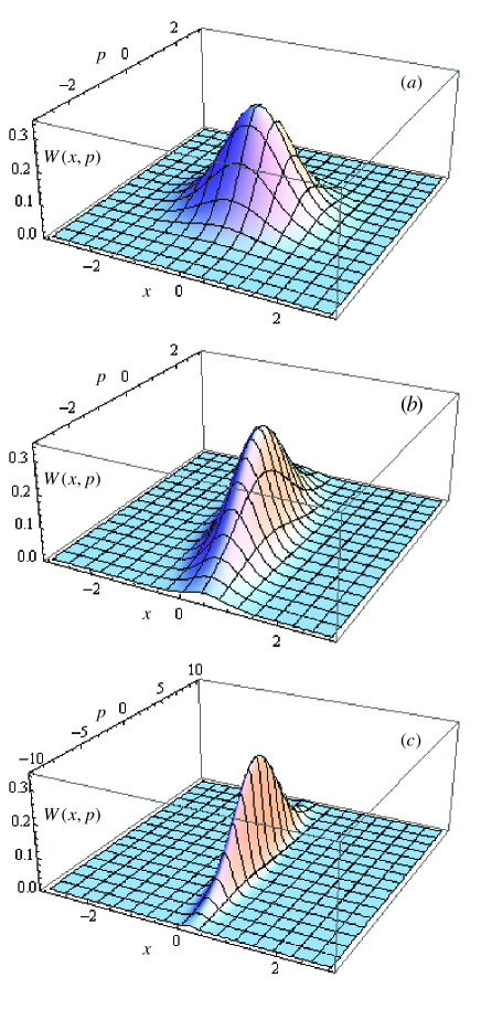
Figure 1: (Color online) Wigner function of the squeezed state for the CK Hamiltonian model for $n=0$ (a) $\gamma=0,$ $t=0;$ (b) $\gamma=0.5,$ $t=1;$(c)$\gamma=0.5,$ $t=3.$

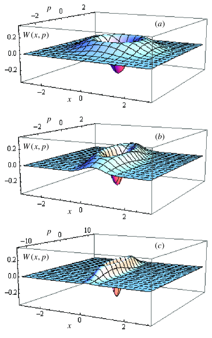
Figure 2: (Color online) Wigner function of the squeezed state for the CK Hamiltonian model for $n=1$ (a) $\gamma=0,$ $t=0;$(b)$\gamma=0.5,$ $t=1;$(c)$\gamma=0.5,$ $t=3.$

V Conclusion

In summary, we have introduced the time-dependent Fresnel operator for converting Caldirola-Kanai Hamiltonian into time-independent harmonic oscillator Hamiltonian, the $A,B,C,D$ parameters involved in the Fresnel operator are the solution to a set of the patrial differential equations set up in the above mentioned converting process. In this way the dynamics of Caldirola-Kanai Hamiltonian is solved, Our method may be suitable for solving the Schrödinger equation of other time-dependent oscillators.

Acknowledgments This work was supported by the the National Natural Science Foundation of China under Grant Nos.10775097, 10874174 and Shandong Provincial Natural Science Foundation, China Grant No.ZR2010AQ024.

References

• (1) P. Caldirol, Nuovo Cimento 18, 394 (1941).
• (2) E. Kanai, Prog. Theor. Phys. 3, 440 (1948).
• (3) H. R. Lewis, and W. B. Riesenfeld, J. Math. Phys. 10, 1458 (1969).
• (4) K. H. Yeon, C. I. Um, and T. F. George, Phys. Rev. A 36, 5287 (1987).
• (5) C. C. Gerry, P. K. Ma, and E. R. Vrscay, Phys. Rev. A 39, 668 (1989).
• (6) I. A. Pedrosa, G. P. Serra, and I. Guedes, Phys. Rev. A 56, 4300 (1997).
• (7) K. H. Yeon, D. F. Walls, C. I. Um, T. F. George, and L. N. Pandey, Phys. Rev. A 58, 1765 (1998).
• (8) C. I. Um, K. H. Yeon and T. F. George, Phys. Rep. 362, 63 (2002) and references therein.
• (9) S. P. Kim, J. Phys. A Math. Gen. 36, 12089 (2003).
• (10) J. R. Choi, and K. H. Yeon, Phys. Rev. A 79, 054103 (2009).
• (11) H. Y. Fan, H. L. LU, and Y. Fan, Ann. Phys. 321, 480 (2006).
• (12) H. Y. Fan, Ann. Phys. 323, 500 (2008).
• (13) J. R. Klauder and Bo-Sture Shagerstam, Coherent States (World Scientific, Singapore, 1985)
• (14) H. Y. Fan, and J. V .Linde, Phys. Rev. A 39, 2987 (1989).
• (15) H. Y. Fan, and H. L. Lu, Opt. Commu. 258, 51 (2006).
• (16) H. Y. Fan, H. L. LU, and Y. Fan, Ann. Phys. 321, 480 (2006).
• (17) D. F. V. James and G. S. Agarwar, Opt.Commun. 126, 207 (1996)
• (18) H. Y. Fan, H. L. LU, Int. J. Theor. Phys. 45, 641 (2006).
• (19) E. Wigner, Phys. Rev 40, 749 (1932).