Ionisation feedback in star formation simulations: The role of diffuse fields

Abstract

We compare the three-dimensional gas temperature distributions obtained by a dedicated radiative transfer and photoionisation code, MOCASSIN, against those obtained by the recently-developed Smooth Particle Hydrodynamics (SPH) plus ionisation code iVINE for snapshots of an hydrodynamical simulation of a turbulent interstellar medium (ISM) irradiated by a nearby O star.

Our tests demonstrate that the global ionisation properties of the region are correctly reproduced by iVINE, hence validating further application of this code to the study of feedback in star forming regions. However we highlight potentially important discrepancies in the detailed temperature distribution. In particular we show that in the case of highly inhomogenous density distributions the commonly employed on-the-spot (OTS) approximation yields unrealistically sharp shadow regions which can affect the dynamical evolution of the system.

We implement a simple strategy to include the effects of the diffuse field in future calculations, which makes use of physically motivated temperature calibrations of the diffuse-field dominated regions and can be readily applied to similar codes. We find that while the global qualitative behaviour of the system is captured by simulations with the OTS approximation, the inclusion of the diffuse field in iVINE (called DiVINE) results in a stronger confinement of the cold gas, leading to denser and less coherent structures. This in turn leads to earlier triggering of star formation. We confirm that turbulence is being driven in simulations that include the diffuse field, but the efficiency is slightly lower than in simulations that use the OTS approximation.

1 Introduction

Ionising radiation from OB stars influences the surrounding interstellar medium (ISM) on parsec scales. As the gas surrounding a high mass star is heated, it expands forming an HII region. The consequence of this expansion is twofold, on the one hand gas is removed from the centre of the potential preventing it from further gravitational collapse. On the other hand gas is swept up and compressed beyond the ionisation front producing high density regions that may thus be susceptible to gravitational collapse (i.e. the “collect and collapse” model, Elmegreen et al 1995). Furthermore, pre-existing, marginally gravitationally stable, clouds may also be driven to collapse by the advancing ionisation front (i.e. “radiation-driven implosion”, Bertoldi 1989, Kessel-Deynet & Burkert 2003, Gritschneder et al 2009a). Finally, ionisation feedback is also thought to be a driver for small scale turbulence in a cloud (Gritschneder et al 2009b). The net effect of photoionisation feedback on the global star formation efficiency is still, however, under debate.

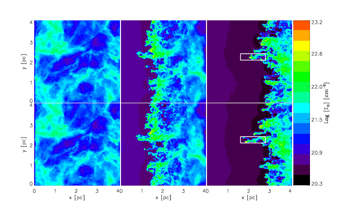
Figure 1: Surface density projected in the z-direction of the t =9 kyr (left), 250 kyr (middle) and  500 kyr (right) snapshots of G09b’s turbulent ISM simulation. The upper panels show the evolution of the gas without diffuse field, the lower panels show the same simulation performed with the simplified diffuse field implementation discussed in Section 4. The white boundaries on the left-hand panels mark the regions compared in Table 1. The SPH particles were mapped onto a 128³ regular Cartesian grid.

While the importance of studying the photoionisation process as part of hydrodynamical star formation simulations has long been widely recognised, until very recently, due to the complexity and computational demand of the problem, the evolution of ionised gas regions had only been studied in rather idealised systems (e.g. Yorke et al. 1989; Garcia-Segura & Franco 1996), with simulations often lacking resolution and dimensions. Fortunately, the situation in the latest years has been rapidly improving, with more sophisticated implementations of ionised radiation in grid-based codes presented by (e.g.) Mellema et al (2006), Krumholz et al (2007) and Peters et al (2010).

Kessel-Deynet & Burkert (2000) were the first to introduce an ionisation algorithm into a Smoothed Particle Hydrodynamical (SPH) code to study radiation-driven implosion as a possible trigger of star formation. Later, Dale, Ercolano & Clarke (2007) presented a much simplified, but fast, algorithm to consider photoionisation within complex SPH simulations. When compared to grid codes, which are based on the solution of the Eulerian form of the same equations, much higher resolution of very complex flows can be achieved. Since Dale et al (2007) a number of other ionising radiation implementations have been developed for SPH codes, including Pawlik & Schaye (2008), Altay et al. (2008), Bisbas et al (2009) and very recently Gritschneder et al (2009a). However high resolution SPH simulations are very computationally expensive, and even in the current era of parallel computing, an exact solution of the radiative transfer (RT) and photoionisation (PI) problem in three dimensions within SPH calculations is still prohibitive. Necessarily, all the algorithms mentioned above employ an extremely simplified approach to RT and PI. The consequences of such simplification on the conclusions drawn from the simulations need to be investigated.

In Dale et al (2007), we performed the only such verification to date against a fully three-dimensional radiative transfer and photoionisation code (MOCASSIN, Ercolano et al 2003, 2005 and 2008) for complex density fields obtained from the SPH calculations. We showed in that case that the agreement on the ionised fractions in high density regions was very good, but low density regions were poorly represented by the ionisation + SPH code. In this paper we take a similar approach to test the more recent algorithms developed in iVINE (Gritschneder et al. 2009a). We find excellent agreement between the codes for the global ionisation fractions, however we highlight discrepancies in the temperature distribution, particularly in shadow regions that are dominated by the diffuse field, which is not accounted for in iVINE. We test the consequences of the omission of the diffuse field both on the hydrodynamical evolution of the structure and on the evolution of the turbulence spectrum using a simple approach that allows for a more realistic, but still efficient modelling strategy of the shadow regions.

In Section 2 we briefly describe the iVINE and MOCASSIN codes and the comparison strategy. In Section 3 we show the results of this comparison. In Section 4 we discuss a simple approach to qualitatively include diffuse field effects in iVINE and show the results from these further tests in Section 5. Section 6 contains a brief summary and future directions.

2 Numerical Methods

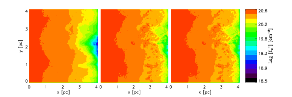
Figure 2: Surface density of electrons projected in the z-direction for the G09b turbulent ISM simulation at t = 500 kyr (bottom panels of Figure 1). Left: iVINE; Middle: MOCASSIN H-only; Right: MOCASSIN nebular abundances.

We have used the MOCASSIN code (Ercolano et al 2003, 2005, 2008a) to calculate the temperature and ionisation structure of the turbulent ISM density fields presented by Gritschneder et al (2009b, from now on G09b) and Gritschneder et al (2010). The SPH quantities were obtained with the iVINE code (Gritschneder et al 2009a) and mapped onto a regular 128³ Cartesian grid. We briefly describe the set-up of the two codes and summarise the strategy for our comparative tests.

2.1 iVINE

iVINE (Gritschneder et al 2009a) is a highly efficient fully parallel implementation of ionising radiation in the tree-SPH code VINE (Wetzstein et al 2009, Nelson et al 2009). While the treatment of hydrodynamics and gravitational forces is fully three-dimensional the UV-radiation of a massive star is assumed to impinge along parallel rays onto the simulated domain. To keep the computational effort small the radiation is assumed to be monochromatic. In addition, ionising photons reemitted following recombinations are assumed to be immediately absorbed in the direct neighbourhood (on-the-spot approximation, e.g. Spitzer 1978). On the surface of infall the domain is decomposed into small rays. Along these rays the radiation is propagated from SPH-particle to SPH-particle by iterating the ionisation degree to its equilibrium value. This is done at the smallest hydrodynamical time-scale, i.e. after each hydrodynamical time-step. The newly found ionisation degree $\eta$ is then coupled to the hydrodynamic evolution via the gas pressure of each individual particle i:

$$P_{\mathrm{i}}=\left(\frac{T_{\mathrm{hot}}\eta_{\mathrm{i}}}{\mu_{\mathrm{hot}}}+\frac{T_{\mathrm{cold}}(1-\eta_{\mathrm{i}})}{\mu_{\mathrm{cold}}}\right)\frac{k_{\mathrm{B}}\rho_{\mathrm{i}}}{m_{\mathrm{p}}},$$ (1)

where $T_{hot}$ = 10kK and $T_{cold}$ = 10K and $\mu_{\mathrm{hot}}=0.5$ and $\mu_{\mathrm{cold}}=1.0$ are the temperatures and the mean molecular weights of the ionised and the un-ionised gas in the case of pure hydrogen, respectively. $k_{\mathrm{B}}$ is the Boltzmann constant, $m_{\mathrm{p}}$ is the proton mass and $\rho_{\mathrm{i}}$ is the SPH-density of the particle. To ensure a correct treatment of the newly ionised particles, their time-step is reduced according to the ratio of the sound-speeds in the hot and the cold gas. For a detailed description along with numerical tests see Gritschneder et al (2009a). The accuracy parameters for the simulations presented here are as given in G09b.

To map the complex particles distribution obtained with the iVINE code on a equally spaced Cartesian grid we bin the particles weighted with the SPH kernel. For each particle the grid cells which are inside the particles smoothing length are determined. Onto these cells the mass of the SPH particle is then distributed according to a weight obtained by equating the kernel for the given distance between particle and grid cell. All other quantities are weighted accordingly.

2.2 MOCASSIN

MOCASSIN is a three-dimensional photoionisation and dust radiative transfer code that employs a Monte Carlo approach to the frequency resolved transfer of radiation. The code includes all the dominant microphysical processes that influence the gas ionisation balance and the thermal balance of dust and gas, including processes that couple the gas and dust phases. In the case of HII regions ionised by OB stars the dominant heating process for typical gas abundances is photoionisation of hydrogen, which is balanced by cooling by collisionally excited line emission (dominant), recombination line emission, free-bound and free-free emission. The atomic database includes opacity data from Verner et al. (1993) and Verner & Yakovlev (1995), energy levels, collision strengths and transition probabilities from Version 5.2 of the CHIANTI database (Landi et al. 2006, and references therein) and the improved hydrogen and helium free-bound continuous emission data of Ercolano & Storey (2006). The code was originally developed for the detailed spectroscopic modelling of ionised gaseous nebulae (e.g. Ercolano et al 2004, 2007), but is regularly applied to a wide range of astrophysical environments, including protoplanetary discs (e.g. Ercolano et al 2008b, 2009, Owen et al 2010, Schisano et al 2010) and supernova envelopes (e.g. Sugerman et al 2006, Ercolano et al 2007b, Wesson et al 2009, Andrews et al 2010). Arbitrary ionising spectra can be used as well as multiple ionisation sources whose ionised volumes may or may not overlap, with the overlap region being self-consistently treated by the code. Arbitrary dust abundances, compositions and size distributions can be used, with independent grain temperatures calculated for individual grain sizes.

In order to compare with iVINE, the stellar field was assumed to be incident along parallel rays, but the subsequent RT was performed in three dimensions hence allowing for an adequate representation of the diffuse field. We scaled the incoming stellar field to the value used by G09b ($F_{Ly}$ = 5$\times$10⁹ phot/cm²/sec) and we assumed a blackbody spectrum of 40kK. The exact choice of the blackbody temperature (within the range of typical effective temperatures for OB stars) does not have a significant impact for our application. We did not include dust grains in the calculation in order to allow a more immediate comparison with iVINE.

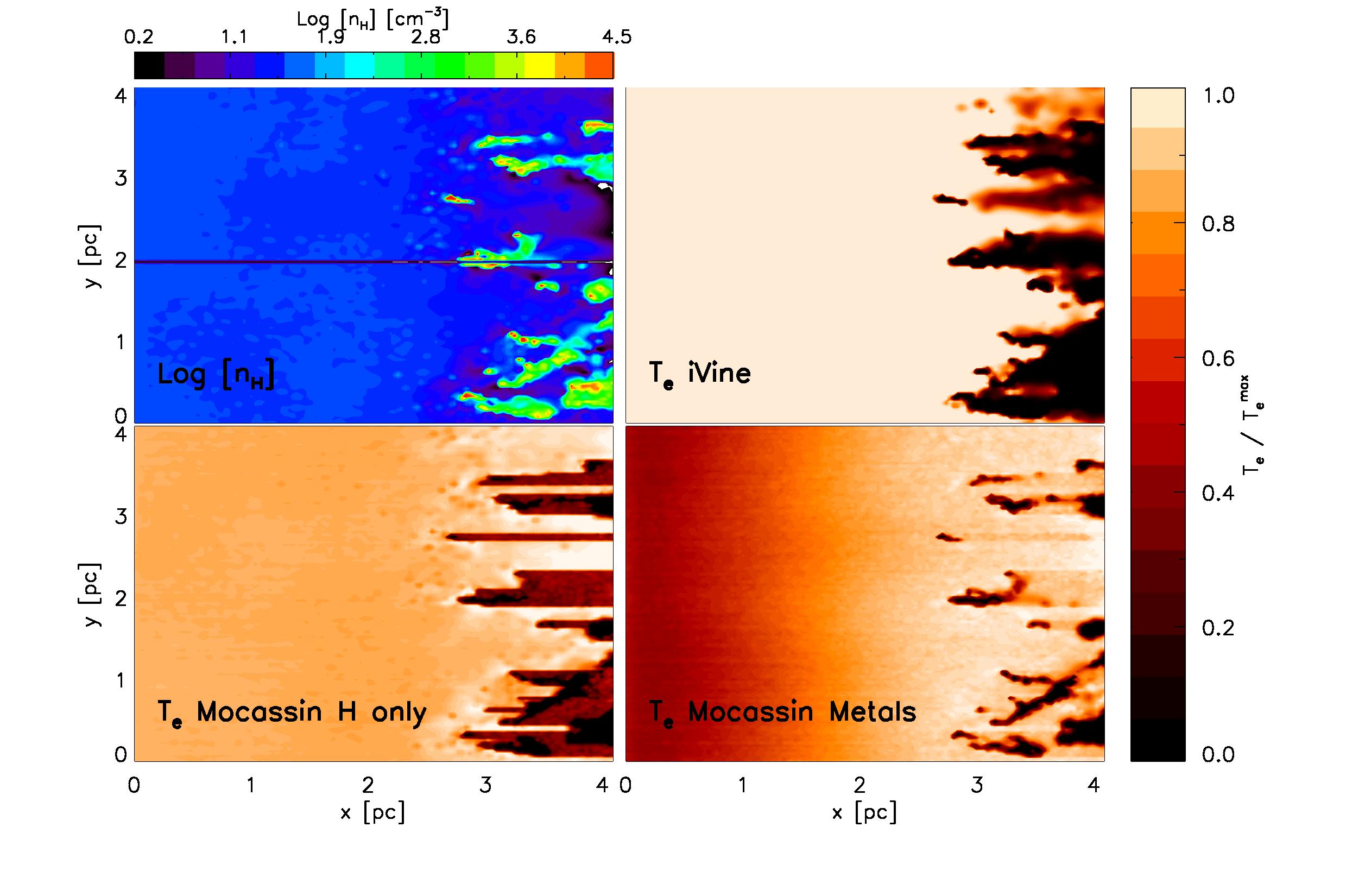
Figure 3: Density and temperature maps for the z = 25 slice of the G09b turbulent ISM simulation at t = 500 kyr. Top left: Gas density map; Top right: electron temperature, $T_{e}$ as calculated by iVINE;; Bottom left: electron temperature, $T_{e}$ as calculated by MOCASSIN with H-only; Bottom right: electron temperature, $T_{e}$ as calculated by MOCASSIN with nebular abundances. The solid black horizontal line shows the location chosen for the plots shown in Figure 4.

2.3 Strategy for comparison test

The comparisons are based on the simulations of G09b which address the impact of ionising radiation on a turbulent ISM. These simulations used $2\times 10^{6}$ SPH-particles, which are set up to resemble a medium with an average number density of $300cm^{-3}$ in a volume of $(4pc)^{3}$. To mimic turbulence, a supersonic velocity field with Mach 10 is set up on the largest modes. This setup is allowed to decay freely down to a turbulent Mach number of 5 before the ionisation field is switched on. We have taken snapshots of this simulation at several time-steps and mapped the corresponding SPH particle fields to a 128³ Cartesian grid.

We have taken snapshots at several time-steps in the turbulent ISM simulation of G09b and mapped the corresponding SPH particle fields to a 128³ Cartesian grid. Figure 1 shows the surface density projected in the z-direction for the t = 9 kyr (left), t = 250 kyr (middle), and t = 500 kyr (right) snapshots. The top panels show the results from the original G09b calculation (no diffuse field), while the bottom panels show the same results for the approximate diffuse field calculation presented in Section 4. The comparison tests discussed in Section 3 were performed using the distributions from the original G09b calculation shown in the top panels.

Three-dimensional RT and PI calculations were performed on the Cartesian grid using MOCASSIN as described above. We run H-only simulations (referred to as “H-only”) as well as simulations with typical HII region abundances (referred to as “Metals”). The elemental abundances for the metal-rich model were as follows, given as number density with respect to Hydrogen: He/H = 0.1, C/H = 2.2e-4, N/H = 4.0e-5, O/H = 3.3e-4, Ne/H = 5.0e-5, S/H = 9.0e-6.

We compared the resulting MOCASSIN temperature and ionisation structure grids to iVINE with the aim to address the following questions: (i) Are the global ionisation fractions accurate? (ii) How accurate is the gas temperature distribution? (iii) What is the effect of the diffuse field? (iv) How can the algorithm be improved?

3 Results

In this section we present the results of our comparison of the original G09b iVINE calculations (top panels in Figure 1) with MOCASSIN. We limit the discussion to the t = 500 kyr snapshot, but we note here that the same conclusions apply to the other timesteps (we have performed the same tests at several time snapshots).

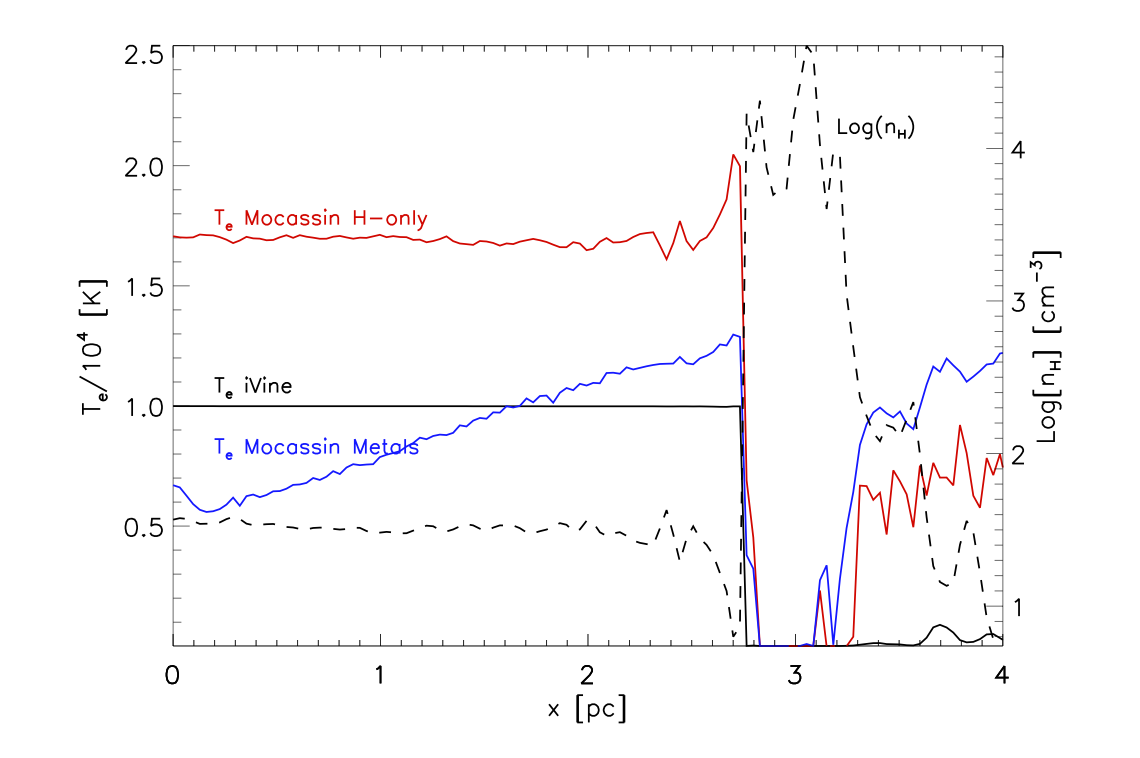
Figure 4: Density and temperature profile along a typical ray of the G09b turbulent ISM simulation at t = 500 kyr. The black dashed line shows the density profile, the black solid line shows the temperature profile calculated by iVINE the solid red and blue profile show the temperature profiles calculated by MOCASSIN with H-only and nebular abundances, respectively.

3.1 Global Properties

Figure 2 shows the surface density of electrons projected in the z-direction for the G09b turbulent ISM simulation at t = 500 kyr. The figure shows that the integrated ionisation structure is reasonably well reproduced by iVINE. There are however some qualitative differences at the rear of the grid (X¿3 pc) where iVINE predicts a lower surface density of electrons (i.e. a more neutral gas). This is due to the fact that these regions are completely shielded from ionising photons in VINE by overlapping shadows. In the mocassin simulations, however, reprocessed photons are able to diffuse amongst the clumps and reach the rear of the domain. Nevertheless, these differences are small and the global ionisation structure is correctly determined by iVINE, as confirmed by the simple comparison of the total ionised mass fractions: at t = 500 kyr, iVINE obtains a total ionised mass of 13.9%, while MOCASSIN “H-only” and “Metals” obtain 15.6% and 14.0%, respectively. The agreement at other time snapshots is equally good (e.g. at t = 250 kyr iVINE obtains 9.1% and MOCASSIN “Metals” 9.5%).

It may at first appear curious that the agreement should be better between iVINE and MOCASSIN “Metals”, rather than MOCASSIN “H-only”, given that only H-ionisation is considered in iVINE. This is however simply explained by the fact that iVINE adopts an “ionised gas temperature” ($T_{hot}$) of 10kK, which is close to a typical HII region temperature, with typical gas abundances. The absence of metals in the MOCASSIN “H-only” simulations causes the temperature to rise to typical values close to 17kK, due to the fact that cooling becomes much less efficient without collisionally excited lines of oxygen, carbon etc. The hotter temperatures in the “H-only” models directly translate into slower recombinations, as the recombination coefficient is roughly proportional to the inverse of the temperature. As a result of slower recombinations the “H-only” grids have a slightly larger ionisation degree.

3.2 Ionisation and temperature structure

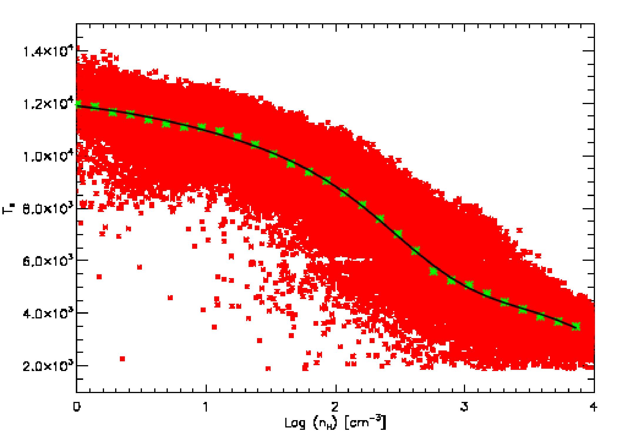
Figure 5: Temperature versus density distribution of the shadowed cells. The red points are the values for each cell as calculated by MOCASSIN with nebular abundances; the green points represent the binned data and the black solid line represents a Gaussian fit to the binned data.

The gas temperature of a particle in iVINE is calculated as a simple function of the ionisation fraction, $\eta$ i.e.

$$T_{e}=T_{hot}\cdot\eta+T_{cold}\cdot(1-\eta)$$ (2)

where $T_{hot}$ = 10kK and $T_{cold}$ = 10K are the temperatures assigned to fully ionised and neutral material, respectively. Accurate gas temperatures are of prime importance as this is how feedback from ionising radiation impacts on the hydrodynamics of the system (cf Eq. 1). In Figure 3 we compare the electron temperatures $T_{e}$ calculated by iVINE and MOCASSIN (“H-only” and “Metals”) in a z-slice of the t = 500kyr grid. The top-right panel of the figure shows the volumetric number density [cm^-3] map for the selected slice. The large shadow regions behind the high density clumps in the iVINE calculations are immediately evident in the figure. These shadows are largely reduced in the MOCASSIN calculations as a result of diffuse field ionisation. The diffuse field is softer than the stellar field and therefore temperatures in the shadow regions are lower than in the directly illuminated regions. Figure 4 shows a more quantitative comparison of the temperature distribution along a single ray intercepting a high density clump and its shadow region. The ray is marked in Figure 3 as the solid black line in the top left panel. The dashed line in Figure 4 shows the logarithmic hydrogen number density as a function of distance into the grid. The solid black solid line is the electron temperature along the ray as determined by iVINE, while the solid red and blue lines are the electron temperatures determined by MOCASSIN “H-only” and “Metals”, respectively. The higher temperatures in the shadow regions of the MOCASSIN “Metals” model are a consequence of the Helium Lyman radiation and the heavy elements free-bound contribution to the diffuse field.

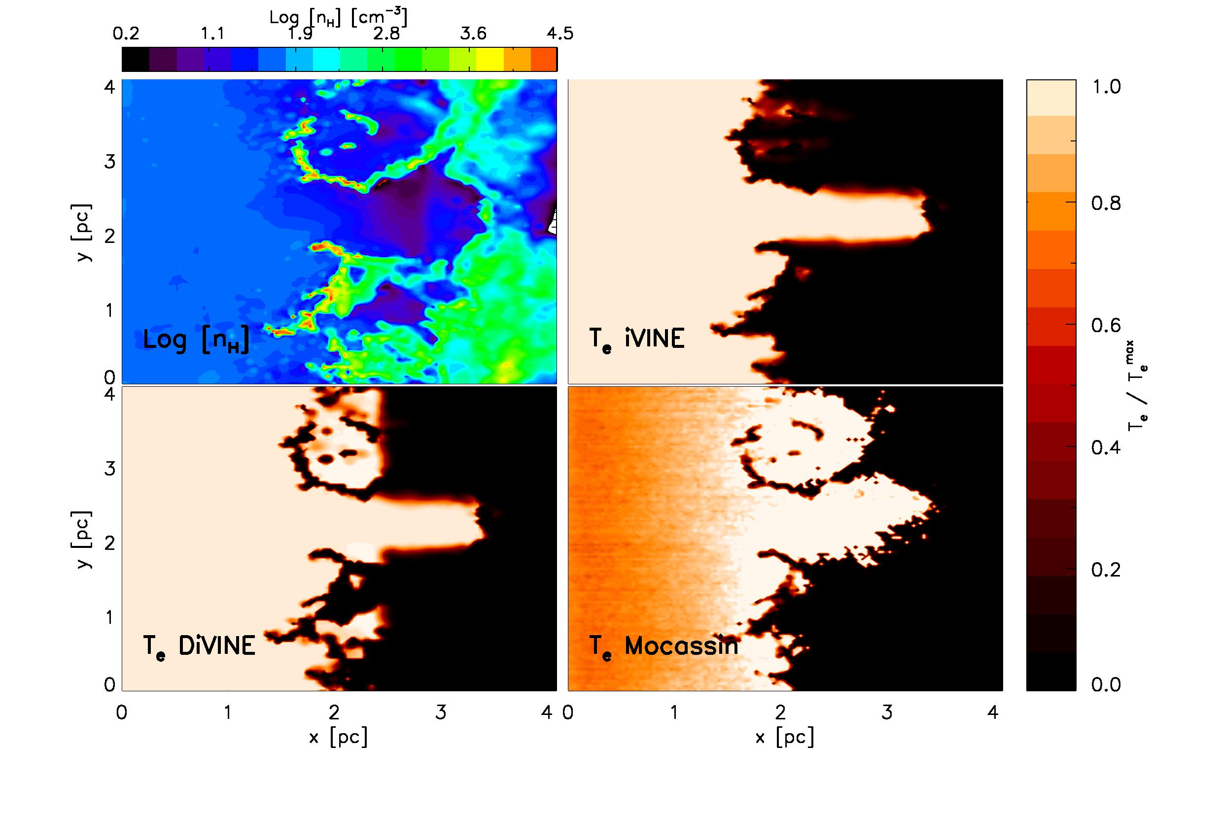
Figure 6: Density and temperature maps for the z = 25 slice of the G09b turbulent ISM simulation at t = 250 kyr. Top left: Gas density map; Top right: electron temperature, $T_{e}$ as calculated by iVINE;; Bottom left: electron temperature, $T_{e}$ as calculated by DiVINE; Bottom right: electron temperature, $T_{e}$ as calculated by MOCASSIN with nebular abundances.

The effects of radiation-hardening and of the recombination of some of the important cooling ions is also apparent in MOCASSIN’s temperatures which rise with distance from the star in the directly illuminated regions. As expected the effect is much more pronounced in the “Metals” model (a steeper temperature distribution in metal-rich regions is a well known effect, e.g. Stasinska 2005, Ercolano et al 2007). Radiation hardening is accounted for in some “monochromatic” RT codes, by pre-calculating the effective photoionisation x-section as a function of the Lyman-limit optical depth by integrating over the extinguished stellar spectrum, and doing the same for the photoelectric heating integral (e.g. C2Ray, Mellema et al. 2006). Helium, heavy elements or dust effects are not included, by this treatment however and most importantly the effects of different coolants acting in different regions (which is dominating the temperature distribution in the directly illuminated regions of the MOCASSIN Metals calculations) cannot be accounted for in this way. In future work we plan to provide simple temperature calibrations to account for the environmentally driven temperature gradients in the directly illuminated regions. We note however that errors in the temperature of the directly illuminated regions are unlikely to exceed factors of two at most, the errors on the temperature of the diffuse field dominated regions, on the other hand, are typically three orders of magnitude (10K compared to 10kK). Thus, in the remainder of this paper we shall focus on the larger temperature differences in the shadowed regions and how they may affect the hydrodynamical evolution of the system.

4 Gas temperatures in shadow regions

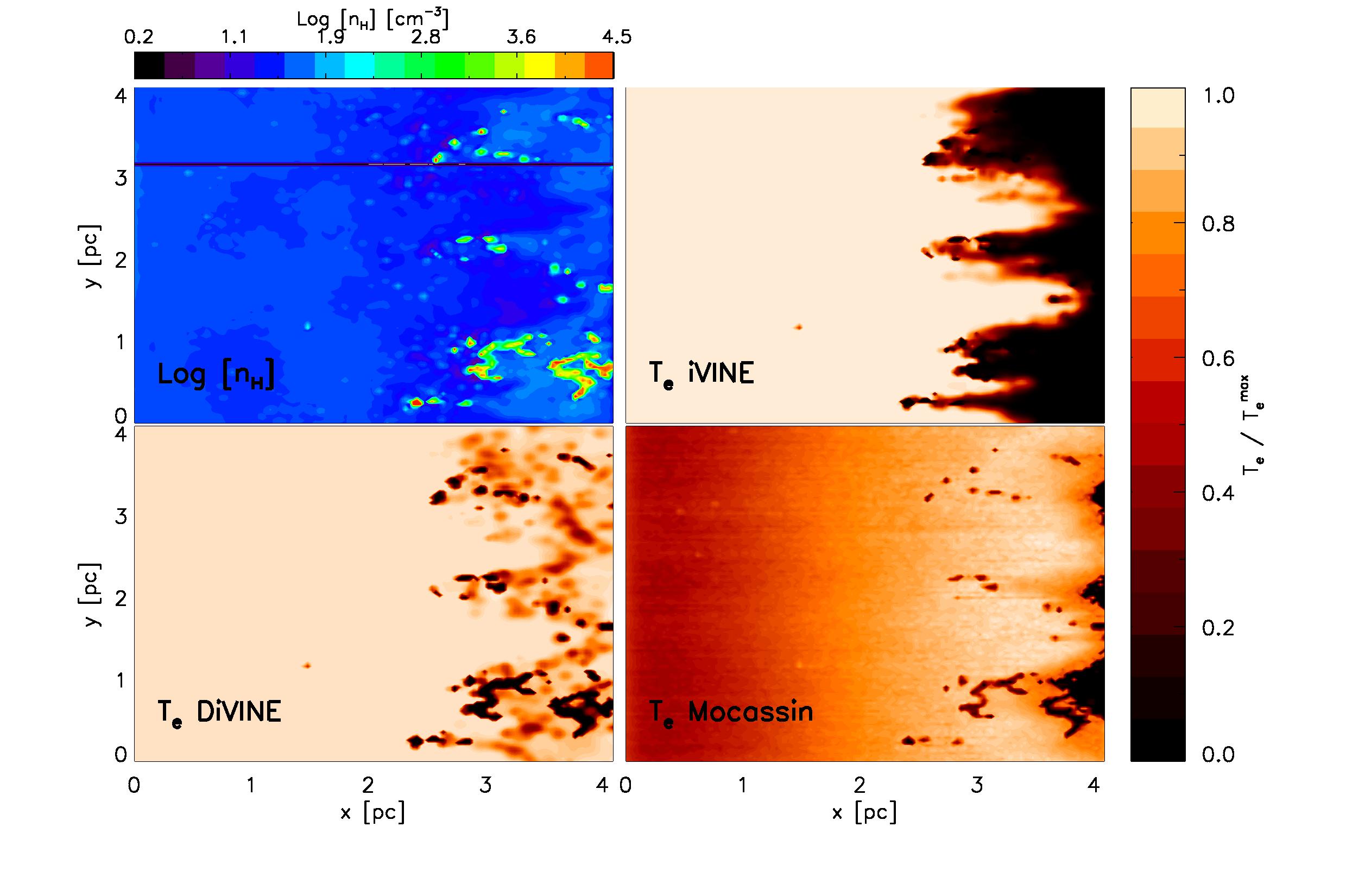
Figure 7: Density and temperature maps for the z = 25 slice of the G09b turbulent ISM simulation at t = 500 kyr. Top left: Gas density map; Top right: electron temperature, $T_{e}$ as calculated by iVINE;; Bottom left: electron temperature, $T_{e}$ as calculated by DiVINE; Bottom right: electron temperature, $T_{e}$ as calculated by MOCASSIN with nebular abundances.

As iVINE solves the transfer along plane parallel rays using the on-the-spot approximation (e.g. Spitzer 1978, Osterbrock & Ferland 2006, page 26), it has currently no means of bringing ionisation (and hence heating) to regions that lie behind high density clumps. This creates sharp shadows with a large temperature (pressure) gradient between neighbouring direct and diffuse-field dominated regions, which may have important implications for the dynamics, particularly with respect to turbulence calculations.

In order to explore the significance of the error introduced by the OTS approximation on the dynamics of the system, we propose here a simple strategy to include the effects of the diffuse field in iVINE, which can be readily extended to other similar codes. It can be summarised in the following steps: (i) identify the diffuse field dominated regions (shadow); (ii) study the realistic temperature distribution in the shadow region using fully frequency resolved three-dimensional photoionisation calculations performed with MOCASSIN and parameterise the gas temperature in the shadow regions as a function of (e.g.) gas density; (iii) implement the temperature parameterisation in iVINE and update the gas temperatures in the shadow regions at every dynamical time step accordingly.

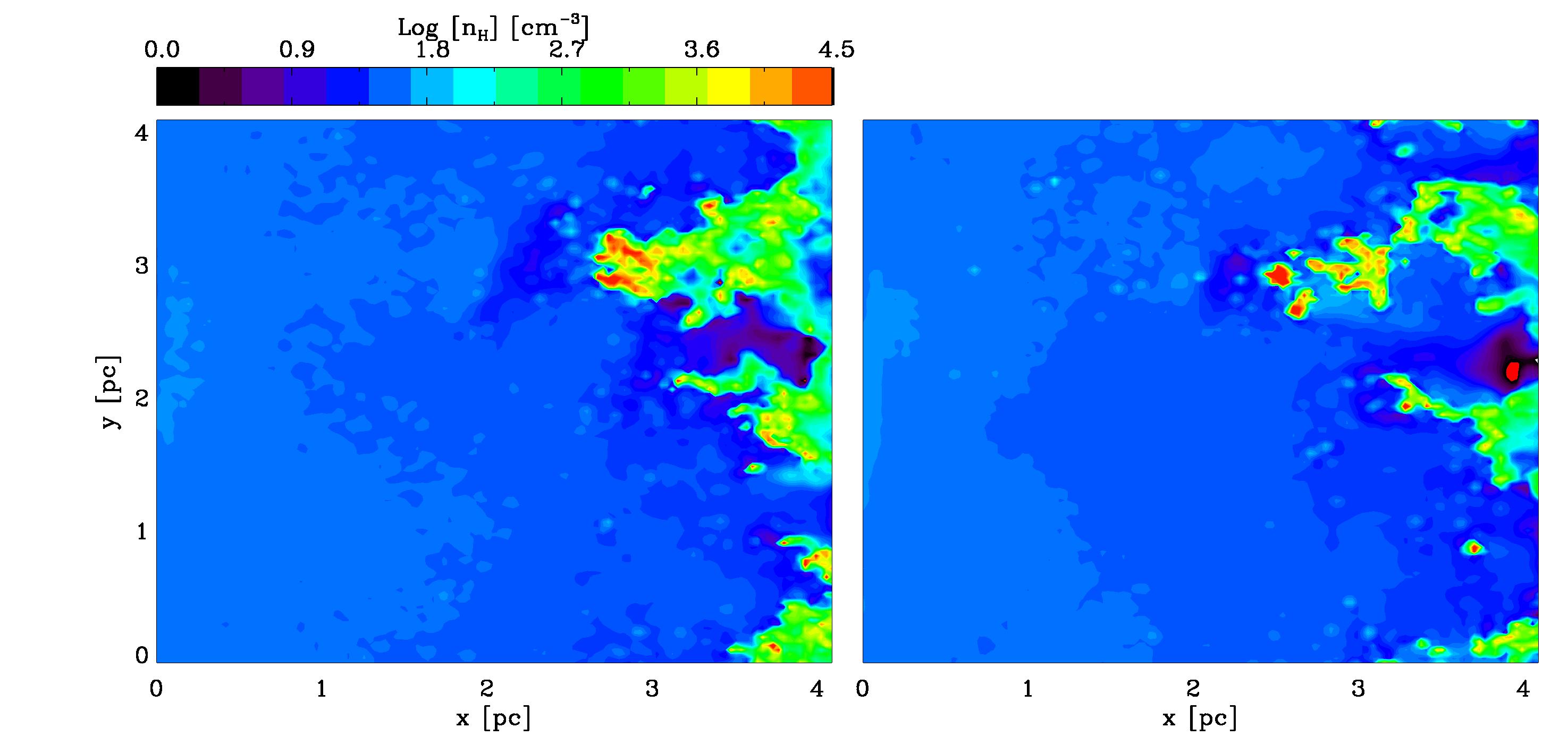
Figure 8: Volume density slices at t = 500kyr for the iVINE (left) and DiVINE (right) runs.

In what follows we describe our zeroth order implementation of the above strategy for the case at hand, but we stress that this can be adapted to different situations. In future work we will present a generalised version of the procedure detailed below, which will include temperature parameterisations for both the direct and diffuse-field dominated regions and will account for different environments and geometrical setups of the codes. This requires a parameter space study and is beyond the scope of the current work, where we only aim to assess the relevance of relaxing the OTS approximation for highly inhomogenous cases.

4.1 Step i: Identify the shadows

In the case of iVINE, we identify the diffuse-field dominated regions by means of simple criteria that need only be evaluated along a ray, such that no significant overheads are introduced by this step. A particle / grid-cell is initially defined to be ’shadowed’ if iVINE would assign a temperature of $T<100$ K to it, i.e. if its ionisation degree is $\eta<10^{-2}$.

4.2 Step ii: Study the temperature structure in the shadows

We study the MOCASSIN-determined temperature structure of the shadow regions identified in Step i, for several time snapshots in the G09b simulation. For each snapshot we plot the gas temperature against density for all the shadowed cells in the entire grid. Figure 5 shows the results for the t = 500 kyr snapshot. The red marks represent each individual grid cell in the MOCASSIN grid, while the yellow asterisks represent the averaged value, which is then fit by the curve shown by the solid line. The fit was obtained by a six term Gaussian fit of the form:

$$y=A_{0}*exp(-(z^{2})/2)+A_{3}+A_{4}x+A_{5}x^{2}$$ (3)

where x = $T_{e}$, y = $Log(n_{H})$, z = (x - A₁)/A₂ . The fit coefficients for the curve shown are A₀= -4378.10, A₁= -0.0275, A₂= 0.616, A₃= 17715.8, A₄ = -5322.37, A₅ = 395.13. The form of this relationship does not vary much for different time snapshots and it is mainly controlled by the shape of the direct field and the metallicity of the region.

The near-invariance of the T_e-n_H relation at different times is certainly encouraging, however a number of caveats need also be noted here. Most importantly the fact that not all of the shadow cells identified in Step i obey Eqn 3. A large fraction of these cells are in fact truly shadowed and have temperatures of $<$100 K also according to MOCASSIN (these cells lie below the lower y-axis cutoff in Figure 5). These are cells that are located in regions where the diffuse photons cannot penetrate, thus, in this respect, applying our simple shadow region criteria indiscriminately to all gas would severely overestimate the thermal effects of the diffuse field. We thus apply a further density criterion that only allows low density cells ($n_{H}<100cm^{-3}$) to be heated by the diffuse field. This is justified by the fact that our grids show that the number of cells that follow Equation 3 varies according to the density of the cell. At t = 500 kyr we find that over 90% of cells with n${}_{H}<10cm^{-3}$, obey Equation 2, this goes down to 75% for cells with $10cm^{-3}<$ n${}_{H}<100cm^{-3}$ and then down to less than 10% for cells with n${}_{H}>100cm^{-3}$. While this density cut-off will still slightly overestimate the effect of the diffuse field in the $10cm^{-3}<$ n${}_{H}<100cm^{-3}$ regime, we note that a temperature of 10 K is only really expected for dark cloud conditions, perhaps met only in the higher densities regions in the simulations. The rest of the gas at lower densities in the true shadow zone (i.e. those cells that do not obey Equation 2) is more realistically described by photon dominated region (PDR) conditions, with temperatures closer to 1000 K, rather than 10 K. So the error introduced by applying Equation 2 to the true shadow zone in the $10cm^{-3}<$ n${}_{H}<100cm^{-3}$ range is still smaller than if those cells had been assigned their original temperature of 10 K.

A second order problem is posed by the large scatter of the data (red points) shown in Figure 5. Typical errors of $\sim$50% in temperature are to be expected with this method.The temperature at a given location in an ionised region is expected to roughly scale with the local ionisation parameter, which is defined as the ratio of the ionising flux to the gas density at that location. A temperature-density relation as the one shown in Figure 5 thus ignores the local variations of the diffuse field intensity and shape. The large scatter shown in Figure 5 is therefore a shortcoming of this method, but has the advantage of avoiding the large computational overheads of a full diffuse field calculation. We stress, however, that the effect of these errors on the dynamics is not large. Again, the error introduced by assuming the particle to be in the cold phase due to the lack of diffuse radiation is much larger than the spread in this relation.

4.3 Step iii: Implement temperature corrections

Once a simple description of the temperature distribution in the shadow region is available from Step ii, this can be implemented as a correction to the SPH temperatures and thus pressure. In the case of the current iVINE implementation this simply requires that at every dynamical time step, all particles that fulfil the criteria defined in Steps i and ii be identified and their temperature re-assigned according to the parameterised curve obtained in Step ii. To avoid unphysical heating far beyond the ionisation front, we impose an additional constraint. A particle only gets heated if the total ionised mass inside the current slab perpendicular to the in-falling radiation is smaller then the diffusively heated mass inside this slab. Note that this constraint implies that in the last diffusively heated slab all radiation emitted by recombinations is only absorbed in the adjacent cold structures and not in the hot surrounding gas. This therefore represents the case for maximum efficiency for the diffuse radiation, but, as demonstrated in Section 5.1, we find that no significant overheating of the shadows is introduced by our procedure.

We note that this approach in principle allows for environmental variables, such as the hardness of the stellar field and the metallicity and dust content of the gas to be accounted for in the SPH calculation, since their effect on the temperature distribution is folded in the parameterisation obtained with MOCASSIN. In most cases however, environmental effects on the temperature may be smaller than the scatter showed by the temperature points in Figure 5.

In the simple implementation of the method presented here, we apply a density cut to the particles to be heated by the diffuse field, which allows us to use a rough but fast criterion for the identification of the diffuse field dominated particles without over-estimating the effects of the diffuse field. As shown in Figure 5, the temperature only varies by approximately 50% for number densities lower than 100 cm^-3, meaning that the qualitative behaviour of the system would not change significantly if an average value for the temperature were to be used in place of Equation 3. The application of Equation 3, however, does not add a significant computational overhead and it is therefore preferred here in view of future calculations where we aim at refining the method to allow the application of a temperature correction to the whole density range, where the temperature variation is larger and the application of a single temperature value would yield larger errors.

5 Diffuse field effects on hydrodynamics

We have compared the results of the original iVINE run with those obtained after implementing the diffuse field strategy outlined in the previous section. We will refer to the diffuse field implementation of iVINE as DiVINE (Diffuse field iVINE).

5.1 Temperature structure in the shadows

As an a-posteriori check of the diffuse field implementation in DiVINE, we compare the gas temperatures at individual slices in the simulation at times 250 and 500 kyr in Figures 6 and 7, respectively. The top right and bottom left and right panels show the gas temperatures calculated using iVINE, DiVINE and MOCASSIN, respectively, for the density field shown in the top left panels. We find that, while there are still some obvious differences between the DiVINE and MOCASSIN results, the improvement over the original iVINE runs is certainly encouraging, particularly when considering the minimal computational overhead introduced by this procedure. We also note that the diffuse field heated mass in DiVINE and MOCASSIN are very similar.

Some noticeable differences can be seen in Figures 6 and 7 include a hot region predicted by DiVINE in Figure 6 approximately at (x,y) = (2.2, 0.7) pc which is not present in ’mocassin and cooler regions at large x predicted by  mocassin in Figure 7. These are both examples in which material in the true shadow has been erroneously been heated by our diffuse field algorithm in DiVINE. This only represents a small quantity of gas and has no significant effect on the dynamical evolution of the system.

5.2 Clumps, Pillars and Horse-heads

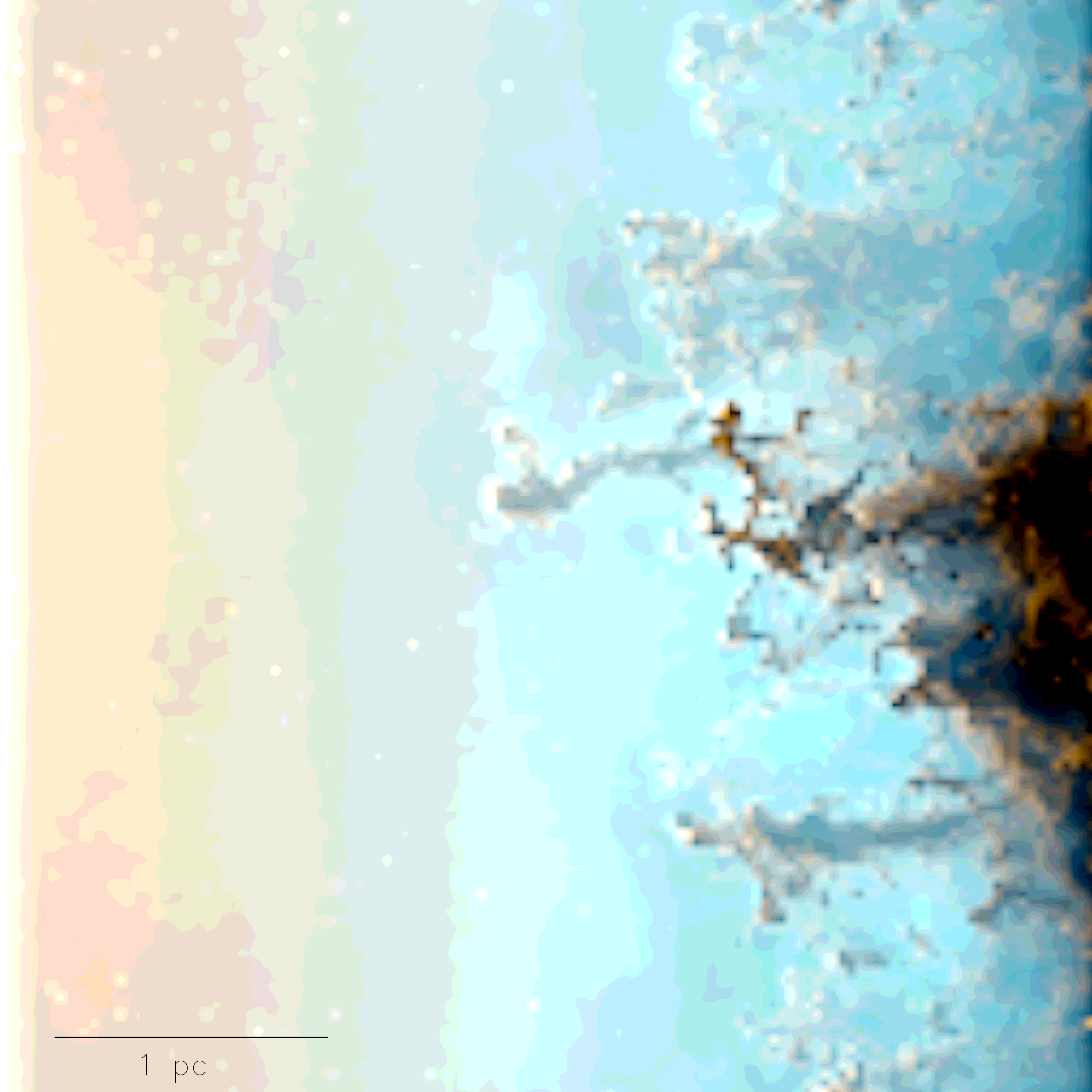
Figure 9: False colour composite image of the DiVINE simulation at t = 500kyr. Red = H$\alpha$, blue = $[$OIII$]\lambda\lambda$5007,4959 and green = combination.

Figure 1 shows the evolution of the surface density distribution for the standard iVINE run (upper panels) and the DiVINE run (lower panels). The figure suggests that the heating of low density gas by the diffuse field in the shadow regions results in a clumpier medium at late times. Comparison of volume density slices, like those shown at t = 500kyr in Figure 8, further highlight that a clear effect of the inclusion of the diffuse field is that the pillars are eroded from the back, promoting the detachment of clumps. This effect is less visible in integrated surface density maps as those shown in Figure 1.

Sim	$M$	$\bar{\rho}_{\mathrm{p}}$	$\bar{\Sigma}$	$\sigma$	$\bar{v}_{\mathrm{x}}$
	$[{\rm M}_{\odot}]$	$[{\thinspace m_{\mathrm{p}}\thinspace\mathrm{cm}^{-3}}]$	$[\mathrm{gcm}^{-2}]$	$[{\thinspace\mathrm{km}\thinspace\mathrm{s}^{-1}}]$	$[{\thinspace\mathrm{km}\thinspace\mathrm{s}^{-1}}]$
G09b	$12.6$	$4.56\times 10^{4}$	$1.52\times 10^{-3}$	$1.1\pm 0.7$	$4.8\pm 0.9$
DiVINE	$12.0$	$6.33\times 10^{4}$	$1.89\times 10^{-3}$	$0.9\pm 0.5$	$4.2\pm 0.8$

Table 1: Comparison of DiVINE and iVINE at t =500 kyr. Listed are the mass, mean density, mean surface density, velocity dispersion and the x-velocity away from the source of the most prominent structure. As the structure is not homogeneous we also include the standard deviation across the structure for both velocities.

The detailed comparison of the main structure obtained with DiVINE to the one obtained in G09b is given in Table 1. The regions compared are marked by the white boundaries drawn on the left hand panels of Figure 1. It is interesting to see that the total mass is not strongly affected. However, the DiVINE structure is denser and spatially thinner. The higher density leads to a slower motion away from the ionising source. By tracing the particles backwards in time we are able to determine that 75% of the material of the pillar in G09b ends up inside the pillar in DiVINE as well. Another effect of the higher density is enhanced triggered star formation. At $t=500$ kyr the star formation is still identical to G09b. The first star forms in the tip of the secondary pillar, at the same location and with similar properties as before. After that the star formation is different. A second star forms in DiVINE at the tip of the primary pillar after $t\approx 525$ kyr, while it forms much later in the G09b simulation (at $t\approx 735$ kyr).

Altogether the overall evolution is similar and the formation of structures is still governed by the initial turbulence, especially in high density regions, which are only weakly effected by diffuse radiation. However, small-scale dynamics and especially the triggered star formation change due to the inclusion of diffuse radiation.

We have also considered the observational appearance of such clumpy structures in typical narrow band filters, by computing the H$\alpha$ and $[$OIII$]\lambda\lambda$5007,4659 line emission and producing a false colours image along a line of sight parallel to the z-axis. We used the interstellar extinction curve of Weingartner & Draine (2001) for a Milky Way size distribution for R_V=3.1, with C/H = b_C = 60 ppm in log-normal size distributions, but renormalised by a factor 0.93. This grain model is considered to be appropriate for the typical diffuse HI cloud in the Milky Way. The result is shown in Figure 9, which shows ’pillar-like’ as well as ’horse-head-like’ structures very much resembling the famous Hubble Space Telescope images. Hence, even though, the structures are mostly detached from the parent cloud, the appearance is still that of coherent pillars.

5.3 Photoionisation-driven Turbulence

G09b found that turbulence on small scales could be sustained by the ionising radiation. We have revisited this question using the results obtained from DiVINE and we confirm the general conclusion that turbulence is driven by ionising radiation. A comparison of the iVINE and DiVINE turbulence spectra can be seen in Figure 10, where we plot the specific energy as a function of wave number (large wave numbers = small spatial scale) for the original control run with no ionising radiation presented by G09b (dotted lines), G09b’s standard iVINE run (dashed lines) and the DiVINE run presented in this work (solid lines). The efficiency of the driving is slightly reduced in the DiVINE calculations. We ascribe this effect to the higher compression of the cold gas due to the existence of the diffuse phase. The cold gas therefore experiences more shocks initially and is constrained more tightly, leading to lower turbulent motions.

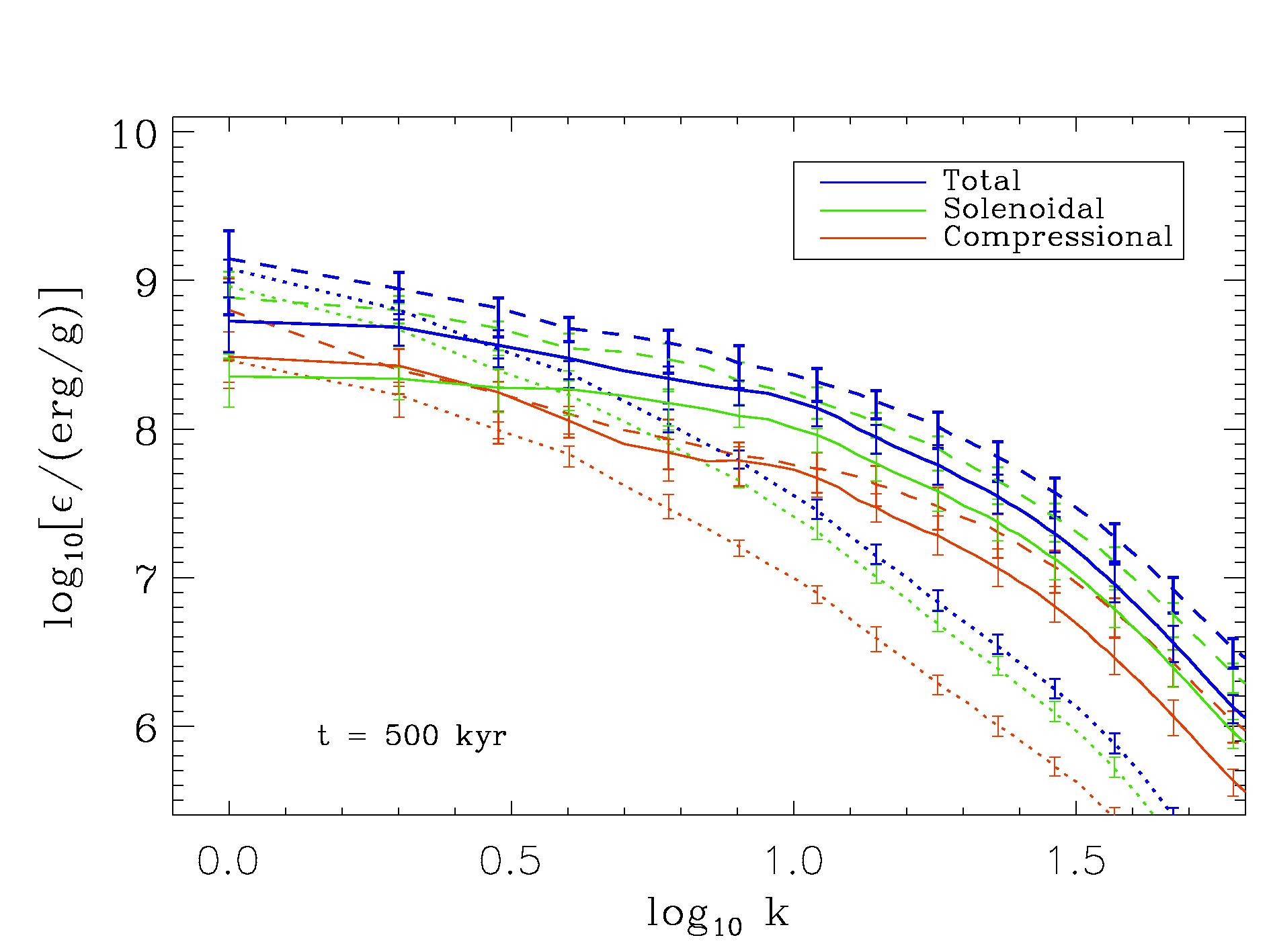
Figure 10: Specific energy as a function of wave number. Dotted lines: VINE run with no ionisation; solid lines: iVINE run; dashed lines DiVINE run

6 Conclusions

We have presented a detailed comparison of the ionisation and temperature structure for a turbulent ISM simulation performed with the SPH+ionisation code iVINE (Gritschneder et al 2009a,b, 2010) against the solution obtained with the photoionisation code MOCASSIN for snapshots of the density distribution. iVINE treats hydrodynamics, gravitational forces and ionisation simultaneously. The ionisation is calculated by making use of the ’on-the-spot’ (OTS) approximation. The MOCASSIN code (Ercolano et al 2003, 2005, 2008a) is fully three-dimensional and includes an exact treatment for the frequency resolved transfer of both the stellar (direct) and diffuse radiation fields. MOCASSIN includes all the microphysical processes that dominate the thermal and ionisation balance of the ionised gas, providing realistic temperature and ionisation distributions.

Our tests show that iVINE and MOCASSIN agree very well on the global properties of the region (i.e. total ionised mass fraction and location of the main ionisation front), but we note discrepancies in the temperature structure, particularly in the shadow regions. These tend to be cold and neutral in the iVINE plane-parallel stellar-field-only prescription , while MOCASSIN obtains a range of ionisation levels and temperatures that can be very crudely described as a function of density.

We have developed a computationally inexpensive strategy to include the thermal effects of the diffuse field, as well as accounting for environmental variables, such as gas metallicity and stellar spectra hardness. The method relies on the identification of the shadow region via simple criteria and application of a temperature parameterisation that was obtained a-priori using MOCASSIN. The method can be readily extended to other hydrodynamical codes (both SPH and grid-based).

We evaluate the effects of diffuse fields by comparing runs with the standard iVINE and the diffuse field implementation DiVINE. In agreement with previous studies (Raga et al 2009), we find that the overall qualitative behaviour of the system (i.e. the formation of what appear to be pillar like structures) is similar in the two runs. Nevertheless our models demonstrate that the diffuse field has important quantitative effects on the hydrodynamical evolution of the irradiated ISM. In particular we note that DiVINE predicts denser and less coherent structures which are much less attached to the parental cloud. This is due to the higher compression of the cold structures by the diffusively heated material inside the pillars trunks. Triggered star formation is promoted by this effect to a much earlier time. The compression also affects the turbulence spectrum of the system. We confirm the driving of turbulence by the ionising radiation, but with a slightly reduced efficiency compared to previous calculations with iVINE using the OTS approximation.

7 Acknowledgments

We thank Will Henney and Nate Bastian for useful discussion. We thank the referee for a constructive report that helped us improve the clarity of our paper. MG acknowledges additional funding by the China National Postdoc Fund Grant No. 20100470108 and the National Science Foundation of China Grant No. 11003001. Calculations presented here were partially using the University of Exeter Supercomputer, the KIAA Computational Cluster and the University of Munich SGI Altix 3700 Bx2 supercomputer that was partly funded by the DFG cluster of excellence ’Origin and Structure of the Universe’.

References

- Altay et al. (2008) Altay, G., Croft, R. A. C., & Pelupessy, I. 2008, MNRAS, 386, 1931
- Andrews et al. (2010) Andrews, J. E., et al. 2010, ApJ, 715, 541
- Bertoldi (1989) Bertoldi, F. 1989, ApJ, 346, 735
- Bisbas (2009) Bisbas, T.G., Wunsch, R., Whitworth, A. P., Hubber, D. A. 2009, A&A, 497, 649
- Dale et al. (2005) Dale, J. E., Bonnell, I. A., Clarke, C. J., & Bate, M. R. 2005, MNRAS, 358, 291
- Dale et al. (2007) Dale, J. E., Ercolano, B., & Clarke, C. J. 2007, MNRAS, 382, 1759
- Elmegreen et al. (1995) Elmegreen, B. G., Kimura, T., & Tosa, M. 1995, ApJ, 451, 675
- Ercolano et al. (2003) Ercolano, B., Barlow, M. J., Storey, P. J., & Liu, X.-W. 2003, MNRAS, 340, 1136
- Ercolano et al. (2004) Ercolano, B., Wesson, R., Zhang, Y., Barlow, M. J., De Marco, O., Rauch, T., & Liu, X.-W. 2004, MNRAS, 354, 558
- Ercolano et al. (2007) Ercolano, B., Bastian, N., & Stasińska, G. 2007, MNRAS, 379, 945
- Ercolano et al. (2007) Ercolano, B., Barlow, M. J., & Sugerman, B. E. K. 2007, MNRAS, 375, 753
- Ercolano et al. (2008) Ercolano, B., Drake, J. J., Raymond, J. C., & Clarke, C. C. 2008b, ApJ, 688, 398
- Ercolano et al. (2009) Ercolano, B., Clarke, C. J., & Drake, J. J. 2009, ApJ, 699, 1639
- Ercolano et al. (2005) Ercolano, B., Barlow,M. J., & Storey, P. J. 2005, MNRAS, 362, 1038
- Ercolano & Storey (2006) Ercolano, B., & Storey, P. J. 2006, MNRAS, 372, 1875
- Ercolano et al. (2008a) Ercolano, B., Young, P. R., Drake, J. J., & Raymond, J. C. 2008, ApJS, 175, 5345, 165
- Garcia-Segura & Franco (1996) Garcia-Segura, G., & Franco, J. 1996, ApJ, 469, 171
- Goodwin & Bastian (2006) Goodwin, S. P., & Bastian, N. 2006, MNRAS, 373, 752
- Gritschneder et al. (2009) Gritschneder, M., Naab, T., Walch, S., Burkert, A., & Heitsch, F. 2009b, ApJL, 694, L26
- Gritschneder et al. (2009) Gritschneder, M., Naab, T., Burkert, A., Walch, S., Heitsch, F., & Wetzstein, M. 2009a, MNRAS, 393, 21
- Gritschneder et al. (2010) Gritschneder, M., Burkert, A., Naab, T., & Walch, S. 2010, ApJ, 723, 971