Atmospheric parameter determination for massive stars via non-LTE spectrum analysis

Abstract

We describe a self-consistent spectrum analysis technique employing non-LTE line formation, which allows precise atmospheric parameters of massive stars to be derived: 1$\sigma$-uncertainties as low as $\sim$1% in effective temperature and $\sim$0.05–0.10 dex in surface gravity can be achieved. Special emphasis is given to the minimisation of the main sources of systematic errors in the atmospheric model computation, the observed spectra and the quantitative spectral analysis. Examples of applications are discussed for OB-type stars near the main sequence and their evolved progeny, the BA-type supergiants, covering masses of $\sim$8 to 25 M_⊙ and a range in effective temperature from $\sim$8 000 to 35 000 K. Relaxing the assumption of local thermodynamic equilibrium in stellar spectral synthesis has been shown to be decisive for improving the accuracy of quantitative analyses. Despite the present examples, which concentrate on hot, massive stars, the same philosophy can be applied to line-formation calculations for all types of stars, including cooler objects like the Sun, once the underlying stellar atmospheric physics is reproduced consistently.

1 Introduction

Many fields of contemporary astrophysics require a highly-precise determination of basic stellar parameters. A prime example is the investigation of stellar structure and evolution, where asteroseismology has opened up a window to study the governing physical processes in detail (e.g. Aerts et al. [2008]). Other examples are observational constraints on planet-formation theories by analyses of planet host stars (e.g. Neves et al. [2009]). Predictions of super-/hyper–nova models may be tested via analyses of secondary stars in low-mass X-ray binaries (e.g. González Hernández et al. [2008]) and (hyper-)runaway stars (Przybilla et al. [2008b]). Tight constraints on Galactochemical evolution theories may be derived using stars as tracers of the variation of chemical composition with time and location in the Galactic disk (e.g. Fuhrmann [2008]; Przybilla [2008]).

Precise stellar parameter determinations are decisive in describing the stellar atmospheric structure correctly, i.e. the temperature gradient and density stratification. This is crucial for the regions where the continuum and spectral lines of interest are formed. A fundamental problem is that a direct determination of stellar parameters is usually not possible. Quantitative spectral analysis has to rely on the comparison of synthetic spectra with observation, which in turn guides computations of improved models. In principle, this requires an iterative approach. In practice, however, approximate methods for the parameter determination are favoured on most occasions to shorten the process, by e.g. use of photometric indicators or comparison with prescribed (and thus necessarily limited) grids of models. Unfortunately, the gain in efficiency is often accompanied by a loss in accuracy.

Quantitative spectroscopy is highly prone to systematic errors. The analysis methodology, the quality of the observed spectra and the details of the assumptions made in the modelling, when taken together, determine the accuracy of a work. In particular, relaxing the assumption of local thermodynamic equilibrium (LTE) for the spectrum synthesis is crucial for improving the accuracy of stellar analyses.

In what follows we describe the basic requirements for a highly accurate determination of stellar atmospheric parameters by utilising all available lines of hydrogen and helium, plus multiple metal ionization equilibria, in non-LTE. We concentrate on OB-type stars near the main sequence and on their evolved progeny, BA-type supergiants. The stellar mass range between $\sim$8 and 25 M_⊙ is covered for effective temperatures from $\sim$8000 to 35 000 K. The models and analysis technique have been developed and thoroughly tested during the past years (Przybilla et al. [2006], PBBK06 henceforth; Nieva & Przybilla [2007, 2008], NP07/NP08; Przybilla, Nieva & Butler [2008c], PNB08). One should keep in mind that the same philosophy can, in principle, be applied to any type of star once the underlying stellar atmospheric physics is reproduced consistently.

We start with an overview of requirements on atmospheric models, the spectrum synthesis and the quality of observed spectra for a reliable quantitative analysis (Sects. 2 & 3). Then, a self-consistent spectrum analysis technique is described (Sect. 4). Concrete examples of stellar parameter determinations via non-LTE spectral analyses are discussed (Sect. 5). Finally, common sources of systematic error are briefly addressed (Sect. 6).

2 Model Requirements for the Spectral Analysis

An implicit requirement for high-precision quantitative spectrum analysis is the availability of model atmosphere and line-formation codes that account for all physics relevant to the objects of interest. All assumptions/approximations made to simplify the modelling need to be tested thoroughly to avoid fundamental sources of systematic effects in the analysis. Familiarity with the codes and the physics behind them are essential for successful work.

On the microscopic scale, the thermodynamic state of the plasma in a stellar atmosphere is determined by two competitive processes. Collisions act to establish detailed equilibrium locally, while radiative processes are non-local in character, thus driving the plasma out of detailed equilibrium. Local thermodynamic equilibrium is established only when either collisions dominate or the radiation field is isotropic and Planckian. Such conditions prevail to a good approximation deep in stellar atmospheres, but the strict validity of LTE can not be assumed for the observable layers. Instead, statistical equilibrium is established. The non-linear interdependency of radiation field and level populations is the essence of the non-LTE problem that in principle needs to be solved.

Nevertheless, stellar atmospheres are described well by the condition of LTE for many practical applications. In such a case non-LTE line formation assuming a LTE model atmosphere is sufficient to produce the synthetic spectra required for the comparison with observation.

The calculation of reliable occupation numbers for the energy levels involved in the transitions to be investigated is a prerequisite for an accurate analysis of spectra. Good agreement between model spectra and observation can be achieved when the following conditions are simultaneously fulfilled in the non-LTE computations: 1) the local temperatures and particle densities, i.e. the atmospheric structure, are accurately known, 2) the radiation field is realistic, 3) all relevant radiative and collisional processes are taken into account, and 4) high-quality atomic data are available.

Items 1) and 2) require a realistic physical model of the stellar atmosphere and thus an accurate atmospheric parameter determination. This will be the central topic here. Items 3) and 4) are related to the model atoms for the non-LTE calculations, hence a careful construction of comprehensive and robust model atoms is also required (see Przybilla, this volume). Shortcomings in any of the four conditions result in increased uncertainties of the analysis.

2.1 Models and Codes

Here we briefly recall the models and codes that provide the basis for the examples discussed in Sect. 5. We use a hybrid approach for the non-LTE line-formation computations. These are based on line-blanketed plane-parallel, homogeneous and hydrostatic LTE model atmospheres calculated with Atlas9 (Kurucz [1993b]). Line blanketing is realised via consideration of Opacity Distribution Functions (ODFs, Kurucz [1993a]), where the too high iron abundance originally used by Kurucz is compensated by ODFs with an appropriately reduced metallicity. This allows to approach modern values for the solar abundance (e.g. Asplund et al. [2005]), as iron contributes $\sim$50% of the line opacity. Alternatively, Atlas12 (Kurucz [1996]) is used for models with abundance peculiarities, allowing for opacity sampling. The model atmospheres are held fixed in the following non-LTE calculations.

Non-LTE level populations and synthetic spectra are computed with recent versions of Detail and Surface (Giddings [1981]; Butler & Giddings [1985]; both updated by K. Butler). Detail solves the coupled radiative transfer and statistical equilibrium equations employing the Accelerated Lambda Iteration scheme of Rybicki & Hummer ([1991]). This allows even complex ions to be treated in a realistic way. Synthetic spectra based on the resulting non-LTE populations are computed with Surface, using refined line-broadening data.

Detailed tests have shown that this hybrid non-LTE approach is consistent with full non-LTE calculations, but faster, for our cases of interest, BA-type supergiants (PBBK06) and OB-type dwarfs and giants (NP07). It also allows comprehensive model atoms to be employed. This can provide crucial improvements over full non-LTE calculations, which are necessarily based on simplified model atoms. An overview of model atoms adopted for our purposes is given in PBBK06 and PNB08.

3 Requirements on Observed Spectra

The advent of high-resolution spectrographs with large wavelength coverage, large telescopes and automated data reduction pipelines facilitates relatively easy access to high-quality spectra. However, some issues remain that introduce systematic errors into the quantitative analysis.

Continuum normalisation is one of the important issues, typically not achieved in a satisfactory way for echelle spectra with available data reduction pipelines alone. Cross-checks with lower-resolution long-slit spectra are recommended. A customised data reduction for order merging and rectification (see e.g. Hensberge [2007]) becomes often necessary when broad spectral features, like the hydrogen Balmer lines, are to be analysed. Uncertainties in the normalisation can lead to erroneous parameters from Balmer line analysis, such as for effective temperature for the later-type stars or surface gravity for early-type stars.

The modelling and analysis techniques should be tested on slowly-rotating stars of similar spectral type as the objects of interest. High-resolution and high-S/N spectra of such ‘standard stars’ are required to identify line blends. These may go unnoticed at lower spectral resolution or at higher rotational velocities, affecting analyses with incomplete linelists. Spectra of rapidly rotating stars are challenging, since rotational smearing can merge closely-spaced lines into a ‘pseudo-continuum’ below the true continuum. Line strengths may therefore be systematically underestimated. Full spectrum synthesis can facilitate an analysis, if continuum windows are found. The signal-to-noise (S/N) ratio can become one of the main sources of systematics, making continuum-definition difficult and weak lines inaccessible. Severe limitations to the quality of line fits may be imposed by low S/N. Some contribution of the observational material to the total uncertainty budget for stellar parameters and elemental abundances can be expected. However, well-selected targets and careful data acquisition and reduction can help to avoid unnecessary systematics (see Sect. 6 for more examples).

Figure 1: Schematic diagram of a self-consistent spectral analysis methodology. Note the iterative nature of the procedure. Numerous sources of systematic error need to be eliminated in every aspect of the process to achieve high accuracy. Spectral indicators for the quantitative analysis depend on the type of star.

4 Self-Consistent Spectral Analysis

Here we discuss our recommended spectrum analysis technique. Well-known concepts are assembled into a procedure that allows multiple stellar parameter indicators to be brought into agreement simultaneously. In combination with a determination of element abundances this facilitates the observation to be reproduced with a high degree of realism. The method works best when all lines of the Balmer series, the helium lines and many transitions of the metals are utilised. Spectral coverage at near-IR wavelengths is an asset. The method is organised as an iterative procedure, as sketched in Fig. 1.

Figure 2: Simultaneous fits to most observable hydrogen and helium lines in the optical spectrum of $\tau$ Sco (B0.2 V). Note that the He i/ii ionization balance is established. The only exception is the strong He ii $\lambda$4686 Å line which is affected by a weak stellar wind that is not accounted for in our calculations. From NP07.

Figure 3: Simultaneous fits to most observable carbon lines in the optical spectrum of $\tau$ Sco (B0.2 V). Every line fit adopts a slightly different abundance value, resulting in a 1$\sigma$ statistical uncertainty of 0.12 dex from the line-to-line scatter. The C ii/iii/iv ionization equilibrium is reproduced within these constraints. From NP08.

Figure 4: Non-LTE (filled symbols) and LTE (open symbols) carbon abundances derived from line profile fits to individual lines of six early B-type stars in the solar neighbourhood. Single (circles), double (diamonds) and triple-ionized (triangles) carbon lines are analysed. Note that non-LTE abundances show a lower scatter than the LTE results. The carbon ionization equilibrium is reproduced consistently in non-LTE. From NP08.

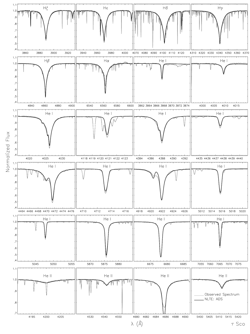
Good initial estimates for effective temperature, $T_{\mathrm{eff}}$, surface gravity, $\log g$, He abundance, $y$, microturbulent velocity, $\xi$, and metallicity, [M/H] (elemental abundances, $\varepsilon$(X)) are crucial to avoid many iteration cycles. Standard methods like photometric calibrations (see e.g. Smalley [2005]) plus estimates for the remaining quantities can be employed to gain initial approximations to start individualised calculations. Also, ‘secondary’ parameters like $\xi$ or $y$ have to be treated consistently in all steps of the computations to avoid the introduction of systematic errors. The comparison of the resulting synthetic spectrum with the observed spectrum gives indications as to how the input parameters should be changed to improve the next iteration. Alternatively, and more efficiently, pre-computed model grids may be utilised to perform line fits with a least-square algorithm (e.g. Fitprof, Napiwotzki [1999]). Parameter estimates are obtained from a $\chi^{2}$-minimisation. The first aim is to reproduce the observed hydrogen and helium spectra (see e.g. Fig. 2), the two elements constituting the bulk of the stellar material. Usually, reasonable values for $T_{\mathrm{eff}}$, $\log g$ and $y$ may be obtained for early-type stars. An advantage for the practical work is that the Stark-broadened hydrogen and helium lines are not highly sensitive to microturbulence and metallicity, except close to the Eddington limit (see Sect. 6).

Figure 5: Effective temperature determination for the LMC star NGC 2004-D15 via the silicon ionization equilibrium. The Si iii lines are strong, hence the derived silicon abundance depends on microturbulent velocity, $\xi$, while lines of the other two ions are less-sensitive to the choice of $\xi$ because of their weakness. Different $T_{\mathrm{eff}}$ is derived from Si ii/iii and Si iii/iv for ill-chosen $\xi$, e.g. an overestimation of $\xi$ by 7 km s^-1 gives $\Delta T_{\mathrm{eff}}$ $\approx$ 2000 K. The Si ii/iii/iv ionization equilibrium is established only for the correct $\xi$. From Nieva (2007).

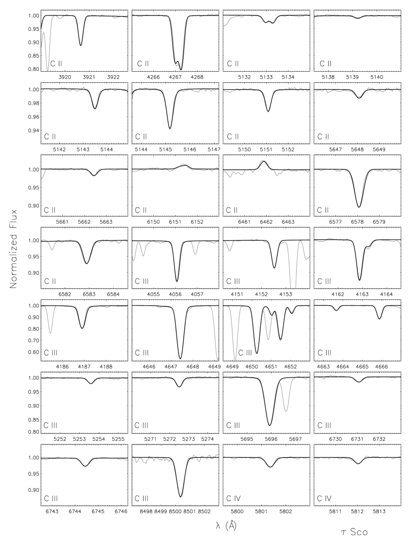
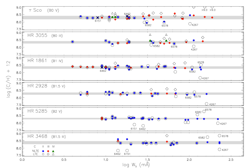
When a good fit to the H and He lines is achieved – $T_{\mathrm{eff}}$ and $\log g$ should be accurate to better than about 5% and 0.1–0.2 dex, respectively – the procedure commences to consider metal lines. Ionization equilibria, i.e. the requirement that lines from different ions of an element have to indicate the same elemental abundance, facilitate a fine-tuning of the previously derived parameters. Elements that show lines of three ionization stages in the spectrum are most valuable as they provide simultaneous constraints on both $T_{\mathrm{eff}}$ and $\log g$. Examples are C ii/iii/iv (Figs. 3 and 4) or Si ii/iii/iv in early B-type stars (Fig. 5). Typically, however, lines from only two ionization stages of an element are present in the spectrum, allowing only to constrain combinations of $T_{\mathrm{eff}}$ and $\log g$. Another indicator is then required for the parameter determination, e.g. the previously analysed H/He lines, or a second ionization equilibrium. We recommend the use of multiple ionization equilibria for the parameter determination as the redundancy of information helps to minimise systematics. Iron ionization equilibria are in particular useful as they put good constraints also on metallicity, [M/H] $\simeq$ [Fe/H].

Simultaneously, the microturbulent velocity needs to be constrained to values more accurate than the initial estimates at this stage. This is done by plotting abundances from the line analysis versus equivalent width $W_{\lambda}$ (see Fig. 4 for final results). A slope in the results indicates that the microturbulent velocity has to be adjusted. But there is much more to gain from such a plot: an offset of abundances from two ions indicates that the $T_{\mathrm{eff}}$/$\log g$ combination requires some fine-tuning. An excessive scatter in abundances points to remaining inconsistencies, e.g. with basic model assumptions (LTE in Fig. 4) or with the model atom.

The importance of a simultaneous determination of microturbulent velocity with other parameters – which is facilitated only iteratively – is shown in Fig. 5. This visualises the dependency of the resulting $T_{\mathrm{eff}}$ to the adopted value of $\xi$ when only one ionization equilibrium of silicon is considered, i.e. Si ii/iii or Si iii/iv. Different values are indicated for an ill-chosen microturbulent velocity. The problem can be solved via use of multiple ionization equilibria, e.g. by bringing Si ii/iii/iv simultaneously into agreement, and by considering also other elements as explained above. The goal is to derive the same value of $T_{\mathrm{eff}}$, $\log\,g$ and $\xi$ from all hydrogen, helium and the metal lines ($y$ may need to be adjusted only slightly at this stage).

Abundance analyses for elements not considered so far finalise the metallicity derivation. Usually, this brings no surprises for the stellar parameter determination. Exceptions can be chemically-peculiar stars, where our procedure is also useful (Przybilla et al. [2008a]) but more iteration steps can be required.

The final set of parameters has high precision and high accuracy. Absolute values of $T_{\mathrm{eff}}$ and $\log\,g$ show residual uncertainties as low as $\sim$1% and 0.05–0.10 dex, respectively, and for absolute elemental abundances an rms scatter of $\sim$10–20%. Remaining major sources of systematic error can essentially be excluded after bringing so many observational constraints into agreement. A self-consistent treatment of ‘secondary’ parameters such as $y$, [M/H] and $\xi$ throughout the entire process, from the atmospheric structure to the line-profile calculation is decisive for achieving this. Non-LTE ionization equilibria are sensitive to even small details of the calculations, so turning this sensitivity into a high-precision tool requires avoidance of any inconsistencies. We will resume the discussion on systematics in Sect. 6.

A limitation for the practical work is imposed by the iterative approach, the method is time-consuming. It is not feasible at the present time to analyse large samples of spectra efficiently. There are several ideas as to how to speed up the process, e.g. by analysis of a restricted but well-selected sample of spectral lines, which has to cover a variety of weak to strong lines of multiplets from the different spin systems of an ion. The full line sample is then analysed only in the final step. Extensive use of grids of non-LTE model spectra for metals with automatised line-fitting algorithms will play a crucial rôle in speeding-up the method, but require considerable computational resources to sample the multi-dimensional parameter space ($T_{\mathrm{eff}}$, $\log\,g$, $\xi$, $y$, [M/H] and abundances) properly. Nevertheless, we are confident that the analysis methodology will be applicable to high-precision studies of larger samples of stars in the near future.

5 Examples of Quantitative Analyses

O and B-type main-sequence and giant stars, and their evolved progeny, the B and A-type supergiants, constitute the objects with the simplest photospheric physics among the massive stars. They are unaffected by strong stellar winds like the hotter and more luminous stars or by convection and chromospheres like the cool stars. In order to use their full potential as tracers of stellar and galactochemical evolution (Przybilla [2008]) improvements in the quantitative analysis had to be implemented with respect to previous work. Comprehensive and robust model atoms for non-LTE line-formation calculations were constructed. In parallel, the self-consistent analysis technique described in Sect. 4 was implemented. Here we discuss some practical aspects from the use of the recommended analysis technique, giving special emphasis on the impact of non-LTE effects on both the analysis procedure and the results. An adaptation of the technique for the analysis of other types of stars could be done by analogy.

Figure 6: Example of systematic errors in carbon abundances caused by atmospheric parameter variations in a B0 III star. The offsets in parameters (values are indicated in the lower left corner of each panel) are averaged discrepancies for studies using standard analysis techniques. Incorrect parameters prevent consistent C ii/iii/iv abundances to be derived. Parameters determined from the carbon ionization equilibrium (NP08) were recently confirmed by other metal ionization equilibria (PNB08). ¿From NP08.

Table 1: Systematic errors in carbon abundances (in dex) from individual lines caused by atmospheric parameter variations and the assumption of LTE for line-formation calculations in the B0 III star HR 3055 ($T_{\mathrm{eff}}$ $=$ 31 200$\pm$300 K; $\log g$ $=$ 3.95$\pm$0.05; $\xi$ $=$ 8$\pm$2 km s^-1).

$$\footnotesize{\begin{array}[]{lcccccccc}\cr\hline\cr\mathrm{Ion}&\lambda&W_{\lambda}&\varepsilon(\mathrm{C})_{\mathrm{NLTE}}&\Delta T_{\mathrm{eff}}&\Delta\log\,g&\Delta\,\xi&\mathrm{LTE}\\ &\mathrm{(\AA)}&\mathrm{(m{\AA})}&&-2000\,\mathrm{K}&+0.2\,\mathrm{dex}&+5\,\mathrm{km\,s}^{-1}&\\ \hline\cr\\[-5.69054pt] \mathrm{C}$\,{\sc ii}$&4267.2&113&8.46&-0.33&-0.11&-0.16&-0.40\\[-1.42262pt] &5133.3&19&8.34&-0.30&-0.10&~{}~{}0.00&~{}~{}0.00\\[-1.42262pt] &5143.4&10&8.44&-0.40&-0.05&~{}~{}0.00&~{}~{}0.00\\[-1.42262pt] &5145.2&19&8.36&-0.32&-0.09&-0.02&~{}~{}0.00\\[-1.42262pt] &5151.1&11&8.34&-0.30&-0.08&~{}~{}0.00&~{}~{}0.00\\[-1.42262pt] &5662.5&~{}4&8.37&-0.33&-0.13&~{}~{}0.00&~{}~{}0.00\\[-1.42262pt] &6578.0&66&8.24&-0.40&-0.15&-0.10&~{}~{}0.00\\[-1.42262pt] &6582.9&37&8.29&-0.30&+0.02&+0.05&+0.05\\[2.84526pt] \mathrm{C}$\,{\sc iii}$&4056.1&45&8.28&+0.21&+0.06&-0.04&+0.08\\[-1.42262pt] &4162.9&58&8.29&+0.28&+0.09&-0.03&+0.25\\[-1.42262pt] &4186.9&92&8.34&+0.35&+0.15&-0.08&+0.07\\[-1.42262pt] &4663.5&18&8.27&+0.22&+0.07&-0.03&+0.22\\[-1.42262pt] &4665.9&50&8.24&+0.26&+0.08&-0.08&+0.35\\[-1.42262pt] &5272.5&14&8.28&+0.16&+0.01&~{}~{}0.00&~{}~{}0.00\\[2.84526pt] \mathrm{C}$\,{\sc iv}$&5801.3&53&8.45&+1.06&+0.46&-0.03&+0.39\\[-1.42262pt] &5811.9&34&8.45&+1.06&+0.46&-0.03&+0.39\\[1.42262pt] \hline\cr\end{array}}$$

Let us summarise the spectroscopic indicators for the parameter determination:

• $T_{\mathrm{eff}}$: all available hydrogen and helium lines & ionization equilibria

• $\log g$: wings of all available hydrogen lines & ionization equilibria

• $y$: all available helium lines

• $\varepsilon\mathrm{(X)}$: a comprehensive set of metal lines

• $\xi$: metals with numerous lines of different strength, slope 0 in $\varepsilon\mathrm{(X)}$ vs. W_λ

• $v\sin i$ and $\zeta$: from metal line-profile fits

• $\mathrm{[M/H]}$: abundance analysis

We see that the analysis requires high-resolution spectra with a near-complete wavelength coverage in the optical and reliable continuum rectification, preferentially at high S/N. Additional constraints, when available, are recommended to be checked for consistency, like spectral energy distributions (SEDs) or highly sensitive spectral lines in the near-IR (Nieva et al. [2009]; Przybilla, this volume).

5.1 OB-type Main Sequence and Giant Stars

Spectral indicators for $T_{\mathrm{eff}}$ and $\log g$ in late-O and early-B main sequence and giant stars are the hydrogen and helium lines. In addition, several of the following ionization equilibria are used, depending on the temperature range: He i/ii, C ii/iii/iv, O i/ii, Ne i/ii, Si ii/iii/iv and Fe ii/iii. Simultaneous fits to most observable H, He and C lines in a FEROS spectrum are shown in Figs. 2 and 3. In a hot star like $\tau$ Sco practically all the H and He lines show marked non-LTE strengthening. Line cores as well as the wings are affected, see NP07 for details. The He i/ii and C ii/iii/iv ionization balance is established simultaneously in non-LTE. This is impossible to achieve assuming LTE because of the different sensitivity of the lines to non-LTE effects. In the case of hydrogen and helium a unique model is employed for all fits. For carbon, because of the higher sensitivity of the lines to the chemical abundance, every line fit employs a slightly different abundance value. The resulting non-LTE abundances for this element show a low rms scatter, and even more so for other stars (see Fig. 4).

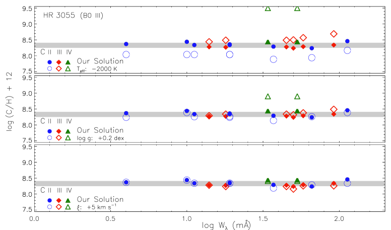
The effects of variations in $T_{\mathrm{eff}}$, $\log\,g$ and $\xi$ on carbon abundances from individual lines in a B0 III star are shown in Fig. 6. They have been quantified for representative lines in Table 1. The offsets in parameters are averaged discrepancies for studies using standard analysis techniques like photometric indicators. An offset in a parameter prevents consistent C ii/iii/iv ionization equilibrium to be achieved, even when the model atom is highly reliable. Displacements of the average abundances for the different ions occur in such a situation. This can introduce unnoticed systematics to abundance results whenever only one ion is studied for poorly-constrained stellar parameters. The effects are largest for $T_{\rm eff}$ variations and lowest for modifications of $\xi$, in particular for the weaker lines. Non-LTE effects can be the dominant factor for the abundance determination for some lines (e.g. C ii $\lambda$4267 Å or C iii $\lambda$4666 Å, see Table 1), but in many cases a reliable parameter determination is more important than accounting for deviations from LTE. Both non-LTE weakening and strengthening can occur for different lines of the same ion, and non-LTE effects may dominate even weak lines, contrary to common expectation. The best examples are the weak C ii $\lambda\lambda$6151 and 6462 Å emission lines (Fig. 3), which remain unexplained by LTE line formation.

Figure 7: $T_{\mathrm{eff}}$ and $\log g$ effects on magnesium and hydrogen lines, and the final solution of the parameter determination accounting also for the nitrogen ionization equilibrium and helium abundances in $\eta$ Leo, (A0 Ib). Upper left panel: Mg i lines are sensitive to $T_{\mathrm{eff}}$ and $\log g$ variations. Upper right panel: Mg ii lines are not sensitive to these parameters. Lower left panel: sensitivity of H$\delta$ to $T_{\mathrm{eff}}$ and $\log g$ variations. Lower right panel: final solution as the intersection of the different loci for the H lines and Mg and N ionization equilibria with parametrised He abundance in the $T_{\mathrm{eff}}$–$\log g$ plane. From PBBK06.

Figure 8: Determination of macroturbulent ($\zeta$) and projected equatorial rotation ($v\sin i$) velocities in $\eta$ Leo. The upper comparison between observation (thick) and spectrum synthesis (thin line, for finally derived mean abundances) takes into account $\zeta$ and $v\sin i$, while the lower comparison assumes a pure rotational profile. From PBBK06.

5.2 BA-type Supergiants

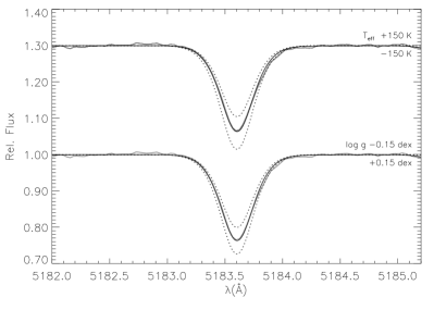
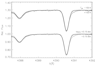
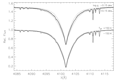
Spectral indicators for $T_{\mathrm{eff}}$ and $\log g$ in late-B and early-A supergiants are the Stark-broadened hydrogen lines and several non-LTE ionization equilibria. We utilise at least two of the following: C i/ii, N i/ii, O i/ii, Mg i/ii, Si ii/iii or S ii/iii. Examples for the (high) sensitivity of the Mg i/ii lines and a Balmer line in an A0 Ib supergiant to $T_{\mathrm{eff}}$/$\log g$ variations are shown in Fig. 7. Each indicator allows to construct a curve in the $T_{\mathrm{eff}}$–$\log g$ plane for which the observed features are reproduced well. Note that the helium abundance has to be varied accordingly in this process, i.e. the observed He i lines need to be reproduced simultaneously, as the atmospheric structure of such a luminous object reacts noticeably to changes of the mean molecular weight of the plasma. The intersection of all loci determines the final parameters (see Fig. 7).

Figure 9: Elemental abundances from individual spectral lines as a function of equivalent width, see the legend for symbol encoding. The grey bands cover the 1$\sigma$-uncertainty around the non-LTE averages. Proper non-LTE calculations reduce the line-to-line scatter and remove systematic trends. The same value for microturbulent velocity is adopted in all cases. From PBBK06.

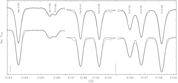
Detailed line-profile fits are much more powerful than analyses of equivalent widths (i.e. of only an integrated quantity). For line fitting, additional parameters need to be known, the projected equatorial rotational velocity, $v\sin i$, and the macroturbulent velocity, $\zeta$, which we determine within our spectrum synthesis approach. The rotational and macroturbulent broadening profiles are convolved with the synthetic spectrum, and $v\sin i$ and $\zeta$ are varied until the observed profiles are matched. This allows high accuracy of these parameters to be obtained. Both, regions with unblended or with blended lines are useful for the derivation (see Fig. 8). Alternatively, Gray’s Fourier transform technique may be employed (see e.g. Simón-Díaz & Herrero ([2007]) for applications to early-type stars).

Figure 9 is analogous to Fig. 4, but for different elements in an A0 Ib star. Besides indicating a proper choice of microturbulence, which is found to be the same for all elements from the non-LTE analysis, from slope zero of $\varepsilon$(X) vs. $W_{\lambda}$, also a match of the ionization equilibria (C i/ii, N i/ii and Mg i/ii) is found. Moreover, the comparison with LTE abundances shows that non-LTE effects are ubiquitous, i.e. they have to be accounted for in every step of the analysis. The non-LTE analysis finds homogeneous abundances from all lines in the element spectra, which show little scatter around the mean value (less than in LTE). Systematic trends of abundance with line-strength found in LTE, e.g. for N i or O i, are absent in non-LTE. In other cases, for S ii, Ti ii and Fe ii, the non-LTE abundances are systematically shifted relative to LTE. Contrary to common assumption significant non-LTE abundance corrections are found even in the weak-line limit. These can exceed a factor $\sim$2 for lines with $W_{\lambda}$ $<$ 10 mÅ, in particular for more luminous objects with amplified non-LTE effects. At the other extreme, for the strongest oxygen or nitrogen lines, abundance corrections can amount to a factor $\sim$50, or even more.

Figure 10: Global spectrum synthesis for HD 92207 (A0 Iae) resulting from the successful quantitative spectral analysis. From PBBK06.

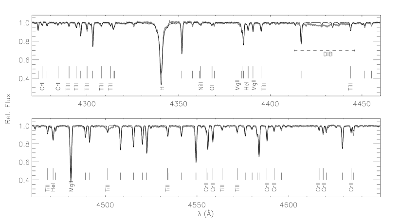
The fruit of such a comprehensive stellar parameter and abundance analysis is a synthetic spectrum, which should reproduce the observed spectrum. A comparison of model with observation is the final test. Very good agreement can indeed be obtained even for extreme objects, see Fig. 10. Note that a few discrepancies can remain, like those imposed by the presence of diffuse interstellar bands (DIBs).

6 Summary of Common Sources of Systematic Errors

Every step in the quantitative spectral analysis is susceptible to systematic errors. Here we briefly list the most common sources of systematics that affect the final uncertainties of stellar parameters and elemental abundances. We concentrate on systematics encountered in the study of massive stars and, when possible, give recipes for how to prevent them. The overview should be useful also for work on other types of stars, but can include additional complications, such as convection in cool stars or magnetic fields, which are beyond the scope of the present discussion.

Figure 11: Left panel: variations of the atmospheric temperature structure in response to changes of helium abundance (lower), and effects of metallicity (middle) and microturbulence (upper set of curves) on the atmospheric line blanketing. The comparison is made for stellar parameters matching those of an A0 Iae star. Only one parameter is modified at each time: $y$ = 0.089 (solar value, full line) and $y$ = 0.15 (dotted line); use of ODFs with $[$M/H$]$ = 0.0, $-$0.3, $-$0.7 and $-1.0$ dex (full, dotted, dashed, dashed-dotted lines); use of ODFs with $\xi$ = 8, 4 and 2 km s^-1 (full, dotted, dashed lines). For clarity, offsets by $+$1000 K and $+$2000 K have been applied to the middle and upper set of curves, respectively. In the inset, the formation region for weak lines is enlarged. Right panel: analogous to the left panel, but for the atmospheric electron density. From PBBK06.

Figure 12: Effects of varying atmospheric helium abundance (lower), metallicity (middle) and microturbulence (upper set of curves) on the profiles of diagnostic lines in an A0 Iae supergiant, using the models discussed in Fig. 11. Note that the line profile changes are due to the effects of modified mean molecular weight and line blanketing alone. Values of e.g. $T_{\rm eff}$, $\log g$ and the magnesium abundance remain unchanged. For clarity, offsets have been applied to the different sets of curves. ¿From PBBK06.

Model atmospheres and line formation. Atmospheric structures/SEDs computed with full non-LTE or hybrid non-LTE methods are equivalent for studies of unevolved OB-type stars (NP07) and BA-type supergiants (PBBK06). This is not a source of systematics for these cases, but this needs to be tested for other types of objects. Crucial for comparisons is that the same abundances are used in both approaches. Abundance values need to be checked explicitly for model comparisons, e.g. for ‘solar’ abundances, as the solar ‘standard’ has changed with time. Secondary parameters like helium abundance, microturbulent velocity and metallicity can affect atmospheric structures via their impact on the mean molecular weight or on line-blanketing/blocking effects. Examples of the effects to be expected on the structure of a loosely-bound atmosphere of a star close to the Eddington limit and on the resulting synthetic spectra are shown in Figs. 11 and 12, respectively. In such a case the effects are not negligible at all (see PBBK06 for a detailed discussion). These parameters need to be treated in a consistent way.
Line blocking. The presence of numerous lines in a spectrum affects the radiation field. The radiation is blocked within the lines, and redistributed into neighbouring continuum bands because of flux conservation. Typically, the flux in the UV, where many lines are present, is diminished and more radiation is emitted in the optical. Non-LTE line-formation calculations need to account for this line blocking effect, e.g. by using ODFs or opacity sampling techniques. The ‘softer’ radiation field yields less ionization, affecting all ionization equilibria.
Model atoms. Most model atoms for non-LTE calculations are based on input atomic data (ab-initio data and approximations) as available in the early 1990s. It is worthwhile to check for improvements on the modelling whenever new data becomes available. As an example, different carbon model atoms can yield discrepancies in abundance analyses up to 0.8 dex for strategic lines (NP08).
Line-broadening theory. Progress made on line-broadening theory has provided a wealth of detailed broadening parameters over the past years. Detailed tabulations like those of Stehlé & Hutcheon ([1999]) for the Stark-broadening of hydrogen line profiles should be favoured over simpler approximations for a reliable stellar parameter determination. For cool stars a detailed treatment of the broadening of spectral lines by neutral hydrogen collisions is highly important (e.g. Barklem et al. [2000a, 2000b]).
Composite spectra. Binary stars are common, and spectra of apparently single stars may turn out to be of composite nature. Light from the fainter, secondary star may not be accompanied by radial velocity variations for wide binaries, or for chance alignments of stars when observing dense fields. Standard analysis methods for single stars applied to a spectrum where the light from both stars is detected can give erroneous results throughout. Inspection of hydrogen or helium lines for asymmetries, or for the presence of (weak) features not fitting a star’s spectral type may be helpful to identify such cases. In addition, signatures like UV or IR excess should be checked in case of doubt.
Quality of spectra. Continuum normalisation and local continuum definition are major sources of systematics for the analysis of spectra with S/N $\leq$ 50. The abundance determination in stars rotating at intermediate velocities ($v\sin i\sim 50-150\,\mathrm{km\,s^{-1}}$) is already limited to 0.2–0.3 dex in accuracy at this S/N. Rapidly-rotating stars ($v\sin i>150\,\mathrm{km\,s^{-1}}$) or low-resolution spectra impose even more complications because metal line blends lower the actual continuum. Hence, the abundances can be systematically underestimated and the accuracy is typically limited to 0.3–0.4 dex (see Korn et al. [2005]).
Effective temperatures. $T_{\mathrm{eff}}$ estimated from photometry can differ by more than 10% (NP08) from that determined with a self-consistent spectroscopic method. Spectroscopic determinations via ionization equilibria are a powerful technique only when the model atoms are reliable. In addition, one ionization equilibrium alone does not provide accurate constraints because of dependencies on other variables (see Fig. 5 for the case of silicon) and consequences for carbon abundances in Fig. 6 and Table 1. Therefore, only the simultaneous use of multiple ionization equilibria provides a precise and accurate $T_{\mathrm{eff}}$ determination.
Surface gravity. The common use of only one Balmer line as $\log\,g$ indicator does not allow for consistency checks. Instead, all available H lines and in addition metal ionization equilibria should be considered for an accurate determination. Moreover, the neglect of non-LTE effects on the Balmer lines, as often found in the literature, can lead to systematic errors: increasing with $T_{\mathrm{eff}}$ up to $\sim$0.2 dex in $\log\,g$ around 35 000 K, see e.g. Table 1 for effects on the carbon analysis.

Figure 13: Theoretical line profiles for magnesium lines in $\eta$ Leo, assuming $\xi$ $=$ 10 km s^-1. The predictions differ when microturbulence is accounted for self-consistently in the statistical equilibrium and radiative transfer calculations (full line) and when it is considered only in the formal solution (dotted), which is the standard. From Przybilla et al. ([2001]).

Microturbulence. This quantity is often derived from lines of only one ion of one element (e.g. O ii in early-type stars) and in extreme cases from only one multiplet (e.g. Si iii $\lambda\lambda$4552–4574). Cross-checks with different species are mandatory when only a few lines are measurable (like in fast rotators) to avoid large uncertainties. Identical values for $\xi$ are expected to be obtained in a proper non-LTE analysis of different ions/chemical species, see Sect. 5.2. Microturbulent velocities in excess of the sound speed are suspicious. Often neglected is the effect of microturbulence on the radiative bound-bound transition rates in the non-LTE computations. The strengths of lines, their shape and their formation depth may be affected (see Fig. 13 for an example).
Spectral line selection. Abundances may depend on the selection of lines used in the analysis when the model atoms are not comprehensive: some multiplets may indicate systematically different abundances than others. Which lines should be trusted for the analysis? Comparison with other model atoms may help, some transitions may be found not to deviate from LTE. However, we recommend to investigate the reasons for such discrepancies, and implementation of improvements for the model atoms. In principle, all possible observed lines of an atom/ion should be analysed (see NP08 and PNB08).
Non-LTE ‘corrections’. Non-LTE effects cannot be easily predicted. They affect different lines in different ways (see Fig. 9). Non-LTE line strengthening or weakening can occur, or lines may turn out to be ‘in LTE’. Non-LTE effects are not restricted to the stronger lines alone. For different plasma conditions the non-LTE effects change, see Fig. 4. Hence, adding or subtracting fixed ‘non-LTE abundance corrections’ to LTE results may increase the systematics.
Macroturbulence. Macroturbulence is not considered in many studies. This is important for proper $v\sin i$ determinations, in particular for apparently slowly-rotating objects. An example is shown in Fig. 8, where a $v\sin i$ of zero is derived when macroturbulence is accounted for and $\sim$13 km s^-1 if it is not.

7 Conclusions

Highly-precise and accurate stellar parameters can be spectroscopically determined, with limiting uncertainties as low as $\sim$1% in $T_{\mathrm{eff}}$, $\sim$0.05–0.10 dex in $\log\,g$ and $\sim$10-20% in elemental abundances (rms scatter). A self-consistent spectral analysis methodology using non-LTE line formation was presented that allows this to be achieved when typical systematics are avoided. Of crucial importance is to simultaneously bring multiple spectroscopic indicators into agreement, which requires an iterative approach. The method is much more time-consuming than standard approaches for the stellar parameter determination, but it is worth the effort whenever highly-accurate observational constraints are required for astrophysical applications.

References

- [2008] Aerts, C., Christensen-Dalsgaard, J., Cunha, M. & Kurtz, D. W. 2008, Sol. Phys., 251, 3
- [2005] Asplund, M., Grevesse, N. & Sauval, A. J. 2005, in “Cosmic Abundances as Records of Stellar Evolution and Nucleosynthesis”, ed. T. G. Barnes III & F. N. Bash (ASP: San Francisco), p. 25
- [2000a] Barklem, P. S., Piskunov, N. & O’Mara, B. J. 2000a, A&AS, 142, 467
- [2000b] Barklem, P. S., Piskunov, N. & O’Mara, B. J. 2000b, A&A, 363, 1091
- [1985] Butler, K. & Giddings, J. R. 1985, in Newsletter of Analysis of Astronomical Spectra, No. 9, Univ. London
- [2008] Fuhrmann, K. 2008, MNRAS, 384, 173
- [1981] Giddings, J. R. 1981, Ph.D. Thesis, Univ. London
- [2008] González Hernández, J. I., Rebolo, R. & Israelian, G. 2008, A&A, 478, 203
- [2007] Hensberge, H. 2007, in “The Future of Photometric, Spectrophotometric and Polarimetric Standardization”, ed. C. Sterken (ASP: San Francisco), p. 275
- [2005] Korn, A. J., Nieva, M. F., Daflon, S. & Cunha, K. 2005, ApJ, 633, 899
- [1993a] Kurucz, R. L. 1993a, CD-ROM No. 2–12 (Cambridge, Mass.: SAO)
- [1993b] Kurucz, R. L. 1993b, CD-ROM No. 13 (Cambridge, Mass.: SAO)
- [1996] Kurucz, R. L. 1996, in “Model Atmospheres and Spectrum Synthesis”, ed. S. J. Adelman, F. Kupka & W. W. Weiss (ASP: San Francisco), p. 160
- [1978] Mihalas, D. 1978, Stellar Atmospheres, 2nd edition (San Francisco: Freeman)
- [1999] Napiwotzki, R. 1999, A&A, 350, 101
- [2009] Neves, V., Santos, N. C., Sousa, S. G., et al. 2009, A&A, 497, 563
- [2007] Nieva, M. F. 2007, Ph.D. Thesis, Univ. Erlangen-Nuremberg and Observatório Nacional Rio de Janeiro (Verkannten Verlag: Berlin)
- [2007] Nieva, M. F. & Przybilla, N. 2007, A&A, 467, 295 (NP07)
- [2008] Nieva, M. F. & Przybilla, N. 2008, A&A, 481, 199 (NP08)
- [2009] Nieva, M. F., Przybilla, N., Seifahrt, A., et al. 2009, in “Science with the VLT in the ELT era”, ed. A. Moorwood (Springer: Berlin), p. 499
- [2008] Przybilla, N. 2008, Rev. Mod. Astron., 20, 323
- [2001] Przybilla, N., Butler, K., Becker, S. R. & Kudritzki, R. P. 2001, A&A, 369, 1009
- [2006] Przybilla, N., Butler, K., Becker, S. R. & Kudritzki, R. P. 2006, A&A, 445, 1099 (PBBK06)
- [2008a] Przybilla, N., Nieva M. F., Tillich A., et al. 2008a, A&A, 488, L51
- [2008b] Przybilla, N., Nieva, M. F., Heber, U. & Butler, K. 2008b, ApJ, 684, L103
- [2008c] Przybilla, N., Nieva, M. F. & Butler, K. 2008c, ApJ, 688, L103 (PNB08)
- [1991] Rybicki, G. B. & Hummer, D. G. 1991, A&A, 245, 171
- [2007] Simón-Díaz, S. & Herrero, A. 2007, A&A, 468, 1063
- [2005] Smalley, B. 2005, Mem. Societa Astronomica Italiana Suppl., 8, 130
- [1999] Stehlé, C. & Hutcheon, R. 1999, A&AS, 140, 93