A New Hybrid N-Body-Coagulation Code for the Formation of Gas Giant Planets

Abstract

We describe an updated version of our hybrid $N$-body-coagulation code for planet formation. In addition to the features of our 2006–2008 code, our treatment now includes algorithms for the 1D evolution of the viscous disk, the accretion of small particles in planetary atmospheres, gas accretion onto massive cores, and the response of $N$-bodies to the gravitational potential of the gaseous disk and the swarm of planetesimals. To validate the N-body portion of the algorithm, we use a battery of tests in planetary dynamics. As a first application of the complete code, we consider the evolution of Pluto-mass planetesimals in a swarm of 0.1–1 cm pebbles. In a typical evolution time of 1–3 Myr, our calculations transform 0.01–0.1 $\rm M_{\odot}$ disks of gas and dust into planetary systems containing super-Earths, Saturns, and Jupiters. Low mass planets form more often than massive planets; disks with smaller $\alpha$ form more massive planets than disks with larger $\alpha$. For Jupiter-mass planets, masses of solid cores are 10–100 $\rm M_{\oplus}$.

1 INTRODUCTION

Gas giant planets form in gaseous disks surrounding young stars. In the ‘core accretion’ theory, collisions and mergers of solid planetesimals produce 1–10 $\rm M_{\oplus}$ (Earth mass) icy cores which rapidly accrete gas (e.g., Pollack et al., 1996; Alibert et al., 2005; Ida & Lin, 2005; Chabrier et al., 2007; Lissauer & Stevenson, 2007; Dodson-Robinson et al., 2008; D’Angelo et al., 2010). As the planets grow, viscous transport and photoevaporation also remove material from the disk (e.g., Alexander & Armitage, 2009; Owen et al., 2010). Eventually, these processes exhaust the disk, leaving behind a young planetary system.

Observations place many constraints on this theory. Although nearly all of the youngest stars are surrounded by massive disks of gas and dust, very few stars with ages of 3–10 Myr have dusty disks (e.g., Haisch, Lada, & Lada, 2001; Currie et al., 2009; Kennedy & Kenyon, 2009; Mamajek, 2009). Thus, gas giant planets must form in 1–3 Myr. Stars with ages of $\sim$ 1 Myr have typical disk masses of 0.001–0.1 $\rm M_{\odot}$ and disk radii of 10–200 AU (e.g., Andrews & Williams, 2005; Isella et al., 2009), setting the local environment where planets form. For stars with ages of $\sim$ 1 Gyr, the frequency of ice/gas giant planets around low mass stars is $\sim$ 20%–40% (Cumming et al., 2008; Gould et al., 2010). Although many known exoplanets are gas giants with masses comparable to Jupiter, lower mass planets outnumber Jupiters by factors of $\sim$ 10 (Mayor et al., 2009; Borucki et al., 2010; Gould et al., 2010; Holman et al., 2010; Howard et al., 2010).

Despite the complexity of the core accretion theory, clusters of computers are now capable of completing an end-to-end simulation of planet formation in an evolving gaseous disk. Our goal is to build this simulation and to test the core accretion theory. Over the past decade, we have developed a hybrid, multiannulus $N$-body–coagulation code for planet formation (Kenyon & Bromley, 2004a; Bromley & Kenyon, 2006; Kenyon & Bromley, 2008). The centerpieces of our approach are a multiannulus coagulation code – which treats the growth and dynamical evolution of small objects in 2D using a set of statistical algorithms – and an $N$-body code – which follows the 3D trajectories of massive objects orbiting a central star. With additional software to combine the two codes into a unified whole, we have considered the formation of terrestrial planets (Kenyon & Bromley, 2006) and Kuiper belt objects (Kenyon & Bromley, 2004c; Kenyon et al., 2008) around the Sun and the formation and evolution of debris disks around other stars (Kenyon & Bromley, 2004a, 2004b, 2008, 2010).

Treating the formation of gas giant planets with our 2008 code (Kenyon & Bromley, 2008) requires algorithms for additional physical processes. As described in §2, we added (i) a 1D solution for the evolution of a viscous disk on a grid extending from 0.2 AU to $10^{4}$ AU (Chambers, 2009; Alexander & Armitage, 2009), (ii) algorithms for accretion of small particles encountering a planetary atmosphere (Inaba & Ikoma, 2003) and for accretion of gas onto massive cores, (iii) a prescription for the evolution of the radius and luminosity of a gas giant planet accreting material from a disk, and (iv) new code to treat the gravitational potential of the gaseous disk and the swarm of planetesimals in the $N$-body code. Tests of these additions demonstrate that our complete code reproduces the simulations of viscous disks in Alexander & Armitage (2009), accretion rates for small particles in Inaba & Ikoma (2003) and for gas in D’Angelo et al. (2010), and the battery of $N$-body code tests from Bromley & Kenyon (2006). In §3, we show that our code also reproduces results for planets migrating through planetesimal disks (Hahn & Malhotra, 1999; Kirsh et al., 2009).

As a first application to gas giant planet formation, we consider whether ensembles of Pluto-mass cores embedded in gaseous disks with masses of 0.01–0.1 $\rm M_{\odot}$ can become gas giant planets. Our results in §4 demonstrate that a disk of Pluto-mass objects will not form gas giants in 10 Myr. However, a few Pluto-mass seeds embedded in a disk of 0.1–1 cm pebbles can evolve into a planetary system with super-Earths, Saturns, and Jupiters. If we neglect orbital migration, ice and gas giants form at semimajor axes of 1–100 AU on timescales of 1–3 Myr. Thus, these calculations match some of the observed properties of exoplanets without violating the constraints imposed by observations of gaseous disks around the youngest stars.

2 THE MODEL

2.1 Disk evolution

Disk evolution sets the context for our planet formation calculations. Viscous processes within the disk transport mass inwards onto the central star and angular momentum outwards into the surrounding molecular cloud. Heating from the central star modifies the temperature structure within the disk and removes material from the upper layers of the disk. All of these processes change disk structure on timescales comparable to the growth time for planetesimals. Thus, planets form in a rapidly evolving disk.

For a disk with surface density $\Sigma$ and viscosity $\nu$, conservation of angular momentum and energy leads to a non-linear diffusion equation for the time evolution of $\Sigma$ (e.g., Lynden-Bell & Pringle, 1974; Pringle, 1981),

$$\frac{\partial\Sigma}{\partial t}=3R^{-1}~{}\frac{\partial}{\partial R}~{}\left(R^{1/2}~{}\frac{\partial}{\partial R}~{}\{\nu\Sigma R^{1/2}\}\right)-\left(\frac{\partial\Sigma}{\partial t}\right)_{ext}~{},$$ (1)

where $R$ is the radial distance from the central star and $t$ is the time. The first term is the change in $\Sigma$ from viscous evolution; the second term is the change in $\Sigma$ from other processes such as photoevaporation (e.g., Alexander et al., 2006; Owen et al., 2010) or planet formation (e.g., Alexander & Armitage, 2009). The viscosity is $\nu=\alpha c_{s}H$, where $c_{s}$ is the sound speed, $H$ is the vertical scale height of the disk, and $\alpha$ is the viscosity parameter. The sound speed is $c_{s}^{2}=\gamma kT_{d}/\mu m_{H}$, where $\gamma$ is the ratio of specific heats, $k$ is Boltzman’s constant, $T_{d}$ is the midplane temperature of the disk, $\mu$ is the mean molecular weight, and $m_{H}$ is the mass of a hydrogen atom. The scale height of the disk is $H$ = $c_{s}\Omega^{-1}$, where $\Omega=GM_{\star}/R^{3}$ is the angular velocity.

There are two approaches to solving equation (1). Analytic solutions adopt a constant mass flow rate $\dot{M}=3\pi\nu\Sigma$ through the disk, approximate a vertical structure, and solve directly for $\Sigma(R,t)$, $T_{d}(R,t)$, and other physical variables. Numerical solutions either adopt or solve for the vertical structure and then solve for the time variation of $\dot{M}$ and other physical variables (e.g., Hueso & Guillot, 2005; Mitchell & Stewart, 2010).

Here, we consider planet formation using both approaches. For the analytic solution, we follow Chambers (2009), who derives an elegant time dependent model for a viscous disk irradiated by a central star. For the numerical solution, we assume that the midplane temperature is derived from the sum of the energy generated by viscous dissipation (subscript ”V”) and the energy from irradiation (subscripit ”I”)

$$T_{d}^{4}=T_{V}^{4}+T_{I}^{4}~{}.$$ (2)

The viscous temperature is

$$T_{V}^{4}=\frac{27\kappa\nu\Sigma^{2}\Omega^{2}}{64\sigma}~{},$$ (3)

where $\kappa$ is the opacity and $\sigma$ is the Stefan-Boltzmann constant (e.g., Ruden & Lin, 1986; Ruden & Pollack, 1991). With $\nu=\alpha c_{s}^{2}\Omega^{-1}$ and $t_{2}=(27\alpha/64\sigma)~{}(\gamma k/\mu m_{H})~{}\kappa\Omega\Sigma^{2}$, the viscous temperature is

$$T_{V}^{4}=t_{2}T_{d}.$$ (4)

If the disk is vertically isothermal, the irradiation temperature is $T_{I}^{4}(R)=(\theta/2)(R_{\star}/R)^{2}T_{\star}$, where $R_{\star}$ and $T_{\star}$ are the radius and effective temperature of the central star and

$$\theta=\frac{4}{3\pi}\left(\frac{R_{\star}}{R}\right)^{3}+R~{}\frac{\partial(H/R)}{\partial R}$$ (5)

(Chiang & Goldreich, 1997). Thus, the irradiation temperature is

$$\left(\frac{T_{I}}{T_{\star}}\right)^{4}=\frac{2}{3\pi}\left(\frac{R_{\star}}{R}\right)^{3}+\frac{H}{2R}\left(\frac{R_{\star}}{R}\right)^{2}\left(\frac{\partial~{}{\rm ln}~{}H}{\partial~{}{\rm ln}~{}R}-1\right)~{}.$$ (6)

Following Chiang & Goldreich (1997) and Hueso & Guillot (2005), we set $\partial~{}{\rm ln}~{}H/\partial~{}{\rm ln}~{}R$ = 9/7. With $H=c_{s}\Omega^{-1}$, we set $t_{0}=(2T_{\star}^{4}/3\pi)(R_{\star}/R)^{3}$ and $t_{1}=(R_{\star}/R)^{2}~{}(7R\Omega)^{-1}~{}(\gamma k/\mu m_{H})^{1/2}~{}T_{\star}^{4}$. The irradiation temperature is then

$$T_{I}^{4}=t_{0}+t_{1}T_{d}^{1/2}~{}.$$ (7)

Although viscous disks are not vertically isothermal (Ruden & Pollack, 1991; D’Alessio et al., 1998), this approach yields a reasonable approximation to the actual disk structure.

Because $T_{V}$ and $T_{I}$ are functions of the midplane temperature, we solve equation (2) with a Newton-Raphson technique. Using equations (4) and (7), we re-write equation (2) as

$$f(T_{d})=T_{d}^{4}-(t_{0}+t_{1}T_{d}^{1/2}+t_{2}T_{d})=0~{}.$$ (8)

Adopting an initial $T_{d}\approx t_{2}^{1/3}$ or $T_{d}\approx t_{1}^{2/7}$, the derivative

$$\frac{\partial f}{\partial T_{d}}=4T_{d}^{3}-\frac{t_{1}}{2}T_{d}^{-1/2}-t_{2}$$ (9)

allows us to compute

$$\delta T_{d}=f\left(\frac{\partial f}{\partial T_{d}}\right)^{-1}~{}$$ (10)

and yields a converged $T_{d}$ to a part in $10^{8}$ in 2–3 iterations.

In the inner disk, the temperature is often hot enough to vaporize dust grains. To account for the change in opacity, we follow Chambers (2009) and assume an opacity

$$\kappa=\kappa_{0}\left(\frac{T_{d}}{T_{e}}\right)^{n}$$ (11)

with $n=-14$ in regions with $T_{d}>T_{e}=$ 1380 K (Ruden & Pollack, 1991; Stepinski, 1998). For simplicity, we assume $\kappa=\kappa_{0}$ when $T_{d}<T_{e}$.

To solve for the time evolution of $\Sigma$, we use an explicit technique with $N$ annuli on a grid extending from $x_{in}$ to $x_{out}$ where $x$ = 2 $R^{1/2}$ (Bath & Pringle, 1981, 1982). We adopt an initial surface density

$$\Sigma_{0}=\frac{M_{d,0}}{2\pi RR_{0}}e^{-R/R_{0}}~{},$$ (12)

where $M_{d,0}$ is the initial disk mass and $R_{0}$ is the initial disk radius (Hartmann et al., 1998; Alexander & Armitage, 2009). For the thermodynamic variables, we adopt $\gamma$ = 7/5 and $\mu$ = 2.4.

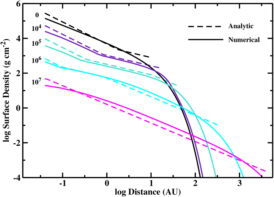
Figure 1: Time evolution of the surface density of a gaseous disk ($M_{d,0}$ = 0.04 $\rm M_{\odot}$, $R_{d,0}$ = 10 AU, $\alpha$ = $10^{-2}$) surrounding a 1 $\rm M_{\odot}$ star. Dashed lines show results for the analytic disk model of Chambers (2009); solid lines show results for our numerical solution of the diffusion equation. Despite small differences in the initial conditions, the numerical solution tracks the analytic model.

Figure 1 compares analytic and numerical results for a disk with $\alpha=10^{-2}$, $M_{d,0}$ = 0.04 $\rm M_{\odot}$, and $R_{0}$ = 10 AU surrounding a star with $M_{\star}$ = 1 $\rm M_{\odot}$. The numerical solution tracks the analytic model well. At early times, the surface density declines steeply in the inner disk (where dust grains evaporate) and more slowly in the outer disk (where viscous transport dominates). At late times, irradiation dominates the energy budget; the surface density then falls more steeply with radius.

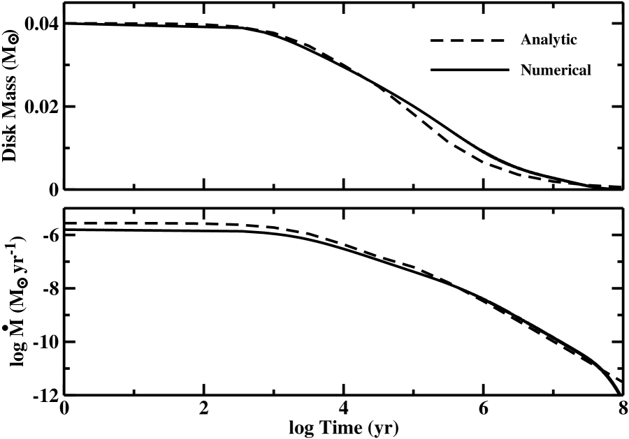
Figure 2: Time evolution of the disk mass (upper panel) and disk accretion rate onto the central star (lower panel) for the analytic and numerical solutions in Figure 1.

Figure 2 compares the evolution of the disk mass and accretion rate at the inner edge of the disk. In both solutions, the disk mass declines by a factor of roughly two in 0.1 Myr, a factor of roughly four in 1 Myr, and a factor of roughly ten in 10 Myr. Over the same period, the mass accretion rate onto the central star declines by roughly four orders of magnitude.

In addition to viscous evolution, we consider photoevaporation of disk material. Following Alexander & Armitage (2007), we assume high energy photons from the central star ionize the disk and drive a wind. As long as the inner disk is optically thick, recombination powers a ‘diffuse wind,’ where the change in surface density is

$$(\frac{\partial\Sigma}{\partial t})_{diffuse}=-2n_{0}(R)u_{0}(R)\mu m_{H}~{}.$$ (13)

In this expression,

$$n_{0}(R)=0.14\left(\frac{3\Phi_{\star}}{4\pi\alpha_{B}R_{g}^{3}}\right)^{1/2}\left(\frac{2}{(R/R_{g})^{15/2}+(R/R_{g})^{25/2}}\right)^{1/5}~{},$$ (14)

and

$$u_{0}(R)=0.3423~{}c_{s,w}~{}\left(\frac{R}{R_{g}}-0.1\right)^{0.2457}~{}e^{-0.3612~{}(R/R_{g}-0.1)}~{}.$$ (15)

The recombination coefficient is $\alpha_{B}=2.58\times 10^{-13}$ cm³ s^-1 (Cox, 2000). The gravitational radius is $R_{g}=GM_{\star}/c_{s,w}^{2}$, where $c_{s,w}$ = 10 $\rm km~{}s^{-1}$ is the sound speed in the wind. For typical stars, the luminosity of H-ionizing photons, $\Phi_{\star}$, is $\sim$ $10^{40}$–$10^{42}$ s^-1. However, Owen et al. (2010) show that X-rays drive a more powerful wind than lower energy photons. Here, we assume that the mass loss rate in the wind, $\dot{M}_{wind}=\int 2\pi R~{}\partial\Sigma/\partial t~{}dR$, is a free parameter and consider disk evolution for a range in $\dot{M}_{wind}$. This approach is equivalent to assuming a range in $\Phi_{\star}$.

As the disk evolves, the diffuse wind removes more and more material throughout the disk. Eventually, the inner disk becomes optically thin to ionizing photons. Ionization then drives a ‘direct wind.’ The change in surface density with time is then much larger,

$$(\frac{\partial\Sigma}{\partial t})_{direct}=0.47~{}\mu~{}m_{H}~{}c_{s,w}\left(\frac{\Phi_{\star}}{4\pi\alpha_{B}(H/R)R_{in}^{3}(t)}\right)^{1/2}\left(\frac{R}{R_{in}(t)}\right)^{-2.42}~{}~{},~{}~{}R>R_{in},$$ (16)

where $R_{in}(t)$ is the inner edge of the optically thick portion of the disk. Inside $R_{in}(t)$, the mass loss rate from the disk is zero.

For mass loss rates $\dot{M}_{wind}\approx 10^{-10}-10^{-8}$ $\rm M_{\odot}~{}yr^{-1}$, the surface density evolution of a viscous disk with photoevaporation follows the evolution in Figure 1 for $\sim 10^{5}-10^{6}$ yr. As the accretion rate through the disk drops, mass loss from the wind becomes more and more important. Once the inner disk becomes optically thin, the direct wind rapidly empties the inner disk of material. As the system evolves, the size of this inner ‘hole’ grows from $R_{h}\approx R_{g}\approx$ 3 AU to $R_{h}\approx$ 30–100 AU in 0.01–0.1 Myr (see also Alexander & Armitage, 2009; Owen et al., 2010). A few thousand years later, the gaseous disk is gone.

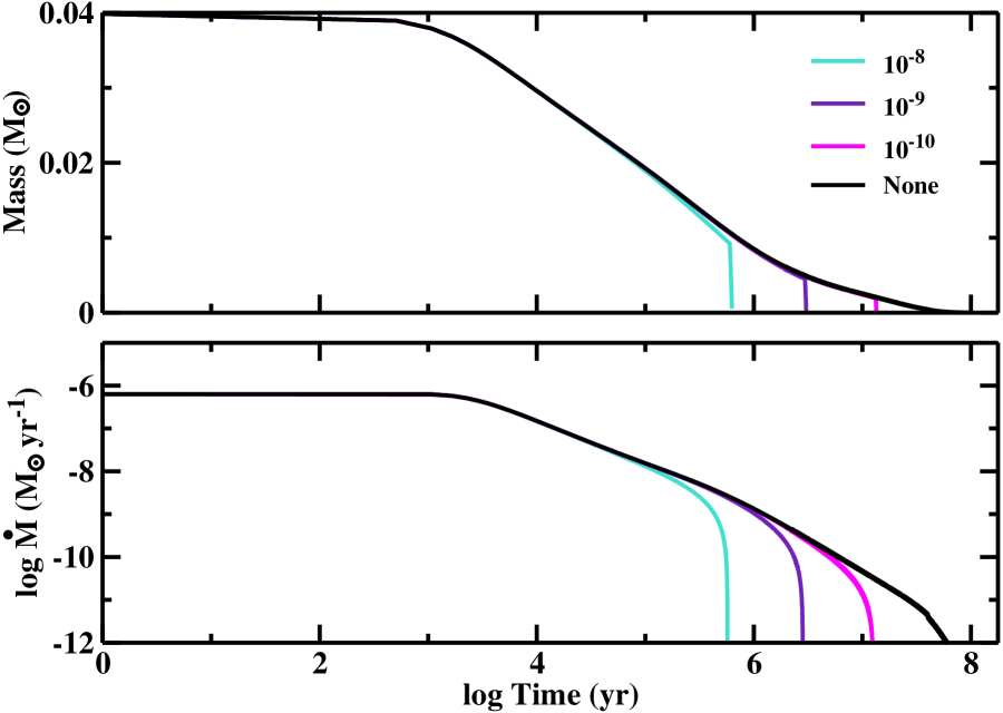
Figure 3: As in Figure 2 for disks with photoevaporative winds. The legend in the upper panel indicates the mass loss rate of the wind in units of $\rm M_{\odot}~{}yr^{-1}$.

Figure 3 shows the variation of disk mass and mass accretion rate for the disk in Figure 2 and several mass loss rates. In general, the wind starts to empty the disk when the mass accretion rate through the disk falls below the mass loss rate in the wind (see Alexander & Armitage, 2009; Owen et al., 2010, and references therein). For very low mass loss rates, $\dot{M}_{wind}=10^{-10}$ $\rm M_{\odot}~{}yr^{-1}$, the wind evaporates the disk on timescales of 10 Myr (see also Alexander & Armitage, 2007, 2009). As the mass loss rate from photoevaporation grows, the disk evaporates on shorter and shorter timescales. For $\dot{M}_{wind}=10^{-8}$ $\rm M_{\odot}~{}yr^{-1}$, the disk disappears on timescales shorter than 1 Myr.

These evolutionary models capture the main observable features of disks around pre-main sequence stars with ages of 1–10 Myr. For 1 Myr-old young stars, disk masses of $\sim$ 0.001–0.1 $\rm M_{\odot}$ and mass accretion rates of $1-100\times 10^{-10}$ $\rm M_{\odot}~{}yr^{-1}$ are common (Gullbring et al., 1998; Hartmann et al., 1998; Andrews & Williams, 2005, 2007). Typical disk lifetimes are 1–3 Myr (Hartmann et al., 1998; Haisch, Lada, & Lada, 2001). Few pre-main sequence stars have ages larger than $\sim$ 10 Myr (Currie et al., 2007; Mamajek, 2009; Kennedy & Kenyon, 2009). Thus, these calculations yield reasonable physical conditions for planet formation.

In our previous calculations, we set the surface density of the gaseous disk as $\Sigma=\Sigma_{0}x_{m}a^{-n}e^{-t/t_{g}}$, with $x_{m}$ as a scaling factor, $n$ as a constant power law, and $t_{g}$ as a constant gas depletion time. In our new approach, adopting an analytic (Chambers, 2009) or a numerical (eq. 1) solution to the radial diffusion equation has several important advantages for little computational effort.

• Following the evolution of the mass accretion rate onto the central star enables robust comparisons between observations of accretion in pre-main sequence stars with the timing of planet formation throughout the disk.

• Treating the evolution of photoevaporation allows us to make links between the so-called transition disks and the formation of planets (e.g., Alexander & Armitage, 2009).

• Tracking the time evolution of the radial position of the snow line (e.g., Kennedy & Kenyon, 2008) in a physically self-consistent fashion gives us a way to include changes in the composition of planetesimals with time.

• Calculating the radial expansion of the disk with time provides a way to compare the observed properties of protostellar disks (e.g., Andrews & Williams, 2005, 2007, 2009) with the derived properties of planet-forming disks.

It is straightforward to derive the properties of power-law disks that yield results similar to those of our new calculations. In analytic and numerical solutions to the diffusion equation, the viscous time $t_{\nu}\approx R^{2}/3\nu$ is roughly the gas depletion time $t_{g}$. For the Chambers (2009) analytic approach, $t_{\nu}\approx$ 4 Myr $(\alpha/10^{-3})$; for our numerical solution, $t_{\nu}\approx$ 1 Myr $(\alpha/10^{-3})$. In previous calculations, we adopt $t_{g}$ = 10 Myr; thus, new calculations with $\alpha=1-4\times 10^{-4}$ roughly correspond to the disks in Kenyon & Bromley (2008, 2009, 2010).

The new calculations generally yield shallower power law slopes – $n$ = 0.6 for Chambers (2009) and $n$ = 1 for our numerical solution – than the $n$ = 1.0–1.5 assumed in our previous studies. Because the timescale for planet formation is $t\propto a^{n+1.5}$ (see Kenyon & Bromley, 2008, and references therein), planets form relatively faster in the outer disk in these new calculations. However, the range of disk masses considered here, $M_{d,0}$ = 0.01–0.1 $\rm M_{\odot}$, overlaps the $M_{d,0}$ = 0.0003–0.25 $\rm M_{\odot}$ adopted in Kenyon & Bromley (2010). Thus, calculations with similar initial disk masses and similar initial size distributions of planetesimals will yield similar timescales for the formation of the first oligarchs.

As a concrete example, we compare several disk surface density distributions quantitatively. In Kenyon & Bromley (2008, 2009, 2010), we often adopted an initial surface density distribution of solid material, $\Sigma$ = 30 g cm^-2 $x_{m}$ (a / 1 AU)^-3/2. At 5 AU, our numerical solutions for disks with $M_{d,0}$ = 0.1 $\rm M_{\odot}$ and $R_{d,0}$ = 30 AU have the same surface density as power law disks with $x_{m}$ = 3. For the same initial disk mass and radius, the Chambers (2009) analytic model has the same surface density as power law disks with $x_{m}\approx$ 2.5. For identical initial conditions and equivalent viscous timescales, these three surface density distributions yield similar evolutionary times for the growth of protoplanets.

2.2 Coagulation Code

Kenyon & Bromley (2008) describe the main details of the coagulation code we use to calculate the growth of small solid particles (planetesimals) into planets. Briefly, we perform calculations on a cylindrical grid with inner radius $R_{in}$ and outer radius $R_{out}$. The model grid contains $N$ concentric annuli with widths $\delta R_{i}$ centered at radii $R_{i}$. Calculations begin with a mass distribution $n(m_{ik}$) of planetesimals with horizontal and vertical velocities $h_{ik}(t)$ and $v_{ik}(t)$ relative to a circular orbit. The horizontal velocity is related to the orbital eccentricity, $e_{ik}^{2}(t)$ = 1.6 $(h_{ik}(t)/V_{K,i})^{2}$, where $V_{K,i}$ is the circular orbital velocity in annulus $i$. The orbital inclination depends on the vertical velocity, $i_{ik}^{2}(t)$ = sin${}^{-1}(2(v_{ik}(t)/V_{K,i})^{2})$.

The mass and velocity distributions of planetesimals evolve in time due to inelastic collisions, drag forces, and gravitational forces. The collision rate is $n\sigma vf_{g}$, where $n$ is the number density of objects, $\sigma$ is the geometric cross-section, $v$ is the relative velocity, and $f_{g}$ is the gravitational focusing factor (Safronov, 1969; Lissauer, 1987; Spaute et al., 1991; Wetherill & Stewart, 1993; Weidenschilling et al., 1997; Kenyon & Luu, 1998; Krivov et al., 2006; Thébault & Augereau, 2007; Löhne et al., 2008; Kenyon & Bromley, 2008). The collision outcome depends on the ratio of the collision energy needed to eject half the mass of a pair of colliding planetesimals $Q_{d}^{\star}$ to the center of mass collision energy $Q_{c}$. If $m_{1}$ and $m_{2}$ are the masses of two colliding planetesimals, the mass of the merged planetesimal is

$$m=m_{1}+m_{2}-m_{ej}~{},$$ (17)

where the mass of debris ejected in a collision is

$$m_{ej}=0.5~{}(m_{1}+m_{2})\left(\frac{Q_{c}}{Q_{d}^{*}}\right)^{9/8}~{}.$$ (18)

This approach allows us to derive ejected masses for catastrophic collisions with $Q_{c}\sim Q_{d}^{*}$ and for cratering collisions with $Q_{c}\ll Q_{d}^{*}$ (see also Wetherill & Stewart, 1993; Williams & Wetherill, 1994; Tanaka et al., 1996; Stern & Colwell, 1997; Kenyon & Luu, 1999; O’Brien & Greenberg, 2003; Kobayashi & Tanaka, 2010). Consistent with numerical simulations of collision outcomes (e.g., Benz & Asphaug, 1999; Leinhardt et al., 2008; Leinhardt & Stewart, 2009), we set

$$Q_{d}^{*}=Q_{b}r^{\beta_{b}}+Q_{g}\rho_{g}r^{\beta_{g}}$$ (19)

where $Q_{b}r^{\beta_{b}}$ is the bulk component of the binding energy, $Q_{g}\rho_{g}r^{\beta_{g}}$ is the gravity component of the binding energy, $r$ is the radius of a planetesimal, and $\rho_{g}$ is the mass density of a planetesimal.

To compute the evolution of the velocity distribution, we include collisional damping from inelastic collisions and gravitational interactions. For inelastic and elastic collisions, we adopt the statistical, Fokker-Planck approaches of Ohtsuki (1992) and Ohtsuki, Stewart, & Ida (2002), which treat pairwise interactions (e.g., dynamical friction and viscous stirring) between all objects in all annuli (see also Stewart & Ida, 2000). As in Kenyon & Bromley (2001), we add terms to treat the probability that objects in annulus $i$ interact with objects in annulus $j$ (see also Kenyon & Bromley, 2004b, 2008).

2.2.1 Small particles

In most of our previous calculations, we calculate the evolution of particles with radii larger than the ‘stopping radius,’ $r_{s}\approx$ 0.5–2 m at 5–10 AU (Adachi et al., 1976; Weidenschilling, 1977; Rafikov, 2004). Although they are subject to gas drag, these particles are not well-coupled to the gas. Here, we also consider the evolution of smaller particles entrained by the gas (see also Kenyon & Bromley, 2009). Following Youdin & Lithwick (2007), we derive the Stokes number

$$St=\frac{r\rho_{g}\Omega}{\rho c_{s}}~{},$$ (20)

where $\rho=\Sigma/2H$ is the gas density. The vertical scale height of small particles is then

$$H_{s}=\left\{\begin{array}[]{cll}H~{},&&St\leq\alpha\\ \sqrt{\frac{\alpha}{St}}~{}H~{},&&St>\alpha\\ \end{array}\right.$$ (21)

We assume that entrained small particles have vertical velocity $v=H_{s}\Omega$ and horizontal velocity $h=1.6v$.

Estimating accretion rates of small particles by embedded protoplanets is a challenging problem. For particles with $St\sim 1$, accretion rates depend on the strength of the planet’s gravity relative to forces that couple particles to the gas. Recently, Ormel & Klahr (2010) began to address this issue with an analysis of interactions between protoplanets and particles (loosely) coupled to the gas. After identifying three classes of encounters, they derive growth rates as a function of $m$, $St$, and the local properties of the gas. For massive protoplanets with $r\gtrsim$ 1000 km, they derive short growth times, $\sim 10^{3}$ yr, for particles with $10^{-1}<St<10$.

Here, we adopt a simple prescription for accretion of small particles with $St\lesssim$ 1. Small protoplanets with $r<100$ km do not have strong enough gravitational fields to wrest small particles from the gas. Thus, we assume small protoplanets cannot accrete particles with $St<1$. The Ormel & Klahr (2010) results suggest large protoplanets accrete particles with $St<10^{-3}$ on long timescales, $\gtrsim$ 1 Myr. Thus, we also assume protoplanets of any size cannot accrete these particles. For particles with $St>10^{-3}$, we assume accretion proceeds as in our standard formalism with collision rates $n\sigma vf_{g}$, where the cross-section $\sigma$ includes the enhanced radius of the protoplanet discussed in §2.2.2. Our approach generally yields growth rates a factor of 1–10 smaller than those of Ormel & Klahr (2010). Thus, our formation times are longer than timescales derived from a more rigorous approach. For the calculations in this paper, however, this accuracy is sufficient to explore the impact of disk mass and viscosity on the formation of gas giant planets. In future papers, a more comprehensive treatment of small particle accretion and gas drag will yield a better understanding of the role of the local properties of the gas on planet formation.

Aside from enabling protoplanets to accrete smaller particles at large rates, including small particles with $r\lesssim$ 1 m allows us to derive a more accurate calculation for the time evolution of debris from the collisional cascade. Compared to results in Kenyon & Bromley (2008, 2010), estimates for the abundance of very small grains with $r\sim$ 1–10 $\mu$m now rely on extrapolation over 3 orders of magnitude in radius instead of 6. Thus, this addition yields more accurate predictions for the variation of grain emission as a function of time (see, for example, Kenyon & Bromley, 2008, 2010).

2.2.2 Planetary atmospheres

As planets grow, they acquire gaseous atmospheres. Initially, the radius of the atmosphere $R_{a}$ is well-approximated by the smaller of the Bondi radius $R_{B}$ and the Hill radius $R_{H}$:

$$R_{a}=\left\{\begin{array}[]{cll}R_{B}=\frac{GM_{p}}{c_{s}^{2}}~{},&&R_{B}<R_{H}\\ R_{H}=\left(\frac{M_{p}}{3M_{\star}}\right)^{1/3}a~{},&&R_{B}>R_{H}\\ \end{array}\right.$$ (22)

where $M_{p}$ is the mass of the planet and $a$ is the semimajor axis of the planet’s orbit around the central star. For low mass planets, $R_{H}>R_{B}$. Requiring $R_{B}>R_{P}$, where $R_{P}$ is the radius of the planet, an icy planet with a mass density of 1 g cm^-3 starts to form an atmosphere when $M_{p}\gtrsim 3\times 10^{25}$ g.

Once planets develop a small atmosphere, they accrete small particles more rapidly (Podolak et al., 1988; Kary et al., 1993; Inaba & Ikoma, 2003; Tanigawa & Ohtsuki, 2010). As small particles approach the planet, atmospheric drag reduces their velocities. Smaller velocities increase gravitational focusing factors, enabling very rapid accretion (see also Chambers, 2008; Rafikov, 2010). Because the extent of the atmosphere depends on the accretion luminosity, calculations need to find the right balance between the extent of the atmosphere and the accretion rate (and luminosity). Here, we follow Inaba & Ikoma (2003) and solve for the structure of an atmosphere in hydrostatic equilibrium around each planet with $M_{p}\gtrsim 3\times 10^{25}$ g. For each smaller planetesimal with mass $m$, we calculate the enhanced radius $R_{E}(M_{p},~{}m)$, which replaces the physical radius in our derivation of cross-sections and collision rates.

This approach shortens growth times by factors of 3–10. In Chambers (2006), protoplanets with atmospheres grow 3–4 times faster at 5 AU than protoplanets without atmospheres (see also Inaba & Ikoma, 2003). To confirm these results, we repeated the calculations of Kenyon & Bromley (2009) for protoplanets with atmospheres. In a power-law disk with $x_{m}$ = 5, our previous calculations yielded 10 $\rm M_{\oplus}$ protoplanets on timescales of $\sim$ 3 Myr. Repeating these calculations for protoplanets with planetary atmospheres results in growth times shorter by factors of 5–10, $\sim$ 0.3–0.5 Myr. Several numerical tests suggest that different fragmentation laws produce factor of 1.5–2 changes in the growth time for protoplanets with atmospheres (see also Chambers, 2006, 2008). Kenyon & Bromley (2009) derived only 10% to 20% variations in growth times for a similar range in fragmentation laws. Thus, growth times are more sensitive to fragmentation when protoplanets have atmospheres.

2.2.3 Gas accretion

As planets continue to grow, they begin to accrete gas from the disk. Although the minimum mass required to accrete gas varies with the accretion rate of the planet, the properties of the disk near the planet, and the distance of the planet from the central star, a typical minimum mass is $\sim$ 1–10 $\rm M_{\oplus}$ (Mizuno, 1980; Stevenson, 1982; Ikoma et al., 2000; Hori & Ikoma, 2010; Rafikov, 2006, 2010). Once gas accretion begins, the planet mass grows rapidly until it removes most of the gas in its vicinity, either by depleting the disk entirely or by opening up a gap between the planet and the rest of the disk. The planet then grows more slowly and may start to migrate through the disk (e.g., Lin & Papaloizou, 1986; Lin et al., 1996; Ward, 1997; D’Angelo et al., 2010).

Here, we approximate the complicated physics of gas accretion and the evolution of the atmosphere with a simple formula (see also Veras & Armitage, 2004; Ida & Lin, 2005; Alexander & Armitage, 2009). The growth rates reviewed in D’Angelo et al. (2010) suggest

$$\dot{M}_{g}\approx\dot{M}_{0}\frac{M_{p}}{M_{0}}~{}\frac{\Sigma\Omega^{2}}{c_{s}}~{}e^{-((\mu-\mu_{0})/\sigma_{m})^{2}}~{},$$ (23)

where $\dot{M}_{0}$ is a typical maximum accretion rate, $M_{0}\approx$ 0.1 $\rm M_{J}$ (1 $\rm M_{J}$ is the mass of Jupiter), $\mu$ = log $M_{p}$, $\mu_{0}$ = log $M_{0}$, and $\sigma_{m}\approx$ 2/3. This functional form captures the rapid increase in the accretion rate from the minimum core mass of 1–10 $\rm M_{\oplus}$ to larger core masses, the peak accretion rate at masses of roughly 10% the mass in Jupiter, and the decline in the accretion rate once the planet opens up a gap in the disk. Detailed numerical simulations suggest maximum accretion rates of 1 Jupiter mass every 0.01–0.1 Myr (e.g. Lissauer & Stevenson, 2007; D’Angelo et al., 2010; Machida et al., 2010, and references therein). For simplicity, we consider $\dot{M}_{0}$ a free parameter; we set a rate appropriate for a Jupiter mass gas giant in a disk with $\Sigma$ = 100 g cm^-2, $\Omega=1.78\times 10^{-8}$ s^-1 (5 AU), and $c_{s}$ = 0.67 $\rm km~{}s^{-1}$ and use equation (23) to scale this rate throughout the disk.

To remove accreted gas from the disk in our numerical simulations of disk evolution, we set the change in surface density as

$$(\frac{\partial\Sigma}{\partial t})_{gas}=-\frac{\dot{M}_{g}}{2\pi R\Delta R}~{},$$ (24)

where $R$ is the semimajor axis of the planet and $\Delta R$ is the width of the annulus. Combined with photoevaporation from the central star, this expression yields

$$(\frac{\partial\Sigma}{\partial t})_{ext}=\left\{\begin{array}[]{cll}(\frac{\partial\Sigma}{\partial t})_{diffuse}+(\frac{\partial\Sigma}{\partial t})_{gas}~{},&&R_{in}\approx R_{\star}\\ (\frac{\partial\Sigma}{\partial t})_{direct}+(\frac{\partial\Sigma}{\partial t})_{gas}~{},&&R_{in}\gg R_{\star}\\ \end{array}\right.$$ (25)

where $R_{in}$ is the inner edge of the optically thick portion of the disk.

Although we use equation (23) to derive gas accretion rates for the analytic disk model, we do not remove the accreted mass from the disk. To place some limit on the amount of mass accreted by gas giants, we halt gas accretion when the total mass in gas giants exceeds the total remaining mass in the disk.

2.2.4 Evolution of R and L of planets

Throughout this phase, the radius of the planet $R_{p}$ depends on the accretion rate and the properties of the atmosphere (e.g., Hartmann et al., 1997; Papaloizou & Nelson, 2005; Chabrier et al., 2007; Lissauer & Stevenson, 2007; Baraffe et al., 2009; D’Angelo et al., 2010). Before the planet opens a gap in the disk, accretion is roughly spherical; after the gap forms, the planet accretes material from a thin disk-like structure within the planet’s Hill sphere (e.g., Nelson et al., 2000; D’Angelo & Lubow, 2008). For planets with masses much larger than Neptune, disk accretion provides most of the gas. Thus, to derive a simple estimate for the evolution of $R_{p}$, we solve the energy equation for a polytrope of index $n=1.5$ accreting material from a gaseous disk (e.g. Hartmann et al., 1997):

$$\frac{\dot{R_{p}}}{R_{p}}=\left(\frac{7}{3}~{}\eta-\frac{1}{3}\right)\frac{\dot{M_{p}}}{M_{p}}~{}-~{}\frac{7}{3}\left(\frac{L}{GM_{p}^{2}/R_{p}}\right)~{}.$$ (26)

Here, $L$ is the planet’s photospheric luminosity in erg s^-1; $1-\eta$, where $\eta\leq 1$, measures the fraction of the accretion energy radiated away before material hits the planet’s photosphere.

Solving equation (26) requires a relation for $L$. When $\dot{M}$ = 0, planets resemble $n$ = 0.5–1 polytropes, with $R_{p}\propto M_{p}^{m}$ and $-1/8\leq m\leq 1/10$ (e.g., Saumon et al., 1996; Fortney et al., 2009). For this phase, we derive a simple expression from published evolutionary tracks (e.g., Burrows et al., 1997; Spiegel et al., 2010; Baraffe et al., 2003, 2008):

$$L\approx 10^{-9}~{}{\rm L_{\odot}}~{}\left(\frac{M_{p}}{1~{}M_{J}}\right)^{0.25}~{}\left(\frac{R_{p}}{1~{}R_{J}}\right)^{15},~{}$$ (27)

where $R_{J}$ is the radius of Jupiter. Accretion energy tends to expand planets considerably (e.g., Pollack et al., 1996; Marley et al., 2007; D’Angelo et al., 2010). To treat this phase, we derive a simple expression from published model atmosphere calculations applied to an $n=1.5$ polytrope (Saumon et al., 1996; Fortney et al., 2009, and references therein):

$$L\approx 10^{-6}~{}{\rm L_{\odot}}~{}\left(\frac{M_{p}}{1~{}M_{J}}\right)~{}\left(\frac{R_{p}}{1~{}R_{J}}\right)^{3}.~{}$$ (28)

When the planet has a radius $R_{t}\approx 1.78(M_{p}/1~{}M_{J})^{0.06}R_{J}$, these relations yield the same luminosity. Thus, we use equation (27) for $R(M_{p})>R_{t}$ and $\dot{M}_{g}>$ 0 and equation (28) otherwise.

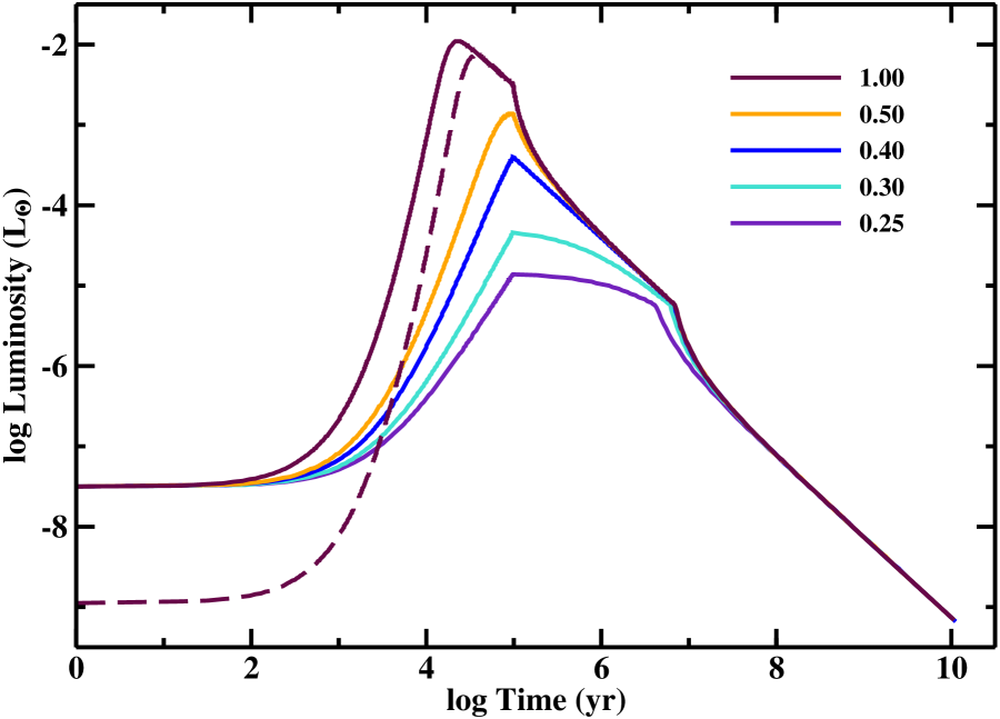
Figure 4: Luminosity evolution for a gas giant planet using the prescription in equations (26)–(28). Starting with an initial mass of 10 $\rm M_{\oplus}$ and an initial radius of 1 $\rm R_{J}$, the planet accretes gas at a rate of $10^{-5}$ $\rm M_{J}$ yr^-1 until it reaches a mass of 1 $\rm M_{J}$. Solid curves show the evolution for various $\eta$. When $\eta$ is small; the planet accretes cold material and has a small peak luminosity. When $\eta$ is large, the planet accretes hotter material, expands, and has a large peak luminosity. At late times, all curves converge on a single evolutionary track which yields a Jupiter-radius planet at 4–6 Gyr. The dashed curve illustrates how the evolution changes for planets with initial radii of 0.33 $\rm R_{J}$ (comparable to the radius of Neptune).

Despite its simplicity, this approach yields reasonable results for $L(t)$ and $R_{p}(t)$. In the example of Fig. 4–5, the calculation starts with a 10 $\rm M_{\oplus}$, 1 $\rm R_{J}$ planet accreting at a rate of $10^{-5}$ $\rm M_{J}~{}yr^{-1}$ until it reaches a mass of 1 $\rm M_{J}$. Before the planet reaches its final mass, the luminosity increases exponentially with time. Once accretion stops, the luminosity declines. Peak luminosity and radius depend on $\eta$; planets that accrete hotter material (larger $\eta$) expand more than planets that accrete colder material (smaller $\eta$). For $\eta\approx$ 0.3–0.4, our peak luminosities of $\sim 10^{-4}$ $\rm L_{\odot}$ are similar to those of more detailed calculations (Pollack et al., 1996; Marley et al., 2007; D’Angelo et al., 2010). At late times, evolution for all $\eta$ converges on a single track for $L(t)$ and $R_{p}(t)$. This track yields a radius of 1.03 $\rm R_{J}$ at 4.5 Gyr.

Although this approach is not precise, it serves our purposes. The model yields planetary radii with sufficient accuracy ($\pm$ 10%) to derive the merger rate of growing planets from dynamical calculations with our $N$-body code. The estimated luminosity is also accurate enough to serve as a reasonable starting point for more detailed evolutionary calculations, as in Burrows et al. (1997) or Baraffe et al. (2003). This formalism is also flexible: it is simple to adopt better prescriptions for the luminosity or an energy equation with a different polytropic index.

2.3 $N$-body Code

Bromley & Kenyon (2006) provide a description of the $N$-body component of our hybrid code. To solve the equations of motion for a set of interacting particles, we use an adaptive algorithm with sixth-order time steps, based either on Richardson extrapolation (Bromley & Kenyon, 2006) or a symplectic method (Yoshida, 1990; Kinoshita, Yoshida, & Nakai, 1991; Wisdom & Holman, 1991; Saha & Tremaine, 1992). The code calculates gravitational forces by direct summation and evolves particles accordingly. In our earlier version, we performed integrations in terms of phase-space variables defined relative to individual Keplerian frames, following the work of Encke (Encke, 1852; Vasilev, 1982; Wisdom & Holman, 1991; Ida & Makino, 1992; Fukushima, 1996; Shefer, 2002); our latest version can track center-of-mass frame coordinates instead. This feature may be useful in instances where stellar recoil is important. As before, the code evolves close encounters – including mergers – between pairs by solution of Kepler’s equations in the pairs’ center of mass frame. The algorithm also includes changes in eccentricity, inclination, and semimajor axis, derived from the Fokker-Planck and gas drag algorithms in the coagulation code.

The 2006 version and the new version of $N$-body code can track the force from a dusty or gaseous disk. The older code handles only toy models for the gaseous disk, consisting of a power law surface density profile and an exponential decay in time. The new code includes the more realistic disk potential derived in §2.1. The code represents a disk in annular bins with time-varying surface density specified by the physical model. Although the current code does not treat the lack of gravitational force from gaps in the disk produced by gas giant planets, this extra force is small compared to the forces from the rest of the disk and gas giant planets. Once this feature is included, we can then self-consistently track the dynamics of gas giants in an evolving gaseous disk.

Appendix A provides some background and details of our method to treat the gravity of the gaseous disk. To summarize, we approximate the disk as axisymmetric with a scale height $H$, which is small compared to the orbital distance ($H/a\mathrel{\hbox{\raise 2.15277pt\hbox{$<$}\hbox to0.0pt{\hss\lower 2.15277pt\hbox{$\sim$}}}}0.1$). The acceleration that the disk produces on a planet near the disk midplane is then fast to calculate. When the disk has a power-law surface density, a simple analytical expression suffices. If the disk has more complicated radial structure (§2.1), then we split it up into constant-density annuli and calculate the contribution of each annulus to the acceleration at some point near the disk midplane. We repeat this calculation for a set of $O(10^{4})$ radial points at the beginning of a simulation, and interpolate with a cubic spline thereafter to find the disk acceleration at the location of the $N$ objects. As the surface density of the disk evolves, the code updates the date for the spline fit.

In addition to gas, the new version of the $N$-body code includes the gravity of non-physical objects representing dust or planetesimals. As in the SyMBA code of Duncan, Levison, & Lee (1998), we use massless “tracer” particles, which simply respond to the gravitational potential produced by the central star and planets. We use the evolution of the tracers to inform the coagulation code of the $de/dt$, $di/dt$, and $da/dt$ induced by massive planets in the $N$-body code. We also have a second population of massive “swarm” particles, which have mutual interactions with planets but do not interact with either tracers or with each other. The swarm thus consists of super-particles which represent the ensemble of small objects that interact with each other statistically in the coagulation code and which also interact dynamically with planets in the $N$-body code. Independently of the tracers, we can use the swarm particles to inform the coagulation code of the $de/dt$, $di/dt$, and $da/dt$ induced by massive planets in the $N$-body code. More importantly, we use the mutual interactions of swarm and $N$-body particles to calculate the response of planets to the surface density and velocity distributions of the swarm. In addition to the tests in §3, Bromley & Kenyon (2011) describe some applications of the interaction between swarm and $N$-body particles.

In terms of comparative computational cost, planets are expensive, tracers are cheap, and swarm particles are in between. Even without mutual interactions, the swarm particles can be a considerable burden in long-term integrations. To lighten this computational load, we evolve the star and planets independently of the swarm during a single coarse-grain timestep, allowing the code to take as many substeps as necessary. Then, we interpolate the resulting planet trajectories to calculate the gravitational forces needed to update the swarm. When we use massive swarm particles, we allow the planets to deviate from their interpolated path in response to the smaller objects. This approach is valid only when the net forces on the planets from the swarm vary slowly in time, and when the our simple third-order interpolation of the planet’s trajectory over a coarse timestep is realistic. With this approach, there is a risk of lower accuracy for the very rare events when some members of the swarm interact with a pair of closely-interacting $N$-body particles. Our 3rd-order interpolation then does not yield a robust representation of the trajectories of these swarm particles. Detailed tests show that reduced accuracy only occurs for the very few swarm particles within 1–2 Hill radii of the pair of $N$-bodies, has a negligible impact on the trajectory of the $N$-body particles, and does not influence the outcome (merger or scattering event) of the interaction between the two $N$-bodies.

2.4 $N$-body code tests

We put the new version of the $N$-body code through the same diagnostics as in Bromley & Kenyon (2006). To assess accuracy and dynamic range, we perform long-term orbit integrations of the major planets, as well as integrations of the planets with their masses scaled by a factor of fifty (Duncan, Levison, & Lee, 1998; Bromley & Kenyon, 2006). We also track the motion of tight binaries in orbit around a central star. In one limit, we evolve a close pair of Jupiter-mass objects (Duncan, Levison, & Lee, 1998); in another, we simulate a surface-skimming satellite above the Earth as it orbits the Sun. We also set up pairs of planets on closely-spaced circular orbits and evolve them to see whether we can resolve the critical separation that determines whether their orbits cross (Gladman, 1993). With these tests we verify that the new code can replicate the results illustrated in Figures 1–4 of Bromley & Kenyon (2006).

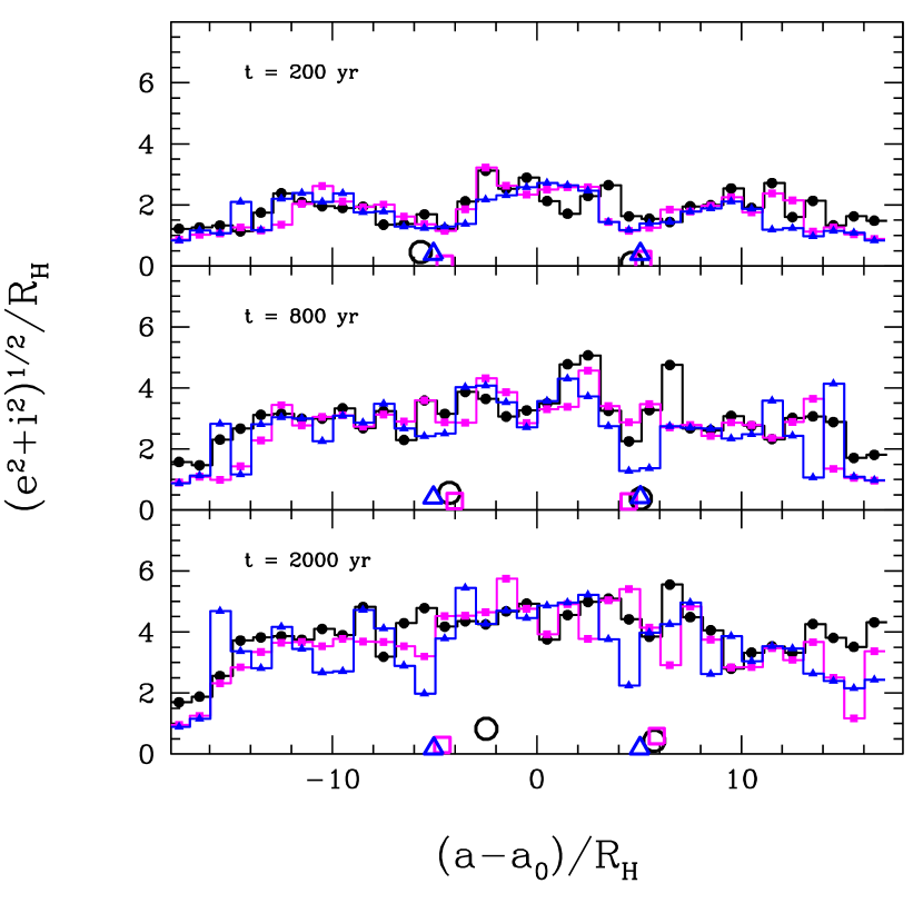
Figure 6: The evolution of $(e^{2}+i^{2})^{1/2}$ (in units of Hill radii) of a particle disk with two embedded planets, as in Kokubo & Ida (1995). The abscissa gives the relative orbital separation in terms of the difference between the semimajor axis $a$ and a reference radius $a_{0}=1$ AU. The histograms correspond to the disk particles; the symbols represent the two planets. The colors and symbol styles distinguish simulations: black histograms and circles indicate fully interacting massive particles, blue lines and triangles show data from a massive disk of swarm particles with no self-gravity, while magenta histograms and squares correspond to a massless disk composed of tracers.

To save computation time, the new code evolves tracers and swarm particles with lower temporal resolution than with the planets. To verify that the resulting orbits are reasonable, we follow Kokubo & Ida (1995) in simulating gravitational stirring of a planetesimal swarm by a pair of planets. Two $2\times 10^{26}$ g planets are separated by 10 $R_{H}$ and are embedded in the middle of an annulus of 800 $2\times 10^{24}$ g objects, which is 35 $R_{H}$ wide and centered at a distance of 1 AU from a 1 $\rm M_{\odot}$ star. All objects are initially on circular orbits. We evolve this system treating all particles as mutually interacting massive bodies, then with the disk composed of massive swarm particles that interact with the planets only, and finally with a massless tracer disk. Figure 6 shows that all three methods yield output that is in good qualitative agreement with previous calculations (Kokubo & Ida, 1995; Weidenschilling et al., 1997; Kenyon & Bromley, 2001; Bromley & Kenyon, 2006).

The final set of tests for the $N$-body code concerns its ability to identify mergers, in particular between planets and swarm particles or tracers. We first confirm that minor changes to the code maintain its accuracy in high-speed mergers between small massive objects (the “grapefruit test” in Bromley & Kenyon, 2006). We then test mergers between planets and tracers or swarm particles explicitly with the more sophisticated method proposed by Greenzweig & Lissauer (1990). We set up (i) a $10^{-6}$ $\rm M_{\odot}$ planet on a circular orbit at 1 AU and (ii) test particles on orbits with eccentricity $e=0.007$, inclination $i=0.2$ degrees, and semimajor axes distributed in two rings (0.977 AU to 0.991 AU and 1.009 AU to 1.023 AU). We evolve the system through a single close encounter between the planet and each test particle to measure the fraction of test particles accreted by the planet. With the planet’s physical radius set to 5300 km, we derive a merger fraction of $0.008\pm 0.001$, consistent with previous estimates (Greenzweig & Lissauer, 1990; Duncan, Levison, & Lee, 1998; Bromley & Kenyon, 2006).

3 MIGRATION

Interactions between a gaseous or planetesimal disk and planets can lead to signification migration, with rates of change in semimajor axis, $da/dt$, that are important on planet formation timescales (Lin & Papaloizou, 1979; Goldreich & Tremaine, 1980; Lin & Papaloizou, 1986; Ward, 1997; Veras & Armitage, 2004; Levison et al., 2007). Migration occurs when a planet perturbs a disk gravitationally. The resulting angular momentum exchange between the planet and the perturbed disk causes the planet to move radially inward or outward. Several types of migration (Ward, 1997) depend on disk and planet properties. When an embedded planet produces a modest perturbation in a massive disk (type I migration), the planet responds to torques from the disk and migrates inwards. When a planet is massive enough to open a radial gap in the disk (type II migration), the planet becomes locked into the global viscous flow and migrates inwards. Type III migration (e.g., Papaloizou et al., 2007) is a fast migration mode associated with smaller planets that efficiently exchange angular momentum with co-orbiting material. As with migration in a planetesimal disk (see Fig. 10), this mode can produce inward or outward migration.

Our code treats all types of migration through the gaseous disk using semianalytical approximations (e.g., Papaloizou et al., 2007). Although we do not include any detailed disk hydrodynamics, the code can smoothly change the semimajor axis and other orbital elements of each planet at any specfied rate.

The code includes another migration mechanism, perhaps “Type 0,” that involves interaction between a massive disk and planets. In an axisymmetric disk that redistributes mass, planets migrate as the disk mass changes. For photoevaporation and viscous transport, the disk mass and gravitational potential change slowly compared to the local dynamical time. The angular momentum of the planet is conserved. By treating the disk and the central star as a point mass with mass $M_{eff}$ acting on a planet at semimajor axis $a$, $aM_{eff}$ is conserved. As the disk vanishes, the planet migrates outward. We provide a few more details of Type 0 migration in Appendix B.

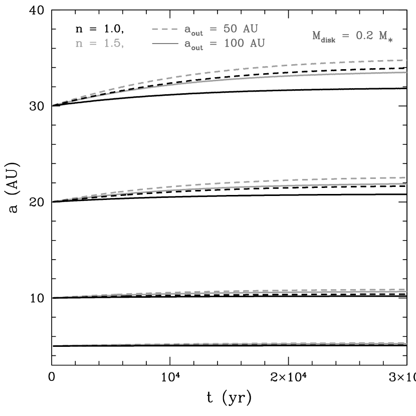
Figure 7: Semimajor axis as a function of time in Type 0 migration. Planets move in response to a decrease in disk mass, for four different massive disks, with surface density $\Sigma\sim a^{-{\rm n}}$, and outer disk radius $a_{out}$ as labeled. The initial mass of each disk is 20% of the stellar mass (1 $\rm M_{\odot}$); the disk mass decays exponentially on a timescale of $10^{4}$ yr. The greatest migration is for the $n=1.5$ disk with an inner edge of 50 AU (gray dashed line), which has the most mass initially concentrated within the orbits of the planets.

Figure 7 illustrates Type 0 migration in a disk with a power law surface density distribution ($\Sigma\propto a^{-n}$) that decays exponentially on a timescale of $10^{4}$ yr. Two of the disks have $n=1$; two others have $n=1.5$. Each pair has an inner edge at 0.1 AU and an outer edge at either 50 AU or 100 AU. In all cases, the initial disk mass is 20% of the mass of the 1 $\rm M_{\odot}$ central star. The migration scales approximately with the amount of disk mass inside a planet’s orbit. Therefore the effect is strongest for a steep slope in surface density and smaller outer disk radius. While this type of migration may not be comparatively strong in magnitude, it may help to alter the orbital dynamics in a disk with closely-packed giant planets.

Type 0 migration pushes planets outward if the disk photoevaporates. It may push planets inwards if mass is flowing in toward the star by viscous processes.

3.1 Migration in a planetesimal disk

As protoplanetary disks evolve, planetesimals become important to the large-scale orbital dynamics of the growing planets. Repeated weak interactions with planetesimals can push a planet radially inwards or outwards. Lin & Papaloizou (1979) and Goldreich & Tremaine (1980) first quantified aspects of this effect analytically; since then, others have explored it numerically (e.g., Malhotra, 1993; Ida et al., 2000; Kirsh et al., 2009). Here, we show that our code can perform similar calculations.

Our first illustration of planet migration follows Kirsh et al. (2009). A 2 $\rm M_{\oplus}$ planet is embedded in a disk of planetesimals, each having a mass $1/600^{\rm th}$ of the planet’s mass. The disk extends from 14.5 AU to 35.5 AU and has a surface density $\Sigma=1.2~{}(a/a_{0})^{-1}$ g cm^-2 where $a_{0}$ = 25 AU. Initially, the planet has $e$ = 0; the planetesimals have $e_{rms}=0.001$ and $i_{rms}$ = 0.5 $e_{rms}$, where ’rms’ is root-mean-squared. The planet stirs nearby planetesimals to large $e$ and ejects some planetesimals from the system (Figure 8). As a reaction to the stirring by the planetesimals, the planet migrates from 25 AU at $10^{4}$ yr to 22 AU at $6\times 10^{4}$ yr, leaving excited planetesimals in its wake. Because the planetesimals have finite masses and encounter the planet sporadically, inward migration is not smooth (Figure 9). Our results agree with previous simulations (see Figs. 3 and 4 of Kirsh et al., 2009).

Our second demonstration of migration follows the work of Hahn & Malhotra (1999). Their disk has $\Sigma\propto a^{-1}$ and total mass of 100 $\rm M_{\oplus}$ between 10 AU and 50 AU. The disk is composed of 1000 planetesimals with $e_{rms}=2i_{rms}=0.01$. With the Solar System’s four major planets initially packed between 5 AU and 23 AU, the system evolves dramatically in time. Dynamical interactions between the planets and planetesimals spread the orbits significantly. Jupiter migrates inwards a small amount; the outer planets migrate outwards in semimajor axis. After $\sim$ 30 Myr, Neptune reaches $a\sim 40$ AU. Figure 10 shows the specifics of the migration with our code. The results compare well with Hahn & Malhotra (1999, lower left panel of their Figure 4).

4 FORMATION OF GAS GIANT PLANETS

To illustrate how gas giants form in our approach, we adopt the analytic disk model of Chambers (2009) with $R_{d,0}$ = 30 AU, $M_{d,0}$ = 0.01, 0.02, 0.04, or 0.1 $\rm M_{\odot}$, and $\alpha$ = $10^{-2}$, $10^{-3}$, $10^{-4}$, or $10^{-5}$. We follow the evolution of disk properties ($\Sigma$, $\dot{M}(R)$, $T_{d}$, etc) on a grid extending from 0.2 AU to $10^{4}$ AU. For the coagulation code, we divide the region between 3 AU and 30 AU into 96 concentric annuli, adopt a dust-to-gas ratio of 0.01, and seed these annuli with planetesimals. To set the gas parameters in the coagulation grid, we interpolate physical variables in the grid for the disk evolution code. For the bulk properties of planetesimals, we follow Leinhardt & Stewart (2009) and adopt parameters for weaker objects with $f_{W}$ = {$Q_{b}$ = $2\times 10^{5}$ erg g^-1 cm^0.4, $\beta_{b}=-0.4$, $Q_{g}$ = 0.33 erg g^-2 cm^1.7, $\beta_{g}$ = 1.3} (see Kenyon & Bromley, 2010, and references therein).

In all theories, the mechanism, timing, and size distribution of planetesimal formation is uncertain (e.g., Rice et al., 2006; Garaud, 2007; Kretke & Lin, 2007; Brauer et al., 2008; Cuzzi et al., 2008; Laibe et al., 2008; Birnstiel et al., 2009; Chiang & Youdin, 2010; Youdin, 2010). To explore how the formation of large planetesimals by the streaming instability (see Youdin, 2010, and references therein) might produce gas giants, we consider two extreme possibilities.

1. Each annulus contains a single large ‘seed’ planetesimal, $r\approx$ 1000 km, and a large population of 0.1–10 cm pebbles. The gas entrains small planetesimals. The growth rate of the seeds then depends on the scale height of the gas, which is set by the viscosity parameter $\alpha$. Because disks with smaller $\alpha$ have smaller vertical scale heights, planets should form more efficiently in disks with smaller $\alpha$.

2. Each annulus contains only large planetesimals, $r\approx 1000$ km, with initial $e=10^{-4}$. Aside from migration, the gas does not affect large planetesimals. However, collision rates scale inversely with the radius of planetesimals (e.g., Goldreich, Lithwick, & Sari, 2004; Kenyon & Bromley, 2008). Thus, planets should form less efficiently than in calculations with a few large seeds and a swarm of small pebbles.

For each of these possibilities, the coagulation code treats the evolution of planetesimals with radii of 1 mm to 3600 km. At the start of each calculation, we assign a seed to the random number generator used to assign integral collision rates (e.g., Wetherill & Stewart, 1993; Kenyon & Luu, 1998). In this way, otherwise identical starting conditions can lead to very different collision histories. As long as the gas density is sufficient to entrain particles with $r\gtrsim$ 1 mm, we distribute collision fragments with $r<$ 1 mm into mass bins with $r$ = 1–2 mm. Otherwise, these particles are lost to the grid. When individual coagulation particles reach masses of $m_{pro}\approx 3\times 10^{26}$ g ($r\approx$ 3600 km), the code promotes these objects into the $N$-body code. After the coagulation code initializes $a$, $e$, $i$, and the longitude of periastron, the $N$-body code follows the changing masses and orbital parameters of promoted objects. Although the $N$-body code can treat the evolution of $N$-bodies with any orbital semimajor axis, we assume that objects with $a\gtrsim 10^{4}-10^{5}$ AU are ejected from the system.

In these calculations, we adopt a single set of parameters for gas accretion onto icy cores. Throughout the disk, gas accretion begins when the core mass is 10 $\rm M_{\oplus}$ and the radius of the planet is 0.3 $\rm R_{J}$. Gas is accreted cold ($\eta$ = 0.15). Thus, planets are small; mergers of gas giants are relatively uncommon. Planets accrete gas fairly slowly, with $\dot{M}_{0}=$ 2.0 $\rm M_{J}$ Myr^-1, $M_{0}=$ 0.1 $\rm M_{J}$, and $\sigma_{m}=$ 2/3. Because planets remain small, they have typical luminosities 1–2 orders of magnitude smaller than gas giants in other simulations (e.g., Hubickyj et al., 2005; Lissauer & Stevenson, 2007; D’Angelo et al., 2010).

To isolate the importance of disk physics on our results, we ignore gas drag, migration, and photoevaporation. For the properties of the disks and planetesimals we consider, growth times are generally faster than drag times. In our models, growing protoplanets orbit in a sea of relatively high eccentricity planetesimals until they begin chaotic growth. Thus, the conditions required for rapid migration through a sea of planetesimals are never realized (Kirsh et al., 2009; Bromley & Kenyon, 2011).

Many analyses demonstrate that migration through the gas and photoevaporation are important processes in arriving at the final distribution of masses and orbital parameters for gas giants (e.g., Ida & Lin, 2005; Alibert et al., 2005; Papaloizou et al., 2007; Thommes et al., 2008; Alexander & Armitage, 2009; Levison et al., 2010, and references therein). In Kenyon & Bromley (2011a, in preparation), we show how photoevaporation sets the maximum masses for gas giants as a function of $\alpha$ and $M_{0}$. By analogy with numerical calculations of planets in disks of planetesimals, Bromley & Kenyon (2011) speculate that growing protoplanets are packed too closely to undergo type I migration (Ward, 1997; Tanaka et al., 2002) through the gas until they begin chaotic growth. Here, we concentrate on understanding how the growth of planets depends on initial disk properties. Kenyon & Bromley (2011b, in preparation) will address how the various types of migration change predictions for the masses and orbits of gas giant planets.

To summarize, our algorithms follow the growth and evolution of planets on three separate grids centered roughly on the central star. We derive a solution for the evolution of the gaseous disk on a 1-D grid extending from 0.2 AU to $10^{4}$ AU. As the most time-consuming part of the calculation, we follow the evolution of small solid objects on a smaller, axisymmetric 2-D grid extending from 3–30 AU. Once the coagulation code promotes objects, the $N$-body code follows their trajectories on a 3-D grid extending from the central star to $\sim 10^{4}-10^{5}$ AU. Although objects can accrete solid material only from annuli at 3–30 AU, giant planets can accrete gas from 0.2 AU to $10^{4}$ AU. To save computer time for a large set of calculations with identical starting conditions, we halted each calculation at an evolution time of $\sim$ 10 Myr. In future papers, we will investigate the long-term stability of planetary systems with gas giant planets.

4.1 Calculations with Ensembles of Plutos

We begin with a discussion of planet formation in a disk composed of gas and Pluto-mass planetesimals. In these calculations, disk evolution scales with $\alpha$. Disks with $\alpha=10^{-2}$ evolve rapidly. For $M_{d,0}$ = 0.1 $\rm M_{\odot}$, the disk mass declines to 0.07 $\rm M_{\odot}$ in 0.1 Myr, 0.03 $\rm M_{\odot}$ in 1 Myr, and 0.008 $\rm M_{\odot}$ in 10 Myr. Disks with $\alpha=10^{-5}$ evolve slowly. For all initial masses, the disk mass declines by less than 1% in 10 Myr.

In disks with ensembles of Plutos, solid objects grow very slowly. In a disk with $M_{d,0}$ = 0.1 $\rm M_{\odot}$, it takes only $\sim$ 50–100 yr for the first Pluto-Pluto collision at $\sim$ 3 AU. Due to mutual viscous stirring, this first collision occurs at a modest velocity, $e\approx 10^{-3}$. Thus, this collision yields an object with a mass of roughly twice the mass of Pluto and some smaller collision fragments. Despite this promising start, it takes $\sim$ 0.1 Myr for this object to accrete another 10 Plutos and to reach a mass of roughly $10^{26}$ g. Although these large objects accrete the collision fragments efficiently, the fragments have a very small fraction, $\sim$ 0.1–1%, of the initial mass. Thus, accretion proceeds solely by the very slow collisions of large objects.

The dynamical evolution of the growing Plutos is also very slow. At $\sim$ 0.5 Myr, the first objects reach masses of $\sim 3\times 10^{26}$ g and are promoted into the $N$-body code. With typical orbital separations of $\gtrsim$ 0.1 AU, these objects are spaced at intervals of $\gtrsim$ 10 Hill radii. Thus, they do not interact strongly. After $\sim$ 2–3 Myr, the largest objects have masses of 0.1–0.5 $\rm M_{\oplus}$ and typical orbital separations of 0.1–0.2 AU. A few of these are close enough to interact gravitationally. However, the interactions are slow. With masses much less than an Earth mass, these objects sometimes reach masses of 0.5–1 $\rm M_{\oplus}$ after 10–20 Myr. These objects will never accrete gas and become gas giant planets.

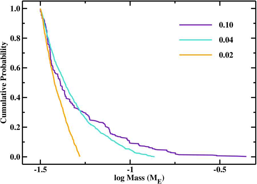
Figure 11: Mass distributions at 3 Myr for calculations with ensembles of Pluto-mass planetesimals. The legend indicates the initial disk mass in $\rm M_{\odot}$. The maximum planet mass scales with the disk mass. For planets with masses exceeding 10 $\rm M_{\oplus}$, the cumulative probability is roughly a power law, $p\propto M_{P}^{-\beta}$. Less massive disks have steeper probability distributions. Disks with initial masses $M_{d.0}\lesssim$ 0.01 $\rm M_{\odot}$ do not produce 10 $\rm M_{\oplus}$ planets.

Figure 11 shows the mass distributions for these calculations at 3 Myr. Independent of $\alpha$, the maximum planet mass scales with the initial disk mass as

$$M_{max}\approx 0.5~{}{\rm M_{\oplus}}\ \left(\frac{M_{d,0}}{0.1~{}M_{\odot}}\right)^{-1.5}~{}.$$ (29)

Because the most massive planets result from several rare collisions, the median mass is much smaller, $\sim$ 0.05 $\rm M_{\oplus}$ for disks with $M_{d,0}\approx$ 0.02–0.1 $\rm M_{\odot}$. Disks with smaller initial masses cannot produce planets more massive than $\sim$ 0.01 $\rm M_{\oplus}$.

For massive disks, the mass distribution is roughly a power law, with a cumulative probability $p\propto m^{-\beta}$. Our results suggest that more massive disks have shallower power laws, with $\beta\approx$ 2 for $M_{d,0}=$ 0.1 $\rm M_{\odot}$ and $\beta\approx$ 4 for $M_{d,0}=$ 0.04 $\rm M_{\odot}$.

These calculations demonstrate that disks composed of Pluto-mass objects can never become gas giant planets. This result is not surprising. For a disk with surface density $\Sigma$, the accretion time is roughly $t\propto RP/\Sigma$, where $P$ is the orbital period (e.g. Lissauer, 1987; Goldreich, Lithwick, & Sari, 2004). Thus, large planetesimals grow more slowly than small planetesimals (see also Kenyon & Bromley, 2008). In the limit of large objects growing without gravitational focusing, equation (56) of Goldreich, Lithwick, & Sari (2004) suggests that an ensemble of Plutos can produce 10 $\rm M_{\oplus}$ objects in 200–400 Myr at 3 AU. Our numerical simulations confirm this long growth time.

4.2 Calculations with Pebbles and a few Plutos

Disks composed of a few Plutos and many pebbles evolve rapidly. For a model with $M_{d,0}$ = 0.1 $\rm M_{\odot}$, $R_{d,0}$ = 30 AU, and $\alpha=10^{-3}$, it takes $\sim$ 1.5–1.8 Myr to promote the first object into the $N$-body code. Within 0.5 Myr, another 10–15 objects reach the promotion mass of $3\times 10^{26}$ g. These objects have small atmospheres; they rapidly accrete the remaining pebbles in their feeding zones. It typically takes $\sim$ 0.2 Myr for protoplanets to reach masses of 1–2 $\rm M_{\oplus}$ and another 0.2–0.5 Myr to begin to accrete gas from the disk. Within a total evolution time of 2.5–3 Myr, some protoplanets grow into gas giant planets.

The disk viscosity parameter $\alpha$ sets the timescale for the early portions of this evolution. In calculations with $\alpha=10^{-2}$, the timescale to produce the first $N$-body is $\sim$ 2 Myr, much longer than the 0.2–0.4 Myr timescale for calculations with $\alpha=10^{-4}-10^{-5}$. In these models, $\alpha$ sets the scale height of the pebbles (equation (21)). Gravitational focusing factors grow with smaller scale heights; thus, the Pluto-mass seeds accrete pebbles more rapidly when $\alpha$ is small. Our results suggest that planets grow much more rapidly in disks with $\alpha\lesssim 10^{-4}$.

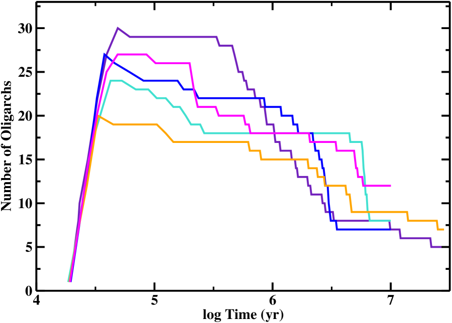
Figure 12: Time evolution of $N_{oli}$, the number of oligarchs with $M_{p}>3\times 10^{26}$, in models with $M_{d,0}$ = 0.1 $\rm M_{\odot}$, $R_{d,0}$ = 30 AU, and $\alpha=10^{-3}$. In these simulations, $N_{oli}$ rises as Pluto mass seeds rapidly accrete tiny pebbles, reaches a plateau when these seeds begin to accrete gas, and then falls as gas giant planets merge with other gas giants and smaller oligarchs. As gas giants achieve stable orbits, $N_{oli}$ stabilizes.

Stochastic processes are another feature of the evolution. In calculations with $\alpha=10^{-4}$, it takes $2-5\times 10^{4}$ yr to produce an ensemble of massive oligarchs (Kokubo & Ida, 1998) with $M_{p}\gtrsim 3\times 10^{26}$ g (Figure 12). For a large set of calculations with identical starting conditions, the random timing of oligarch formation and variations in accretion rates for each oligarch lead to a broad range in $N_{o,max}$, the maximum number of oligarchs. Often a rapidly accreting oligarch prevents a neighboring oligarch from accreting pebbles and reaching the promotion mass. Thus, calculations with small $N_{o,max}$ tend to have more massive oligarchs than calculations with large $N_{o,max}$.

Mergers of protoplanets are the final important feature of the growth of gas giant planets (see also Thommes et al., 2002; Kenyon & Bromley, 2006; Ida & Lin, 2010; Li et al., 2010). As protoplanets grow to masses of 5–10 $\rm M_{\oplus}$, their orbital separations are typically 10–20 Hill radii. Thus, mergers are rare. Once protoplanets start to accrete gas, their separations rapidly become smaller than 5–10 Hill radii. Strong dynamical interactions among pairs of protoplanets begin. Some interactions scatter protoplanets into the inner disk at 1–3 AU; others scatter protoplanets into the outer disk at $\gtrsim$ 30–100 AU (see also Marzari & Weidenschilling, 2002; Veras et al., 2009; Raymond et al., 2009a, 2009b, 2010). Throughout this chaotic growth phase, mergers rapidly deplete the number of growing protoplanets (Figure 12). Once the number of protoplanets reaches $\sim$ 5–10, planets have typical separations of $\gtrsim$ 10 Hill radii. Chaotic growth ends.

The timescale for chaotic growth varies from one calculation to the next (Figure 12). Sometimes, protoplanets are widely separated, grow slowly, and reach chaotic growth at late times (indigo and blue curves in Figure 12). When several closely packed protoplanets begin to accrete gas at roughly the same time, their growth initiates an early phase of chaotic growth (magenta and turquoise curves in Figure 12). In nearly all cases, chaotic growth ceases on timescales of 3–10 Myr.

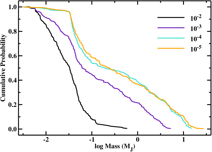
Figure 13: Mass distributions at 3 Myr for disks with $M_{d,0}$ = 0.1 $\rm M_{\odot}$, $R_{d,0}$ = 30 AU, and $\alpha$ as indicated in the legend. Disks with smaller $\alpha$ produce more massive gas giants. The median mass of gas giants ranges from $\sim$ 20 $\rm M_{\oplus}$ for $\alpha=10^{-2}$ to $\sim$ 0.25 $\rm M_{J}$ for $\alpha=10^{-5}$.

With growth rates sensitive to $\alpha$, the mass distributions of planets also depend on $\alpha$ (Figure 13). In calculations with $M_{d,0}$ = 0.1 $\rm M_{\odot}$ and $R_{d,0}$ = 30 AU, disks with small $\alpha$ produce a variety of gas giants, with masses ranging from 10 $\rm M_{\oplus}$ to 10–20 $\rm M_{J}$. Disks with larger and larger $\alpha$ yield smaller and smaller gas giants. For all $\alpha$, the probability of a given mass is roughly a power law, $p\propto M_{P}^{-n}$, with $n$ = 0.25–1. Thus, these calculations produce more Earth mass planets than Jupiter mass planets (see also Ida & Lin, 2005; Mordasini et al., 2009). The exponent in the power law depends on $\alpha$: models with smaller $\alpha$ produce broader probability distributions with smaller $n$.

For all $\alpha$, gas giants have a broad range of core masses. Although gas accretion begins when the core mass is 10 $\rm M_{\oplus}$, planets continue to accrete solid pebbles. During chaotic growth, protoplanets wander through a large range in orbital semimajor axis $a$, sweeping up (or scattering) pebbles and smaller oligarchs along their orbits. Mergers of two gas giants also augment the core mass. For disks with $M_{d,0}$ = 0.1 $\rm M_{\odot}$, core masses range from 10 $\rm M_{\oplus}$ to 100 $\rm M_{\oplus}$.

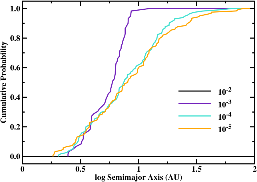
Figure 14: As in Fig. 13 for the semimajor axes of planets with masses larger than 1 $\rm M_{J}$. Disks with smaller $\alpha$ produce gas giants over a broader range of semimajor axes. The median semimajor axis ranges from $\approx$ 6 AU for $\alpha=10^{-3}$ to $\approx$ 8 AU for $\alpha=10^{-5}$. Disks with $\alpha=10^{-2}$ do not make massive gas giant planets.

Our calculations suggest that Jupiter mass or larger planets form throughout the disk (Figure 14). For $\alpha\lesssim 10^{-4}$, Jupiters achieve fairly stable orbits at semimajor axes $a_{J}\approx$ 2–30 AU. Although most 10 $\rm M_{\oplus}$ cores form at $a\sim$ 4–10 AU, dynamical interactions scatter protoplanets to $a\approx$ 1–3 AU and to $a\gtrsim$ 15–20 AU (see also Tsiganis et al., 2005). After the scattering events, these planets continue to accrete material and can grow to gas giant planets in their new orbits.

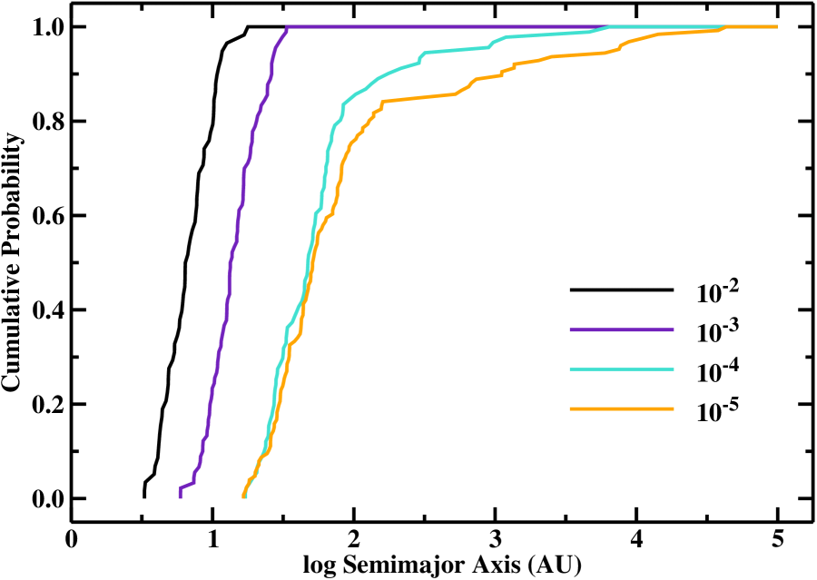
Figure 15: As in Fig. 14 for the semimajor axes of planets with masses between 15 $\rm M_{\oplus}$ and 1 $\rm M_{J}$. Disks with smaller $\alpha$ produce Neptune to Jupiter mass planets at larger semimajor axes. At 3 Myr, the median semimajor axis ranges from $\approx$ 6 AU for $\alpha=10^{-2}$ to $\approx$ 50 AU for $\alpha=10^{-5}$.

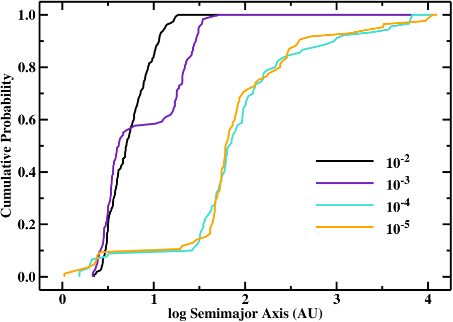
Figure 16: As in Fig. 14 for the semimajor axes of planets with masses 1–15 $\rm M_{\oplus}$. Disks with smaller $\alpha$ produce super-Earth mass planets over a broader range of semimajor axes. Super-Earths avoid regions near Jupiter mass planets. At 3 Myr, the median semimajor axis ranges from $\approx$ 5 AU for $\alpha=10^{-2}$ to $\approx$ 60 AU for $\alpha=10^{-5}$.

Planets with smaller masses have broader distributions of semimajor axes than massive gas giants. For convenience, we divide lower mass planets into ‘Saturns’ with masses of 15 $\rm M_{\oplus}$ to 1 $\rm M_{J}$ and ‘super-Earths’ with masses of 1–15 $\rm M_{\oplus}$. For large $\alpha\sim$ $10^{-3}-10^{-2}$, Saturn-mass planets are often the most massive planet in the system and have orbits with $a_{S}\approx$ 3–30 AU (Figure 15). When $\alpha$ is small, $\approx 10^{-4}-10^{-5}$, Saturns are scattered into orbits with $a_{S}\gtrsim$ 100 AU, well outside those of Jupiter-mass planets. A few Saturn-mass planets are ejected from the system. Super-Earths have even broader distributions of semimajor axis. All super-Earths avoid regions close to gas giant planets (Figure 16). Although a few super-Earths are scattered into the inner disk, most are scattered into the outer disk. Many super-Earths are ejected.

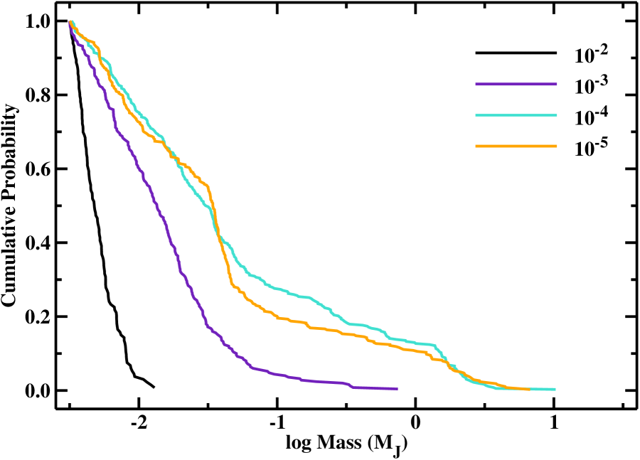
Figure 17: Mass distributions at 3 Myr for disks with $M_{d,0}$ = 0.04 $\rm M_{\odot}$, $R_{d,0}$ = 30 AU, and $\alpha$ as indicated in the legend. Disks with smaller $\alpha$ produce more massive gas giants. The median mass of planets ranges from $\sim$ 1.5 $\rm M_{\oplus}$ for $\alpha=10^{-2}$ to $\sim$ 20 $\rm M_{\oplus}$ for $\alpha=10^{-5}$.

Lower mass disks produce correspondingly lower mass planets. Figure 17 shows predicted mass distributions for planets in a disk with $M_{d,0}$ = 0.04 $\rm M_{\odot}$. Disks with $\alpha\gtrsim 10^{-3}$ fail to produce Jupiter mass planets; disks with smaller $\alpha$ rarely produce 3–20 $\rm M_{J}$ planets. The semimajor axes of these planets are much more concentrated towards the central star. The rare Jupiter mass planets lie within 10 AU; Saturn mass planets occupy 3–30 AU. Super-Earths occupy the largest range in $a$, with $a_{SE}\approx$ 1–100 AU.

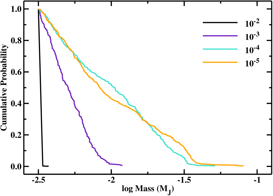
Figure 18: As in Figure 17 for disks with $M_{d,0}$ = 0.02 $\rm M_{\odot}$. Note the change of scale for the abscissa compared to other figures. The median mass ranges from $\sim$ 1 $\rm M_{\oplus}$ for $\alpha=10^{-2}$ to $\sim$ 6 $\rm M_{\oplus}$ for $\alpha=10^{-5}$.

Our results suggest that lower mass disks fail to produce gas giants for any $\alpha$. In disks with $M_{d,0}$ = 0.02 $\rm M_{\odot}$ (Figure 18), disks with small $\alpha$ sometimes produce ice giants with $M_{p}\approx$ 15–30 $\rm M_{\oplus}$. However, most planets in these simulations are super-Earths with $M_{p}\approx$ 1–15 $\rm M_{\oplus}$. Nearly all of these planets lie at small semimajor axes, $a_{SE}\approx$ 3–10 AU.

Finally, these calculations produce a diverse set of multi-planet systems (Table 1). For any $M_{d,0}$, disks with smaller $\alpha$ yield a larger frequency of systems with at least two planets. Defining $M_{p,max}$ as the maximum planet mass, planetary systems with smaller $M_{p,max}$ tend to have more planets. Systems with 4 Jupiter mass planets are rare: 5–10% among 0.1 $\rm M_{\odot}$ disks and less than 1% among lower mass disks. Systems with 4–10 super-Earths are relatively common, with frequencies of 70% or more among 0.01–0.02 $\rm M_{\odot}$ disks.

5 SUMMARY

The current version of our hybrid code now includes all of the necessary physics to calculate the formation of gas giant planets from an input ensemble of planetesimals in an evolving gaseous disk. The new features of the code include

1. the time evolution of a viscous disk with mass loss from photoevaporation and gas giant planet formation,

2. the atmospheric structure of planets with $R\approx$ 0.001–10 $\rm R_{\oplus}$ with an algorithm to calculate the enhanced radius of a planet and the accretion of small dust grains,

3. gas accretion onto Earth-mass icy cores,

4. the time evolution of the radius and luminosity of gas giants,

5. the gravitational potential of a massive gaseous disk and its impact on the orbits of planets, and

6. the gravitational perturbation of (i) $N$-bodies on a disk of planetesimals and (ii) a disk of massive planetesimals on $N$-bodies.

The new hybrid code accurately treats the migration of planets through a disk of massive planetesimals. Simulations with isolated planets reproduce the results of Kirsh et al. (2009), where the planet migrates inwards through undisturbed planetesimals. Simulations with multiple planets reproduce the results of Hahn & Malhotra (1999). These two examples illustrate the importance of the dynamical state of the planetesimals. In the simulations for Fig. 10, the initial environment of the planetesimals orbiting near Neptune is similar to the initial conditions near the single planet in the calculations for Fig. 8–9. Yet, the migration rates in the two cases differ in magnitude and sign. Bromley & Kenyon (2011) investigate this phenomenon in more detail.

To begin to understand the orbital migration of ensembles of gas giants in an evolving, gaseous disk, we consider a new ‘type 0’ migration mechanism. Here, the semimajor axes of planets evolve as the disk mass changes. Although the degree of migration is limited by the ratio of the mass of the disk to the mass of the host star, modest inward or outward migration is possible. Because angular momentum is invariant, the sign of the migration depends on the mode of mass and angular momentum loss. In systems that lose mass by disk accretion, migration is inward. Mass loss by photoevaporation may lead to outward migration. Both modes may be important in establishing pairs of planets in resonant orbits (e.g., as in Holman et al., 2010).

To explore the ability of our code to simulate the formation of gas giant planets, we consider the evolution of planetesimals in disks with a variety of initial masses and viscosity parameters. Disks of Pluto-mass planetesimals cannot form gas giants. For disks with initial masses of 0.1 $\rm M_{\odot}$ and all values of $\alpha$, the maximum planet mass is roughly 0.5 $\rm M_{\oplus}$. Lower mass disks produce substantially lower mass planets.

Disks composed of 0.1–1 cm pebbles and a few Pluto-mass seeds can produce Jupiter mass planets on short timescales. Our results demonstrate that the properties of planetary systems depend on the initial disk mass $M_{d,0}$ and the viscosity parameter $\alpha$ (Figure 19).

1. More massive disks produce more massive planets on more rapid timescales. In disks with $M_{d,0}$ = 0.1 $\rm M_{\odot}$, Jupiter-mass planets are common at 1–2 Myr. In lower mass disks, super-Earths and Saturns form in 2–3 Myr. The timescales are similar to the observed lifetimes, $\sim$ 1–3 Myr, of circumstellar disks around low mass pre-main sequence stars (e.g., Haisch, Lada, & Lada, 2001; Kennedy & Kenyon, 2009; Mamajek, 2009).

2. Disks with larger $\alpha$ form lower mass planets. In disks with $\alpha=10^{-2}-10^{-3}$, Jupiters form rarely; Saturns and Super-Earths are common. In disks with $\alpha=10^{-4}-10^{-5}$, planetary systems with 2 or more Jupiters are common. This result suggests that Jupiters probably form more often in disks with ‘dead zones,’ regions where the disk viscosity parameter is much lower than the rest of the disk (e.g., Matsumura et al., 2009).

3. The derived distributions of planet mass spans the range of known exoplanets. For planets with $M_{P}\approx$ 0.03–10 $\rm M_{J}$, disks with $M_{d,0}$ = 0.1 $\rm M_{\odot}$ and $\alpha$ = $10^{-5}-10^{-4}$ yield a roughly power law probability distribution $dp/d~{}{\rm log}~{}M_{p}$ $\propto M_{P}^{-n}$ with $n$ = 0.20–0.25. Disks with $\alpha$ = $10^{-2}$ have a much steeper relation, with $n\approx$ 0.8–0.9. Known exoplanets have an intermediate frequency distribution, with $n\approx$ 0.48 (Howard et al., 2010). Thus, simulations with small (large) $\alpha$ produce relatively fewer (more) super-Earths and Saturns than observed in real systems. If real protostellar disks have a range of $\alpha$ that includes our small and large $\alpha$ regimes, some mix of $\alpha$ can probably ‘match’ the observations. However, including other physical processes – such as migration and photoevaporation – will change the slopes of the mass-frequency relation (see, for example, Ida & Lin, 2005; Mordasini et al., 2009). Thus, detailed comparison with observations is premature.

4. The derived distribution of semimajor axes is roughly linear in $a$ over 3–30 AU. Scattering leads to a few gas giants at 1–3 AU and at 30–100 AU. Without a treatment of migration, our predicted distribution of semimajor axes cannot hope to match observations. However, our ability to scatter gas giants out to 30–100 AU may allow core accretion models to produce systems similar to HR 8799 (Marois et al., 2008).

5. These calculations often produce planetary systems with 2–10 planets. Planetary systems with multiple planets usually contain super-Earths, sometimes contain Saturns, and rarely contain Jupiters. Current observations suggest that roughly 10% of all planetary systems have two or more gas giant and/or ice giant planets (Gould et al., 2010, also statistics at exoplanet.eu and exoplanets.org). However, some planetary systems may have as many as 7 super-Earth or ice giant planets (e.g., HD10180; Lovis et al., 2010). Given current poor constraints on initial disk mass and viscosity in protostellar disks, our results can ‘match’ both of these observations.

6. Jupiter mass planets in these calculations have core masses of 10–100 $\rm M_{\oplus}$. Once icy 10 $\rm M_{\oplus}$ cores start to accrete gas, they continue to accrete solids from the disk. Mergers with other gas giants also augment the core mass. When mergers between growing protoplanets are rare, planets have modest core masses, 10–20 $\rm M_{\oplus}$. When mergers between icy cores are common, core masses approach 100 $\rm M_{\oplus}$. Multiple mergers of growing protoplanets may account for the large heavy element abundances in HD 149026b and other exoplanets (Burrows et al., 2007; Fortney et al., 2009).

These results are encouraging. Our simple set of initial calculations accounts for the observed range of planet masses and for some of the observed range of semimajor axes. The derived power law slopes for the frequency of planet masses bracket the observations. Compared with real planetary systems, the calculations probably produce too many multi-planet systems.

Adding more realism (e.g., migration, photoevaporation, etc) to our simulations will allow us to improve our understanding of the processes that lead to ice/gas giant planet formation. Integrating orbits past $\sim$ 10 Myr will enable robust comparisons between the properties of real and simulated planetary systems. Together with improved observations of protoplanetary disks and better data for exoplanets, numerical simulations like ours should lead to clear tests for the core accretion theory of planet formation.

Appendix A The gravitational potential of an unperturbed disk

If the gaseous protostellar disk is extended, thin, and axisymmetric, our code can treat the gravitational effect of the disk on the planets. We estimate the gravitational potential produced by a geometrically thin, axisymmetric disk in two ways. The first method is based on an analytical inversion of the Poisson equation from an expansion of the surface density $\Sigma$ into Bessel functions. The results are simple expressions for the potential, valid for 2D disks of large spatial extent and a surface density that is a pure power-law in orbital distance. The second method employs brute force, using a direct numerical integration of the mass density over a geometrically thin, axisymmetric 3D disk. This approach gives the potential associated with an arbitrary surface density profile, with the advantage of generalizability at the expense of computational load.

The analytical approach for estimating the disk potential as it acts on a unit-mass particle takes advantage of solutions to the Laplace equation that are linear combinations of Bessel functions of the first kind, $J_{0}(x)$ (Binney & Tremaine, 1987, §2.6)

$$\Phi_{d}(R,z)=\int_{0}^{\infty}S(k)J_{0}(kR)e^{-k|z|}dk,$$ (A1)

where $S(k)$ is a density function. The exponential with the discontinuous first derivative at $z=0$ generates a $\delta$ function in the 3D density at the disk midplane upon application of the Laplace operator. Gauss’s law relates this potential to the surface density. A closed, pillbox-shaped surface with a unit-area cross-section that straddles the disk midplane has a gravitational field flux $-2d\Phi_{d}/dz$, and encloses a mass $\Sigma$. Gauss’s law sets the flux equal to $4\pi G$ times the enclosed mass, hence

$$\Sigma(R)=-\frac{1}{2\pi G}\int_{0}^{\infty}S(k)J_{0}(kR)kdk.$$ (A2)

The integral is a Hankel transform (to within a multiplicative constant), and we identify $S(k)$ and $\Sigma(R)$ as transform pairs, with

$$S(k)=-2\pi G\int_{0}^{\infty}\Sigma(R)J_{0}(kR)RdR.$$ (A3)

We now assume that the surface density $\Sigma(R)$ is a power law in $R$ with an arbitrarily large radial extent, i.e., ${R_{\rm in}}\rightarrow 0$ and ${R_{\rm out}}\rightarrow\infty$. In this case,

$$\Sigma(a)=\Sigma_{0}(R_{0}/R)^{-{\rm n}}$$ (A4)

and

$$S(k)=-2\pi G\Sigma_{0}R_{0}^{{\rm n}}k^{{\rm n}-2}\int_{0}^{\infty}q^{1-{\rm n}}J_{0}(q)dq\ .$$ (A5)

We impose the condition that $1/2<{\rm n}<2$ so that the mass in the disk is finite inside a finite radius, with the lower limit set so that the integral in equation A5 is well-defined. This integral is of the form

$$I_{n}(\mu) = \int_{0}^{\infty}x^{\mu}J_{n}(x)dx$$ (A6)

$$= 2^{\mu}\frac{{\rm n}(\frac{n+1+\mu}{2})}{{\rm n}(\frac{n+1-\mu}{2})}$$ (A7)

$$= \frac{1}{I_{n}(-\mu)}\ ,$$ (A8)

$$S(k)\approx-2\pi G\Sigma_{0}R_{0}^{{\rm n}}k^{{\rm n}-2}I_{0}(2-{\rm n})\ .$$ (A9)

Similarly, the potential in the disk midplane is

$$\Phi_{d}(R)=-2\pi G\Sigma_{0}R\left(\frac{R}{R_{0}}\right)^{-{\rm n}}I_{0}(1-{\rm n})I_{0}({\rm n}-2),$$ (A10)

although this expression is formally valid only for $1<{\rm n}<2$. The radial component of the acceleration, $a_{r}$, is not subject to this formal restriction on ${\rm n}$; it obtains from the derivative of $\Phi_{d}$ with respect to $R$, along with the identity $dJ_{0}(x)/dx=-J_{1}(x)$:

$$a_{r}=-2\pi G\Sigma_{0}I_{0}(1-{\rm n})I_{1}(1-{\rm n})\left(\frac{R}{a_{0}}\right)^{-{\rm n}},$$ (A11)

which is exact in the midplane of an infinitely extended disk.

To illustrate results from the above analysis, we give the following examples of the potential and radial acceleration for a few power-law surface density profiles:

$$\begin{array}[]{lll}{\rm n}=0.6:&\Phi_{d}=2.8\pi G\Sigma_{0}R_{0}^{0.6}R^{0.4}&\ \ \ \hfil\hfil\break a_{r}=-1.1\pi G\Sigma_{0}(R/R_{0})^{-0.6}\vskip 6.0pt plus 2.0pt minus 2.0pt\\ {\rm n}=1.0&\Phi_{d}=2\pi G\Sigma_{0}R_{0}\log(R)+{\rm const}&\ \ \ \hfil\hfil\break a_{r}=-2\pi G\Sigma_{0}R_{0}/R\vskip 6.0pt plus 2.0pt minus 2.0pt\\ {\rm n}=1.5&\Phi_{d}=-8.8\pi G\Sigma_{0}R_{0}^{1.5}R^{-0.5}&\ \ \ \hfil\hfil\break a_{r}=-4.4\pi G\Sigma_{0}(R/R_{0})^{-1.5}\end{array}$$ (A12)

As long as the orbital distance $R$ approximately satisfies ${R_{\rm in}}<0.1R$ and $10R<{R_{\rm out}}$, these expressions hold for disks of finite extent.

As an alternative to the analytical method, which is limited in terms of the functional form of $\Sigma(R)$, we take a numerical approach to directly integrate the mass in the disk to get the gravitational potential:

$$\Phi_{d}(\vec{r},t)=\int_{R_{\rm in}}^{R_{\rm out}}\int_{-\pi}^{\pi}\frac{dRd\varphi R\Sigma(R,t)}{\sqrt{(}r_{\perp}^{2}+z^{2}+h^{2}+R^{2}-2r_{\perp}R\cos(\varphi)},$$ (A13)

where position $\vec{r}$ relative to the host star is in cylindrical coordinates, $(r_{\perp},\varphi,z)$. The variable $h$ is a softening parameter, which formally eliminates the density singularity in the disk midplane by making the 2D disk behave as if it has some finite thickness. From the Poisson equation, we find that the effective vertical density profile is approximately Gaussian, with a scale height of $\sigma\sim h$. Here we take $h=0.01$ AU; in what follows, the results do not strongly depend on this choice.

The next step is to integrate eq. (A13) numerically; the radial integration can be solved analytically, but integrating over the angular coordinate $\varphi$ requires a Chebyshev-Legendre quadrature scheme. The number of sample points $n$ in our quadrature scheme is variable; we increase $n$ by a factor of four successively until the relative change in the result from one iteration to the next is below an error tolerance of $10^{-7}$. For the integrands encountered here, the result is much more accurate than the error tolerance suggests, because the quadrature scheme typically converges quadratically or better.

Compared to with evaluating the $1/r$ potential from the central star, this method is computationally expensive. To alleviate this problem, we limit the calculations to the disk midplane—a reasonable approximation since the orbital inclination of planets not entrained in the gas is typically less than the disk scale height. Then we evaluate the potential at a set of logarithmically spaced points in orbital separation and interpolate with cubic splines. The computational load then reduces to $O(10)$ arithmetic operations.

Appendix B Time-varying disk mass (“type 0” migration)

When the disk mass is removed from the planetary system by photoevaporation or some other slow process, the time-varying disk mass can produce a radial migration of a planet’s orbit. Angular momentum is conserved. For example, the product of the semimajor axis $a$ and the central star mass $M$ remains constant when the star itself loses mass. For low-eccentricity orbits, the conserved quantity is equal to $a^{3}a_{r}$, where $a_{r}$ is the acceleration on the body from both the star and gaseous disk. If the disk mass—but not the stellar mass—varies in time,

$$a(t) = a(0)\frac{1+2\pi\Sigma_{0}/MI_{0}(1-{\rm n})I_{1}(1-{\rm n})a_{0}^{{\rm n}}a(0)^{2-{\rm n}}}{1+M2\pi\Sigma_{0}/MI_{0}(1-{\rm n})I_{1}(1-{\rm n})a_{0}^{\rm n}a(t)^{2-{\rm n}}e^{-t/\tau}}$$ (B1)

$$\approx \hfil\hfil\break\left[1+2\pi\Sigma_{0}/MI_{0}(1-{\rm n})I_{1}(1-{\rm n})a_{0}^{{\rm n}}a(0)^{2-{\rm n}}\right]\ \ \ \ (t\gg\tau)\,.$$ (B2)

Setting ${\rm n}=1$ and taking the limit of $t\rightarrow\infty$, the maximum change in orbital distance for a planet at 1 AU in an evaporating disk with initial surface density $\Sigma 0=3000$ g/cm² is roughly 1%. If a disk with the same mass is more centrally concentrated (${\rm n}=1.5$), this number is roughly an order of magnitude higher. For planets farther out in the disk, the maximum change is much larger, $\sim$ 5% at 10 AU and $\sim$ 10% at 30 AU.

Table 1: Frequency of Multi-Planet Systems

		Number of Planets
$\alpha$	Mass Key	0	1	2	3	4	5	6	7	8
$M_{d,0}$ = 0.1 $\rm M_{\odot}$
$10^{-2}$	S	0.30	0.16	0.30	0.16	0.05	0.00	0.00	0.00	0.00
$10^{-3}$	J	0.30	0.35	0.35	0.00	0.00	0.00	0.00	0.00	0.00
$10^{-4}$	J	0.00	0.00	0.19	0.70	0.11	0.00	0.00	0.00	0.00
$10^{-5}$	J	0.00	0.02	0.25	0.68	0.05	0.00	0.00	0.00	0.00
$M_{d,0}$ = 0.04 $\rm M_{\odot}$
$10^{-2}$	SE	0.00	0.00	0.33	0.37	0.28	0.02	0.00	0.00	0.00
$10^{-3}$	S	0.47	0.37	0.16	0.00	0.00	0.00	0.00	0.00	0.00
$10^{-4}$	J	0.18	0.65	0.17	0.00	0.00	0.00	0.00	0.00	0.00
$10^{-5}$	J	0.06	0.55	0.35	0.04	0.00	0.00	0.00	0.00	0.00
$M_{d,0}$ = 0.02 $\rm M_{\odot}$
$10^{-2}$	SE	0.97	0.03	0.00	0.00	0.00	0.00	0.00	0.00	0.00
$10^{-3}$	SE	0.00	0.00	0.02	0.21	0.33	0.37	0.07	0.00	0.00
$10^{-4}$	S	0.97	0.03	0.00	0.00	0.00	0.00	0.00	0.00	0.00
$10^{-5}$	S	0.91	0.09	0.00	0.00	0.00	0.00	0.00	0.00	0.00
$M_{d,0}$ = 0.01 $\rm M_{\odot}$
$10^{-2}$	SE	1.00	0.00	0.00	0.00	0.00	0.00	0.00	0.00	0.00
$10^{-3}$	SE	0.98	0.02	0.00	0.00	0.00	0.00	0.00	0.00	0.00
$10^{-4}$	SE	0.00	0.00	0.00	0.31	0.28	0.28	0.13	0.00	0.00
$10^{-5}$	SE	0.00	0.00	0.00	0.00	0.00	0.12	0.31	0.29	0.28

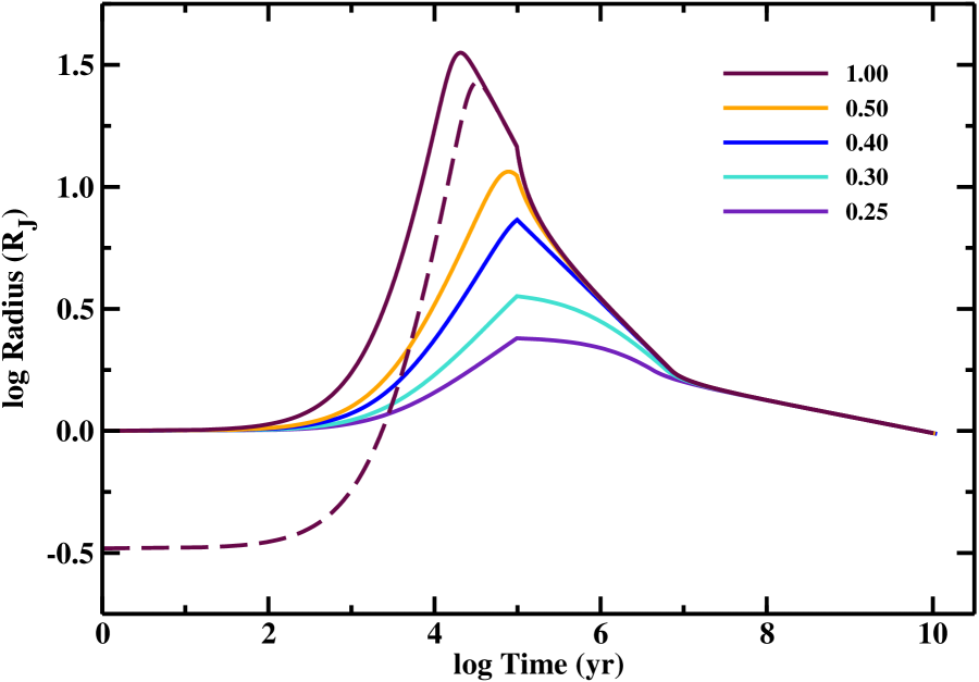
Figure 5: As in Figure 4 for the radius of the planet. Planets that accrete hotter gas grow to larger radii.

Figure 8: The evolution of eccentricity in units of Hill radii as a function of semimajor axis during planet migration. The three panels show snapshots at the indicated times as a 2 $\rm M_{\oplus}$ planet travels through a sea of planetesimals, similar to Kirsh et al. (2009) — $\Sigma\sim 1/a$, normalized to 1.2 g cm^-2 at 25 AU, and extending from 14.5 AU to 35.5 AU. The blob of particles in each panel ($\sim$ 25 AU at $10^{4}$ yr, $\sim$ 24 AU at $3\times 10^{4}$ yr, and $\sim$ 22 AU at $6\times 10^{4}$ yr) indicates the location of the planet.

Figure 9: The evolution of the semimajor axis of a planet in the planetesimal disk from Figure 8. The initially flat migration profile stems from “inertia” associated with planetesimals in the co-orbital zone (the blobs of particles in Fig. 8, which diffuse away in time). After the planet scatters these particles out of its orbit, fast migration begins.

Figure 10: Migration of the major planets in a planetesimal disk. The planets, with their present-day masses, evolve from an initially compact configuration as a result of interactions with 1000 planetesimals, each with a mass of 0.1 $\rm M_{\oplus}$, uniformly distributed in semimajor axis from 10 AU to 50 AU. In contrast to the behavior of the single planet in Fig. 9, interactions between planetesimals and multiple planets cause the outward migration of Neptune and Uranus (see Hahn & Malhotra, 1999).

Figure 19: Outcomes of planet formation simulations. The regions indicate the maximum masses of planets as a function of the initial disk mass, $M_{d,0}$, and the disk viscosity parameter, $\alpha$.

References

- (1)
- Adachi et al. (1976) Adachi, I., Hayashi, C., & Nakazawa, K. 1976, Progress of Theoretical Physics 56, 1756
- Alexander et al. (2006) Alexander, R. D., Clarke, C. J., & Pringle, J. E. 2006, MNRAS, 369, 216
- Alexander & Armitage (2007) Alexander, R. D., & Armitage, P. J. 2007, MNRAS, 375, 500
- Alexander & Armitage (2009) Alexander, R. D., & Armitage, P. J. 2009, ApJ, 704, 989
- Alibert et al. (2005) Alibert, Y., Mordasini, C., Benz, W., & Winisdoerffer, C. 2005, A&A, 434, 343
- Andrews & Williams (2005) Andrews, S. M., & Williams, J. P. 200in5, ApJ, 631, 1134
- Andrews & Williams (2007) Andrews, S. M., & Williams, J. P. 2007a, ApJ, 659, 705
- Andrews et al. (2009) Andrews, S. M., Wilner, D. J., Hughes, A. M., Qi, C., & Dullemond, C. P. 2009, ApJ, 700, 1502
- Baraffe et al. (2003) Baraffe, I., Chabrier, G., Barman, T. S., Allard, F., & Hauschildt, P. H. 2003, A&A, 402, 701
- Baraffe et al. (2008) Baraffe, I., Chabrier, G., & Barman, T. 2008, A&A, 482, 315
- Baraffe et al. (2009) Baraffe, I., Chabrier, G., & Gallardo, J. 2009, ApJ, 702, L27
- Bath & Pringle (1981) Bath, G. T., & Pringle, J. E. 1981, MNRAS, 194, 967
- Bath & Pringle (1982) Bath, G. T., & Pringle, J. E. 1982, MNRAS, 199, 267
- Benz & Asphaug (1999) Benz, W., & Asphaug, E. 1999, Icarus, 142, 5
- Binney & Tremaine (1987) Binney, J., & Tremaine, S. 1987, Galactic Dynamics (Princeton, NJ, Princeton University Press)
- Birnstiel et al. (2009) Birnstiel, T., Dullemond, C. P., & Brauer, F. 2009, A&A, 503, L5
- Borucki et al. (2010) Borucki, W., et al. 2010, arXiv:1006.2799
- Brauer et al. (2008) Brauer, F., Henning, T., & Dullemond, C. P. 2008, A&A, 487, L1
- Bromley & Kenyon (2006) Bromley, B., & Kenyon, S. J. 2006, AJ, 131, 2737
- Bromley & Kenyon (2011) Bromley, B., & Kenyon, S. J. 2011, ApJ, submitted (arXiv: 1101:4025)
- Burrows et al. (1997) Burrows, A., et al. 1997, ApJ, 491, 856
- Burrows et al. (2007) Burrows, A., Hubeny, I., Budaj, J., & Hubbard, W. B. 2007, ApJ, 661, 502
- Chabrier et al. (2007) Chabrier, G., Baraffe, I., Selsis, F., Barman, T. S., Hennebelle, P., & Alibert, Y. 2007, Protostars and Planets V, 623
- Chambers (2006) Chambers, J. 2006, Icarus, 180, 496
- Chambers (2008) Chambers, J. 2008, Icarus, 198, 256
- Chambers (2009) Chambers, J. E. 2009, ApJ, 705, 1206
- Chiang & Goldreich (1997) Chiang, E. I., & Goldreich, P. 1997, ApJ, 490, 368
- Chiang & Youdin (2010) Chiang, E., & Youdin, A. N. 2010, Annual Review of Earth and Planetary Sciences, 38, 493
- Cox (2000) Cox, A. N. 2000, Allen’s Astrophysical Quantities, Fourth edition, New York, AIP Press
- Cumming et al. (2008) Cumming, A., Butler, R. P., Marcy, G. W., Vogt, S. S., Wright, J. T., & Fischer, D. A. 2008, PASP, 120, 531
- Currie et al. (2007) Currie, T., Kenyon, S. J., Balog, Z., Bragg, A., & Tokarz, S. 2007, ApJ, 669, L33
- Currie et al. (2009) Currie, T., Lada, C. J., Plavchan, P., Robitaille, T. P., Irwin, J., & Kenyon, S. J. 2009, ApJ, 698, 1
- Cuzzi et al. (2008) Cuzzi, J. N., Hogan, R. C., & Shariff, K. 2008, ApJ, 687, 1432
- D’Alessio et al. (1998) D’Alessio, P., Canto, J., Calvet, N., & Lizano, S. 1998, ApJ, 500, 411
- D’Angelo et al. (2010) D’Angelo, G., Durisen, R. H., & Lissauer, J. J. 2010, arXiv:1006.5486
- D’Angelo & Lubow (2008) D’Angelo, G., & Lubow, S. H. 2008, ApJ, 685, 560
- Dodson-Robinson et al. (2008) Dodson-Robinson, S. E., Bodenheimer, P., Laughlin, G., Willacy, K., Turner, N. J., & Beichman, C. A. 2008, ApJ, 688, L99
- Duncan, Levison, & Lee (1998) Duncan, M. J., Levison, H. F., & Lee, M. H. 1998, AJ, 116, 2067
- Encke (1852) Encke, M. 1852, MNRAS, 13, 2
- Fortney et al. (2009) Fortney, J. J., Baraffe, I., & Militzer, B. 2009, arXiv:0911.3154
- Fukushima (1996) Fukushima, T. 1996, AJ, 112, 1263
- Garaud (2007) Garaud, P. 2007, ApJ, 671, 2091
- Gladman (1993) Gladman, B. 1993, Icarus, 106, 247
- Goldreich, Lithwick, & Sari (2004) Goldreich, P., Lithwick, Y., & Sari, R. 2004, ARA&A, 42, 549
- Goldreich & Tremaine (1980) Goldreich, P., & Tremaine, S. 1980, ApJ, 241, 425
- Gould et al. (2010) Gould, A., et al. 2010, ApJ, 720, 1073
- Greenzweig & Lissauer (1990) Greenzweig, Y., & Lissauer, J. J. 1990, Icarus, 87, 40
- Gullbring et al. (1998) Gullbring, E., Hartmann, L., Briceno, C., & Calvet, N. 1998, ApJ, 492, 323
- Haisch, Lada, & Lada (2001) Haisch, K., Lada, E. A., & Lada, C. J. 2001, ApJ, 553, 153
- Hahn & Malhotra (1999) Hahn, J. M., & Malhotra, R. 1999, AJ, 117, 3041
- Hartmann et al. (1998) Hartmann, L., Calvet, N., Gullbring, E., & D’Alessio, P. 1998, ApJ, 495, 385
- Hartmann et al. (1997) Hartmann, L., Cassen, P., & Kenyon, S. J. 1997, ApJ, 475, 770
- Helled et al. (2008) Helled, R., Podolak, M., & Kovetz, A. 2008, Icarus, 195, 863
- Holman et al. (2010) Holman, M. J., et al. 2010, Science, 330, 51
- Hori & Ikoma (2010) Hori, Y., & Ikoma, M. 2010, ApJ, 714, 1343
- Howard et al. (2010) Howard, A. W., et al. 2010, Science, 330, 653
- Hubickyj et al. (2005) Hubickyj, O., Bodenheimer, P., & Lissauer, J. J. 2005, Icarus, 179, 415
- Hueso & Guillot (2005) Hueso, R., & Guillot, T. 2005, A&A, 442, 703
- Ida et al. (2000) Ida, S., Bryden, G., Lin, D. N. C., & Tanaka, H. 2000, ApJ, 534, 428
- Ida & Lin (2005) Ida, S., & Lin, D. N. C. 2005, ApJ, 626, 1045
- Ida & Lin (2010) Ida, S., & Lin, D. N. C. 2010, ApJ, 719, 810
- Ida & Makino (1992) Ida, S., & Makino, J. 1992, Icarus, 96, 107
- Ikoma et al. (2000) Ikoma, M., Nakazawa, K., & Emori, H. 2000, ApJ, 537, 1013
- Inaba & Ikoma (2003) Inaba, S., & Ikoma, M. 2003, A&A, 410, 711
- Isella et al. (2009) Isella, A., Carpenter, J. M., & Sargent, A. I. 2009, ApJ, 701, 260
- Kary et al. (1993) Kary, D. M., Lissauer, J. J., & Greenzweig, Y. 1993, Icarus, 106, 288
- Kennedy & Kenyon (2008) Kennedy, G. M., & Kenyon, S. J. 2008, ApJ, 673, 502
- Kennedy & Kenyon (2009) Kennedy, G. M., & Kenyon, S. J. 2009, ApJ, 695, 1210
- Kenyon & Bromley (2001) Kenyon, S. J., & Bromley, B. C. 2001, AJ, 121, 538
- Kenyon & Bromley (2004a) Kenyon, S. J., & Bromley, B. C., 2004a, AJ, 127, 513
- Kenyon & Bromley (2004b) Kenyon, S. J., & Bromley, B. C., 2004b, ApJ, 602, L133
- Kenyon & Bromley (2004c) Kenyon, S. J., & Bromley, B. C., 2004c, AJ, 128, 1916
- Kenyon & Bromley (2006) Kenyon, S. J., & Bromley, B. C. 2006, AJ, 131, 1837
- Kenyon et al. (2008) Kenyon, S. J., Bromley, B. C., O’Brien, D. C., & Davis, D. R. 2008, in The Solar System Beyond Neptune, edited by A. Barucci, H. Boehnhardt, D. Cruikshank, & A. Morbidelli, Tucson, Univ. of Arizona Press, p. 293
- Kenyon & Bromley (2008) Kenyon, S. J., & Bromley, B. C. 2008, ApJS, 179, 451
- Kenyon & Bromley (2009) Kenyon, S. J., & Bromley, B. C. 2009, ApJL, 690, L140
- Kenyon & Bromley (2010) Kenyon, S. J., & Bromley, B. C. 2010, ApJS, 188, 242
- Kenyon & Luu (1998) Kenyon, S. J., & Luu, J. X. 1998, AJ, 115, 2136
- Kenyon & Luu (1999) Kenyon, S. J., & Luu, J. X. 1999, AJ, 118, 1101
- Kinoshita, Yoshida, & Nakai (1991) Kinoshita, H., Yoshida, H., & Nakai, H. 1991, Celestial Mechanics and Dynamical Astronomy, 50, 59
- Kirsh et al. (2009) Kirsh, D. R., Duncan, M., Brasser, R., & Levison, H. F. 2009, Icarus, 199, 197
- Kobayashi & Tanaka (2010) Kobayashi, H. & Tanaka, H. 2010, Icarus, 206, 735
- Kokubo & Ida (1995) Kokubo, E. & Ida, S. 1995, Icarus, 114, 247
- Kokubo & Ida (1998) Kokubo, E., & Ida, S. 1998, Icarus, 131, 171
- Kretke & Lin (2007) Kretke, K. A., & Lin, D. N. C. 2007, ApJ, 664, L55
- Krivov et al. (2006) Krivov, A. V., Löhne, T., & Sremčević, M. 2006, A&A, 455, 509
- Laibe et al. (2008) Laibe, G., Gonzalez, J.-F., Fouchet, L., & Maddison, S. T. 2008, A&A, 487, 265
- Leinhardt et al. (2008) Leinhardt, Z. M., Stewart, S. T., & Schultz, P. H. 2008, in The Solar System Beyond Neptune, edited by A. Barucci, H. Boehnhardt, D. Cruikshank, & A. Morbidelli, Tucson, Univ. of Arizona Press, p. 195
- Leinhardt & Stewart (2009) Leinhardt, Z. M., & Stewart, S. T. 2009, Icarus, 199, 542
- Levison et al. (2007) Levison, H. F., Morbidelli, A., Gomes, R., & Backman, D. 2007, Protostars and Planets V, 669
- Levison et al. (2010) Levison, H. F., Thommes, E., & Duncan, M. J. 2010, AJ, 139, 1297
- Li et al. (2010) Li, S. L., Agnor, C. B., & Lin, D. N. C. 2010, ApJ, 720, 1161
- Lin et al. (1996) Lin, D. N. C., Bodenheimer, P., & Richardson, D. C. 1996, Nature, 380, 606
- Lin & Papaloizou (1979) Lin, D. N. C., & Papaloizou, J. C. B. 1979, MNRAS, 186, 799
- Lin & Papaloizou (1986) Lin, D. N. C., & Papaloizou, J. 1986, ApJ, 309, 846
- Lissauer (1987) Lissauer, J. J. 1987, Icarus, 69, 249
- Lissauer & Stevenson (2007) Lissauer, J. J., & Stevenson, D. J. 2007, Protostars and Planets V, 591
- Löhne et al. (2008) Löhne, T., Krivov, A. V., & Rodmann, J. 2008, ApJ, 673, 1123
- Lovis et al. (2010) Lovis, C. et al. 2010, A&A, submitted
- Lynden-Bell & Pringle (1974) Lynden-Bell, D., & Pringle, J. E. 1974, MNRAS, 168, 603
- Machida et al. (2010) Machida, M. N., Kokubo, E., Inutsuka, S.-I., & Matsumoto, T. 2010, MNRAS, 405, 1227
- Malhotra (1993) Malhotra, R. 1993, Nature, 365, 819
- Mamajek (2009) Mamajek, E. E. 2009, American Institute of Physics Conference Series, 1158, 3
- Marley et al. (2007) Marley, M. S., Fortney, J. J., Hubickyj, O., Bodenheimer, P., & Lissauer, J. J. 2007, ApJ, 655, 541
- Marois et al. (2008) Marois, C., Macintosh, B., Barman, T., Zuckerman, B., Song, I., Patience, J., Lafrenière, D., & Doyon, R. 2008, Science, 322, 1348
- Marzari & Weidenschilling (2002) Marzari, F., & Weidenschilling, S. J. 2002, Icarus, 156, 570
- Matsumura et al. (2009) Matsumura, S., Pudritz, R. E., & Thommes, E. W. 2009, ApJ, 691, 1764
- Mayor et al. (2009) Mayor, M., et al. 2009, A&A, 493, 639
- Mitchell & Stewart (2010) Mitchell, T. R., & Stewart, G. R. 2010, ApJ, 722, 1115
- Mizuno (1980) Mizuno, H. 1980, Progress of Theoretical Physics, 64, 544
- Mordasini et al. (2009) Mordasini, C., Alibert, Y., & Benz, W. 2009, A&A, 501, 1139
- Nelson et al. (2000) Nelson, R. P., Papaloizou, J. C. B., Masset, F., & Kley, W. 2000, MNRAS, 318, 18
- O’Brien & Greenberg (2003) O’Brien, D. P., & Greenberg, R. 2003, Icarus, 164, 334
- Ohtsuki (1992) Ohtsuki, K. 1992, Icarus, 98, 20
- Ohtsuki, Stewart, & Ida (2002) Ohtsuki, K., Stewart, G. R., & Ida, S. 2002, Icarus, 155, 436
- Ormel & Klahr (2010) Ormel, C. W., & Klahr, H. H. 2010, A&A, 520, A43
- Owen et al. (2010) Owen, J. E., Ercolano, B., Clarke, C. J., & Alexander, R. D. 2010, MNRAS, 401, 1415
- Papaloizou & Nelson (2005) Papaloizou, J. C. B., & Nelson, R. P. 2005, A&A, 433, 247
- Papaloizou et al. (2007) Papaloizou, J. C. B., Nelson, R. P., Kley, W., Masset, F. S., & Artymowicz, P. 2007, Protostars and Planets V, 655
- Podolak et al. (1988) Podolak, M., Pollack, J. B., & Reynolds, R. T. 1988, Icarus, 73, 163
- Pollack et al. (1996) Pollack, J. B., Hubickyj, O., Bodenheimer, P., Lissauer, J. J., Podolak, M., & Greenzweig, Y. 1996, Icarus, 124, 62
- Pringle (1981) Pringle, J. E. 1981, ARA&A, 19, 137
- Rafikov (2004) Rafikov, R. R. 2004, AJ, 128, 1348
- Rafikov (2006) Rafikov, R. R. 2006, ApJ, 648, 666
- Rafikov (2010) Rafikov, R. R. 2010, arXiv:1004.5139
- Raymond et al. (2009a) Raymond, S. N., Barnes, R., Veras, D., Armitage, P. J., Gorelick, N., & Greenberg, R. 2009, ApJ, 696, L98
- Raymond et al. (2009b) Raymond, S. N., Armitage, P. J., & Gorelick, N. 2009, ApJ, 699, L88
- Raymond et al. (2010) Raymond, S. N., Armitage, P. J., & Gorelick, N. 2010, ApJ, 711, 772
- Rice et al. (2006) Rice, W. K. M., Lodato, G., Pringle, J. E., Armitage, P. J., & Bonnell, I. A. 2006, MNRAS, 372, L9
- Ruden & Lin (1986) Ruden, S. P., & Lin, D. N. C. 1986, ApJ, 308, 883
- Ruden & Pollack (1991) Ruden, S. P., & Pollack, J. B. 1991, ApJ, 375, 740
- Safronov (1969) Safronov, V. S. 1969, Evolution of the Protoplanetary Cloud and Formation of the Earth and Planets, Nauka, Moscow [Translation 1972, NASA TT F-677]
- Saha & Tremaine (1992) Saha, P. & Tremaine, S. 1992, AJ, 104, 1633
- Saumon et al. (1996) Saumon, D., Hubbard, W. B., Burrows, A., Guillot, T., Lunine, J. I., & Chabrier, G. 1996, ApJ, 460, 993
- Shefer (2002) Shefer, V. A. 2002, Celestial Mechanics and Dynamical Astronomy, 82, 19
- Spaute et al. (1991) Spaute, D., Weidenschilling, S. J., Davis, D. R., & Marzari, F. 1991, Icarus, 92, 147
- Spiegel et al. (2010) Spiegel, D. S., Burrows, A., Ibgui, L., Hubeny, I., & Milsom, J. A. 2010, ApJ, 709, 149
- Stepinski (1998) Stepinski, T. F. 1998, Icarus, 132, 100
- Stern & Colwell (1997) Stern, S. A., & Colwell, J. E. 1997a, AJ, 114, 841
- Stevenson (1982) Stevenson, D. J. 1982, Planet. Space Sci., 30, 755
- Stewart & Ida (2000) Stewart, G. R., & Ida, S. 2000, Icarus, 143, 28
- Tanaka et al. (1996) Tanaka, H., Inaba, S., & Nakazawa, K. 1996, Icarus, 123, 450
- Tanaka et al. (2002) Tanaka, H., Takeuchi, T., & Ward, W. R. 2002, ApJ, 565, 1257
- Tanigawa & Ohtsuki (2010) Tanigawa, T., & Ohtsuki, K. 2010, Icarus, 205, 658
- Thébault & Augereau (2007) Thébault, P., & Augereau, J.-C. 2007, A&A, 472, 169
- Thommes et al. (2002) Thommes, E. W., Duncan, M. J., & Levison, H. F. 2002, AJ, 123, 2862
- Thommes et al. (2008) Thommes, E. W., Matsumura, S., & Rasio, F. A. 2008, Science, 321, 814
- Tsiganis et al. (2005) Tsiganis, K., Gomes, R., Morbidelli, A., & Levison, H. F. 2005, Nature, 435, 459
- Vasilev (1982) Vasilev, A. M. 1982, Komety i Meteory, 33, 39
- Veras & Armitage (2004) Veras, D., & Armitage, P. J. 2004, MNRAS, 347, 613
- Veras et al. (2009) Veras, D., Crepp, J. R., & Ford, E. B. 2009, ApJ, 696, 1600
- Ward (1997) Ward, W. R. 1997, Icarus, 126, 261
- Weidenschilling (1977) Weidenschilling, S. J. 1977, MNRAS, 180, 57
- Weidenschilling et al. (1997) Weidenschilling, S. J., Spaute, D., Davis, D. R., Marzari, F., & Ohtsuki, K. 1997, Icarus, 128, 429
- Wetherill & Stewart (1993) Wetherill, G. W., & Stewart, G. R. 1993, Icarus, 106, 190
- Williams & Wetherill (1994) Williams, D. R., & Wetherill, G. W. 1994, Icarus, 107, 117
- Wisdom & Holman (1991) Wisdom, J. & Holman, M. 1991, AJ, 102, 1528
- Yoshida (1990) Yoshida, H. 1990, Phys. Lett. A, 150, 262
- Youdin (2010) Youdin, A. N. 2010, EAS Publications Series, 41, 187
- Youdin & Lithwick (2007) Youdin, A. N., & Lithwick, Y. 2007, Icarus, 192, 588