AdS Black Hole Solutions in Dilatonic Einstein-Gauss-Bonnet Gravity

Abstract

We find that anti-de Sitter (AdS) spacetime with a nontrivial linear dilaton field is an exact solution in the effective action of the string theory, which is described by gravity with the Gauss-Bonnet curvature terms coupled to a dilaton field in the string frame without a cosmological constant. The AdS radius is determined by the spacetime dimensions and the coupling constants of curvature corrections. We also construct the asymptotically AdS black hole solutions with a linear dilaton field numerically. We find these AdS black holes for hyperbolic topology and in dimensions higher than four. We discuss the thermodynamical properties of those solutions. Extending the model to the case with the even-order higher Lovelock curvature terms, we also find the exact AdS spacetime with a nontrivial dilaton. We further find a cosmological solution with a bounce of three-dimensional space and a solitonic solution with a nontrivial dilaton field, which is regular everywhere and approaches an asymptotically AdS spacetime.

I Introduction

The so-called “Lovelock gravity” Lovelock is a natural higher-curvature generalization of the Einstein gravity. It includes the Einstein-Hilbert action as the first Lovelock term, and the second term is known as the Gauss-Bonnet (GB) term. The minimum generalization of the Einstein gravity is the Einstein-Gauss-Bonnet (EGB) gravity theory, which contains up to the second Lovelock term. Since higher-curvature terms may come from quantum corrections of gravity, the EGB gravity theory has been studied extensively. Black hole solutions in the EGB gravity theory were discussed in BH_EGB ; dSEDEGB ; AdSBH_EGB . The qualitative difference from the Einstein gravity is the existence of branches of the solutions; i.e., not only Minkowski spacetime but also anti-de Sitter (AdS) spacetime exists as a vacuum state in the EGB gravity theory. As a result, the black hole solutions also possess both an asymptotically flat and AdS branches without a negative cosmological constant.

In the context of the string theory, the EGB gravity has been argued to be an effective field theory with quantum corrections in Zumino . The GB term is indeed found as higher-order correction in string theories MT . It is also necessary to include a dilaton field as well as higher-curvature correction terms since the dilaton field plays an important role in the string theory. (The vacuum expectation value of the dilaton field gives the string coupling constant.) In a dilatonic gravity theory, we should first choose a “frame” where we discuss and interpret the physical meanings. There are two fundamental frames: One is a string frame where a dilaton coupling is factored out in all terms in the action, while the other is the Einstein frame where the scalar-curvature term is minimally coupled to a dilaton field. The string frame is the frame which is naturally defined in the string theory, while the Einstein frame gives the Einstein gravity, which is familiar to us, with higher-order corrections.

The gravity theory in the string frame and that in the Einstein frame are classically equivalent since we can transform from one frame to the other by an appropriate conformal transformation maeda_ohta_sasagawa . However, there appear extra higher-order terms via a conformal transformation in addition to the gravity action and the conventional kinetic term of a dilaton field, and those terms are sometimes ignored. As a result, the two theories in these frames are different when we ignore such extra terms. We call those in the string frame and in the Einstein frame DEGB (dilatonic Einstein-Gauss-Bonnet) gravity and EDEGB (“Einstein-frame” DEGB) gravity, respectively. The effective action in the Einstein frame is obtained from the scattering amplitudes of gravitons and dilatons, but that in the string frame is calculated by the beta function method. Thus, in the approximation keeping terms up to certain order in the higher derivatives, there are always ambiguities in the effective action as represented by the freedom of field redefinition. Both of them have their own rights, and it is significant to study both and check if they give qualitatively different results.

Most of the works on dilatonic Einstein-Gauss-Bonnet gravity have considered the EDEGB gravity theory. Black hole solutions in the EDEGB gravity were studied for an asymptotically flat case in four dimensions degb ; degb2 ; Torii_Yajima_Maeda and higher dimensions ohta_torii1 . The extremal black hole solutions, which are important in relation with Bogomol’nyi-Prasad-Sommerfeld states in the supersymmetric theory, were studied in the EDEGB gravity in four dimensions Chen1 ; Chen2 and higher dimensions Chen3 . The extremal black hole solutions in the DEGB gravity were also studied in Davydov . The difference between the black holes in the EDEGB and the DEGB gravity theories was analyzed for asymptotically flat black hole solutions in maeda_ohta_sasagawa . The relation between the EDEGB and the DEGB is discussed from the viewpoint of Einstein’s equivalence principle in iihoshi .

AdS spacetime is attracting increasing attention since the AdS/conformal field theory (AdS/CFT) correspondence was proposed. According to the AdS/CFT, one may examine the strong coupling region of the boundary CFT by considering the corresponding black hole solutions in bulk AdS spacetime. In fact, black hole solutions in the EDEGB were studied in Cai1 , and the quantum corrections to the ratio of the shear viscosity to entropy density in the CFT side were calculated. We expect that our solutions may also be useful in this kind of study.

An AdS black hole, which corresponds to the finite temperature CFT according to the AdS/CFT correspondence, is known to possess interesting thermodynamical properties. When the horizon topology is a sphere ($k=1$), the small AdS Schwarzschild black hole is thermodynamically unstable while the large one is stable. There exists a phase transition, namely, Hawking-Page transition HawkingPage , between the large AdS black hole and a thermal AdS space. In contrast, planar ($k=0$) and hyperbolic ($k=-1$) AdS black holes are stable Birmingham and the Hawking-Page transition does not occur.

In the EGB model with a negative cosmological constant, the thermodynamical properties of the asymptotically AdS black hole solutions (“general relativity branch”) were studied in AdSBH_EGB and with a special emphasis on the hyperbolic case in Neupane . In the presence of a negative cosmological constant AdSBH_EGB , thermodynamic properties of asymptotically AdS black hole solutions for $k=1$ are similar to those without the Gauss-Bonnet term in dimensions other than five. In five dimensions there appears a new phase of stable small black holes. For $k=0$, black hole solutions are thermodynamically stable, and for $k=-1$, black hole solutions are always stable.

The asymptotically AdS spacetimes in the EDEGB model were analysed with and without the cosmological constant dSEDEGB ; ohta_torii2 ; ohta_torii3 ; ohta_torii4 , and their global structures were studied in ohta_torii5 . In this paper, we consider black holes and other exact solutions in such spacetimes with a nontrivial dilaton field whose behavior is given by $\phi\propto\ln r$ and discuss their thermodynamic properties. This type of dilaton field is called a linear dilaton, and it is essential for the existence of black hole solutions in the two-dimensional dilatonic gravity model FHL . In the Einstein-Maxwell-dilaton gravity, linear dilaton solutions whose asymptotic behaviours are not AdS nor de Sitter were studied in cai_wang . Some of such solutions are obtained from asymptotically AdS or de Sitter solutions with a suitable compactification. Intersecting brane solutions with linear dilatons are also constructed in CGO .

We find that AdS black hole solutions for $k=-1$ as well as AdS spacetime for $k=0$ exist without a negative cosmological constant if the dilaton is nontrivial, in contrast to, for example, Refs. ohta_torii2 ; ohta_torii3 ; ohta_torii4 . The AdS black hole solutions are obtained numerically, and the latter spacetime solutions are shown to exist for even-order Lovelock gravity. We also find interesting cosmological and solitonic solutions.

This paper is organized as follows. In the next section, we introduce the DEGB gravity theory in the string frame and show that the AdS spacetime is the exact solution in a plane symmetric case. Then, in Sec. III, we show how to find asymptotically AdS black hole solutions in the DEGB theory. In Sec. IV, we present our numerical results and discuss the thermodynamical properties of the black holes. Our conclusions are drawn in Sec. V. In the appendices, we give an AdS solution in the Lovelock theory of gravity and briefly discuss a horizonless solitonic solution and a cosmological solution obtained in our system.

II Dilatonic Einstein-Gauss-Bonnet gravity: basic equations

The effective action of the heterotic string theory in the string frame is given by

$${\cal S}_{\rm S} =\frac{1}{2\kappa_{D}^{2}}\int d^{D}\!x\sqrt{-g}\ e^{-2\phi}\biggl{(}R+4(\nabla\phi)^{2}+\alpha_{2}R_{GB}^{2}\biggr{)}\,,$$ (1)

where $\kappa_{D}^{2}$ is the $D$-dimensional gravitational constant, $\phi$ is a dilaton field,

$$R_{GB}^{2}:=R^{2}-4R_{{\mu\nu}}R^{{\mu\nu}}+R_{{\mu\nu}\rho\sigma}R^{{\mu\nu}\rho\sigma}$$ (2)

is the Gauss-Bonnet curvature term, and $\alpha_{2}=\alpha^{\prime}/8$ is its coupling constant with $\alpha^{\prime}$ being the Regge slope. First we present the basic equations. To find a black hole solution, we assume a symmetric (depending only on $r$) and static spacetime, whose metric form is given by

$$ds^{2}_{D}=-e^{2\nu}dt^{2}+e^{2\lambda}dr^{2}+e^{2\mu}d\Sigma_{k}^{2}\,,$$ (3)

where $\nu,\lambda,$ and $\mu$ are functions of the radial coordinate $r$ and

$$d\Sigma_{k}^{2}=\gamma_{ij}^{(k)}dx^{i}dx^{j}\,,$$ (4)

is the metric of $(D-2)$-dimensional maximally symmetric hypersurface with a constant curvature of the sign $k=0,\pm 1$.

First we show the explicit form of the action with this ansatz:

$${\cal S}_{\!S}=\frac{1}{2\kappa_{D}^{2}}\int d^{D}\!xe^{W-2\phi}\biggl{\{} e^{-2\lambda}\bigl{[}2(D-2)Y+(D-2)_{3}A-4\phi^{\prime}\nu^{\prime}\bigr{]}\biggr{.}+4e^{-2\lambda}\phi^{\prime 2}$$

$$+ \tilde{\alpha}_{2}e^{-4\lambda}\bigl{[}(D-4)_{5}A^{2}+4(D-4)YA-8\phi^{\prime}\nu^{\prime}A\bigr{]}\biggl{.}\biggr{\}},$$ (5)

where we have introduced

$$W := ~{}\nu+\lambda+(D-2)\mu\,,$$

$$Y := ~{}-\left(\mu^{\prime\prime}+\mu^{\prime 2}-\mu^{\prime}\lambda^{\prime}\right)\,,$$

$$A := ~{}ke^{2(\lambda-\mu)}-\mu^{\prime 2}\,,$$

$$(D-m)_{n} := (D-m)(D-m-1)\cdots(D-n)\,,~{}~{}$$ (6)

with $m$ and $n$ being integers ($n>m$) and dropped the surface term. A prime denotes a derivative with respect to $r$. For brevity, we have introduced the rescaled coupling constant $\tilde{\alpha}_{2}:=(D-2)_{3}\alpha_{2}$, and in what follows, we will normalize the variables by $\tilde{\alpha}_{2}$. Taking variations of the action with respect to $\phi,\ \nu,\ \lambda,$ and $\mu$, we find the basic equations. Since we are interested in a black hole solution, it is convenient to introduce new metric functions $f$ and $\delta$ as

$$ds^{2}=-f(r)e^{-2\delta(r)}dt^{2}+\frac{1}{f(r)}dr^{2}+r^{2}d\Sigma_{k}^{2},$$ (7)

Here we have fixed one metric component as $e^{2\mu}=r^{2}$ by using the gauge freedom of the radial coordinate $r$. Using the new metric functions and defining the following variables by

$$h := r(f^{\prime}-2f\delta^{\prime})\,,$$

$$X := \frac{1}{4f^{2}r^{2}}\left[h(f^{\prime}r-h)-2f(h^{\prime}r-h)\right]\,,$$ (8)

the basic equations are written as

$$fr^{4}F_{{\rm S}(\phi)} :=-2\Bigl{\{}r^{2}\bigl{[}(D-2)_{3}(k-f)-(D-2)(f^{\prime}r+h)+2Xfr^{2}+2(f^{\prime}r+h)\phi^{\prime}r+4(D-2)f\phi^{\prime}r+4f(\phi^{\prime\prime}-\phi^{\prime 2})r^{2}\bigr{]}$$

$$\hskip 19.91684pt+\tilde{\alpha}_{2}\bigl{[}(D-4)_{5}(k-f)^{2}-2(D-4)(k-f)(f^{\prime}r+h)+4X(k-f)fr^{2}+2hf^{\prime}r\bigr{]}\Bigr{\}}=0,$$ (9)

$$fr^{4}F_{{\rm S}(\nu)} :=r^{2}\bigl{[}(D-2)_{3}(k-f)-(D-2)(f^{\prime}-4f\phi^{\prime})r+4f(\phi^{\prime\prime}-\phi^{\prime 2})r^{2}+2\phi^{\prime}f^{\prime}r^{2}\bigr{]}$$

$$+\tilde{\alpha}_{2}\bigl{[}(D-4)_{5}(k-f)^{2}-2(D-4)(k-f)(f^{\prime}-4f\phi^{\prime})r+8f(k-f)(\phi^{\prime\prime}-2\phi^{\prime 2})r^{2}+4(k-3f)\phi^{\prime}f^{\prime}r^{2}\bigr{]}=0,$$ (10)

$$fr^{4}F_{{\rm S}(\lambda)} :=r^{2}\bigl{[}(D-2)_{3}(k-f)-(D-2)(h-4f\phi^{\prime}r)+2(h-2f\phi^{\prime}r)\phi^{\prime}r\bigr{]}$$

$$+\tilde{\alpha}_{2}\bigl{[}(D-4)_{5}(k-f)^{2}-2(D-4)(k-f)(h-4f\phi^{\prime}r)+4(k-3f)h\phi^{\prime}r\bigr{]}=0,$$ (11)

$$fr^{4}F_{{\rm S}(\mu)} :=r^{2}\bigl{[}(D-2)_{4}(k-f)-(D-2)_{3}(f^{\prime}r+h)+4(D-2)_{3}f\phi^{\prime}r+2(D-2)Xfr^{2}$$

$$\hskip 45.52458pt+4(D-2)f(\phi^{\prime\prime}-\phi^{\prime 2})r^{2}+2(D-2)(f^{\prime}r+h)\phi^{\prime}r\bigr{]}$$

$$+\tilde{\alpha}_{2}\bigl{[}(D-4)_{6}(k-f)^{2}-2(D-4)_{5}(k-f)(f^{\prime}r+h)+8(D-4)_{5}(k-f)f\phi^{\prime}r$$

$$\hskip 45.52458pt+4(D-4)X(k-f)fr^{2}+8(D-4)f(k-f)(\phi^{\prime\prime}-2\phi^{\prime 2})r^{2}+4(D-4)(k-3f)(f^{\prime}r+h)\phi^{\prime}r$$

$$\hskip 45.52458pt+2(D-4)hf^{\prime}r-8fh(\phi^{\prime\prime}-2\phi^{\prime 2})r^{2}-8hf^{\prime}\phi^{\prime}r^{2}+16X\phi^{\prime}f^{2}r^{3}\bigr{]}=0\,.$$ (12)

From the Bianchi identity, we find one relation between the above four functionals $F_{{\rm S}(\phi)},F_{{\rm S}(\nu)},F_{{\rm S}(\lambda)}$, and $F_{{\rm S}(\mu)}$, i.e.,

$$f^{-1/2}\left(f^{1/2}F_{{\rm S}(\lambda)}\right)^{\prime}$$

$$~{}~{}~{}=\,\frac{1}{r}F_{{\rm S}(\mu)}+\left(\frac{f^{\prime}}{2f}-\delta^{\prime}\right)F_{{\rm S}(\nu)}+\phi^{\prime}F_{{\rm S}(\phi)}\,.~{}~{}~{}~{}~{}$$ (13)

That is, the above four equations (9)  –  (12) are not independent. Hence if we solve three of them, the remaining one equation is automatically satisfied. We solve the following three equations:

$$F_{{\rm S}(\phi)}=0\,,$$

$$F_{{\rm S}(\nu)}=0\,,$$

$$F_{{\rm S}(\nu)}-F_{{\rm S}(\lambda)}=0\,.$$ (14)

The last equation is explicitly given by

$$r^{2}\bigl{[}(D-2)(h-f^{\prime}r)+4f(\phi^{\prime\prime}-\phi^{\prime 2})r^{2}-2(h-f^{\prime}r-2f\phi^{\prime}r)\phi^{\prime}r)\bigr{]}$$

$$+\tilde{\alpha}_{2}\bigl{[}2(D-4)(k-f)(h-f^{\prime}r)+8f(k-f)(\phi^{\prime\prime}-2\phi^{\prime 2})r^{2}-4(k-3f)(h-f^{\prime}r)\phi^{\prime}r\bigr{]}=0\,,$$ (15)

which is simpler than the others.

III AdS spacetime

First we look for an AdS spacetime for $k=0$. The metric form is assumed to be

$$f=\frac{r^{2}}{\ell^{2}}\,,~{}~{}\delta=0\,,$$ (16)

where $\ell$ is an AdS radius, which will be fixed later.

Assuming the dilaton field as

$$\phi=\frac{p}{2}\ln\left(\frac{r^{2}}{\ell^{2}}\right)\,,$$ (17)

we find the following three algebraic equations:

$$\left[D_{1}-4(D-1)p+4p^{2}\right]\ell^{2}-\tilde{\alpha}_{2}D_{1}=0,$$ (18)

$$\left[(D-1)_{2}-4(D-2)p+4p^{2}\right]\ell^{2}$$ (19)

$$-\tilde{\alpha}_{2}\left[(D-1)(D-4)-8(D-2)p+16p^{2}\right]=0,$$

$$\ell^{2}-2(1+2p)\tilde{\alpha}_{2}=0\,.$$ (20)

These equations are not independent since (20) can be reproduced with (18) and (19). If we find a solution of these equations for two unfixed parameters ($\ell$ and $p$), then we obtain an AdS spacetime. Eliminating $\ell$ from Eqs. (18) and (20), we find the equation for $p$:

$$16p^{3}-8(2D-3)p^{2}+4(D-1)_{2}p+D_{1}=0\,.$$ (21)

The AdS radius is given by its solution $p$ as

$$\ell=\sqrt{2(1+2p)}\,\tilde{\alpha}_{2}^{1/2}\,.$$ (22)

We find one real solution for Eq. (21), which gives an AdS space for $\alpha_{2}>0$. We show the explicit values for an AdS space in Table 1. We also find $\ell\rightarrow\tilde{\alpha}_{2}^{1/2}\approx D\alpha_{2}^{1/2}$ and $p\rightarrow-1/4$ as $D\rightarrow\infty$.

Table 1: The AdS radius $\ell$ and the power $p$ of the dilaton field distribution for $D=4\,$–$\,10$. The power exponent $z=(D-2-2p)/(D-2)$ appears in the Einstein frame.

$D$	$\ell/\tilde{\alpha}_{2}^{1/2}$	$p$	$z$
$4$	$0.86148580$	$-0.31446055$	$1.31446055$
$5$	$0.89109384$	$-0.30148794$	$1.20099196$
$6$	$0.91035546$	$-0.29281323$	$1.14640662$
$7$	$0.92386678$	$-0.28661754$	$1.11464702$
$8$	$0.93385873$	$-0.28197697$	$1.09399232$
$9$	$0.94154323$	$-0.27837409$	$1.07953545$
$10$	$0.94763439$	$-0.27549727$	$1.06887432$

The solution is explicitly written in the line element form:

$$ds^{2} =-\frac{r^{2}}{\ell^{2}}dt^{2}+\frac{\ell^{2}}{r^{2}}dr^{2}+r^{2}d~{}\!\!\!\mbox{ \boldmath$x$}_{D-2}^{2}~{}.~{}~{}$$ (23)

$$e^{\phi} =\left(\frac{r}{\ell}\right)^{p},~{}~{}$$ (24)

where $d~{}\!\!\!\mbox{ \boldmath$x$}_{D-2}^{2}$ denotes the $(D-2)$-dimensional flat Euclidean space. It is conformally flat:

$$ds^{2} = \frac{\ell^{2}}{u^{2}}\left[-d\tau^{2}+du^{2}+d~{}\!\!\!\mbox{ \boldmath$x$}_{D-2}^{2}\right],$$ (25)

$$e^{\phi} = u^{-p},$$ (26)

where we have introduced the dimensionless variables as $\tau\equiv t/\ell$ and $u\equiv\ell/r$.

In the next two subsections, we will show two different descriptions of the present solution.

This type of exact AdS solution is also found in the generalized Lovelock gravity theory, which is given in Appendix A.

III.1 The solution described in the Einstein frame

To describe our solution in the Einstein frame, we perform a conformal transformation

$$g_{{\scriptscriptstyle E}\mu\nu} = \exp[-2\gamma^{2}\phi\,]\,g_{\mu\nu},$$ (27)

where $\gamma=\sqrt{2/(D-2)}$. Here and in what follows, we use the subscript $E$ for the variables in the Einstein frame. Note that the conformal transformation changes the circumference radius due to the nontrivial linear dilaton field, i.e.,

$$r_{\scriptscriptstyle E} =\exp[-\gamma^{2}\phi]\,r,$$ (28)

$$\Leftrightarrow~{}~{}\frac{r}{\ell} =\left(\frac{r_{\scriptscriptstyle E}}{\ell}\right)^{\frac{1}{z}},\qquad z\equiv\frac{D-2-2p}{D-2}.$$ (29)

The value $z$ is given in Table 1. Hence the line element in the Einstein frame becomes

$$ds_{\scriptscriptstyle E}^{2}=-\left(\frac{r_{\scriptscriptstyle E}}{\ell}\right)^{2}dt^{2}+z^{-2}\left(\frac{\ell}{r_{\scriptscriptstyle E}}\right)^{\frac{2}{z}}dr_{\scriptscriptstyle E}^{2}+r_{\scriptscriptstyle E}^{2}d~{}\!\!\!\mbox{ \boldmath$x$}_{D-2}^{2}$$ (30)

By introducing new variables as $\tau_{\scriptscriptstyle E}\equiv t/\ell$ and $u_{\scriptscriptstyle E}\equiv\left(\ell/r_{E}\right)^{1/z}$, we find

$$ds_{\scriptscriptstyle E}^{2}=\frac{\ell^{2}}{u_{\scriptscriptstyle E}^{2z}}\left[-d\tau_{\scriptscriptstyle E}^{2}+du_{\scriptscriptstyle E}^{2}+d~{}\!\!\!\mbox{ \boldmath$x$}_{D-2}^{2}\right].$$ (31)

It is conformally flat but no longer an AdS spacetime. The dilaton field is also nontrivial, i.e.,

$$e^{\phi}=u_{\scriptscriptstyle E}^{-p}\,.$$ (32)

III.2 Hyperbolic chart of AdS spacetime

Next we look at the other chart of the AdS spacetime. There are three static charts of AdS spacetime depending on their spatial curvatures ($k=0,\pm 1$). The previous analytic solution corresponds to a flat slicing ($k=0$). We can change the chart from this plane symmetric one to others by a coordinate transformation. Here we present one example, which is the chart of the hyperbolic slicing. Consider the transformation

$$t =\bar{r}\left(1-\frac{\bar{r}^{2}}{\ell^{2}}\right)^{-1/2}e^{\bar{t}/\ell}~{}\cosh{\theta}~{},$$ (33)

$$r =\ell\left(1-\frac{\bar{r}^{2}}{\ell^{2}}\right)^{1/2}e^{-\bar{t}/\ell}~{},$$ (34)

$$x_{j} =\frac{\bar{r}}{\ell}\left(1-\frac{\bar{r}^{2}}{\ell^{2}}\right)^{-1/2}e^{\bar{t}/\ell}~{}\sinh{\theta}~{}$$ (35)

$$\times\left(\prod_{k=1}^{j}\sin{\phi_{k-1}}\right)\cos{\phi_{j}},\quad\left(~{}j=1,\cdots,D-2\right)$$

where we impose $\sin{\phi_{0}}=\cos{\phi_{D-2}}=1$. This gives

$$ds^{2}= -\left(-1+\frac{\bar{r}^{2}}{\ell^{2}}\right)d\bar{t}^{2}$$

$$+\left(-1+\frac{\bar{r}^{2}}{\ell^{2}}\right)^{-1}d\bar{r}^{2}+\bar{r}^{2}d\Sigma_{-1}^{2}~{},$$ (36)

where $d\Sigma_{-1}^{2}$ denotes the line element of $(D-2)$-dimensional hyperbolic space. AdS spacetime in this chart is often referred to as a massless AdS black hole with the horizon radius $\bar{r}_{H}=\ell$  Birmingham , although it is the AdS horizon.

Although this spacetime looks static, in this coordinate system, the dilaton field is not static but time-dependent i.e.,

$$\phi=\frac{p}{2}\ln\left(1-\frac{\bar{r}^{2}}{\ell^{2}}\right)-p\frac{\bar{t}}{\ell}~{}.$$ (37)

It is because the dilaton field is static but inhomogeneous in the flat slicing, and then it becomes time-dependent as well as inhomogeneous after changing the time slicing to the hyperbolic one.

Spherical case is easily obtained by the replacement $\bar{r}\to i\hat{r}$, $\bar{t}\to i\hat{t}$, and $\bar{\theta}\to i\hat{\theta}$:

$$ds^{2}= -\left(1+\frac{\hat{r}^{2}}{\ell^{2}}\right)d\hat{t}^{2}+\left(1+\frac{\hat{r}^{2}}{\ell^{2}}\right)^{-1}d\hat{r}^{2}+\hat{r}^{2}d\Sigma_{1}^{2}~{},$$ (38)

$$\phi= \frac{p}{2}\ln\left(1+\frac{\hat{r}^{2}}{\ell^{2}}\right)-ip\frac{\hat{t}}{\ell}~{},$$ (39)

though the dilaton is not real.

IV Boundary conditions

Before we solve Eqs. (9), (10) and (15) to find a black hole solution, we need the boundary conditions at an event horizon and at an infinity. We discuss those separately.

IV.1 Boundary conditions on the horizon

At the event horizon ($r_{H}$), the metric function $f$ vanishes, i.e., $f(r_{H})=0$. The metric functions, the dilaton field, and their derivatives must be finite at $r_{H}$. Since $X$ has $f$ in the denominator, we find nontrivial relations between the variables at the horizon as discussed in ohta_torii1 ; maeda_ohta_sasagawa . Expanding the basic equations near the horizon and taking the limit of $r\rightarrow r_{H}$, we obtain the following three independent constraints from regularity conditions on the horizon:

$$\rho_{H}^{2}\left[(D-2)_{3}k-2(D-2)\xi_{H}+2\zeta_{H}+4\xi_{H}\eta_{H}\right]$$

$$~{}+\left[(D-4)_{5}k^{2}-4(D-4)k\xi_{H}+4k\zeta_{H}+2\xi_{H}^{2}\right]=0,$$ (40)

$$\rho_{H}^{2}\left[(D-2)_{3}k-(D-2)\xi_{H}+2\xi_{H}\eta_{H}\right]$$

$$~{}+\left[(D-4)_{5}k^{2}-2(D-4)k\xi_{H}+4k\xi_{H}\eta_{H}\right]=0,$$ (41)

$$(D-2)\rho_{H}^{2}\left[(D-3)_{4}k-2(D-3)\xi_{H}+2\zeta_{H}+4\xi_{H}\eta_{H}\right]$$

$$~{}+\Bigl{[}(D-4)_{6}k^{2}-4(D-4)_{5}k\xi_{H}+4(D-4)k\zeta_{H}\Bigr{.}$$

$$~{}~{}\Bigl{.}+8(D-4)k\xi_{H}\eta_{H}+2(D-4)k\xi_{H}^{2}-8\xi^{2}\eta_{H}\Bigr{]}=0,$$ (42)

where we have denoted the variables at the horizon with the subscript $H$, i.e., $\phi_{H}$, $\phi_{H}^{\prime}$, $f_{H}^{\prime}$,$\delta_{H}$, $\delta_{H}^{\prime}$, $(Xf)_{H}$, and so on, and introduced the dimensionless variables as

$$\rho_{H} :=r_{H}/\tilde{\alpha}_{2}^{1/2}~{},~{}~{} \xi_{H} :=r_{H}f_{H}^{\prime}~{},~{}~{}$$

$$\eta_{H} :=r_{H}\phi_{H}^{\prime}~{},~{}~{} \zeta_{H} :=r_{H}^{2}(Xf)_{H}\,.$$ (43)

Eliminating $\eta_{H}$ and $\zeta_{H}$ in Eqs. (40)  –  (42) (we assume that $\xi_{H}\neq 0$ and $\zeta_{H}\neq 0$), we find the quadratic equation for $\xi_{H}$:

$$a\xi_{H}^{2}+b\xi_{H}+c=0\,,$$ (44)

where

$$a= 2(\rho_{H}^{2}+2k)((D-1)\rho_{H}^{2}+2(D-4)k),$$ (45)

$$b= -\bigl{[}(D-2)\rho_{H}^{6}+4(D^{2}-3D-1)k\rho_{H}^{4}\bigr{.}$$ (46)

$$~{}~{}~{}\bigl{.}+2(D-4)(7D-9)k^{2}\rho_{H}^{2}+4(D-4)(3D-11)k^{3}\bigr{]},$$

$$c= k\bigl{[}4(D-3)_{5}k^{3}+2(D-4)(3D^{2}-14D+7)k^{2}\rho_{H}^{2}\bigr{.}$$

$$\bigl{.}+2(D^{3}-5D^{2}+2D+14)k\rho_{H}^{4}+(D-2)_{3}\rho_{H}^{6}\bigr{]}.$$ (47)

As discussed in maeda_ohta_sasagawa , the discriminant of the quadratic equation (44), which depends on $D$ and $\rho_{H}$, must be non-negative for the existence of a regular horizon. Fixing a fundamental coupling constant $\tilde{\alpha}_{2}$ gives constraints on the horizon radius $r_{H}$ for given $D$.

Assuming that a regular horizon exists, we find two branches: the plus and minus branches

$$\xi_{H\pm}=\frac{-b\pm\sqrt{b^{2}-4ac}}{2a}.$$ (48)

In the following, we discuss three cases separately by the horizon topology (or $k=0,\pm 1$).

IV.1.1 Planar symmetric case ($k=0$)

The quadratic equation (44) is reduced to

$$\left[2(D-1)\xi_{H}-(D-2)\rho_{H}^{2}\right]\xi_{H}=0\,.$$ (49)

There exists only one positive real solution, which is

$$\xi_{H}=\frac{(D-2)}{(D-1)}\frac{\rho_{H}^{2}}{2}.$$ (50)

Although $\xi_{H}=0$ is also the solution of (49), it does not give a proper horizon because the expansion around the horizon reveals that all derivatives of $f$ vanish in this case.

IV.1.2 Spherically symmetric case ($k=1$)

Assuming $\tilde{\alpha}_{2}>0$ in $D=4$ – $10$, the allowed values for the regular event horizon are summarized in Table II in maeda_ohta_sasagawa and the real $\xi_{H}$ is always positive. In the plus branch, we obtained asymptotically flat black hole solutions for some range of parameters given in Table VI in maeda_ohta_sasagawa , while we have found a curvature singularity in the other cases including the negative branch. Here we also find a solitonic solution with a regular center and no horizon in one of the branches (see Appendix B).

IV.1.3 Hyperbolically symmetric case ($k=-1$)

Assuming $\tilde{\alpha}_{2}>0$ in $D=4$ – $10$, we find the allowed values for a regular event horizon, which are summarized in Table 2. In any dimensions higher than three, we always find a small gap in the parameter space of horizon radius, where there is no regular horizon. It makes a clear difference from the case of $k=1$; there is a minimum horizon radius in four dimensions, a small gap in five and six dimensions, and no restriction in dimensions higher than six maeda_ohta_sasagawa . We find some ranges where $\xi_{H}$ become negative for $k=-1$. Since a horizon with negative $\xi_{H}$ no longer describes a black hole horizon but a cosmological horizon, further restrictions arise for the range of a regular black hole horizon. The solution can be interpreted as a cosmological one. We present this cosmological solution in Appendix C.

It may be worth introducing an important horizon radius

$$r_{H}^{2}=\frac{2(D-4)}{(D-1)}\tilde{\alpha}_{2},$$ (51)

at which the coefficient of the quadratic term in (44) vanishes. It is the bifurcation point where the sign of $\xi_{H}$ changes. This gives the upper bound of the range for which the asymptotically AdS black hole solutions can be obtained numerically, as we show in the next section.

Table 2: The allowed range of horizon radii for a regular horizon in the case of $k=-1$. In any dimension higher than three, there is a gap where there is no regular horizon.

$D$	Condition for regular horizon with $k=-1$
4	$r_{H}\leq 1.6566722\,\tilde{\alpha}_{2}^{1/2}\,~{}~{}{\rm or}~{}~{}~{}2.4494897\,\tilde{\alpha}_{2}^{1/2}\leq r_{H}$
5	$r_{H}\leq 1.5458773\,\tilde{\alpha}_{2}^{1/2}\,~{}~{}{\rm or}~{}~{}~{}2.6272504\,\tilde{\alpha}_{2}^{1/2}\leq r_{H}$
6	$r_{H}\leq 1.4951145\,\tilde{\alpha}_{2}^{1/2}\,~{}~{}{\rm or}~{}~{}~{}2.7522118\,\tilde{\alpha}_{2}^{1/2}\leq r_{H}$
7	$r_{H}\leq 1.4684167\,\tilde{\alpha}_{2}^{1/2}\,~{}~{}{\rm or}~{}~{}~{}2.8514273\,\tilde{\alpha}_{2}^{1/2}\leq r_{H}$
8	$r_{H}\leq 1.4528824\,\tilde{\alpha}_{2}^{1/2}\,~{}~{}{\rm or}~{}~{}~{}2.9349158\,\tilde{\alpha}_{2}^{1/2}\leq r_{H}$
9	$r_{H}\leq 1.4431206\,\tilde{\alpha}_{2}^{1/2}\,~{}~{}{\rm or}~{}~{}~{}3.0076296\,\tilde{\alpha}_{2}^{1/2}\leq r_{H}$
10	$r_{H}\leq 1.4366113\,\tilde{\alpha}_{2}^{1/2}\,~{}~{}{\rm or}~{}~{}~{}3.0724201\,\tilde{\alpha}_{2}^{1/2}\leq r_{H}$

IV.2 Boundary condition at spatial infinity and “mass” term

In order to impose the boundary condition at infinity, we assume that spacetime approaches the solution (16) with (17) as $r\rightarrow\infty$.

Since we look for black hole solutions, we may have to find the mass. For the Schwarzschild AdS black hole, the metric is given by $\delta=0$ and

$$f(r)=r^{2}/\ell^{2}+k+\mu/r^{D-3}\,,$$ (52)

where $\mu$ is the conserved Arnowitt-Deser-Misner mass. So we expect the mass term may appear in a negative power of $r/\ell$.

It may be natural to assume analyticity of spacetime at infinity, which guarantees that the spacetime is really asymptotically flat or AdS. Hence, assuming analyticity of spacetime at infinity, we first expand the variables around the AdS spacetime by an integer-power series of $r/\ell$ as

$$f(r) = \bar{f}(r):=\left(\frac{r}{\ell}\right)^{2}\left[1+\sum_{n=1}^{\infty}f_{n}\left(\frac{r}{\ell}\right)^{-n}\right]\,,$$ (53)

$$e^{\delta(r)} = e^{\bar{\delta}(r)}:=e^{\delta_{0}}\left[1+\sum_{n=1}^{\infty}\delta_{n}\left(\frac{r}{\ell}\right)^{-n}\right]\,,$$ (54)

$$e^{\phi(r)} = e^{\bar{\phi}(r)}:=\left(\frac{r}{\ell}\right)^{p}\left[1+\sum_{n=1}^{\infty}\phi_{n}\left(\frac{r}{\ell}\right)^{-n}\right].$$ (55)

With the use of a gauge freedom of time coordinate, we can set $\delta_{0}=0$.

Inserting the expression (53) into the basic equations, we find the equations for the first-order perturbations as

$$(D-2-2p)\bigl{[}\bigr{.}p(D-3-2p)f_{1}$$

$$\hskip 56.9055pt+2p\delta_{1}+2(1+2p)\phi_{1}\bigl{.}\bigr{]}=0$$ (56)

$$(D-2-2p)\bigl{[}(1+Dp-2p^{2})f_{1}+4p\phi_{1}\bigr{]}=0$$ (57)

$$\bigl{[}p(1+2p)f_{1}+(1+Dp-2p^{2})\delta_{1}\bigr{]}=0\,,$$ (58)

where we have used a relation (22). This gives a trivial solution, i.e., $f_{1}=\delta_{1}=\phi_{1}=0$.

Hence we go further to the second-order terms, which should satisfy

$$(D-2)(D-3)pk-p(D-3-2p)(D-4-2p)f_{2}$$

$$~{}~{}~{}-4p(D-3-2p)\delta_{2}$$

$$~{}~{}~{}-4(1+2p)(D-3-2p)\phi_{2}=0,$$ (59)

$$[(D-3)(1+Dp)-2p(1+2p)]k$$

$$~{}~{}~{}-(D-3-2p)(1+Dp-2p^{2})f_{2}$$

$$~{}~{}~{}-8p(D-3-2p)\phi_{2}=0\ ,$$ (60)

$$p(1+2p)k+p(1+2p)f_{2}$$

$$~{}~{}~{}-2(1+Dp-2p^{2})\delta_{2}-8p\phi_{2}=0\ .$$ (61)

These equations are solved as

$$f_{2} =k+4N[1+(D+2)p-2(D-4)p^{2}]\ ,$$

$$\delta_{2} =-2N(D-3)[1+(D+2)p+4p^{2}]\ ,$$

$$\phi_{2} =\frac{kp}{2}-N\left[1+3Dp+2(D^{2}+2)p^{2}+8p^{3}\right]\ ,$$ (62)

with

$$N=\frac{kp^{2}}{\left[2(D-3-2p)(1+Dp)(1+(D+2)p+2p^{2})\right]}\,,$$ (63)

whose explicit values are given in Table 3.

Table 3: The coefficients of the second-order perturbations $f_{2},\delta_{2},$ and $\phi_{2}$ for $k=-1$ in $D=4$ – $10$. As $D$ gets higher, $f_{2}$ approaches the value of the curvature constant $k$. Note that $f_{2}=k$ in the EGB model without a dilaton field.

$D$	$f_{2}$	$\delta_{2}$	$\phi_{2}$
$4$	$-0.39395966$	$-0.16785769$	$0.065379959$
$5$	$-0.80848349$	$-0.11068778$	$0.10751215$
$6$	$-0.90905634$	$-0.080899823$	$0.11882449$
$7$	$-0.94772138$	$-0.063112022$	$0.12330545$
$8$	$-0.96634517$	$-0.051448744$	$0.12540494$
$9$	$-0.97664170$	$-0.043278079$	$0.12647678$
$10$	$-0.98289482$	$-0.037266878$	$0.12704557$

Even when we go beyond the second order, we find that nontrivial even power terms are given only by known parameters ($D,k$, and $p$). If one regards the coefficient of the term proportional to $r^{-(D-3)}$ as a mass, we find a finite mass for odd dimensions (see Table 4) but zero mass for even dimensions.

Table 4: The coefficient of the term proportional to $r^{-(D-3)}$ for $k=-1$.

$D$	$f_{D-1}$	$\phi_{D-1}$
5	$0.44468899$	$-0.0015225937$
7	$0.064294258$	$0.039985499$
9	$0.025679692$	$0.048778008$

Moreover, the values are fixed only by the fundamental constants of the theory ($D$ and $\tilde{\alpha}_{2}$). There is no additional free parameter such as the conventional mass or conserved charge, which depends on the horizon radius. Hence we conclude that under the present expansion ansatz, important quantities of a black hole such as the mass are not involved. Note that this expansion gives the exact AdS spacetime in the plane symmetric case ($k=0$), while for $k\neq 0$, we obtain nontrivial deviation from the AdS spacetime. However, it turns out that any solution with this asymptotic expansion terms is no longer regular. We need extra asymptotic terms to obtain a regular solution (see Appendix B).

In order to extract a kind of mass parameter or other properties of a black hole, which depends on a horizon radius, we have to assume nonanalytic expansion at infinity as

$$f(r)=\bar{f}(r)-{\mu_{f}}\left({r\over\ell}\right)^{-\nu_{f}}+\cdots\,,$$ (64)

$$\phi(r)=\bar{\phi}(r)+\mu_{\phi}\left({r\over\ell}\right)^{-\nu_{\phi}}+\cdots\,,$$ (65)

$$\delta(r)=\bar{\delta}(r)+{\mu_{\delta}}\left({r\over\ell}\right)^{-\nu_{\delta}}+\cdots\,.$$ (66)

where $\bar{f}(r)$, $\bar{\phi}(r)$ and $\bar{\delta}(r)$ are given by Eqs. (53), (55) and (54), respectively, and $\nu_{f}$, $\nu_{\phi}$, and $\nu_{\delta}$ are positive but noninteger numbers. Inserting this expression into the basic equations, we find

$$\nu_{f}=D-3-2p\,,~{}~{}\nu_{\phi}=\nu_{\delta}=D-1-2p.$$ (67)

$\mu_{f}$, $\mu_{\phi}$ and $\mu_{\delta}$ are constants, which satisfy one constraint condition:

$$p(1+2p) \mu_{f}+(D-1-2p)(1+Dp-2p^{2})\mu_{\delta}$$

$$+2p(D-1-2p)(D-2-2p)\mu_{\phi}=0\,.$$ (68)

Hence two of them are free and represent some properties of a black hole. We call $\mu_{f}$ and $\mu_{\phi}$ a “mass” and a “scalar charge”, respectively, although they may not be a proper mass and a proper scalar charge. In ohta_torii2 , there exists a non-integer power “mass” term similar to our case, though it was observed that the correct integer power of the mass term is restored by taking into account the effect of lapse function $\delta$. The AdS spacetime in our system is realized by the presence of a nontrivial dilaton field and is completely different from ohta_torii2 , where a negative cosmological constant is introduced.

V Asymptotically AdS black hole solutions

V.1 Numerical solution

Now we present asymptotically AdS black hole solutions. Giving a horizon radius $r_{H}$, we solve the basic equations (9), (10) and (15) numerically. To integrate the equations, we first set $\delta_{H}=0$ and $\phi_{H}=0$ and find the asymptotically AdS spacetime with a linear dilaton field. We then rescale the lapse function and the dilaton field as $\tilde{\delta}(r)=\delta(r)-\delta(\infty)$ and $\tilde{\phi}(r)=\phi(r)-[\phi(r)-p/2\ln\left(r^{2}/\ell^{2}\right)]|_{r=\infty}$, respectively. This is always possible because $\delta$ and $\phi$ appear only in the forms of their derivatives such as $\delta^{\prime}$ and $\phi^{\prime}$. As a result, we find $\tilde{\delta}(r)\rightarrow 0$ and $\tilde{\phi}(r)\rightarrow p/2\ln\left(r^{2}/\ell^{2}\right)$ as $r\rightarrow\infty$. Then in our physical solution with a tilde, $\tilde{\delta}_{H}$ and $\tilde{\phi}_{H}$ do not vanish. In what follows, for brevity, we omit the tilde of the variables.

For $k=0$, there is no asymptotically AdS black hole solution. The reason is as follows: For a flat 3-space, there exists an additional rescaling symmetry under

$$f(r) \rightarrow f^{*}(r^{*})=\Lambda^{2}f(r),$$

$$\phi(r) \rightarrow \phi^{*}(r^{*})=\phi(r),$$

$$h(r) \rightarrow h^{*}(r^{*})=\Lambda^{2}h(r),$$

$$X(r) \rightarrow X^{*}(r^{*})=\Lambda^{-2}X(r),$$ (69)

as $r\rightarrow r^{*}=\Lambda r$, where $\Lambda$ is an arbitrary constant. Hence, once we obtain one black hole solution, we can construct one parameter family of solutions with arbitrary horizon radii by the above rescaling. However, numerical analysis adopting the boundary condition with $\rho_{H}=1$ does not provide a regular solution but encounters a naked singularity. Therefore, we conclude that there exists no regular black hole solution for $k=0$. The only regular solution is the exact AdS spacetime with the linear dilaton field. For $k=1$, there is no asymptotically AdS black hole solution: In maeda_ohta_sasagawa , we solved the field equations outward from horizon without imposing a boundary condition at infinity and found that all the regular solutions are asymptotically flat. This means that there is no asymptotically AdS black hole solutions for $k=1$ at least within the numerical analysis. However, we find a solitonic solution, which is regular everywhere including the origin (see Appendix B).

Hereafter we focus on the case of $k=-1$. For $D>4$, we find an asymptotically AdS black hole solution. Depending on the dimension $D$, we classify our solutions into two types: type (a), five dimensions ($D=5$), in which we find an upper bound in the range of horizon radius but no lower bound; and type (b), six or higher dimensions ($D=6$ – $10$), for which there is a finite range of the horizon radius.

In Figs 1 and 2, we depict solutions for $D=5$ and 10. The metric function $f$ and the dilaton field $\phi$ are normalized by the AdS values, which is given by Eqs. (16) and (17).

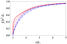
(a) metric function $f$

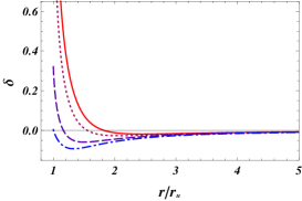
(b) lapse function $\delta$

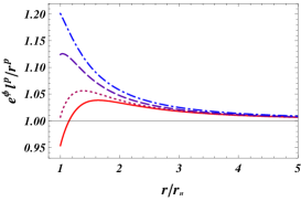
(c) dilaton field $\phi$

Figure 1: The metric functions $f$ and $\delta$ and the dilaton field $\phi$ in five dimensions for $k=-1$. We plot them normalized by the AdS values. We choose the following four values for the horizon radius: $r_{H}=$  0.70704304$\,\tilde{\alpha}_{2}^{1/2}$ (solid line), 0.70353475$\,\tilde{\alpha}_{2}^{1/2}$ (dotted line), 0.67226423$\,\tilde{\alpha}_{2}^{1/2}$ (dashed line), and 0.62013066$\,\tilde{\alpha}_{2}^{1/2}$ (dot-dashed line).

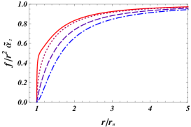
(a) metric function $f$

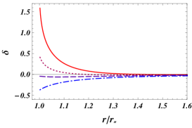
(b) lapse function $\delta$

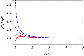
(c) dilaton field $\phi$

Figure 2: The metric functions $f$ and $\delta$ and the dilaton field $\phi$ in ten dimensions for $k=-1$. We plot them normalized by the AdS values. We choose the following four values for the horizon radius: $r_{H}=$  1.1486586$\,\tilde{\alpha}_{2}^{1/2}$ (solid line), 1.0894228$\,\tilde{\alpha}_{2}^{1/2}$ (dotted line), 0.9164287$\,\tilde{\alpha}_{2}^{1/2}$ (dashed line), and 0.7976378$\,\tilde{\alpha}_{2}^{1/2}$ (dot-dashed line).

The metric function monotonically approaches the asymptotic value in both five and ten dimensions. In five dimensions the lapse function decreases near the horizon and increasingly gets close to the asymptotic value, while in ten dimensions it monotonically gets close to the asymptotic value.

The range for the horizon radius of AdS black hole solutions is summarized in Table 5. No regular asymptotically AdS black hole solution is found in four dimensions.

In five dimensions, there is no lower bound but exists the upper bound, i.e., $0<r_{H}\leq 0.707087\,\tilde{\alpha}_{2}^{1/2}$. Note that there is no regular solution without a horizon ($r_{H}=0$). In dimensions higher than five, we find both lower and upper bounds. For example, in six and ten dimensions, we find $0.514410\,\tilde{\alpha}_{2}^{1/2}\leq r_{H}\leq 0.894427\,\tilde{\alpha}_{2}^{1/2}$ and $0.782926\,\tilde{\alpha}_{2}^{1/2}\leq r_{H}\leq 1.154671\,\tilde{\alpha}_{2}^{1/2}$, respectively. The maximum bound on the horizon radius is given by $r_{H}=\sqrt{2(D-4)/(D-1)}\,\tilde{\alpha}_{2}^{1/2}$ in (51), at which the quadratic term in the condition (44) for a regular horizon vanishes.

Comparing Table 5 with Table 2, we find that the branches with larger horizon radii in Table 2 do not give an asymptotically AdS black hole solution, but only the smaller branches do.

Table 5: The range of the horizon radius in which asymptotically AdS black holes exist for $k=-1$.

$D$	The range of horizon radius
4	${\rm None}$
5	$0.000000<r_{H}/\tilde{\alpha}_{2}^{1/2}\leq 0.707087$
6	$0.514410\leq r_{H}/\tilde{\alpha}_{2}^{1/2}\leq 0.894427$
7	$0.636016\leq r_{H}/\tilde{\alpha}_{2}^{1/2}\leq 0.999969$
8	$0.705191\leq r_{H}/\tilde{\alpha}_{2}^{1/2}\leq 1.069014$
9	$0.750436\leq r_{H}/\tilde{\alpha}_{2}^{1/2}\leq 1.118003$
10	$0.782926\leq r_{H}/\tilde{\alpha}_{2}^{1/2}\leq 1.154671$

The results obtained here show a sharp difference from the case of EDEGB without a cosmological constant, where no AdS black hole solutions are obtained for the asymptotic constant dilaton ohta_torii4 . The difference comes from the nontrivial dilaton field we consider here.

This solution is a dilatonic analogue of the non-general relativity branch or “AdS branch” of the black hole solution in the nondilatonic EGB theory; the asymptotically AdS black hole solution in the nondilatonic theory BH_EGB is given by

$$f(r):=k+\frac{(D-2)r^{2}}{2(D-4)\tilde{\alpha}_{2}}\left(1+\sqrt{1+\frac{8(D-4)\tilde{\alpha}_{2}\mu}{(D-2)r^{D-1}}}\right),$$

$$\delta(r)=0\,.$$ (70)

The asymptotic behaviour or the weak coupling limit, i.e., $\tilde{\alpha}_{2}\mu/r^{D-1}\ll 1$ of this solution (70), takes the form

$$f(r) \rightarrow k-\left[\frac{2\kappa_{D}^{2}}{(D-2)A_{D-2}}\right]\frac{M}{r^{D-3}}+\frac{(D-2)r^{2}}{(D-4)\tilde{\alpha}_{2}},$$ (71)

where we have introduced the area of $N$-dimensional unit sphere $A_{N}$ and gravitational mass $M$ as

$$A_{N} =2\pi^{(N+1)/2}/\Gamma[(N+1)/2],$$ (72)

$$M =-\frac{(D-2)A_{D-2}}{\kappa_{D}^{2}}\mu.$$ (73)

The asymptotic form (71) is the one for an AdS Schwarzschild solution with a negative mass, and it properly describes a black hole solution when it satisfies $f^{\prime}(r_{H})>0$ for $f(r_{H})=0$. This condition is satisfied for $k=-1$ and $r_{H}$ in the range

$$\frac{(D-4)(D-5)}{(D-2)(D-3)}\,\tilde{\alpha}_{2}\leq r_{H}^{2}\leq\frac{2(D-4)}{(D-2)}\,\tilde{\alpha}_{2}\,.$$ (74)

The upper bound (51) of the horizon radius for the dilatonic solution is smaller than that in the above inequality (74) for nondilatonic case. In fact, we find that the allowed range of horizon radius of our present black holes is always included in that in the EGB model, comparing Table 5 with (74).

V.2 Thermodynamical properties of numerical solution

Next we present the thermodynamical variables of the AdS black holes. We can define the temperature of black holes as a period of Euclidean time coordinate at event horizon

$$T_{H}=\frac{1}{4\pi}f^{\prime}_{H}e^{-\delta_{H}},$$ (75)

where $f^{\prime}_{H}$ and $\delta_{H}$ are determined by fixing the horizon radius $r_{H}$. For the asymptotically AdS solution in EGB (70), the temperature is explicitly given by

$$T_{H\rm{(EGB)}}=\frac{\left[(D-2)_{3}r_{H}^{2}-(D-4)_{5}\tilde{\alpha}_{2}\right]}{4\pi r_{H}\left[(D-2)r_{H}^{2}-2(D-4)\tilde{\alpha}_{2}\right]}\,.$$ (76)

Since we consider the higher-curvature correction terms, we apply Wald’s formula for a black hole entropy, which is generalization of the Bekenstein-Hawking formula to the case of most generic covariant theory. Wald’s formula is defined by use of the Noether charge associated with diffeomorphism invariance of a system Wald_formula . We find

$$S=-2\pi\int_{\Sigma}\frac{\partial{\cal L}}{\partial R_{{\mu\nu}\rho\sigma}}\epsilon_{{\mu\nu}}\epsilon_{\rho\sigma},$$ (77)

where $\Sigma$ is the $(D-2)$-dimensional surface of the event horizon, ${\cal L}$ is the Lagrangian density, and $\epsilon_{\mu\nu}$ denotes the volume element binormal to $\Sigma$. Although it was originally proposed for asymptotically flat spacetime, we assume that it is applicable in the present system. In Dutta , it is confirmed that Wald’s formula for asymptotically AdS black hole solutions is still valid for gravity theories with higher-curvature corrections, by comparing the result with the one obtained by the Euclidean regularization method. For the effective action in the string frame, it gives

$$S =\frac{e^{-2\phi_{H}}A_{H}}{4}\left(1+\frac{2\tilde{\alpha}_{2}}{r_{H}^{2}}\right),$$ (78)

where $A_{H}=A_{D-2}r_{H}^{D-2}$ is the area of the event horizon. The entropy for the EGB gravity is given by

$$S_{\rm(EGB)} =\frac{A_{H}}{4}\left(1+\frac{2\tilde{\alpha}_{2}}{r_{H}^{2}}\right).$$ (79)

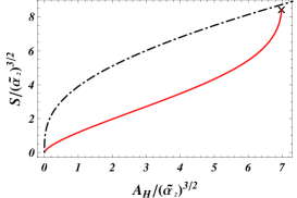
(a) $A_{H}$-$S$ relation in five dimensions

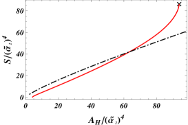
(b) $A_{H}$-$S$ relation in ten dimensions

Figure 3: The relations between the horizon area and entropy (a) in five dimensions and (b) in ten dimensions for $k=-1$. The solid line in red and the dashed line in black correspond to the cases of the DEGB and EGB gravity theories, respectively. The maximum horizon area in five dimensions is given by $A_{H,\rm{max}}=6.9782851\,\tilde{\alpha}_{2}^{3/2}$ denoted by $\times$, which corresponds to $r_{H}=0.70708722\,\tilde{\alpha}_{2}^{1/2}$. In ten dimensions the range of the horizon area of the obtained numerical black hole solutions is given by $4.1913928\,\tilde{\alpha}_{2}^{4}<A_{H}<93.8048858\,\tilde{\alpha}_{2}^{4}$, which corresponds to the range of horizon radii as $0.78293332\,\tilde{\alpha}_{2}^{1/2}<r_{H}<1.1546707\,\tilde{\alpha}_{2}^{1/2}$.

We depict the area-entropy relation in five and ten dimensions in Fig. 3. Since we have the Gauss-Bonnet higher-curvature term, the entropy is not proportional to the area; i.e., the Bekenstein-Hawking entropy formula is modified, but it still increases monotonically as the horizon area increases. We also plot the relation for the black holes in the EGB gravity theory as a reference. In any dimensions, the entropy increases as the horizon gets large. The entropy approaches zero as the horizon approaches the smallest size, which is zero for five dimensions and a finite size for other dimensions. Around the largest horizon limit, the derivative of the entropy seems to blow up to infinity. Since the entropy is smaller than that of EGB model in the small horizon region, the entropy curve for the obtained numerical solution crosses that for the EGB gravity in dimensions higher than five. In five dimensions, it seems to reach numerically the lowest bound before crossing.

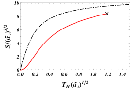
(a) $T_{H}$-$S$ relation in five dimensions

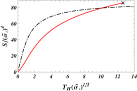
(b) $T_{H}$-$S$ relation in ten dimensions

Figure 4: The relations between the temperature and entropy (a) in five dimensions and (b) in ten dimensions for $k=-1$. The solid line in red and the dot-dashed line in black correspond to the cases of the DEGB and EGB models, respectively. The maximum temperature is given by $T_{H,\rm{max}}=1.18263054\,\tilde{\alpha}_{2}^{1/2}$ in five dimensions, while $T_{H,\rm{max}}=12.6217055\,\tilde{\alpha}_{2}^{1/2}$ in ten dimensions. Those end points are denoted by $\times$. The temperature in the AdS branch of the EGB model has no bound in any dimensions.

We also depict the temperature-entropy relation in Fig. 4. The temperature of the black hole vanishes as horizon area approaches the minimum size in any dimension, while it diverges as the horizon area approaches the maximum size. This is similar to the case of the EGB gravity model.

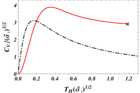
(a) $T_{H}$-$C_{V}$ relation in five dimensions

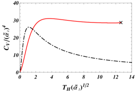
(b) $T_{H}$-$C_{V}$ relation in ten dimensions

Figure 5: The relations between specific heat and temperature (a) in five dimensions and (b) in ten dimensions for $k=-1$. The solid line in red and the dot-dashed line in black correspond to the cases of the DEGB and EGB models, respectively. The maximum-temperature points are denoted by $\times$.

The specific heat $C_{V}$ of a black hole solution is given by

$$C_{V}=T\left(\frac{\partial S}{\partial T}\right)_{V}.$$ (80)

We show the relation between the specific heat and the temperature in Fig. 5. The specific heat is positive for our solutions similar to that of AdS black hole in the EGB model Neupane . In the nondilatonic EGB gravity, the specific heat is negative for the $k=1$ black hole including the Schwarzschild solution, while it is positive for $k=-1$ BH_EGB ; AdSBH_EGB . Since the specific heat is always positive for our solution as shown in Fig. 5, we do not expect the Hawking-Page transition.

In order to discuss black hole thermodynamics, we have to find a mass and a scalar charge of a black hole. To extract the terms of a “mass” and a “scalar charge”, we introduce the following variables as

$$m[r] \equiv r^{D-3-2p}\left(f[r]-\bar{f}[r]\right)$$ (81)

$$\rightarrow\mu_{f}~{}~{}~{}{\rm as}~{}~{}~{}r\rightarrow\infty,$$

$$\Phi[r] \equiv r^{D-1-2p}\left(\phi[r]-\bar{\phi}[r]\right)$$ (82)

$$\rightarrow\mu_{\phi}~{}~{}~{}{\rm as}~{}~{}~{}r\rightarrow\infty\,.$$

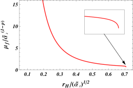
(a) ”mass” in five dimensions

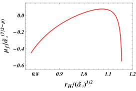
(b) ”mass” in ten dimensions

Figure 6: “Mass” $\mu_{f}$ in terms of the horizon radius for $k=-1$.

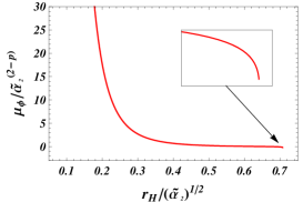
(a) “scalar charge” in five dimensions

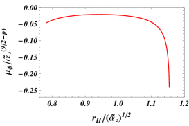
(b) “scalar charge” in ten dimensions

Figure 7: The “scalar charge” $\mu_{\phi}$ in terms of the horizon radius for $k=-1$.

In Figs. 6 and 7, we depict “mass” and “scalar charge” defined by (81) and (82), respectively. The solutions are classified into two categories; (a) odd dimensions and (b) even dimensions, according to their behaviour of the “mass” and “scalar charge”. In odd dimensions the “mass” monotonically decreases as the horizon radius increases and approaches zero in the upper limit of the horizon radius. On the other hand, the “mass” in even dimensions is not a monotonic function; i.e., as the horizon radius increases, it first increases and then decreases just after it reaches the maximum “mass”. It is not even positive. The “scalar charge” behaves similarly to the “mass” function in both odd and even dimensions. However, the present “mass” and “scalar charge” are not the physical ones. Hence we cannot discuss thermodynamics of our black holes furthermore.

These odd behaviours of the “mass” and “scalar charge” may be related to the fact that the AdS (or asymptotically AdS) spacetime of our system is realized not by a negative cosmological constant but by a dilaton field which diverges logarithmically at infinity. This type of solution does not exist if we assume that a dilaton field is finite, which is also true for the EDEGB case ohta_torii2 .

VI Summary and Conclusion

In the DEGB gravity, we have obtained the exact AdS spacetimes with a planar symmetry and constructed the asymptotically AdS black holes numerically. These solutions are the dilatonic generalization of AdS spacetime and the AdS branch of black hole solutions in the EGB gravity. A dilaton field, which diverges logarithmically at infinity, plays the role of a negative cosmological constant.

The allowed horizon radii for asymptotically AdS black holes seem to be inherited from those of the corresponding solutions in the AdS branch in the EGB gravity.

As for the thermodynamical properties of the black holes, the entropy and temperature are well defined and their behaviours are similar to those of the “AdS branch” solution with a hyperbolic horizon in the EGB gravity. However, we could not define the proper mass and charge, although we have introduced a “mass” term and “scalar charge”, which may carry some physical properties of the black holes. It makes it difficult for us to continue our discussion on thermodynamics such as the first law further. This strange behaviour of “mass” and “charge” may come from the fact that a dilaton field diverges logarithmically at infinity.

We hope that AdS spacetimes and the asymptotically AdS black holes obtained here give insight into the the AdS/CFT correspondence and reveal aspects of strong coupling physics such as those studied in Cai1 . In Appendix A, we show that AdS spacetime is also a solution for the models with more corrections in the string theory. Examining the CFT duals of AdS spacetimes we obtained in Sec. II and Appendix A would be an interesting issue.

Appendix A AdS spacetime in dilatonic Lovelock gravity

In this appendix, we extend our AdS solution for $k=0$ in the DEGB theory to the $D$-dimensional Lovelock gravity coupled to a dilaton field, whose action in the string frame is given by

$$S_{\!S}=\frac{1}{2\kappa_{D}^{2}}\int d^{D}\!x\sqrt{-g}\ e^{-2\phi}\,\biggl{(}R[g]+4{\nabla}_{\mu}\phi{\nabla}^{\mu}\phi+\sum^{[D/2]}_{n=2}\alpha_{n}E_{2n}[g]\biggr{)},$$ (83)

where $\alpha_{n}$ is the $n$th order coupling constant and the $n$th order Euler density $E_{2n}[g]$ is defined by

$$E_{2n}[g]=\frac{-1}{2^{n}\,(D-2n)!}R^{\mu_{1}\nu_{1}}\!_{\rho_{1}\sigma_{1}}[g]\cdots R^{\mu_{n}\nu_{n}}\!_{\rho_{n}\sigma_{n}}[g]\,\epsilon^{\alpha_{1}\alpha_{2}\cdots\alpha_{D-2n}\rho_{1}\sigma_{1}\cdots\rho_{n}\sigma_{n}}\epsilon_{\alpha_{1}\alpha_{2}\cdots\alpha_{D-2n}\mu_{1}\nu_{1}\cdots\mu_{n}\nu_{n}}.$$

This special combination of curvatures guarantees that $E_{2n}[g]$ is totally divergent in a $2n$-dimensional space, and its integration gives just a topological invariant. For $n=2$, it is known as the Gauss-Bonnet curvature term, which we have analyzed in the text.

In order to find an AdS spacetime, we adopt the same metric ansatz as in Sec. II. The explicit form of the action with this ansatz is given by

$$S_{\!S}=\frac{1}{2\kappa_{D}^{2}}\int d^{D}\!xe^{{W}-2\phi}\biggl{[} e^{-2\lambda}\bigl{(}2(D-2){Y}+(D-2)_{3}{A}-4\phi^{\prime}\nu^{\prime}\bigr{)}\biggr{.}+4e^{-2\lambda}\phi^{\prime 2}$$

$$+ \sum^{[D/2]}_{n=2}\tilde{\alpha}_{n}e^{-2n\lambda}\bigl{(}(D-2n)_{2n+1}{A}^{n}+2n(D-2n){Y}{A}^{n-1}-4n\phi^{\prime}\nu^{\prime}{A}^{n-1}\bigr{)}\biggl{.}\biggr{]},$$ (84)

where we have dropped surface terms and used a normalized coupling constant $\tilde{\alpha}_{n}\equiv(D-2)_{2n-1}\alpha_{n}$. The metric components $\lambda,\mu,$ and $\nu$ are defined by the metric ansatz (3), and $W,Y,$ and $A$ are given by Eq. (II). Taking the variation of this action with respect to $\nu$, $\lambda$, $\mu$, and $\phi$, we find four basic equations:

$$F_{{\rm(L)}\phi}:= -2\Bigl{\{}(D-2)_{3}A+2(D-2)(Y+Z)+2X+4\bigl{[}\left(\nu^{\prime}-\lambda^{\prime}+(D-2)\mu^{\prime}-\phi^{\prime}\right)\phi^{\prime}+\phi^{\prime\prime}\bigr{]}$$

$$+ \sum_{n}^{[D/2]}\tilde{\alpha}_{n}e^{-2n\lambda}\Bigl{[}(D-2n)_{2n+1}A^{n}+2n(D-2n)(Y+Z)A^{n-1}+2nXA^{n-1}+4n_{1}YZA^{n-2}\Bigr{]}\Bigr{\}}=0,$$ (85)

$$F_{{\rm(L)}\nu}:= (D-2)_{3}A+2(D-2)(Y+2\phi^{\prime}\mu^{\prime})+4(\phi^{\prime\prime}-\phi^{\prime 2}-\phi^{\prime}\lambda^{\prime})$$

$$+ \sum_{n}^{[D/2]}\tilde{\alpha}_{n}e^{-2n\lambda}\Bigl{[}(D-2n)_{2n+1}A^{n}+2n(D-2n)\left(Y+2\phi^{\prime}\mu^{\prime}\right)A^{n-1}$$

$$\hskip 56.9055pt+4n\left(\phi_{n}^{\prime\prime}-2\phi^{\prime 2}\right)A^{n-1}-4n\phi^{\prime}\lambda^{\prime}A^{n-1}+8n_{1}\phi^{\prime}\mu^{\prime}YA^{n-2}\Bigr{]}=0,~{}~{}~{}~{}~{}~{}~{}~{}~{}~{}~{}~{}~{}~{}~{}~{}~{}~{}~{}~{}~{}~{}~{}~{}~{}~{}~{}~{}~{}~{}~{}~{}~{}~{}~{}$$ (86)

$$F_{{\rm(L)}\lambda}:= (D-2)_{3}A+2(D-2)(Z+2\phi^{\prime}\mu^{\prime})+4(\nu^{\prime}-\phi^{\prime})\phi^{\prime}$$

$$+ \sum_{n}^{[D/2]}\tilde{\alpha}_{n}e^{-2n\lambda}\Bigl{[}(D-2n)_{2n+1}A^{n}+2n(D-2n)\left(Z+2\phi^{\prime}\mu^{\prime}\right)A^{n-1}+4n\phi^{\prime}\nu^{\prime}A^{n-1}+8n_{1}\phi^{\prime}\mu^{\prime}ZA^{n-2}\Bigr{]}=0,$$ (87)

$$F_{{\rm(L)}\mu}:= (D-2)_{4}A+2(D-2)_{3}(Y+Z+2\phi^{\prime}\mu^{\prime})+2(D-2)X+4(D-2)\left(\phi^{\prime\prime}-\phi^{\prime 2}+\phi^{\prime}\nu^{\prime}-\phi^{\prime}\lambda^{\prime}\right)$$

$$+ \sum_{n}^{[D/2]}\tilde{\alpha}_{n}e^{-2n\lambda}\Bigl{[}(D-2n)_{2n+2}A^{n}+2n(D-2n)_{2n+1}(Y+Z+2\phi^{\prime}\mu^{\prime})A^{n-1}+4n(D-2n)(\phi^{\prime\prime}-2\phi^{\prime 2})A^{n-1}$$

$$\hskip 48.36967pt+2n(D-2n)XA^{n-1}+4n(D-2n)(\nu^{\prime}-\lambda^{\prime})\phi^{\prime}A^{n-1}+8n_{1}(D-2n)(Y+Z)\phi^{\prime}\mu^{\prime}A^{n-2}$$

$$\hskip 48.36967pt+4n_{1}(D-2n)YZA^{n-2}+8n_{1}\left(\phi^{\prime\prime}-2\phi^{\prime 2}\right)ZA^{n-2}$$

$$\hskip 48.36967pt+8n_{1}\left(\mu^{\prime}X+\nu^{\prime}Y-\lambda^{\prime}Z\right)\phi^{\prime}A^{n-2}+16n_{2}\phi^{\prime}\mu^{\prime}YZA^{n-3}\Bigr{]}=0,$$ (88)

where we have introduced

$${X}=-\left(\nu^{\prime\prime}+\nu^{\prime 2}-\lambda^{\prime}\nu^{\prime}\right)\,,~{}{Z}=-\mu^{\prime}\nu^{\prime}\,,$$ (89)

in addition to (II). The Bianchi identity is also satisfied. Hence we have to solve three equations as in Sec. II.

In order to obtain an exact AdS spacetime, we take the same ansatz (16) and (17) as in Sec. II. We then find the following three algebraic equations:

$$\left[D_{1}-4p(D-1)+4p^{2}\right]+D_{1}{\rm S}_{1}=0\,,$$ (90)

$$p+p(1+2p){\rm S}_{2}=0\,,$$ (91)

$$L\left[(D-1)_{2}-4p(D-2)+4p^{2}\right]+{\rm S}_{3}=0\,,~{}~{}~{}$$ (92)

where $L\equiv-1/\ell^{2}$ and

$${\rm S}_{1} =\!\sum_{n=2}^{[D/2]}\!\tilde{\alpha}_{n}L^{n-1}\,,$$

$${\rm S}_{2} =\!\sum_{n=2}^{[D/2]}\!\tilde{\alpha}_{n}L^{n-1}n\,,$$ (93)

$${\rm S}_{3} =\!\sum_{n=2}^{[D/2]}\!\tilde{\alpha}_{n}L^{n}\!\left[(D-1)(D-2n)-4np(D-2)+8np^{2}\right],$$

Equation (90) with Eq. (91) gives Eq. (92). It means that three algebraic equations are not independent. Hence we have to solve the following two algebraic equations: (90) and (91) for two variables ($\varpi=1+2p$ and $L=-1/\ell^{2}$), i.e.,

$$1+\varpi~{}{\rm S}_{2}=0,$$ (94)

$$\varpi^{2}-2D\varpi+(D^{2}+D-1)+D_{1}~{}{\rm S}_{1}=0.$$ (95)

Eliminating $\varpi$, we obtain

$$F(L)\equiv{\rm S}_{2}^{2}\left(D^{2}+D-1+D_{1}~{}{\rm S}_{1}\right)-2D~{}{\rm S}_{2}+1=0.$$ (96)

$F(L)$ is the $3(n_{\rm max}-1)$th order algebraic equation with respect to $L$, where $n_{\rm max}$ is the highest order with nontrivial $\tilde{\alpha}_{n}$ ($n_{\rm max}\leq[D/2]$). If $n_{\rm max}$ is even , i.e., $3(n_{\rm max}-1)$ is odd, we always find a negative solution ($L<0$) for Eq. (96), since $F(0)=1>0$, that is, an AdS space. On the other hand, if $n_{\rm max}$ is odd, the existence of AdS space is no longer guaranteed.

If we have only one Lovelock term, for example, the $n_{0}$th Lovelock term $(n_{0}\leq[D/2])$, we can conclude more concretely

$$1+\varpi\tilde{\alpha}_{n_{0}}L^{{n_{0}}-1}n_{0}=0\,,$$ (97)

$$\varpi^{2}-2D\varpi+D^{2}+D-1+\tilde{\alpha}_{n_{0}}L^{{n_{0}}-1}=0\,.~{}~{}~{}~{}~{}~{}~{}~{}~{}~{}$$ (98)

Eliminating the terms with $L^{{n_{0}}-1}$, we obtain the third-order algebraic equation for $\varpi$:

$$\varpi^{3}-2D\varpi^{2}+(D^{2}+D-1)\varpi-\frac{D(D-1)}{n_{0}}=0\,,$$

(99)

which has always a positive real root $\varpi_{0}(>0)$. From (97) we find

$$L_{*}^{n_{0}-1}=-\frac{1}{n_{0}\tilde{\alpha}_{n_{0}}\varpi_{0}}\,.$$ (100)

Since $\tilde{\alpha}_{n_{0}}>0$, we find a solution with $L_{*}<0$ if $n_{0}$ is even but no solution for odd $n_{0}$.

In the string theory, we expect only even $n$’s. Hence we always find at least one AdS solution. For example, we consider the case of the heterotic string model such as ($D=10$, $\alpha_{2}=\alpha^{\prime}/8$, $\alpha_{3}=0$ and $\alpha_{4}=\alpha^{\prime 3}/8$). Then we find

$$p=-0.36469898\,,~{}\ell=3.91866401\alpha^{\prime 1/2}\,.$$ (101)

Appendix B “Solitonic” solution with AdS boundary

We also find a solitonic solution without a horizon but with a regular center, which approaches asymptotically an AdS spacetime. In this appendix, we leave the global topology $k$ free at first and fix it later. To solve the basic equations under a regularity condition at the origin ($r=0$), we expand the variables around the origin $r=0$ as

$$f(r) = \hat{f}_{0}+\hat{f}_{1}r+\hat{f}_{2}r^{2}+{\cal O}(r^{3})~{},$$

$$\delta(r) = \hat{\delta}_{0}+\hat{\delta}_{1}r+\hat{\delta}_{2}r^{2}+{\cal O}(r^{3})~{},$$ (102)

$$\phi(r) = \hat{\phi}_{0}+\hat{\phi}_{1}r+\hat{\phi}_{2}r^{2}+{\cal O}(r^{3})~{}.$$

The shift symmetry of $\phi$ and $\delta$ allows us to choose $\hat{\delta}_{0}=\hat{\phi}_{0}=0$. Substituting (102) into the field equations, we find that $\hat{f}_{0}=k$ in the leading equations and $\hat{f}_{1}=\hat{\delta}_{1}=\hat{\phi}_{1}=0$ in the second leading ones. The third leading equations give

$$D(\hat{f}_{2}-1)\hat{f}_{2}+4k(1-2\hat{f}_{2})\hat{\delta}_{2}+8k\hat{\phi}_{2}=0~{},$$

$$D(\hat{f}_{2}-1)\hat{f}_{2}+2(1-2\hat{f}_{2})(\hat{f}_{2}+4k\hat{\phi}_{2})=0~{},$$ (103)

$$(1-2\hat{f}_{2})(2\hat{\phi}_{2}-(D-2)\hat{\delta}_{2})-4\hat{\delta}_{2}(\hat{f}_{2}+4k\hat{\phi}_{2})=0~{}.$$

We show the numerical solutions of (103) in Table 6.

Table 6: The solutions for Eq. (103) for $k=1$ which give an asymptotically AdS spacetime.

$D$	$\hat{f}_{2}$	$\hat{\delta}_{2}$	$\hat{\phi}_{2}$
4	$1.0850432$	$-0.31739860$	$-0.23182971$
5	$1.1231984$	$-0.20045991$	$-0.21141146$
6	$1.1298841$	$-0.13500237$	$-0.19510138$
7	$1.1241759$	$-0.097812087$	$-0.18319807$
8	$1.1150320$	$-0.075149215$	$-0.17448348$
9	$1.1056361$	$-0.060330293$	$-0.16793263$
10	$1.0969813$	$-0.050055266$	$-0.16286547$

Adopting (102) with the solutions of (103) as the boundary conditions at the origin, we numerically solve the field equations. Note that we have no free parameter at the origin. We find two branches of solutions for $k=1$: One approaches asymptotically an AdS spacetime, and the other evolves into a singularity. We depict our numerical solution in Fig. 8.

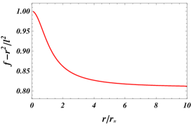
(a) $f(r)-r^{2}/\ell^{2}$
                                   
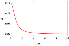
(b) $\delta(r)$
                                   
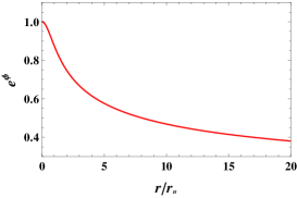
(c) $e^{\phi(r)}$

Figure 8: The solitonic AdS solution in five dimensions for $k=1$. We depict the configurations of $[f(r)-r^{2}/\ell^{2}]$, $\delta(r)$, and $e^{\phi(r)}$.

Analyzing the asymptotic behaviours, we find a similar result to the AdS black hole with $k=-1$ discussed in Sec. IV.2. Just as the black hole solutions, we present the “mass” and “scalar charge” in Table 7, which depend only on the spacetime dimensions $D$ and the coupling constant $\alpha_{2}$. No additional free parameter appears.

For $k=-1$, for which we obtain the AdS black hole, we could not obtain a regular solution but always find a singularity at a finite radius. For $k=0$, we obtain the exact AdS spacetime studied in Sec. II.

Table 7: “Mass” and the “scalar charge” introduced in (81) and (82) for $k=1$.

$D$	$\mu_{f}$	$\mu_{\phi}$
4	$-0.64077734$	$-0.056993109$
5	$0.17163694$	$0.016651835$
6	$0.13056579$	$0.013608420$
7	$-0.067443667$	$-0.0074559764$
8	$-0.061032657$	$-0.0070525786$
9	$0.039077656$	$0.0046311897$
10	$0.037257968$	$0.0045987537$

Appendix C Cosmological solution

For $k=-1$, we also find a cosmological solution instead of an AdS black hole. When we integrate the basic equations with the boundary conditions for a regular horizon, we find that the metric function $F$ is always negative in the larger-radius branch in Table 2. It means that the “time” coordinate $t$ plays no longer a role of time. Instead, the “radial” coordinate $r$ becomes time. Hence we exchange the characters of two coordinates as $\eta:=r$ and $\xi:=t$. The line element is given by

$$ds^{2}=-f_{C}^{-1}(\eta)d\eta^{2}+f_{C}(\eta)e^{-2\delta(\eta)}d\xi^{2}+\eta^{2}d\Sigma_{-1}^{2}\,,$$

where $f_{C}(\eta)=-f(r)$. The asymptotic behaviour of the metric functions and the dilaton field is given by

$$f_{C}[\eta] =\left[1-\left(\frac{\eta_{\infty}}{\eta}\right)^{D-3}\right]+{\cal O}\left(\frac{1}{\eta^{D-3}}\right)$$ (104)

$$\delta[\eta] ={\cal O}\left(\frac{1}{\eta^{2(D-3)}}\right)$$ (105)

$$\phi[\eta] =\phi_{\infty}+{\cal O}\left(\frac{1}{\eta^{2(D-3)}}\right)$$ (106)

as $\eta\rightarrow\infty$, where $\eta_{\infty}$ is a constant. Near the “horizon”, $f_{C}(\eta)$ vanishes as $f_{C}(\eta)\propto(\eta-\eta_{H})$, where $\eta_{H}:=r_{H}$ is the “horizon” radius.

We introduce a cosmic time $\tau$ by

$$\tau=\int_{\eta_{H}}^{\eta}d\eta\,f_{C}^{-1/2}(\eta)\ .$$ (107)

Using this cosmic time, we can rewrite the line element as

$$ds^{2}=-d\tau^{2}+a^{2}(\tau)d\Sigma_{-1}^{2}+b^{2}(\tau)d\xi^{2}\,,$$ (108)

where the metric functions $a(\tau)$ and $b(\tau)$ are defined by

$$a:=\eta(\tau)\,,~{}~{}b:=f_{C}^{1/2}e^{-\delta}\,,$$ (109)

and the asymptotic behaviours as $\tau\rightarrow\infty$ are

$$a\rightarrow\tau\left(1+\frac{\tau_{\infty}^{D-3}}{2(D-4)\tau^{D-3}}\right)\,,b\rightarrow 1-\frac{\tau_{\infty}^{D-3}}{2\tau^{D-3}}\,,~{}~{}$$ (110)

where $\tau_{\infty}:=\eta_{\infty}$. The asymptotic metric is given by

$$ds^{2}=-d\tau^{2}+\tau^{2}d\Sigma_{-1}^{2}+d\xi^{2}\,,$$ (111)

which is a [$(D-1)$-dimensional Milne universe] $\times{\bf R}^{1}$. See Milne for a Milne universe.

We depict numerical solutions in Fig. 9. It shows that the spacetime starts from a big bang singularity and evolves into the [$(D-1)$-dimensional Milne universe] $\times{\bf R}^{1}$. These solutions are obtained in the larger-radius branch of $r_{H}(=\eta_{H})$ in Table 2.

For $D=5$, we show our numerical result in Fig. 9. By compactifying the fifth direction ($\xi$), we find a four-dimensional bouncing universe. The three-dimensional space with the scale factor $a$ bounces at $\tau=0$ and evolves into a Milne universe. Although the fifth dimension with the scale factor $b$ starts from an initial big bang singularity, it eventually approaches a constant space as $\tau\rightarrow\infty$.

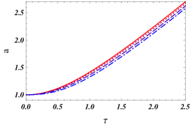
(a) $a(\tau)[=\eta(\tau)]$

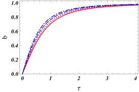
(b) $b(\tau)$

Figure 9: We depict two scale factors $a(\tau)[=\eta(\tau)]$ and $b(\tau)$ in five dimensions for $k=-1$. We choose the following four values for the “horizon radius”: $\eta_{H}=\,$31.6227766 $\tilde{\alpha}_{2}^{1/2}$ (solid line), 4.14479601  $\tilde{\alpha}_{2}^{1/2}$ (dotted line), 2.97463549 $\tilde{\alpha}_{2}^{1/2}$ (dashed line), and 2.62725036  $\tilde{\alpha}_{2}^{1/2}$ (dot-dashed line).

References

- (1) D. Lovelock, J. Math. Phys. 12, 498 (1971); 13, 874 (1972).
-
(2)
D. G. Boulware, and S. Deser,
Phys. Rev. Lett. 55, 2656 (1985);
J. T. Wheeler, Nucl. Phys. B 268, 737 (1986);
D. L. Wiltshire, Phys. Lett. B 169, 36 (1986). - (3) D. G. Boulware, and S. Deser, Phys. Lett. B 175, 409 (1986).
- (4) R. G. Cai, Phys. Rev. D 65, 084014 (2002) [arXiv:hep-th/0109133].
-
(5)
B. Zwiebach,
Phys. Lett. B 156, 315 (1985);
B. Zumino, Phys. Rep. 137, 109 (1986). - (6) R. R. Metsaev, and A. A. Tseytlin, Nucl. Phys. B 293, 385 (1987).
- (7) K. Maeda, N. Ohta, and Y. Sasagawa Phys. Rev. D 80, 104032 (2009) [arXiv:0908.4151[hep-th]].
- (8) P. Kanti, N. E. Mavromatos, J. Rizos, K. Tamvakis, and E. Winstanley, Phys. Rev. D 54, 5049 (1996) [arXiv:hep-th/9511071].
- (9) S. O. Alexeyev, and M. V. Pomazanov, Phys. Rev. D 55, 2110 (1997) [arXiv:hep-th/9605106].
- (10) T. Torii, H. Yajima, and K. Maeda, Phys. Rev. D 55, 739 (1997) [arXiv:gr-qc/9606034].
- (11) Z. K. Guo, N. Ohta, and T. Torii, Prog. Theor. Phys. 120, 581 (2008) [arXiv:0806.2481 [gr-qc]].
- (12) C. M. Chen, D. V. Gal’tsov, and D. G. Orlov Phys. Rev. D 75, 084030 (2007) [arXiv:hep-th/0701004]
- (13) C. M. Chen, D. V. Gal’tsov, and D. G. Orlov Phys. Rev. D 78, 104013 (2008) [arXiv:0809.1720[hep-th]]
- (14) C. M. Chen, D. V. Gal’tsov, N. Ohta, and D. G. Orlov Phys. Rev. D 81, 024002 (2010) [arXiv:0910.3488[hep-th]]
- (15) D. V. Gal’tsov, and E. A. Davydov, JETP Lett. 89, 102 (2009) [arXiv:0812.5103 [hep-th]].
- (16) M. Iihoshi [arXiv:1011.2088[hep-th]].
- (17) R. G. Cai, Z. Y. Nie, N. Ohta, and Y. W. Sun Phys. Rev. D 79, 066004 (2009) [arXiv:0901.1421[hep-th]].
- (18) S. W. Hawking, and D. N. Page Comm. Math. Phys. 87, 577 (1983).
- (19) D. Birmingham, Class. Quant. Grav. 16, 1197 (1999) [arXiv:hep-th/9808032 ].
- (20) I.P. Neupane, Phys. Rev. D 69, 084011 (2004) [arXiv:hep-th/0302132].
- (21) Z. K. Guo, N. Ohta, and T. Torii, Prog. Theor. Phys. 121, 253 (2009) [arXiv:0811.3068 [gr-qc]].
- (22) N. Ohta, and T. Torii, Prog. Theor. Phys. 121, 959 (2009) [arXiv:0902.4072 [hep-th]].
- (23) N. Ohta, and T. Torii, Prog. Theor. Phys. 122, 1477 (2010) [arXiv:0908.3918 [hep-th]].
- (24) N. Ohta, and T. Torii, Prog. Theor. Phys. 124, 207 (2010) arXiv:1004.2779 [hep-th].
- (25) V. Frolov, S. Hendy, and A. L. Larsen, Phys. Rev. D 54, 5093 (1996) [arXiv:hep-th/9510231].
- (26) R. G. Cai, and A. Wang, Phys. Rev. D 70, 084042 (2004) [arXiv:hep-th/0406040].
- (27) C. M. Chen, D. V. Gal’tsov, and N. Ohta, Phys. Rev. D 72, 044029 (2005) [arXiv:hep-th/0506216].
-
(28)
R. M. Wald,
Phys. Rev. D 48, R 3427 (1993)
[arXiv:gr-qc/9307038];
V. Iyer, and R. M. Wald, Phys. Rev. D 50, 846 (1994) [arXiv:gr-qc/9403028]. - (29) S. Dutta, and R. Gopakumar Phys. Rev. D 74, 044007 (2006) [arXiv:hep-th/0604070].
-
(30)
E. A. Milne,
Quart. J. Math. 5, 64 (1934);
W. H. McCrea, and E. A. Milne, Quart. J. Math. 5, 73 (1934).