SLAC–PUB–14320 December, 2010

Top Quark Amplitudes with an Anomalous Magnetic Moment

Andrew J. Larkoski and Michael E. Peskin

SLAC, Stanford University, Menlo Park, CA 94025 USA

ABSTRACT

The anomalous magnetic moment of the top quark may be measured during the first run of the LHC at 7 TeV. For these measurements, it will be useful to have available tree amplitudes with $t\overline{t}$ and arbitrarily many photons and gluons, including both QED and color anomalous magnetic moments. In this paper, we present a method for computing these amplitudes using the Britto-Cachazo-Feng-Witten (BCFW) recursion formula. Because we deal with an effective theory with higher-dimension couplings, there are roadblocks to a direct computation with the BCFW method. We evade these by using an auxiliary scalar theory to compute a subset of the amplitudes.

Submitted to Physical Review D

1 Introduction

The first run of the Large Hadron Collider (LHC) at 7 TeV promises to yield a wealth of data and could lead to hints at physics beyond the Standard Model. While we do not know what questions the LHC will answer in regards to electroweak symmetry breaking, supersymmetry, dark matter or other new physics, we can be sure that during the first run our knowledge of the Standard Model particles will increase. In particular, the number of top quarks that will be produced at the LHC will be comparable to that produced so far at the Fermilab Tevatron, and a much greater sample will be produced at large $t\overline{t}$ masses. This will give us an opportunity to probe for interactions of the top quark that might indicate its composite structure or coupling to new forces.

One aspect of this study will be the search for anomalous magnetic moment couplings of the top quark. The consequences of anomalous magnetic moments of the top quark have been considered previously, beginning with the work of Atwood, Kagan, and Rizzo [1] and Haberl, Nachtmann, and Wilch [2]. These authors analyzed top quark pair production; they computed the effect of the color anomalous magnetic moment on the total cross section and distributions of the top quarks for this process. At the high energies available at the LHC, however, one should also consider the effect of radiation of additional gluons. It would be useful to have a calculational method that could produce arbitrarily complicated tree amplitudes of this type.

In this paper, we will discuss a straightforward method for computing $t\overline{t}+ng+m\gamma$ tree amplitudes of arbitrary complexity. In principle, these amplitudes can be computed from Feynman diagrams. However, the multiple vertices and the complexity of gluon interactions make this a challenge. Already at the level of $t\overline{t}+4g$ processes, corresponding to $t\overline{t}$ production with 2 gluons radiated, there are over 100 Feynman diagrams. This number increases greater than factorially with the number of gluons. A better solution would be to compute the amplitudes recursively, using either the Berends-Giele approach [3] or the more recently proposed on-shell recursion formula of Britto, Cachazo, Feng, and Witten (BCFW) [4]. Some time ago, Schwinn and Weinzierl developed a formalism for massive quarks that uses the BCFW method and is computationally very effective for QCD tree amplitudes [5].

However, the Schwinn-Weinzierl scheme does not generalize directly to include the anomalous magnetic moment couplings. The BCFW method requires good behavior of amplitudes as some external momenta are taken to infinity. Thus it is nontrivial to apply this method to effective Lagrangians that involve higher-dimension interactions. Indeed, we find that direct application of the BCFW method is stymied by the additional momentum factor in the anomalous magnetic moment vertex.

Fortunately, there is a way around this difficulty. We find that those amplitudes that cannot be computed by direct application of BCFW can be computed using an auxiliary theory of a scalar particle that carries the spin internally. Combining the results, we produce a compact recursive method. This method introduces what we consider a promising approach to the application of on-shell recursion to general effective Lagrangians with higher-dimensional interactions.

The outline of this paper is as follows: In Section 2, we will present our notation and review some aspects of BCFW computation. In Section 3, we will analyze the use of BCFW recursion for fermions with anomalous magnetic moment couplings. In Section 4, we will present a useful rewriting of this theory as an auxiliary scalar theory. In Section 5, we will present some explicit calculations that check the relation of this scalar theory to the original fermion theory. In Section 6, we will present our conclusions and compare our approach to other work on the treatment of higher-dimension interactions by on-shell methods.

2 Review of Spinor Helicity and BCFW Recursion

The goal of this paper will be to present a method for tree-level calculations in the theory

$${\cal L}=\overline{\Psi}\biggl{[}i\not{\hbox{\kern-4.0pt$D$}}-m+{ga\over 4m}\Sigma_{\mu\nu}F^{\mu\nu a}t^{a}\biggr{]}\Psi\ ,$$ (1)

where $g$ is the QCD coupling, $a$ is a fixed constant color anomalous magnetic moment, $F^{\mu\nu a}$ is the QCD field strength, and $\Sigma_{\mu\nu}=i[\gamma_{\mu},\gamma_{\nu}]/2$. The same method will generalize readily if the theory also includes a QED anomalous magnetic moment term

$$\delta{\cal L}=+\overline{\Psi}\biggl{[}{2\over 3}{ea_{\mbox{\scriptsize QED}}\over 4m}\Sigma_{\mu\nu}F^{\mu\nu}\biggr{]}\Psi\ .$$ (2)

Throughout this paper, we will use the spinor helicity notation, as reviewed pedagogically in [6]. Instead of using 4-vectors, we will use as fundamental objects the spinor products

$$\langle ij\rangle=\overline{u}_{-}(i)u_{+}(j)\qquad[ij]=\overline{u}_{+}(i)u_{-}(j)\ .$$ (3)

associated with lightlike vectors $p_{i}$, $p_{j}$. These objects are antisymmetric and obey

$$|\langle ij\rangle|^{2}=|[ij]|^{2}=(p_{i}+p_{j})^{2}=s_{ij}\ .$$ (4)

The spinor completeness relation is written in this language as

$$p\rangle[p+p]\langle p=\not{\hbox{\kern-2.0pt$p$}}\ .$$ (5)

As an example, the polarization vectors of a gauge boson can be written as

$$\epsilon_{+}^{\mu}(k)={\langle r\gamma^{\mu}k]\over\sqrt{2}\langle rk\rangle}\qquad\epsilon_{-}^{\mu}(k)=-{[s\gamma^{\mu}i\rangle\over\sqrt{2}[sk]}\ ,$$ (6)

using auxiliary reference spinors $r$, $s$. The spinors $r$, $s$ are arbitrary, corresponding to the gauge freedom of the boson.

The spinor helicity formalism has been extended for use with massive fermions by Schwinn and Weinzierl (SW) [5]. For a massless fermion, the helicity states are physically distinct and Lorentz-invariant. For massive fermions, there is no unambiguous specification of spin state. In the formalism of SW, a lightlike reference vector $r$ is used to specify the spin basis to be used. Starting with the massive 4-vector $p$, one defines a lightlike 4-vector $p^{\flat}$ by

$$\not{\hbox{\kern-2.0pt$p$}}^{\flat}=p^{\flat}\rangle[p^{\flat}=\not{\hbox{\kern-2.0pt$p$}}-{m^{2}\over\langle rpr]}\not{\hbox{\kern-2.0pt$r$}}\ .$$ (7)

Then the $u_{+}(p)$, $u_{-}(p)$ spinors for a massive fermion are

$$u_{+}(p)={(p+m)r\rangle\over\langle p^{\flat}r\rangle}\qquad u_{-}(p)={(p+m)r]\over[p^{\flat}r]}\ .$$ (8)

It is straightforward to check that these spinors satisfy the required completeness relation.

We will express the values of fermion amplitudes by taking all fermions and antifermions to be outgoing. With this prescription, outgoing fermions are described by spinors $\overline{u}(p)$ given by

$$\mbox{for}\ q_{R}\ :\ {\langle r(p+m)\over\langle rp^{\flat}\rangle}\ ,\qquad\mbox{for}\ q_{L}\ :\ {[r(p+m)\over[rp^{\flat}]}\ ,$$ (9)

Outgoing antifermions are described by spinors $v(p)$ given by

$$\mbox{for}\ \overline{q}_{R}\ :\ {(p-m)r\rangle\over\langle p^{\flat}r\rangle}\ ,\qquad\mbox{for}\ \overline{q}_{L}\ :\ {(p-m)r]\over[p^{\flat}r]}\ .$$ (10)

To study the effects of top quark polarization, it is useful to be able to compute massive fermion amplitudes for an arbitrary choice of the reference vector $r$ for each fermion. We will try to retain that freedom in our analysis.

BCFW [4] proposed a method for computing QCD amplitudes based on the idea of deforming the external momenta by a complex parameter $z$ such that total momentum remains conserved and all particles remain on-shell. The explicit deformation they proposed chooses two particles $i$, $j$ and modifies their momenta according to

$$p_{i}\to p_{i}-zq\ ,\qquad p_{j}\to p_{j}+zq\ .$$ (11)

To keep particles $i$ and $j$ on-shell, $q$ must be light-like and satisfy $q\cdot p_{i}=q\cdot p_{j}=0$. For massless $i$ and $j$ this can be expressed as a deformation of the individual spinor components:

$$i\rangle\to i\rangle-z\>j\rangle\ ,\qquad i]\to i]\ ,$$

$$j\rangle\to j\rangle\ ,\qquad j]\to j]+z\>i]\ .$$ (12)

At tree level, the deformed amplitude ${\cal A}(z)$ has only simple poles in $z$ from Feynman propagators going on-shell. BCFW then considered the object

$$\oint{dz\over z}{\cal A}(z)\ ,$$ (13)

where the contour encircles $z=0$ and is taken to $\infty$. If ${\cal A}(z)\to 0$ as $z\to\infty$, the integral receives no contribution from the contour at $\infty$ and the integral vanishes. By Cauchy’s theorem, this is the sum of residues of poles in the contour. Then,

$${\cal A}(0)=-\sum\mbox{Res}\;{\cal A}(z)\ .$$ (14)

The quantity on the left-hand side of (14) is the original amplitude to be evaluated. The residues on the right occur when the deformed momentum that flows through a propagator goes on-shell. This relates lower point on-shell amplitudes to the amplitude of interest. BCFW thus obtain a recursion formula that allows the original amplitude ${\cal A}$ to be computed in terms of lower-point amplitudes.

More explicitly, the recursion relation is

$$i{\cal A}=\sum_{\mbox{\scriptsize cuts}}i{\cal A}_{\mbox{\scriptsize L}}(\hat{i})\ {i\over P_{\mbox{\scriptsize L}}^{2}}\ i{\cal A}_{\mbox{\scriptsize R}}(\hat{j})\ .$$ (15)

The sum runs over cuts through a single propagator that divide the amplitude into two parts, with the external leg $i$ in the left-hand amplitude ${\cal A}_{\mbox{\scriptsize L}}(\hat{i})$ and the external leg $j$ in the right-hand amplitude ${\cal A}_{\mbox{\scriptsize R}}(\hat{j})$. These amplitudes are computed with all momenta on-shell and with $i$ and $j$ set to their shifted values. The identity requires good large $z$ behavior of the amplitude ${\cal A}(z)$. If this amplitude does not tend to zero as $z\to\infty$, extra terms appear from the contour at $\infty$ that invalidate the simple recursion.

3 Large $z$ behavior

Since the BCFW recursion formula depends on good behavior of the shifted amplitude as $z\to\infty$, there is a danger that the BCFW method will not be valid for effective theories that contain non-renormalizable operators. In this section, we will show that this is a problem for the model (1). Specifically, we will show that tree amplitudes in the theory (1) can be computed in terms of amplitudes with all $+$ or $-$ gluon helicities. However, this still leaves a gap that needs to be filled before all amplitudes can be computed from simple components.

In our analysis of the theory (1), we will only consider shifts of gluon momenta. In [5], SW give a prescription for shifting the momenta of external massive fermions. However, this analysis works only for specific choices of the reference vector $r$ in (7), while we would like to maintain the freedom to work with an arbitrary choice of $r$.

An arbitrary shift on gluons will, according to (12), involve an external momentum $i$ with its angle bracket shifted and an external momentum $j$ with its square bracket shifted. There are four possible helicity combinations of the $ij$ to consider: $++$, $+-$, $--$ and $-+$. For standard QCD with $a=0$, the first three shifts give good $z\to\infty$ behavior while the last case $-+$ does not allow BCFW recursion. Still, for any two gluons, there is an allowed shift, and so any $q\overline{q}+ng$ amplitude can be reduced to 3-point functions by BCFW recursion.

Now consider adding to the theory the anomalous magnetic moment vertex. If the shift momentum $zq$ flows into the quark line through this vertex, the vertex is proportional to $z$ at large $z$. A fermion propagator carrying the shift momentum behaves as $z^{0}$, and all other fermion vertices—including the magnetic moment vertex with an ${\cal O}(1)$ external momentum—scale as $z^{0}$. If the gluon from the magnetic moment vertex is connected to external gluon lines through a tree of gluons, each propagator in this tree carrying the shift momentum scales as $z^{-1}$ and each vertex is at worst $z^{1}$. Then, finally, the worst possible behavior of amplitudes as $z\to\infty$ is $z^{2}$, times the $z$-dependence of the external gluon polarization vectors.

If we take $q$ as the reference vector for the polarization vectors of the shifted gluons, these polarization vectors scale as

$$\epsilon_{+}^{\mu}(\hat{i}) = {\langle q\gamma^{\mu}i]\over\sqrt{2}\langle q\hat{i}\rangle}\sim{1\over z}\ ,\qquad\epsilon_{+}^{\mu}(\hat{j})={\langle q\gamma^{\mu}\hat{j}]\over\sqrt{2}\langle qj\rangle}\sim z\ ,$$

$$\epsilon_{-}^{\mu}(\hat{i}) = -{[q\gamma^{\mu}\hat{i}\rangle\over\sqrt{2}[qi]}\sim z\ ,\qquad\epsilon_{-}^{\mu}(\hat{j})=-{[q\gamma^{\mu}j\rangle\over\sqrt{2}[q\hat{j}]}\sim{1\over z}\ .$$ (16)

We conclude that, in the three cases of shifts allowed in standard QCD, the shifted amplitudes behave at worst as

$\hat{i}$	$\hat{j}$	large $z$
$+$	$+$	$z^{2}$
$+$	$-$	$1$
$-$	$-$	$z^{2}$

However, the true situation is slightly better. For an anomalous magnetic moment vertex that stands in front of a fermion propagator carrying the shift momentum,

$$ga\Sigma^{\mu\nu}(zq_{\nu}+k_{\nu}){z\not{\hbox{\kern-2.0pt$q$}}+\not{\hbox{\kern-2.0pt$k$}}^{\prime}+m\over(zq+k^{\prime})^{2}-m^{2}}\ ,$$ (17)

we can rewrite

$$\Sigma^{\mu\nu}q_{\nu}=i(\gamma^{\mu}\not{\hbox{\kern-2.0pt$q$}}-q^{\mu})\ .$$ (18)

Since $q^{2}=(\not{\hbox{\kern-2.0pt$q$}})^{2}=0$, the $\not{\hbox{\kern-2.0pt$q$}}$ term cancels the leading term in the propagator, and the $q^{\mu}$ term either vanishes when dotted into a polarization vector or dots with a $q$ in a 3-gluon vertex and thus cancels the leading $z$ term in this vertex. For a magnetic moment vertex behind a fermion propagator carrying the shift momentum, a similar manipulation applies. This reduces the estimates in the table by at least a factor of $z^{-1}$. In this way, we see that the $+-$ shift allows a BCFW reduction, while the $++$ and $--$ shifts still may not.

To resolve these last cases, it is simplest to directly compute the amplitudes for 2 gluons with one magnetic moment vertex in the case of massless fermions. For massless fermions, (1) is not well-defined. However, a massless fermion can have an anomalous magnetic moment, and so we replace $m$ in the denominator of the last term in (1) with some high scale $M$. This prescription for massless fermions will also be used in the discussion in the Appendix. In standard QCD, the massless fermion amplitudes with two $+$ or $-$ helicity gluons vanish. With nonzero $a$, this is no longer the case. We find

$${\cal A}(q^{+},g_{1}^{+},g_{2}^{+},\overline{q}^{+})={g^{2}a\over 2M}{{[12]}^{2}\over\langle q\overline{q}\rangle}\ .$$ (19)

This expression behaves as $z^{0}$ after a $++$ shift on the gluons. In contrast

$${\cal A}(q^{-},g_{1}^{-},g_{2}^{+},\overline{q}^{-})=-{g^{2}a\over 2M}{{\langle q1\rangle}^{2}{\langle\overline{q}1\rangle}^{2}\over\langle q1\rangle\langle 12\rangle\langle 2\overline{q}\rangle}\ .$$ (20)

This behaves as $z^{-1}$ after a $+-$ shift. This confirms that our current estimates are, in general, the best possible. The BCFW recursion can be used to reduce amplitudes for which a $+-$ shift is possible, but, for $a\neq 0$, it cannot be used in the cases of $++$ and $--$ shifts.

Using $+-$ shifts only, we can reduce any amplitude for $q\overline{q}+ng$ to amplitudes that involve all $+$ helicity gluons or all $-$ helicity gluons. However, we cannot, in general, go further. We need another method to compute these cases, which are required as input to the general $q\overline{q}+ng$ amplitude.

For the case of gluons coupling to massless quarks, we have obtained an explicit formula for the amplitudes with all $+$ helicity gluons. This is presented in Appendix A. We have not succeeded in generalizing this to the case of massive fermions relevant for top quark physics. In the next section, we will take up another approach to this problem.

4 An Auxiliary Scalar Theory

We can make progress toward the computation of the all $+$ helicity gluon amplitudes by breaking up (1) into chiral components and rearranging it into a second-order Lagrangian.

Let $(\psi,\overline{\psi})$ be the left- and right-handed spinor components of $\Psi$, so that

$$\Psi=\pmatrix{\psi\cr\overline{\psi}\cr}\ ,\qquad\overline{\Psi}=\pmatrix{\overline{\psi}^{\dagger}&\psi^{\dagger}\cr}\ .$$ (21)

In this basis, the Dirac matrices take the form

$$\gamma^{\mu}=\pmatrix{0&\sigma^{\mu}\cr\overline{\sigma}^{\mu}&0\cr}$$ (22)

where $\sigma^{\mu}=(1,\vec{\sigma})^{\mu}$ and $\overline{\sigma}^{\mu}=(1,-\vec{\sigma})^{\mu}$, and

$$\Sigma^{\mu\nu}=2i\pmatrix{\sigma^{\mu\nu}&0\cr 0&\overline{\sigma}^{\mu\nu}\cr}\ ,$$ (23)

where

$$\sigma^{\mu\nu}={1\over 4}(\sigma^{\mu}\overline{\sigma}^{\nu}-\sigma^{\nu}\overline{\sigma}^{\mu})\quad\overline{\sigma}^{\mu\nu}={1\over 4}(\overline{\sigma}^{\mu}\sigma^{\nu}-\overline{\sigma}^{\nu}\sigma^{\mu})\ .$$ (24)

The Lagrangian (1) becomes

$${\cal L} = \psi^{\dagger}(i\overline{\sigma}\cdot D)\psi+\overline{\psi}^{\dagger}(i\sigma\cdot D)\overline{\psi}-m\psi^{\dagger}\overline{\psi}-m\overline{\psi}^{\dagger}\psi$$ (25)

$$\hskip 72.26999pt+i{ga\over 2m}\psi^{\dagger}(\overline{\sigma}_{\mu\nu}F^{\mu\nu a}t^{a})\overline{\psi}+i{ga\over 2m}\overline{\psi}^{\dagger}(\sigma_{\mu\nu}F^{\mu\nu a}t^{a})\psi\ .$$

Now formally integrate out $\overline{\psi}$ and $\psi^{\dagger}$. This gives

$${\cal L}=\overline{\psi}^{\dagger}\biggl{[}-m+i{ga\over 2m}\sigma_{\mu\nu}F^{\mu\nu a}t^{a}+\sigma\cdot D{1\over m-i(ga/2m)\overline{\sigma}_{\mu\nu}F^{\mu\nu a}t^{a}}\overline{\sigma}\cdot D\biggr{]}\psi\ .$$ (26)

After Taylor expanding the denominator and using the properties of the sigma matrices, this becomes

$${\cal L}={1\over m}\overline{\psi}^{\dagger}\biggl{[}-D^{2}-m^{2}-i{g\hat{g}_{L}\over 2}\sigma_{\mu\nu}F^{\mu\nu a}t^{a}-\sigma\cdot D\sum_{n=1}^{\infty}\biggl{(}{-iga\over 2m^{2}}\overline{\sigma}_{\mu\nu}F^{\mu\nu a}t^{a}\biggr{)}^{n}\overline{\sigma}\cdot D\biggr{]}\psi\ .$$ (27)

In this equation, the factor $a$ in front of $\sigma\cdot F$ in (26) has combined with a term arising from the commutator of covariant derivatives to produce the factor

$$\hat{g}_{L}=2+a$$ (28)

Thus, we obtain a second-order equation with a term close to the full magnetic moment of the fermion appearing explicitly. Note that (28) differs from the Landé $g$ factor of the fermion, which would be $(2+2a)$. The Landé $g$ factor refers to the behavior of the fermion in a background magnetic field. The $\vec{\sigma}\cdot\vec{B}$ term gets contributions both from $\sigma\cdot F$ and $\overline{\sigma}\cdot F$. Thus, the $n=1$ term in the sum in the last term also contributes to the Landé $g$ factor, supplying the missing contribution of $a$.

If we had chosen instead to integrate out $\psi$ and $\overline{\psi}^{\dagger}$, we would have obtained the same second-order action with the positions of $\sigma^{\mu\nu}$ and $\overline{\sigma}^{\mu\nu}$ interchanged. The significance of this exchange will be made clear below.

The procedure of integrating out components of the quark field is used in other contexts in infinite momentum frame quantization [7], light cone QCD [8], and soft and collinear effective field theory [9]. For the application here, we would like to emphasize that this integration out introduces no approximations. From (27), we are able to reconstruct any amplitude in the original theory. Although our new Lagrangian is not the most convenient way to obtain the scattering amplitudes in the limit $m\to 0$, it does give the correct answers in this limit, as we will illustrate in Section 5.

To analyze the consequences of (27), it is tempting to drop the series of terms with $\overline{\sigma}\cdot F$ and approximate this theory by

$${\cal L}={1\over m}\overline{\psi}^{\dagger}\biggl{[}-D^{2}-m^{2}+i{g\hat{g}_{L}\over 2}\sigma_{\mu\nu}F^{\mu\nu a}t^{a}\biggr{]}\psi\ .$$ (29)

This theory resembles a relativistic theory of a scalar field, except that this scalar retains a 2-component internal spin variable on which $\sigma^{\mu\nu}$ acts. In the following, we will refer to this model as a scalar theory even though it does describe spin $\frac{1}{2}$. To better understand the relation of this theory to the original Dirac theory, note that if we start from the Dirac equation with $a=0$

$$(i\not{\hbox{\kern-4.0pt$D$}}-m)\Psi=0$$ (30)

and multiply by $(i\not{\hbox{\kern-4.0pt$D$}}+m)$ on the left, we obtain

$$(-D^{2}-m^{2}+{g\over 2}\Sigma_{\mu\nu}F^{\mu\nu a}t^{a})\Psi=0\ ,$$ (31)

in which the top two components are precisely the equation of motion from (29) with $\hat{g}_{L}=2$. The equation (31) arises in calculating of the determinant of the Dirac operator, for example, in the background-field derivation of the QCD beta function.

In general, there is no justification for approximating (27) by (29). However, we are interested here in computing the amplitude for $q\overline{q}$ plus gluons with $+$ helicity only. A configuration of gluons with all $+$ helicities is a self-dual Yang-Mills field [10]. The operator $\sigma_{\mu\nu}F^{\mu\nu}$ projects onto self-dual field configurations. Conversely, $\overline{\sigma}_{\mu\nu}F^{\mu\nu}$ projects onto anti-self-dual configurations and is zero in a self-dual background [11]. So, precisely for the situation of computing an amplitude with all $+$ helicity gluons, we may use (29) as a replacement for (27), with is equivalent to (1). The same argument implies that, for computing amplitudes with all $-$ helicity gluons, we may use the second-order Lagrangian obtained by integrating out $\overline{\psi}^{\dagger}$ and $\psi$, which has the form of (29) with $\sigma^{\mu\nu}$ replaced by $\overline{\sigma}^{\mu\nu}$.

The Feynman rules for the theory (29) are the same as those for scalar QCD, augmented with the new vertices from the magnetic moment term. These vertices contain $2\times 2$ sigma matrices which must be evaluated in the correct external spin states. To compute Feynman diagrams in this theory, we first evaluate the diagrams as in a scalar theory with an internal spin. The sum of diagrams will contain a product of $\sigma^{\mu\nu}$ matrices. We must then take the matrix element of this product using the 2-component spinor corresponding to the components of $\overline{u}$ or $v$ in (9), (10) that have not been integrated out. Specifically, to compute the amplitude for an outgoing fermion with momentum $p$, in a spin basis described by the reference vector $r$, we use the spinors

$$\mbox{for}\ q_{R}\ :\ [p^{\flat}\ ,\qquad\mbox{for}\ q_{L}\ :\ {[r\,m\over[rp^{\flat}]}\ ,$$ (32)

where $p^{\flat}$ is defined by (7). Similarly, for an outgoing antifermion, we use

$$\mbox{for}\ \overline{q}_{R}\ :\ p^{\flat}]\ ,\qquad\mbox{for}\ \overline{q}_{L}\ :\ {-m\,r]\over[p^{\flat}r]}\ .$$ (33)

A separate reference vector can be used for each external momentum. Finally, to account the factor $(1/m)$ in front of (29), the entire amplitude should be multiplied by $(1/m)$.

At any point, we can break up the products of $\sigma^{\mu\nu}$ matrices using the following completeness relation: Let $a$, $b$ be any lightlike vectors that are not collinear. Then

$$1={a][b-b][a\over[ba]}\ .$$ (34)

The object on the right is the identity when acting on $a]$ and $b]$, which are independent 2-component vectors, so it must be the identity in general. This formula is useful to write the right-hand side of the BCFW identity as a pair of amplitudes in the scalar theory. On a cut line, the scalar 4-momentum will be on-shell, but (32), (33) will be replaced by the more arbitrary spinors $a]$ and $b]$.

For this construction to be truly useful, we need to show that it allows a BCFW recursion that computes the scalar amplitudes in the case of all $+$ helicity gluons. For this scalar theory, we can show that the $+-$ gluon shift is always allowed by naïve power counting alone. First, if the shifted gluons are only separated by gluon propagators, the good large $z$ behavior is guaranteed by arguments from pure QCD. The only issues arise if the deformed momentum flows through a scalar propagator. To argue that even in these cases, the large $z$ behavior is good, we note that scalar propagators scale as $1/z$ and that trees of gluons which contain one of the shifted gluons also scale as $1/z$. The usual scalar QCD vertices scale at worst as $z$ for large $z$. Thus, the $+-$ gluon shift is always allowed in scalar QCD. The new, helicity violating vertices also scale at worst as $z$ for large $z$, since they are also proportional to momentum, and so the $+-$ gluon shift is always allowed in this theory. However, this argument fails for the $++$ gluon shift and so the scalar theory has the same problem that we found in the fermion theory.

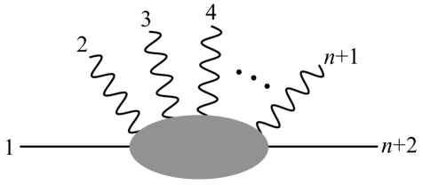
Figure 1: Notation for the $q\overline{q}+ng$ color-ordered amplitude.

However, there is another possible shift in the scalar theory that is allowed in the case of all $+$ gluon amplitudes. This involves a gluon and an external scalar. Consider the $q\overline{q}+ng$ amplitude with the external legs numbered as in Fig. 1. When the gluon $3$ is shifted by

$$3\rangle\to 3\rangle-z\;l_{1}\rangle\ ,$$ (35)

where $l_{1}$ is lightlike, and the external scalar $1$ is shifted by

$$1\to 1+z\;3]\langle l_{1}\ ,$$ (36)

we will show that the all $+$ amplitude scales as $1/z$ for large $z$. Particle 1 is massive, and $l_{1}$ must be defined so that the shifted vector 1 remains on mass shell. This requires

$$\hat{1}^{2}=(1+z\;3]\langle l_{i})^{2}=1^{2}+z[3\,1\,l_{1}\rangle=1^{2}\ ;$$ (37)

that is,

$$[3\,1\,l_{1}\rangle=0\ .$$ (38)

A general solution to this condition is

$$l_{1}=1-{m^{2}\over[3\,1\,3\rangle}3\ ,$$ (39)

that is, that $l_{1}$ is the flatted vector of 1 computed using 3 as a reference vector.

In the fermion theory, this shift could also be defined, but it would restrict the choice of the reference vector for the external fermion to $r=3$ [5]. In the scalar theory, we are free to make this choice of a shift without any restriction on the reference vector that will appear in (32).

We will now prove that the above shift on the legs 1 and 3 has the good $z\to\infty$ behavior that we have claimed. To do this, we consider the possible forms of Feynman diagram that can contribute to an amplitude in this theory with arbitrary numbers of helicity violating vertices. We need only consider the left-most piece of the diagram that contains the scalar line 1 and the gluons 2 and 3. For this, there are two possibilities: either gluon 2 is connected directly to the scalar line and gluon 3 is part of a tree of gluons with external legs $3\cdots k$, or gluons 2 and 3 are part of the same tree of gluons with external legs $2\cdots k$. These cases are shown in Figs. 2 (a) and (b).

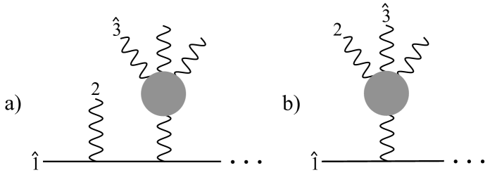
Figure 2: Two classes of diagrams needed to analyze the large $z$ behavior of the 13 shift of the amplitude shown in Fig. 1.

To analyze the trees, we need the explicit expresson for the tree in the case in which all gluons have $+$ helicity. This expression, for the case in which all gluons have the same reference vector $r$, is worked out in the Appendix. The result, for external gluons $j\cdots k$, is

$$J_{a}(j,\cdots,k)=-i{(j+\cdots+k)r\rangle\langle r(j+\cdots+k)\over\langle rj\rangle\langle j(j+1)\rangle\cdots\langle(k-1)k\rangle\langle kr\rangle}\ .$$ (40)

The dangerous term here will be the one that involves the shifted momentum $\hat{3}$ in both terms of the numerator. Note that $\hat{3}$ also appears twice in the denominator, so this term is only of order $z^{0}$.

Now consider the first case, shown in Fig. 2(a). The scalar propagator scales as $z^{-1}$. If we take the gluon 2 to couple via a magnetic moment vertex, the vertex will be of order 1 and the diagram will vanish as $z\to\infty$. Thus, the only dangerous diagram is that in which 2 couples by the ordinary scalar vertex. The leading term in this diagram is

$$i{\langle r\hat{1}2]\over\langle r2\rangle}{i\over\langle 2\hat{1}2]}{-i\ \hat{3}r\rangle\langle r\hat{3}\over\langle r\hat{3}\rangle\langle\hat{3}4\rangle\cdots\langle kr\rangle}\cdots\ .$$ (41)

Notice that the numerator of the last term is a matrix. This is a $2\times 2$ sigma matrix for which we must eventually take the matrix element between the spinors (32) and (33). This term scales as $z^{0}$.

In the second case, the value of the first part of the diagram is just that of the tree (40). The dangerous term is

$$-i{\hat{3}r\rangle\langle r\hat{3}\over\langle r2\rangle\langle 2\hat{3}\rangle\langle\hat{3}4\rangle\cdots\langle kr\rangle}\cdots\ .$$ (42)

These two bad pieces contribute to the amplitude at the same order of $g$ and $a$, and so we may add them together. Then an amazing thing happens. The sum is

$$-i{\hat{3}r\rangle\langle r\hat{3}\over\langle r2\rangle\langle 2\hat{1}2]\langle 2\hat{3}\rangle\langle r\hat{3}\rangle\langle\hat{3}4\rangle\cdots\langle kr\rangle}\cdot[\langle 2\hat{1}2]\langle r\hat{3}\rangle-\langle r\hat{1}2]\langle 2\hat{3}\rangle]\cdots\ .$$ (43)

The quantity in brackets is

$$[2\hat{1}2\rangle\langle r\hat{3}\rangle-[2\hat{1}r\rangle\langle 2\hat{3}\rangle=\langle r2\rangle[2\hat{1}\hat{3}\rangle\ ,$$ (44)

by the Schouten identity. Since the leading $z$ term in $\hat{1}$ and $\hat{3}$ is proportional to the same lightlike vector, this term cancels in the last product. Then the sum of diagrams scales as $z^{-1}$ and the sum has good behavior as $z\to\infty$. This proves our claim that the shift on 1 and 3 generates a BCFW recursion formula for the amplitude with all $+$ helicity gluons.

We now have an algorithm for computing any $q\overline{q}+ng$ amplitude for nonzero $a$. If the amplitude contains both $+$ and $-$ helicity gluons, we can apply $+-$ shifts of the gluons to reduce the amplitude to lower-point components. If the amplitude has only $+$ helicity gluons, we can use the 13 shift above in the scalar theory to reduce the amplitude to lower-point components. If the amplitude has only $-$ helicity gluons, we can use the scalar theory with $\overline{\sigma}\cdot F$. In this theory, a 13 shift that shifts the square bracket of 3 reduces the amplitude to lower-point components. Eventually, the recursion gives the original amplitude in terms of on-shell three-point amplitudes. Though we have given the argument explicitly only for (1), the same strategy works when the QED anomalous magnetic moment interaction (2) is added to the theory.

5 Calculations in the Scalar Theory

Although we have shown that the scalar theory described by (27) or (29) can be effective for computing $q\overline{q}+ng$ amplitudes, some aspects of this theory still appear odd. Of these, the oddest feature is the factor of $1/m$ in front of the Lagrangian. Some diagrams will then contain factors of $1/m$, and one might worry that these would generate bad behavior in the limit $m\to 0$. In this section, we will display some amplitudes in the theory (29) that might provide sanity checks on the use of that expression.

First, consider three-point amplitudes. The scalar amplitude as a $2\times 2$ matrix is

$${\cal A}_{s}(1,2^{+},3)={g\over m}\biggl{[}{\langle r12]\langle s32]\over\langle s31r\rangle+m^{2}\langle sr\rangle}+{\hat{g}_{L}\over 2}2][2\biggr{]}\ ,$$ (45)

where $r$ and $s$ are the reference spinors for particles 1 and 3, respectively. Setting $\hat{g}_{L}=2$, the fermion amplitudes can be computed by taking matrix elements in (32) and (33). We find

$${\cal A}(1^{+},2^{+},3^{+}) = {gm\over\langle r1^{\flat}\rangle\langle 3^{\flat}s\rangle}{\langle sr\rangle\langle r12]\langle s32]\over\langle s31r\rangle+m^{2}\langle sr\rangle}\ ,$$ (46)

$${\cal A}(1^{+},2^{+},3^{-}) = -g{[1^{\flat}2]^{2}\over[1^{\flat}3^{\flat}]}-{gm^{2}\over\langle r1^{\flat}\rangle\langle s3s]}{\langle rs\rangle[1^{\flat}s]\over[1^{\flat}3^{\flat}]}{\langle r12]\langle s32]\over\langle s31r\rangle+m^{2}\langle sr\rangle}\ ,$$ (47)

$${\cal A}(1^{-},2^{+},3^{+}) = g{[23^{\flat}]^{2}\over[1^{\flat}3^{\flat}]}+{gm^{2}\over\langle r1r]\langle 3^{\flat}s\rangle}{\langle rs\rangle[r3^{\flat}]\over[1^{\flat}3^{\flat}]}{\langle r12]\langle s32]\over\langle s31r\rangle+m^{2}\langle sr\rangle}\ ,$$ (48)

$${\cal A}(1^{-},2^{+},3^{-}) = -gm{[r2][2s]\over[r1^{\flat}][3^{\flat}s]}-gm{[rs]\over[r1^{\flat}][3^{\flat}s]}{\langle r12]\langle s32]\over\langle s31r\rangle+m^{2}\langle sr\rangle}\ .$$ (49)

These expressions are in agreement with explicit QCD calculations. Taking the limit $m\to 0$, these expressions reduce to the familiar three point maximal helicity violating (MHV) amplitudes

$${\cal A}(1^{+},2^{+},3^{-}) = -g{[12]^{2}\over[13]}\ ,$$ (50)

$${\cal A}(1^{-},2^{+},3^{+}) = g{[23]^{2}\over[13]}\ ,$$ (51)

with ${\cal A}(1^{+},2^{+},3^{+})={\cal A}(1^{-},2^{-},3^{-})=0$.

At four points, there exist two helicity configurations of the gluons that cannot be related by parity. These amplitudes can be computed in the scalar theory; we find

$${\cal A}_{s}(1,2^{+},3^{+},4) = g^{2}m{[32]\over\langle 2123\rangle}+{g^{2}\hat{g}_{L}\over 2m}\biggl{(}{m^{2}\ 2][3\over\langle 2123\rangle}+{12\rangle[32][2\over\langle 2123\rangle}+{412][3\over\langle 2123\rangle}+{\hat{g}_{L}\over 2}{2][23][3\over\langle 212]}\biggr{)}$$

$${\cal A}_{s}(1,2^{+},3^{-},4) = -{g^{2}\over m}{\langle 312]^{2}\over\langle 212]\langle 232]}-{g^{2}\hat{g}_{L}\over 2m}{\langle 312]\over\langle 212][23]}2][2\ .$$ (52)

To compare to fermion amplitudes, we need to take matrix elements of these $2\times 2$ matrices. For brevity, we will only consider the $\hat{g}_{L}=2,$ $m=0$ case. For the case with both gluons with $+$ helicity, the massless fermion amplitude with any helicity configuration for the fermions must vanish. For massless fermions, the $--$ fermion projection explicitly vanishes. Multiplying this scalar amplitude by $[a$ on the left and $b]$ on the right and simplifying yields

$$[a\ {\cal A}_{s}(1,2^{+},3^{+},4)\ b]={g^{2}\over m}{\langle 41\rangle[23][4b][1a]\over\langle 212]\langle 23\rangle}\ .$$ (53)

This indeed vanishes if either $1$ or $4$ have $+$ helicity.

In the second case, in which the gluons have opposite helicity, the projection should yield the familiar MHV amplitudes at four points. If we choose both particles 1 and 4 to have $+$ helicity, the projection vanishes by momentum conservation. If instead, particles 1 and 4 have opposite helicity, the projection yields

$${\cal A}(1^{+},2^{+},3^{-},4^{-}) = g^{2}{\langle 13\rangle\langle 34\rangle^{3}\over\langle 12\rangle\langle 23\rangle\langle 34\rangle\langle 41\rangle}\ ,$$ (54)

$${\cal A}(1^{-},2^{+},3^{-},4^{+}) = g^{2}{\langle 13\rangle^{3}\langle 34\rangle\over\langle 12\rangle\langle 23\rangle\langle 34\rangle\langle 41\rangle}\ ,$$ (55)

which agree with the standard results.

As discussed in the previous section, the all $+$ helicity amplitudes are completely described by this theory. In fact, from the amplitude in (52), one can verify that, order by order in $a$, this expression agrees with that calculated using from (1). However, a simple observation on the opposite helicity amplitude in (52) shows that this amplitude cannot reproduce the full result from (1). The result above contains only terms proportional to $a^{0}$ and $a^{1}$, while the exact answer would also contain a term proportional to $a^{2}$. This discrepancy is expected, and it is not troublesome for us, since this amplitude in the original theory can be constructed using BCFW directly.

There is one more interesting cross check that we have made of the form of (29). For $\hat{g}_{L}=2$, $a=0$, and so (29) gives an exact description of (1) for all gluon helicity states. At the same time, for $a=0$, all amplitudes of (1) can be computed by BCFW shifts on gluons with the helicity combinations $+-$, $++$, $--$. Thus, one can compute every $q\overline{q}+ng$ amplitude in two ways, first, from (1) using gluon shifts only and, second, from (29), using the 13 shift described in the previous section. We have checked equality numerically to 6 significant figures for all of these amplitudes up to $n=8$ gluons.

6 Conclusion

We have shown that the BCFW recursion relations can be used to compute all amplitudes in a theory with an anomalous magnetic moment. The prescription for using BCFW is as follows:

1. If an amplitude contains at least one $-$ and one $+$ helicity gluon, use the $+-$ shift to compute amplitudes in the theory defined by

   $${\cal L}=\overline{\Psi}(i\not{\hbox{\kern-4.0pt$D$}}-m)\Psi+{ga\over 2m}\overline{\Psi}\Sigma_{\mu\nu}F^{\mu\nu a}t^{a}\Psi\ .$$ (56)

2. If an amplitude contains only $+$ helicity gluons, shift on the scalar and a non-adjacent gluon to compute amplitudes in the theory defined by

   $${\cal L}={1\over m}\overline{\psi}^{\dagger}\biggl{[}-D^{2}-m^{2}+i{g\hat{g}_{L}\over 2}\sigma_{\mu\nu}F^{\mu\nu a}t^{a}\biggr{]}\psi\ .$$ (57)

   The gluon momentum should be shifted in the angle bracket. To compute the amplitude with external fermions, project onto the fermion line by multiplying by the appropriate wavefunctions on the left and right.

3. If an amplitude contains only $-$ helicity gluons, shift on the scalar and a non-adjacent gluon to compute amplitudes in the theory defined by

   $${\cal L}={1\over m}\overline{\psi}\biggl{[}-D^{2}-m^{2}+i{g\hat{g}_{L}\over 2}{\overline{\sigma}}_{\mu\nu}F^{\mu\nu a}t^{a}\biggr{]}\psi^{\dagger}\ .$$ (58)

   The gluon momentum should be shifted in the square bracket. To compute the amplitude with external fermions, project onto the fermion line by multiplying by the appropriate wavefunctions on the left and right.

We have shown that this is an efficient algorithm for computation of tree amplitudes. We hope to present some phenomenological applications of this method soon.

Our conclusions include the statement that the BCFW recursion formula cannot be used to fully construct amplitudes in the original fermion theory. This apparently contradicts a result of [12], although in fact the anomalous magnetic moment coupling falls outside the hypotheses of that paper [13]. More generally, the validity of BCFW recursion must be thought through carefully for effective theories with nonrenormalizable couplings. However, our analysis indicates that remedies for their bad large-momentum behavior can be found in some cases.

A distinct momentum shift useful for studying generic theories was introduced in [14]. Instead of only shifting the momenta of two of the particles in an amplitude, the authors consider shifting the momentum of all external particles. Explicitly, for an amplitude with all massless particles, the shift can be expressed as

$$i\rangle\to i\rangle+w_{i}\ z\ X\rangle.$$ (59)

$i$ is any external particle in the amplitude, $X$ is an arbitrary, massless four-vector and the coefficients $w_{i}$ are chosen to conserve momentum:

$$\sum_{i}w_{i}\ i]=0.$$ (60)

The dependence on the parameter $z$ is easily determined by considering the dimension and helicity constraints on an amplitude in a generic theory. For the case of the shift in (59), the amplitude behaves as

$${\cal A}\sim z^{s}\mbox{ as }z\to\infty\mbox{ with }2s=4-n-c-H,$$ (61)

where $n$ is the number of external legs, $c$ is the sum of dimensions of coupling constants in an amplitude and $H$ is the sum of helicities of external particles. An on-shell recursion exists when $s<0$; in that case, there are more angle brackets in the denominator of an amplitude than in the numerator. In the anomalous magnetic moment theory, this all-leg shift leads to a recursion relation precisely for those amplitudes for which BCFW fails. This is easily seen at the four point level from (19) and (20). In (19), the amplitude is constructible with this shift because there is one angle bracket in the denominator and none in the numerator, while in (20) there is one more angle bracket in the numerator and so this amplitude is not constructible. This all-leg shift could be another way to compute amplitudes in a theory with an anomalous magnetic moment. Unfortunately, its practical use is limited because of the proliferation of cuts that one needs to compute.

Recently, there has been some interest in the literature in finding classes of theories in whose amplitudes are constructible using BCFW [15, 16]. The hope has been that the validity of the BCFW recursion formula would say something about the behavior of the theory at high energy. It is remarkable that amplitudes in Einstein gravity and, equivalently, in ${\cal N}=8$ supergravity, are are constructible using BCFW [17, 18]. It has been hoped that this property is evidence for special simplicity of the ${\cal N}=8$ theory. Further speculations on this point ought to take into account, one way or the other, our result that QCD with an anomalous magnetic moment is also BCFW constructible. We hope that the methods discussed here can be used to study other realistic or effective theories, and that those investigations will shed more light on the high-momentum behavior of non-renormalizable theories.

Appendix A All-$+$ gluon helicity amplitude for massless quarks

For massless particles, we have found an explicit formula for the $q\overline{q}+ng$ amplitudes with all $+$ helicity gluons. The derivation of this formula makes use of the off-shell current formalism of Berends and Giele [3]. The off-shell current with all $+$ helicities is needed for other arguments in this paper, in particular, in the analysis of the large $z$ behavior of the scalar theory at the end of Section 4.

We consider an amplitude with a single massless fermion line and $n$ $+$ helicity gluons. We would like to compute the correction to the standard QCD result coming from the presence of an anomalous magnetic moment. Since the background field with only $+$ helicity gluons is self-dual, the $\overline{\sigma}\cdot F$ piece of the magnetic moment operator gives zero and only the $\sigma\cdot F$ of this operator contributes to the amplitude. This term has a matrix element only between a $+$ helicity fermion and a $+$ helicity antifermion. All propagators and all other vertices in the diagram are helicity-conserving. This means that, for the amplitude to be non-zero, the helicity of both external fermions must be $+$ and there must be exactly one insertion of the magnetic moment operator.

The magnetic moment operator contains both a three-point and a four-point vertex. Both terms contribute to the Berends-Giele current. The terms simplify, however, if we choose all of the $+$ helicity gluons to have the same reference vector $r$. Our analysis here generalizes the results of Berends and Giele [3] obtained for currents with standard QCD vertices.

Consider first the term from the four-point vertex. Computing the first few trees emanating from the four-point vertex, we find

$$J_{4}(1,2) = i{(1+2)^{2}\over\langle r1\rangle\langle 12\rangle\langle 2r\rangle}\>r\rangle\langle r\ ,$$ (62)

$$J_{4}(1,2,3) = i{(1+2+3)^{2}\over\langle r1\rangle\langle 12\rangle\langle 23\rangle\langle 3r\rangle}\>r\rangle\langle r\ .$$ (63)

From these expressions, we postulate the general form of this term:

$$J_{4}(1,\ldots,n)=i{(1+\cdots+n)^{2}\over\langle r1\rangle\langle 12\rangle\cdots\langle nr\rangle}\>r\rangle\langle r\ .$$ (64)

To prove this, note that the BCFW recursion is valid for shifting on any two gluons. Thus, to prove the general expression, shift gluons 2 and 3 and use induction. Only one term contributes in the BCFW sum and it is given by the above equation.

Similarly, one can compute the first few all $+$ gluon trees that emanate from the three point helicity violating vertex:

$$J_{3}(1) = -i1][1=-i{(1)r\rangle\langle r(1)\over\langle r1\rangle\langle 1r\rangle}\ ,$$ (65)

$$J_{3}(1,2) = -i{(1+2)r\rangle\langle r(1+2)\ +\ (1+2)^{2}\;r\rangle\langle r\over\langle r1\rangle\langle 12\rangle\langle 2r\rangle}\ ,$$ (66)

$$J_{3}(1,2,3) = -i{(1+2+3)r\rangle\langle r(1+2+3)\ +\ (1+2+3)^{2}\;r\rangle\langle r\over\langle r1\rangle\langle 12\rangle\langle 23\rangle\langle 3r\rangle}\ .$$ (67)

These suggest a general form,

$$J_{3}(1,\ldots,n)=-i{(1+\cdots+n)r\rangle\langle r(1+\cdots+n)+(1+\cdots+n)^{2}\;r\rangle\langle r\over\langle r1\rangle\langle 12\rangle\cdots\langle nr\rangle}\ .$$ (68)

and that can again be established by induction.

Note that the first term in the numerator in (68) gives a matrix element between a $+$ helicity fermion and $+$ helicity antifermion. The second term gives a matrix element between a $-$ helicity fermion and a $-$ helicity antifermion. However, this latter term, proportional to the total mass of the gluons in the tree, cancels neatly against (64). Finally, we find

$$J_{a}(1,\ldots,n)=J_{3}(1,\ldots,n)+J_{4}(1,\ldots,n)=-i{(1+\cdots+n)r\rangle\langle r(1+\cdots+n)\over\langle r1\rangle\langle 12\rangle\cdots\langle nr\rangle}\ .$$ (69)

This result for the Berends-Giele current of all $+$ helicity gluons is quoted in (40) and forms the basis for our analysis at the end of Section 4.

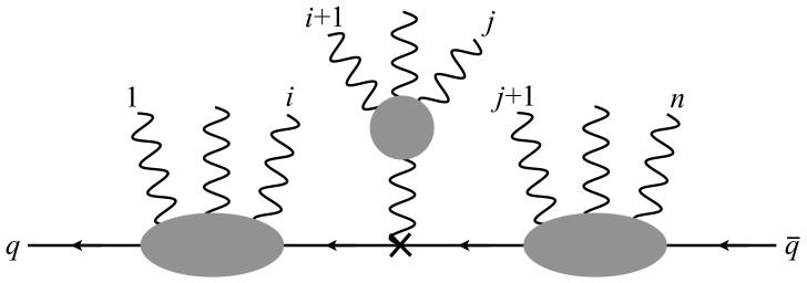
Figure 3: Generic form of a $q\overline{q}+ng$ amplitude for massless fermions with a magnetic moment vertex and all $+$ helicity gluons. The cross represents the magnetic moment vertex.

In the case of massless QCD with a single helicity violating vertex, the amplitude has the diagrammatic form shown in Fig. 3. We can write the gauge invariant amplitude as

$${\cal A}(q^{+},g_{1}^{+},\ldots,g_{n}^{+},\overline{q}^{+})={g^{n}a\over 2M}\sum_{0\leq i<j\leq n}\not{\hbox{\kern-2.0pt$J$}}(q;1,\ldots,i)\not{\hbox{\kern-2.0pt$J$}}_{a}(i+1,\ldots,j)\not{\hbox{\kern-2.0pt$J$}}(j+1,\ldots,n;\overline{q})\ .$$ (70)

Here, the factors $J$ are currents with an off-shell fermion leg and any number of gluons. These were first found by Berends and Giele in [3]. The factor $J_{a}$ is the current from a magnetic moment vertex discussed above. The explicit forms for the currents $J$ are

$$\not{\hbox{\kern-2.0pt$J$}}(q;1,\ldots,i)=-{\langle r(1+\cdots i+q)\over\langle q1\rangle\langle 12\rangle\cdots\langle ir\rangle}$$ (71)

and

$$\not{\hbox{\kern-2.0pt$J$}}(j+1,\ldots,n;\overline{q})=-{((j+1)+\cdots+n+\overline{q})r\rangle\over\langle r(j+1)\rangle\cdots\langle n\overline{q}\rangle}\ .$$ (72)

The amplitude we wish to compute is the sum over all possible insertions of the helicity violating vertex with $j-i$ gluons off of the helicity violating vertex and $i$ and $n-j$ to the left and right of the helicity violating vertex, respectively.

Plugging in the various pieces, the amplitude becomes

$${\cal A}(q^{+},g_{1}^{+},\ldots,g_{n}^{+},\overline{q}^{+})={g^{n}a\over 2M}\sum_{0\leq i<j\leq n}\!\!{\langle r(q+1+\cdots+i)((i+1)+\cdots+j)r\rangle^{2}\over\langle q1\rangle\cdots\langle ir\rangle\langle r(i+1)\rangle\cdots\langle jr\rangle\langle r(j+1)\rangle\cdots\langle n\overline{q}\rangle}\ ,$$ (73)

where momentum conservation has been used. For $n=2$, this equation agrees with the expression in (19). This expression is gauge invariant as well. It is important to note that gauge invariance follows only after summing over all possible places of insertion of the magnetic moment vertex. In massless QCD, this is the end of the story. We have explicitly constructed the amplitude with all $+$ helicity gluons and on all other amplitudes, one can use BCFW to construct amplitudes.

Since the amplitude in (73) involves only $+$ helicity gluons, it is also possible to look at this amplitude as a solution for the motion of a massless fermion in a purely self-dual background field. For such backgrounds, Rosly and Selivanov [19] have developed a special formalism, called the perturbiner method, for amplitude computations. In this method, they solve the Yang-Mills equations recursively in the number of gluons, then use that solution to evaluate the fermion propagator. Their solution can be written as

$$A_{\mu}=i\sum_{i=0}^{\infty}{\langle r\gamma_{\mu}(1+2+\cdots+i)r\rangle\over\langle r1\rangle\langle 12\rangle\cdots\langle ir\rangle}{\cal E}_{1}{\cal E}_{2}\cdots{\cal E}_{i}\ ,$$ (74)

for color-ordered gluons, with $r$ the common reference vector for all of the gluons. The objects ${\cal E}_{n}$ are the solutions to the free equations of motion,

$${\cal E}_{n}=a_{n}t_{n}e^{ik_{n}\cdot x}\ ,$$

where $a_{n}$ is the nilpotent creation operator and $t_{n}$ is the color matrix. The coefficients of the product of ${\cal E}$s are the Berends-Giele off-shell currents for all $+$ helicity gluon configurations. Applying (74) to the magnetic moment vertex gives an alternative derivation of (69).

This analysis becomes much more complex in the case of massive fermions. In the massive case, the fermion propagators now have helicity-violating factors, and so we can insert any number of magnetic moment vertices into an amplitude. In principle, we can still construct the all $+$ gluon amplitude with the stitching procedure used in the massless case. However, to do this, we need to know an explicit form for the analog of the off-shell current in (71) for massive fermions. In addition, we would need to know this current for both helicities of the massive fermion. We do not show them here as their form is not illuminating. However, rather than suggesting a general form for this current, the expressions seem to get only more complicated as the number of gluons increases. It seems that for massive fermions, this method is not useful for determining the amplitude with all $+$ helicity gluons.

ACKNOWLEDGEMENTS

The authors thank Jared Kaplan for helpful discussions of many parts of our formalism. A. L. thanks the University of Durham Institute for Particle Physics Phenomenology for their tea and hospitality while some of this work was completed. This work is supported by the US Department of Energy under contract DE–AC02–76SF00515.

References

- [1] D. Atwood, A. Kagan and T. G. Rizzo, Phys. Rev. D 52, 6264 (1995) [arXiv:hep-ph/9407408]; T. G. Rizzo, Phys. Rev. D 51, 3811 (1995) [arXiv:hep-ph/9409460].
- [2] P. Haberl, O. Nachtmann and A. Wilch, Phys. Rev. D 53, 4875 (1996) [arXiv:hep-ph/9505409].
- [3] F. A. Berends and W. T. Giele, Nucl. Phys. B 306, 759 (1988).
- [4] R. Britto, F. Cachazo and B. Feng, Nucl. Phys. B 715, 499 (2005) [arXiv:hep-th/0412308]; R. Britto, F. Cachazo, B. Feng and E. Witten, Phys. Rev. Lett. 94, 181602 (2005) [arXiv:hep-th/0501052].
- [5] C. Schwinn and S. Weinzierl, JHEP 0704, 072 (2007) [arXiv:hep-ph/0703021].
- [6] L. J. Dixon, arXiv:hep-ph/9601359; M. L. Mangano and S. J. Parke, Phys. Rept. 200, 301 (1991).
- [7] J. D. Bjorken, J. B. Kogut, D. E. Soper, Phys. Rev. D3, 1382 (1971); J. B. Kogut, D. E. Soper, Phys. Rev. D1, 2901-2913 (1970).
- [8] S. J. Brodsky, H. -C. Pauli, S. S. Pinsky, Phys. Rept. 301, 299-486 (1998). [hep-ph/9705477]; R. Venugopalan, [nucl-th/9808023]; H. Leutwyler, Nucl. Phys. B76, 413-444 (1974).
- [9] C. W. Bauer, S. Fleming, D. Pirjol, I. W. Stewart, Phys. Rev. D63, 114020 (2001). [hep-ph/0011336].
- [10] W. A. Bardeen, Prog. Theor. Phys. Suppl. 123, 1 (1996).
- [11] To see explicitly that in an external state of all positive helicity gluons, see (69).
- [12] C. Cheung, JHEP 1003, 098 (2010). [arXiv:0808.0504 [hep-th]].
- [13] C. Cheung, private communication.
- [14] T. Cohen, H. Elvang, M. Kiermaier, [arXiv:1010.0257 [hep-th]].
- [15] P. Benincasa and F. Cachazo, arXiv:0705.4305 [hep-th].
- [16] H. Elvang, “On the structure of scattering amplitudes”, talk given at Stanford University, January 25, 2010
- [17] N. Arkani-Hamed and J. Kaplan, JHEP 0804, 076 (2008) [arXiv:0801.2385 [hep-th]].
- [18] J. Bedford, A. Brandhuber, B. J. Spence and G. Travaglini, Nucl. Phys. B 721, 98 (2005) [arXiv:hep-th/0502146]; F. Cachazo and P. Svrcek, arXiv:hep-th/0502160; P. Benincasa, C. Boucher-Veronneau and F. Cachazo, JHEP 0711, 057 (2007) [arXiv:hep-th/0702032].
- [19] A. A. Rosly and K. G. Selivanov, Phys. Lett. B 399, 135 (1997) [arXiv:hep-th/9611101].