Relation between the $0\nu\beta\beta$ and $2\nu\beta\beta$ nuclear matrix elements revisited

Abstract

We show that the dominant Gamow-Teller part, $M^{0\nu}_{GT}$, of the nuclear matrix element governing the neutrinoless $\beta\beta$ decay is related to the matrix element $M^{2\nu}_{cl}$ governing the allowed two-neutrino $\beta\beta$ decay. That relation is revealed when these matrix elements are expressed as functions of the relative distance $r$ between the pair of neutrons that are transformed into a pair of protons in the $\beta\beta$ decay. Analyzing this relation allows us to understand the contrasting behavior of these matrix elements when $A$ and $Z$ is changed; while $M^{0\nu}_{GT}$ changes slowly and smoothly, $M^{2\nu}$ has pronounced shell effects. We also discuss the possibility of phenomenological determination of the $M^{2\nu}_{cl}$ and from them of the $M^{0\nu}_{GT}$ values from the experimental study of the $\beta^{\pm}$ strength functions.

I Introduction

Observing $0\nu\beta\beta$ decay would tell us that the total lepton number is not a conserved quantity, and that neutrinos are massive Majorana fermions. Answering these questions is obviously a crucial part of the search for the “Physics Beyond the Standard Model”. Consequently, experimental searches for the $0\nu\beta\beta$ decay, of ever increasing sensitivity, are pursued worldwide (for a recent review of the field, see e.g. AEE ). However, interpreting existing results as a determination of the neutrino effective mass, and planning new experiments, is impossible without the knowledge of the corresponding nuclear matrix elements. Their determination, and a realistic estimate of their uncertainty, are therefore an integral part of the problem.

The nuclear matrix elements $M^{0\nu}$ of the $0\nu\beta\beta$ decay must be evaluated using tools of nuclear structure theory. Unfortunately, there are no observables that could be simply and directly linked to the magnitude of $0\nu\beta\beta$ nuclear matrix elements and that could be used to determine them in an essentially model independent way. In the past, knowledge of the $2\nu\beta\beta$-decay rate, and therefore of the corresponding matrix elements $M^{2\nu}$, and of the ordinary $\beta$ decay $ft$ values and the corresponding beta strength distributions, were used to constrain the nuclear model parameters, in particular when the Quasiparticle Random Phase Approximation (QRPA) was employed us1 ; us2 ; us3 ; SC . In the present paper we discuss a novel relation between these nuclear matrix elements.

Very early, Primakoff and Rosen Pri59 speculated that since the operators governing $0\nu\beta\beta$ and $2\nu\beta\beta$ decays differ by a relatively gentle radial dependence, approximately of the form $1/r_{ij}$, the corresponding matrix elements might be proportional to each other with the proportionality constant $\sim 1/R$, where $R=1.2A^{1/3}$fm is the nuclear radius. At that time the authors also believed that the $2\nu\beta\beta$ decay can be treated in closure, thus that the corresponding matrix element is dimensionless, while in fact the realistic $2\nu\beta\beta$ matrix element has dimension energy^-1. Also, the $0\nu\beta\beta$ matrix elements are now, by convention, made dimensionless by including the nuclear radius $R$ as a multiplicative factor, which is compensated by the factor $R^{-2}$ in the corresponding phase space function $G^{0\nu}$.

Modern nuclear structure evaluations of these matrix elements do not support the conjecture of proportionality between $M^{0\nu}$ and $M^{2\nu}$. The rate of the $2\nu\beta\beta$ decay has been determined experimentally in many nuclei, and hence the $2\nu\beta\beta$ matrix elements $M^{2\nu}$ are known. They exhibit pronounced shell effects and vary rather abruptly between nuclei with different $Z$ and $A$. At the same time, the calculated $0\nu\beta\beta$ nuclear matrix elements, whether based on the QRPA us1 ; us2 ; us3 ; SC , nuclear shell model Men08 ; Cau08 ; Cau08a , or the Interacting Boson Model Bar09 , do not show such a variability; instead they vary relatively smoothly between nuclei with different $Z,A$. The reason for the difference is, presumably, the very different momentum transfer $q$ involved in these matrix elements, even though they involve the same initial and final nuclear states. In the $2\nu\beta\beta$ decay the momentum transfer $q$ is restricted to $q<Q$, where $Q$ is the energy difference of the initial and final atomic masses. Hence, the allowed approximation is valid, $qR\ll 1$, and only the Gamow-Teller operator ${\mathbf{\sigma}}\tau_{+}$ and only the $1^{+}$ virtual intermediate states, contribute. On the other hand, in the $0\nu\beta\beta$ decay the momentum transfer is of the order of the nucleon Fermi momentum $q\sim 200$ MeV, $qR\geq 1$, and all $J^{\pi}$ virtual intermediate states can contribute significantly. Our discussion here sheds more light on the different behavior of the $0\nu\beta\beta$ and $2\nu\beta\beta$ matrix elements.

It is worthwhile to remember another type of relation, explored in the classic paper by Pontecorvo Pon68 . At that time the available information on $\beta\beta$ decay was based on the geochemical determination of the total decay rate, $1/\tau_{tot}=1/\tau_{0\nu}+1/\tau_{2\nu}$. Since these two modes scale very differently with $Q$ ($\sim Q^{5}$ for $0\nu$ and $\sim Q^{11}$ for $2\nu$) Pontecorvo suggested that comparing the total lifetimes of two isotopes, ¹³⁰Te and ¹²⁸Te, which have very different $Q$ values, might reveal the presence of the lepton number violating $0\nu$ decay, provided the nuclear matrix elements of these two isotopes are identical. While the matrix elements of these two isotopes are indeed rather close, they are not quite the same. Moreover, we know today that the $0\nu$ decay rate is very much smaller, if it is indeed nonvanishing, than the $2\nu$ decay rate.

The present paper is structured as follows. In the next section II we describe the formalism that leads to the relation between the Gamow-Teller part of the $0\nu\beta\beta$ matrix element and the $2\nu\beta\beta$ matrix element evaluated in the closure approximation. We also discuss the validity of the closure approximation in the $0\nu\beta\beta$ case. In the following section III we discuss this novel relation in more detail and show numerous examples. In section IV we briefly discuss the issue of quenching of the axial current matrix elements. While closure is a rather poor approximation in the $2\nu\beta\beta$ case, we argue in section V that combining the known lifetimes with the often measured distribution of the $\beta^{-}$ and $\beta^{+}$ strengths constrains the $M^{2\nu}_{cl}$ values substantially. We believe that the relation found here allows one to better understand the different behavior of these matrix elements. We conclude in the last section.

II Formalism

Assuming that the $0\nu\beta\beta$ decay is caused by the exchange of the light Majorana neutrinos, the halflife and the nuclear matrix element are related through

$$\frac{1}{T_{1/2}}=G^{0\nu}(Q,Z)|M^{0\nu}|^{2}~{}|\langle m_{\beta\beta}\rangle|^{2}~{},$$ (1)

where $G^{0\nu}(Q,Z)$ is the easily calculable phase space factor, $\langle m_{\beta\beta}\rangle$ is the effective neutrino Majorana mass whose determination is the ultimate goal of the experiments, and $M^{0\nu}$ is the nuclear matrix element consisting of Gamow-Teller, Fermi and Tensor parts,

$$M^{0\nu}=M^{0\nu}_{GT}-\frac{M^{0\nu}_{F}}{g_{A}^{2}}+M^{0\nu}_{T}\equiv M^{0\nu}_{GT}(1+\chi_{F}+\chi_{T})~{},$$ (2)

where $\chi_{F}$ and $\chi_{T}$ are the matrix element ratios that are smaller than unity and, presumably, less dependent on the details of the applied nuclear model. In the following we concetrate on the GT part, $M^{0\nu}_{GT}$, which can be somewhat symbolically written as

$$M^{0\nu}_{GT}=\langle f|\Sigma_{lk}{\mathbf{\sigma}}_{l}\cdot{\mathbf{\sigma}}_{k}\tau_{l}^{+}\tau_{k}^{+}H(r_{lk},\bar{E})|i\rangle~{},$$ (3)

where $H(r_{lk},\bar{E})$ is the neutrino potential described in detail below and $r_{lk}$ is the relative distance between the two neutrons that are trasformed in the decay into the two protons.

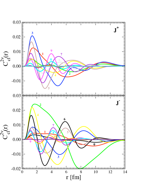
Figure 1: Multipole decomposition of $C^{2\nu}_{cl}(r)$ as function of relative distance of two $\beta$-decaying neutrons in the ${}^{76}Ge$ nucleus. Calculation performed for ⁷⁶Ge with 23 single particle levels model space. Positive parity multipoles are shown in the upper panel and the negative parity ones in the lower panel. (color online)

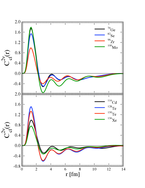
Figure 2: $C^{2\nu}_{cl}(r)$ as a function of the relative distance of the decaying neutron pair for different nuclei. (color online)

In Ref. us3 , based on the QRPA, as well as in Ref. Men08 based on the nuclear shell model, the function $C^{0\nu}(r)$ that describes the dependence of the $M^{0\nu}$ on the distance $r_{lk}$ was introduced. Formally, this function can be defined as EV04

$$C^{0\nu}_{GT}(r)=\langle f|\Sigma_{lk}{\mathbf{\sigma}}_{l}\cdot{\mathbf{\sigma}}_{k}\tau_{l}^{+}\tau_{k}^{+}\delta(r-r_{lk})H(r_{lk},\bar{E})|i\rangle~{},$$ (4)

where $\delta(x)$ is the Dirac delta function. Obviously, this function is normalized by

$$M^{0\nu}_{GT}=\int_{0}^{\infty}C^{0\nu}_{GT}(r)dr~{},$$ (5)

and has the dimension lenght^-1. The shape of $C^{0\nu}_{GT}(r)$ is very similar in both QRPA and NSM and in all cases consists of a peak with maximum at $r\sim 1$ fm ending near $r\sim 2.5$ fm, and of very little contributions for larger values of $r$.

Now lets turn to the case of the $2\nu$ decay mode. The matrix element $M^{2\nu}$ governing the $2\nu\beta\beta$ decay mode is of the form

$$M^{2\nu}=\Sigma_{m}\frac{\langle f||\sigma\tau^{+}||m\rangle\langle m||\sigma\tau^{+}||i\rangle}{E_{m}-(M_{i}+M_{f})/2}~{},$$ (6)

where the sumation extends over all $1^{+}$ virtual intermediate states. We can introduce also the closure analog of $M^{2\nu}$, denoted by $M^{2\nu}_{cl}$, by replacing the energies $E_{m}$ by a properly defined average value $\bar{E}_{2\nu}$. Thus,

$$M^{2\nu}_{cl}\equiv\langle f|\Sigma_{lk}{\mathbf{\sigma}}_{l}\cdot{\mathbf{\sigma}}_{k}\tau_{l}^{+}\tau_{k}^{+}|i\rangle~{},$$

$$M^{2\nu}_{cl}=M^{2\nu}\times(\bar{E}_{2\nu}-(M_{i}+M_{f})/2)~{}.$$ (7)

In analogy with Eq. (4) we can define the new function

$$C^{2\nu}_{cl}(r)=\langle f|\Sigma_{lk}{\mathbf{\sigma}}_{l}\cdot{\mathbf{\sigma}}_{k}\delta(r-r_{lk})\tau_{l}^{+}\tau_{k}^{+}|i\rangle~{},$$

$$M^{2\nu}_{cl}=\int_{0}^{\infty}C^{2\nu}_{cl}(r)dr~{}.$$ (8)

While the matrix elements $M^{2\nu}$ and $M^{2\nu}_{cl}$ get contributions only from the $1^{+}$ intermediate states, the function $C^{2\nu}_{cl}$ gets contributions from all intermediate multipoles. This is the consequence of the $\delta$ function in the definition of $C^{2\nu}_{cl}(r)$. When expanded, all multipoles contribute. Naturally, when integrated over $r$ only the contributions from the $1^{+}$ are nonvanishing. An example of the multipole decomposition of $C^{2\nu}_{cl}(r)$ is shown in Fig. 1, and in Fig. 2 we show the functions $C^{2\nu}_{cl}(r)$ for a variety of $\beta\beta$ decaying nuclei.

For completeness we show here the QRPA formula used for the evaluation of the function $C^{2\nu}_{cl}(r)$ and its multipole decomposition depicted in Fig. 1. First, the function

$$f^{\mathcal{J}}_{n,n^{\prime},p,p^{\prime}}(r)=$$ (9)

$$\langle p(1),p^{\prime}(2)(r);{\mathcal{J}}\parallel{\mathbf{\sigma_{1}}}\cdot{\mathbf{\sigma_{2}}}\parallel n(1),n^{\prime}(2)(r);{\mathcal{J}}\rangle$$

is introduced where $r$ is the relative distance between the neutrons in the states $n$ and $n^{\prime}$, respectively protons in $p$ and $p^{\prime}$. Then, the part of $C^{2\nu}_{cl}(r)$ with the multipolarity $J^{\pi}$ is given by

$$C^{2\nu}_{cl}(r,J^{\pi})=\sum_{k_{i},k_{f},\mathcal{J}}\sum_{pnp^{\prime}n^{\prime}}(-1)^{j_{n}+j_{p^{\prime}}+J^{\pi}+{\mathcal{J}}}$$

$$\times\sqrt{2{\mathcal{J}}+1}\times\left\{\begin{array}[]{c c c}j_{p}&j_{n}&J^{\pi}\\ j_{n^{\prime}}&j_{p^{\prime}}&{\mathcal{J}}\end{array}\right\}\times f^{\mathcal{J}}_{n,n^{\prime},p,p^{\prime}}(r)\times$$ (12)

$$\langle 0_{f}^{+}||[\widetilde{c_{p^{\prime}}^{+}\tilde{c}_{n^{\prime}}}]_{J}||J^{\pi}k_{f}\rangle\langle J^{\pi}k_{f}|J^{\pi}k_{i}\rangle\langle J^{\pi}k_{i}||[c_{p}^{+}\tilde{c}_{n}]_{J}||0_{i}^{+}\rangle.$$

Here $k_{i}$ and $k_{f}$ are the labels of the excited states with the multipolarity $J^{\pi}$ in the intermediate nucleus built on the initial and final nuclear ground states, and $\langle 0_{f}^{+}||[{c_{p^{\prime}}^{+}\tilde{c}_{n^{\prime}}}]_{J}||J^{\pi}k_{f}\rangle$ and $\langle J^{\pi}k_{i}||[c_{p}^{+}\tilde{c}_{n}]_{J}||0_{i}^{+}\rangle$ are the corresponding QRPA amplitudes.

It is now clear that, by construction,

$$C^{0\nu}_{GT}(r)=H(r,\bar{E})\times C^{2\nu}_{cl}(r)~{},$$ (13)

which is valid for any shape of the neutrino potential $H(r,\bar{E})$. Thus, if $C^{2\nu}_{cl}(r)$ is known, $C^{0\nu}_{GT}(r)$ and therefore also $M^{0\nu}_{GT}$ can be easily determined. The equation (13) represents the basic relation between the $0\nu$ and $2\nu$ $\beta\beta$-decay modes that we will explore further.

Note that while the function $C^{2\nu}_{cl}(r)$ has a substantial negative tail past $r\sim 2-3$ fm, these distances contribute very little to $C^{0\nu}_{GT}(r)$. This is a consequence of the shape of the neutrino potential $H(r,\bar{E})$ that decreases fast with increasing values of the distance $r$.

II.1 Neutrino potential

The neutrino potential $H_{GT}(r,\bar{E})$ governing the Gamow-Teller part of the matrix element $M^{0\nu}$ is defined as

$$H_{GT}(r,\overline{E}_{0\nu})=$$

$$\frac{2R}{\pi}\int_{0}^{\infty}j_{0}(qr)\frac{q}{q+\overline{E}_{0\nu}}f^{2}_{FNS}(q^{2})g_{HOT}(q^{2})dq~{},$$ (14)

where

$$f_{FNS}=\frac{1}{\left(1+\frac{q^{2}}{M_{A}^{2}}\right)^{2}}$$ (15)

takes into account the finite size of the nucleon and is usually approximated using the above dipole type form factor with $M_{A}=1.09$ GeV TH95 (varying $M_{A}$ between 1.0-1.2 GeV makes little difference). The function $g_{HOT}(q^{2})$ includes the terms from higher order hadron currents, namely induced pseudoscalar and weak-magnetism Sim99 . The short range correlations are included using the method of Ref. Sim09 . The Jastrow-like two-body function derived there is applied when the radial integrals in both functions $C^{0\nu}$ and $C^{2\nu}_{cl}$ are evaluated; they do not appear explicitly in eq. (14).

We show in Fig. 3 the shape of the potential. When the finite nucleon size, higher order terms are neglected, and $\bar{E}_{0\nu}=0$ is assumed, the potential has Coulomb-like shape $R/r$. The full potential, Eq. (14), however, is finite at $r=0$, $H(r\rightarrow 0,\bar{E}_{0\nu}=0)=5M_{A}R/16$. Including the higher order currents and finite $\bar{E}$ in Eq. (14) increases the value of $H(r=0)$ by $\sim$30%.

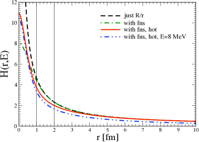
Figure 3: The potential $H_{GT}(r,\bar{E})$. Different approximate forms, as well as the exact one, are shown (color online).

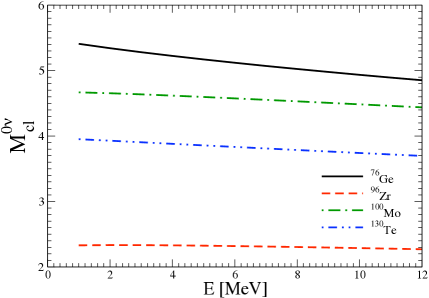
Figure 4: Matrix elements $M^{0\nu}$ for the indicated nuclei evaluated in the closure approximation as a function of the assumed average excitation energy (color online). The values of $M^{0\nu}$ obtained without the closure approximation are 5.24(⁷⁶Ge), 2.62 (⁹⁶Zr), 4.99 (¹⁰⁰Mo), and 4.07 (¹³⁰Te).

II.2 Validity of the closure approximation for the $0\nu\beta\beta$ matrix element

The closure approximation, i.e. the replacement of the summation over the virtual intermediate states by matrix element of a two-body operator, is typically used in the evaluation of the $M^{0\nu}$. It is worthwhile to test the validity of this approximation. Such test can be conveniently performed within the QRPA, where the sum over the intermediate states can be easily carried out. In fact, the calculations performed in Refs. us1 ; us2 ; us3 do not use closure. In this context one can ask two questions: How good is the closure approximation? And what is the value of the corresponding average energy? In Fig. 4 we illustrate the answers to these questions. The exact QRPA matrix elements shown in the caption can be compared with the curves obtained by replacing all intermediate energies with a constant $\bar{E}$, which is varied there between 0 and 12 MeV. One can see, first of all, that the $M^{0\nu}$ changes modestly, by less than 10% when $\bar{E}$ is varied and, at the same time, that the exact results are quite close, but somewhat larger, than the closure ones. Thus, using the closure approximation is appropriate for the evaluation of $M^{0\nu}$ even though it slightly underestimates the $M^{0\nu}$ values. However, the corresponding uncertainty is not more than the other uncertainties involved. We compare the QRPA exact and closure $M^{0\nu}$ for all nuclei of interest in the next section.

III Results and Discussion

We evaluated the nuclear matrix elements (NME) $M^{0\nu}_{GT}$ and $M^{0\nu}$ with and without closure approximation using the Quasiparticle Random Phase Approximation (QRPA).

For all nuclear systems the single-particle model space consisted of $0-5\hbar\omega$ oscillator shells plus $0i_{11/2}$ and $0i_{13/2}$ levels both for protons and neutrons (23 single particle states). The single particle energies were obtained from the Coulomb–corrected Woods–Saxon potential. Two-body interaction G-matrix elements were derived from the Argonne V18 one-boson exchange potential within the Brueckner theory. The pairing interaction was adjusted to fit the empirical pairing gaps cheo93 . The particle-particle and particle-hole channels of the G-matrix interaction of the nuclear Hamiltonian $H$ were renormalized by introducing the parameters $g_{pp}$ and $g_{ph}$, respectively. While $g_{ph}=1.0$ was used throughout, the particle-particle strength parameter $g_{pp}$ was fixed by the data on the two-neutrino double beta decay rates us1 ; us2 ; us3 for each nucleus separately. In the calculation of the $0\nu\beta\beta$-decay NMEs the two-nucleon short-range correlations derived from same potential as residual interactions, namely from the Argonne potential Sim09 , were applied. The unquenched value of the axial current coupling constant, $g_{A}=1.269$ was used here. The modifications caused by the quenching of the weak axial current are discussed in the following two sections.

On the other hand, the absolute values of $M^{2\nu}_{exp}$ were deduced from the averaged values of $2\nu\beta\beta$-decay half-lives of Ref. barab .

In Table 1 we show both the calculated $0\nu\beta\beta$ NMEs evaluated with and without the closure approximation, as well as only the GT parts of their values. Also shown are the experimental $2\nu\beta\beta$-decay NMEs. Using the QRPA method the closure matrix elements $M^{2\nu}_{cl}$ were also evaluated. One can see that the spread among the candidate nuclei of the $2\nu\beta\beta$ NMEs is significatly larger when compared with the spread of the calculated $0\nu\beta\beta$-decay NMEs. The table also demonstrates that using the closure approximation for evaluation of $M^{0\nu}$ makes relatively little difference and that the GT part of $M^{0\nu}$ is dominant in all considered nuclei.

Table 1: The $0\nu\beta\beta$-decay nuclear matrix elements $|M^{0\nu}_{GT}|$ and $|M^{0\nu}|$ calculated within the QRPA. For the parameters used, see the text. The $2\nu\beta\beta$-decay nuclear matrix element $|M^{2\nu}_{exp}|$ were deduced from the avaraged values of the $2\nu\beta\beta$-decay half-lifes barab and $M^{2\nu}_{cl}$ were obtained within the QRPA. For ¹³⁶Xe, where only the upper limit of the $2\nu$ half-life exists, the range shown covers the range of half-lives from the experimental limit to infinity. All entries are evaluated with $g_{A}=1.269$.

NME	${{}^{76}Ge}$	${{}^{82}Se}$	${{}^{96}Zr}$	${{}^{100}Mo}$	${{}^{116}Cd}$	${{}^{128}Te}$	${{}^{130}Te}$	${{}^{136}Xe}$
	$2\nu\beta\beta$-decay NMEs
$|M^{2\nu}_{exp}|~{}[MeV^{-1}]$	0.136	0.095	0.090	0.231	0.126	0.046	0.033	$(0,0.031)$
$M^{2\nu}_{cl}$	0.099	-0.126	-0.802	-0.933	0.059	-0.462	-0.464	(-0.41 -0.25)
	$0\nu\beta\beta$-decay NMEs within closure approximation
$|M^{0\nu}_{GT-cl}|$	4.12	3.61	1.89	3.72	2.77	3.63	3.09	$(1.61,1.83)$
$|M^{0\nu}_{cl}|$	5.02	4.44	2.34	4.59	3.36	4.44	3.79	$(2.00,2.24)$
	$0\nu\beta\beta$-decay NMEs without closure approximation
$|M^{0\nu}_{GT}|$	4.33	3.82	2.16	4.10	2.91	3.92	3.36	$(1.76,1.96)$
$|M^{0\nu}|$	5.24	4.65	2.61	4.99	3.51	4.75	4.07	$(2.15,2.38)$

The values of $M^{0\nu}$ in Table 1 might be compared with the corresponding entries in Table II of Ref. Sim09 . There are small differences between them caused by several changes made in the present work. We use now the updated values of $T^{2\nu}_{1/2}$ of Ref. barab and the more realistic $g_{A}$ = 1.269 instead of 1.25. In evaluating $M^{2\nu}$ we adjust here the energy denominators such that the first $1^{+}$ state has the experimentally known energy value. Moreover, the present results are based on the level scheme with just 23 single particle states, while Ref. Sim09 uses an average of several sets of single particle energies.

Another characteristic feature of the relation between the $M^{0\nu}_{GT}$ and $M^{2\nu}_{cl}$ is illustrated in Fig. 5. There we show the integrals, i.e. the functions of the upper limit of the integration,

$$I^{2\nu}(r_{0})=\int_{0}^{r_{0}}C^{2\nu}_{cl}(r)dr~{},$$

$$I^{0\nu}_{GT}(r_{0})=\int_{0}^{r_{0}}C^{0\nu}_{GT-cl}(r)dr~{}.$$ (16)

Obviously, ${\rm lim}_{r_{0}\rightarrow\infty}I^{2\nu}(r_{0})=M^{2\nu}_{cl}$ and ${\rm lim}_{r_{0}\rightarrow\infty}I^{0\nu}_{GT}(r_{0})=M^{0\nu}_{GT}$.

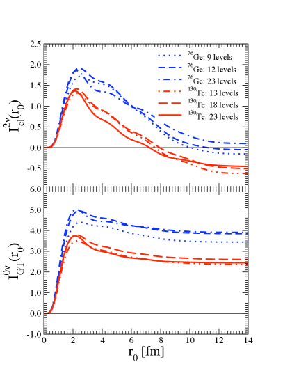
Figure 5: Integrals $I^{2\nu}(r_{0})$ and $I^{0\nu}_{GT}(r_{0})$, Eq.(16), as function of the upper limit $r_{0}$. Three different spaces of single-particle states are considered, small, medium and large (color online).

As one can see the integrals $I^{0\nu}_{GT}(r_{0})$ saturate for $r_{0}\geq 2-3$ fm since the function $C^{0\nu}_{GT}(r)$ is very small past these values of $r$. On the other hand, the functions $I^{2\nu}(r_{0})$ change drastically, even becoming sometimes negative, for $r_{0}\geq 2-3$ fm. That is a reflection of the behavior of the function $C^{2\nu}_{cl}(r)$ that has a substantial tail for $r_{0}\geq 2-3$ fm. In addition, Fig. 5 also demonstrates that the corresponding integrals are almost independent on the number of included single-particle states, as long as at least two full oscillator shells are taken into account.

Remembering that in a nucleus the average distance between nucleons is $\sim$1.2 fm we can somewhat schematically separate the range of the variable $r$ in the functions $C^{0\nu}_{GT}(r)$ and $C^{2\nu}_{cl}(r)$ into the region $r\leq$ 2-3 fm governed by the nucleon-nucleon correlations, while the region $r\geq$ 2-3 fm is governed by nuclear many-body physics. The integrals in Fig. 5 demonstrate that the matrix elements $M^{0\nu}_{GT}$ are almost independent of the “nuclear” region of $r$ and hence one does not expect rapid variations of their value when $A$ or $Z$ of the nucleus is changed. On the other hand, the $2\nu$ closure matrix elements depend sensitively on that region of $r$ and hence one expects sizable shell effects, i.e. a significant variation of $M^{2\nu}$ and $M^{2\nu}_{cl}$ with $A$ and $Z$, in agreement with observations.

IV Quenching of the axial current matrix elements

It is well known that Gamow-Teller $\beta$-decay transitions to individual final states are noticeably weaker than the theory predicts. That phenomenon is known as the axial current matrix elements quenching. The $\beta$-strength functions can be studied also with the charge exchange nuclear reactions and a similar effect is observed as well. Thus, in order to describe the matrix elements of the operator $\sigma\tau$, the empirical rule $(\sigma\tau)^{2}_{eff}\simeq 0.6(\sigma\tau)^{2}_{model}$ is usually used (see Ost92 ; Bro85 ; Cau94 ). Since these operators accompany weak axial current, it is convenient to account for such quenching by using an effective coupling constant $g^{eff}_{A}\sim 1.0$ instead of the true value $g_{A}=1.269$.

The evidence for quenching is restricted so far to the Gamow-Teller operator $\sigma\tau$ and relatively low-lying final states. It is not known whether the other multipole operators associated with the weak axial current should be quenched as well. In fact, the analysis of the muon capture rates in Refs.Kol00 ; Zin06 suggests that quenching is not needed for this process with momentum transfer $q\sim 100$ MeV.

Since the $2\nu\beta\beta$ decay involves only the GT operators and relatively low-lying intermediate states, one could expect that the quenching might be involved in that case. Whether it should be included also for the $0\nu$ mode remains an open question. In the previous paper, Ref. us2 , it was shown that by making the adjustment of the particle-particle coupling strength $g_{pp}$ so that the experimental $2\nu$ halflives are correctly reproduced, the predicted $0\nu$ decay rates are affected by the possible quenching less than the ratio $[(g^{eff}_{A}/g_{A}]^{4}$ might suggest.

Following Ref. us2 we define the “quenched” nuclear matrix elements

$$M^{\prime 0\nu}=\left(\frac{g^{eff}_{A}}{1.269}\right)^{2}M^{0\nu}(g^{eff}_{A})$$ (17)

and use the analogous definitions for $M^{\prime 2\nu}_{cl}$, $M^{\prime 0\nu}_{GT}$ and for the integral $I^{\prime 2\nu}(r_{0})$ and $I^{\prime 0\nu}_{GT}(r_{0})$ see eq. (16).

We use this definition since the experimental quantities, the halflives $T^{0\nu}$ and $T^{2\nu}$, are then simply proportional to $1/M^{\prime 2}$ without the need to modify the phase space factors $G^{2\nu}$ or $G^{0\nu}$ when a different value of $g^{eff}_{A}$ is used. Note that as a consequence of our choice of renormalization of the particle-particle coupling constant $g_{pp}$ the $2\nu\beta\beta$ matrix elements $M^{2\nu}$ by definition become independent of $g^{eff}_{A}$ and thus $M^{2\nu}=M^{\prime 2\nu}$.

In Fig. 6 we show the integrals $I^{\prime 2\nu}_{cl}(r_{0})$ and $I^{\prime 0\nu}_{GT}(r_{0})$ for the case of the decay of ⁷⁶Ge and three values of $(g^{eff}_{A})$. One can see that in the case of $M^{\prime 2\nu}_{cl}$ not only does the final value depend on $(g^{eff}_{A})$, but it affects the dependence on the distance $r_{0}$ as well. With the standard $g_{A}=1.27$ the peak at $r_{0}\sim 2$ fm is compensated by the long tail extending to much larger $r_{0}$, while for the heavily quenched $g^{eff}_{A}=0.8$ the $I^{\prime 2\nu}(r_{0})$ almost saturates at the much smaller values of $r_{0}$. In contrast, the integrals $I^{\prime 0\nu}_{GT}(r_{0})$ saturate at $r_{0}\sim 3$ fm for all considered values of $g^{eff}_{A}$.

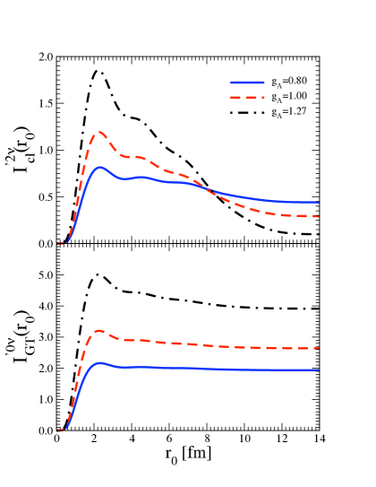
Figure 6: The running sums of $I^{\prime 2\nu}$ (upper panel) and $I^{\prime 0\nu}_{GT}$ (lower panel) for ⁷⁶Ge and different effective values of $g_{A}$. (color online).

It was shown in Ref.us2 that with $g^{eff}_{A}=1.0$ the full matrix elements $M^{\prime 0\nu}$ are reduced by 10-15% compared to their value with $g_{A}=1.25$ used in that paper. Here we use the more correct $g_{A}=1.269$, for adjustment of the particle-particle coupling constant $g_{pp}$ we use the $2\nu$ halflives of Ref. barab that differ slightly from the halflives used in us2 , and the treatment of the short-range correlations is now based on the Ref. Sim09 while in us2 it was based on the phenomenological Jastrow-type function of Ref. Mil76 . In the present work the matrix elements $M^{\prime 0\nu}$ are 20-30% smaller with $g^{eff}_{A}=1.0$ than with $g_{A}=1.269$. Similar effects are also visible in Table II of Ref. Sim09 .

V Determination of the matrix element $M^{2\nu}_{cl}$

While the nuclear matrix elements $M^{2\nu}$ are simply related to the $2\nu$ half-life $T^{2\nu}_{1/2}$, and are therefore known for the nuclei in which $T^{2\nu}_{1/2}$ has been measured, the closure matrix elements $M^{2\nu}_{cl}$ need be determined separately. There are several ways how to accomplish this task:

1. Rely on a nuclear model (e.g. QRPA or nuclear shell model), adjust parameters in such a way that the experimental value of $M^{2\nu}$ is correctly reproduced, and use the model to evaluate $M^{2\nu}_{cl}$. (In QRPA the usual adjustment is the renormalization of the particle-particle coupling constant $g_{pp}$ so that the $T^{2\nu}_{1/2}$ is correctly reproduced.) This procedure is used in Table 1.

2. Use the measured $\beta^{-}$ and $\beta^{+}$ strength functions and assume coherence (i.e. same signs) among states with noticeable strengths in both channels. In this way an upper limit of $M^{2\nu}_{cl}$ can be obtained.

3. Finally, one could invoke the so called “Single state dominance hypothesis” Abad84 according to which the sum in the eqs. (6) and (8) is exhausted by its first term. The measured $\beta$ decay and $EC$ $ft$ values then make it possible to determine both the $M^{2\nu}$ and $M^{2\nu}_{cl}$.

Obviously, none of these methods is exact, but their combination has, perhaps, a chance of constraining the value of $M^{2\nu}_{cl}$ substantially. Examples of application of the latter two items are shown in Table 2. That method can be used, obviously, only for the nuclei where the corresponding experimental data are available.

Table 2: The $2\nu\beta\beta$-decay closure nuclear matrix element $|M^{2\nu}_{cl}|$ evaluated using the Single State Dominance Hypothesis (SSD) and with help of the measured $\beta^{\pm}$ strengths in charge exchange reactions (ChER). The adopted values of the $2\nu\beta\beta$-decay half-times $T^{2\nu-exp}_{1/2}$, taken from Ref. barab are also shown. In the ChER case the matrix elements $|M^{2\nu}|$ and $M^{2\nu}_{cl}$ have been determined by assuming equal phases for its each individual contribution.

		$SSD$			$ChER$
Nucleus	$T^{2\nu-exp}_{1/2}$ [y]		$|M^{2\nu}|$ $[MeV^{-1}]$	$|M^{2\nu}_{cl}|$		$|M^{2\nu}|$ $[MeV^{-1}]$	$|M^{2\nu}_{cl}|$
${}^{48}Ca$	$4.4\times 10^{19}$		-	-		0.083	0.220 Yako
${}^{76}Ge$	$1.5\times 10^{21}$		-	-		0.159	0.522 Grewe
${}^{96}Zr$	$2.3\times 10^{19}$		-	-		-	0.222 Dohmann
${}^{100}Mo$	$7.1\times 10^{18}$		0.208	0.350 Domin		-	-
${}^{116}Cd$	$2.8\times 10^{19}$		0.187	0.349 Domin		0.064	0.305 Rakers
${}^{128}Te$	$1.9\times 10^{24}$		0.019	0.0327 Domin		-	-

Comparison of the NMEs $M^{2\nu}_{exp}$ and $M^{2\nu}_{cl}$ in Table 1 tells us, right away that, at least within the QRPA, the summation in the Eqs. (6) and (8) contains both positive and negative parts (see also Fig. 5). This is obviously so since for most nuclei the quantity $\bar{E}_{2\nu}-(M_{i}+M_{f})/2$ in Eq. (8) becomes negative, while each of the denominators in the Eq. (6) is positive. Hence, we cannot expect good agreement between the $M^{2\nu}_{cl}$ from QRPA and those from the items 2. and 3. above. And, moreover, we cannot expect that SSD is a valid hypothesis for all candidate nuclei. Comparison of the corresponding entries in Tables 1 and 2 confirms that expectation.

Since there is a substantial experimental activity devoted to the determination of the $\beta^{\pm}$ strengths, it is worthwhile to examine in more detail the somewhat unexpected finding that in many cases $M^{2\nu}$ and $M^{2\nu}_{cl}$ have opposite signs. Obviously, this has to do with the different weight of the corresponding terms in the Eqs. (6) and (8). We plot in Fig. 7 the corresponding running sums as a function of the excitation energy in the intermediate nucleus. One can see that the negative values of $M^{2\nu}_{cl}$ arise from excitation energies $E_{ex}>10$ MeV that are difficult to explore experimentally.

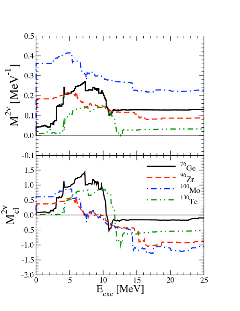
Figure 7: The running sums of $M^{2\nu}$ (upper panel) and $M^{2\nu}_{cl}$ (lower panel) for selected nuclei. (color online). $g_{A}=1.269$ was used.

The negative contributions to $M^{2\nu}$ and $M^{2\nu}_{cl}$ from higher excitation energies cause in several nuclei even the reversal of the sign of $M^{2\nu}_{cl}$ to the negative one. While, clearly, there is a substantial $\beta^{-}$ strength at these excitation energies, QRPA predicts that there is a sufficient $\beta^{+}$ strength there as well, leading to the reduction of the $M^{2\nu}$ and $M^{2\nu}_{cl}$ visible in Fig. 7. Our QRPA calculations suggest that about 0.2 units of the B(GT) $\beta^{+}$ strength is distributed among states with $E_{ex}\geq 10$ MeV in all considered nuclei. Such $\beta^{+}$ strength has not been observed experimentally so far. It remains to be seen whether it exists at all, or is hidden in the “grass”, i.e. distributed among many weak states that escape identification. Until this dilemma is resolved we cannot decide whether the closure matrix elements $M^{2\nu}_{cl}$ in Table I are realistic or not.

In the previous section we discussed the phenomenon of quenching of the axial current matrix elements. Fig. 6 suggests that using the effective $g^{eff}_{A}<1.27$ reduces the negative contribution of the higher lying $1^{+}$ states to the matrix element $M^{\prime 2\nu}_{cl}$. To see how large that effect might be we performed QRPA calculation with $g^{eff}_{A}=0.9$ based on the empirical evidence that the degree of quenching increases with $A$. The resulting quenched matrix elements $M^{\prime 2\nu}_{cl}$ are shown in Table 3. While, as remarked earlier, it is unknown whether all mutipoles are affected by the axial current quenching, not only the GT $1^{+}$ states, we nevertheless show in the same Table the values of quenched $M^{\prime 0\nu}_{GT}$ and of the full NME $M^{\prime 0\nu}$ with and without the closure approximation. If quenching would not affect these matrix elements, their magnitude would be enhanced by the factor $(1.269/0.9)^{2}\sim 2$ making them substantially larger than the values in Table 1.

Table 3: The experimental values $M^{\prime 2\nu}_{exp}$ and the QRPA values of $M^{\prime 2\nu}_{cl}$ evaluated with quenching at $g_{A}=0.9$. The corresponding quenched values of the $0\nu\beta\beta$ matrix elements are also shown.

NME	${{}^{76}Ge}$	${{}^{82}Se}$	${{}^{96}Zr}$	${{}^{100}Mo}$	${{}^{116}Cd}$	${{}^{128}Te}$	${{}^{130}Te}$	${{}^{136}Xe}$
	$2\nu\beta\beta$-decay NMEs
$|M^{\prime 2\nu}_{exp}|~{}[MeV^{-1}]$	0.136	0.095	0.090	0.231	0.126	0.046	0.033	$(0,0.031)$
$M^{\prime 2\nu}_{cl}$	0.336	0.100	-0.210	-0.205	0.179	-0.146	-0.169	(-0.25, -0.047)
	$0\nu\beta\beta$-decay quenched NMEs within closure approximation
$M^{\prime 0\nu}_{GT-cl}$	2.50	2.10	1.20	2.23	1.63	2.09	1.77	(0.86, 1.08)
$M^{\prime 0\nu}_{cl}$	3.82	3.25	1.91	3.49	2.45	3.28	2.82	(1.43, 1.72)
	$0\nu\beta\beta$-decay quenched NMEs without closure approximation
$M^{\prime 0\nu}_{GT}$	2.59	2.20	1.33	2.45	1.71	2.23	1.91	(0.93, 1.14)
$M^{\prime 0\nu}$	3.90	3.34	2.05	3.71	2.53	3.44	2.96	(1.51, 1.78)

Since our goal is the determination of the GT part of the $0\nu\beta\beta$ matrix element $M^{0\nu}_{GT}$, a priori the knowledge of the $M^{2\nu}_{cl}$, which depends only on the $1^{+}$ intermediate states, is insufficient. According to the Eq. (13) we need for that purpose the function $C^{2\nu}_{cl}(r)$ that depends, in principle, on all intermediate multipoles. However, is we could use the expansion of the spherical Bessel function $j_{0}(qr)$ in Eq.(14) in powers of $qr$ and keep just the first term, the neutrino potential $H(r,\bar{E})$ would be represented by a constant and the Eq.(13) would predict a simple proportionality between $M^{2\nu}_{cl}$ and $M^{0\nu}_{GT}$. However, such an expansion does not work. In reality in Eq. (14) $qr\geq 1$ and we cannot approximate the neutrino potential $H(r,\bar{E})$ by its value at $r=0$. Hence, we do not expect a proportionality between $M^{2\nu}_{cl}$ and $M^{0\nu}_{GT}$ and the QRPA evaluation supports this conclusion.

VI Conclusions

Since the nuclear matrix elements $M^{0\nu}$ must be determined theoretically, it is of obvious interest to search for any relation between their numerical values and other quantities that are either known from experiments or at least constrained by them. Here we describe such a relation between the dominant Gamow-Teller part $M^{0\nu}_{GT}$ of $M^{0\nu}$ and the matrix element $M^{2\nu}_{cl}$ of the observed $2\nu\beta\beta$-decay evaluated in the closure approximation. The relation is based on the evaluation of the auxiliary functions $C^{0\nu}_{GT}(r)$ and $C^{2\nu}_{cl}(r)$ that describe the dependence of the corresponding nuclear matrix elements on the distance $r$ between the pair of neutrons that is transformed in the $\beta\beta$ decay into a pair of protons. Thus (see Eqs. (5), (8) and (13))

$$M^{0\nu}_{GT}=\int_{0}^{\infty}C^{0\nu}_{GT}(r)dr~{},~{}M^{2\nu}_{cl}=\int_{0}^{\infty}C^{2\nu}_{cl}(r)dr~{},$$

$${\rm and}~{}C^{0\nu}_{GT}(r)=H(r,\bar{E})\times C^{2\nu}_{cl}(r)~{},$$ (18)

represents the required relation.

However, while the matrix elements $M^{2\nu}$ and $M^{2\nu}_{cl}$ depend only on the transition strengths and energies of the $1^{+}$ virtual intermediate states (they are pure $GT$ quantities), the function $C^{2\nu}_{cl}(r)$ gets contribution from all multipoles. Thus, the relation that we found is an indirect one; even if $M^{2\nu}_{cl}$ would be precisely known, the evaluation of the function $C^{2\nu}_{cl}(r)$ requires additional nuclear theory input.

Nevertheless, the relation in Eq. (13) allows us to obtain a better insight into the problem of the $A$ and $Z$ dependence of the matrix elements $M^{2\nu}$ and $M^{0\nu}$. While the known $M^{2\nu}$ have a strong shell dependence, the calculated $M^{0\nu}$ vary much less. Analysis of the functions $C^{2\nu}_{cl}(r)$ and $C^{o\nu}_{GT}(r)$ makes it possible to better understand where this fundamental difference comes from.

We show that, so far, the QRPA values of closure approximation $M^{2\nu}_{cl}$ matrix elements do not agree well with the same quantities based on the measured $\beta^{-}$ and $\beta^{+}$ strength functions and on the assumption of coherence (i.e. same sign) of contributions of individual states. Until this discrepancy is resolved, it is difficult to employ $M^{2\nu}_{cl}$ in order to constrain the magnitude of the $0\nu\beta\beta$ matrix elements $M^{0\nu}_{GT}$.

References

- (1) F. T. Avignone, S. R. Elliott and J. Engel, Rev. Mod. Phys. 8 0, 481 (2008).
- (2) V. A. Rodin, A. Faessler, F. Šimkovic and P. Vogel, Phys. Rev. C68, 044302(2003).
- (3) V. A. Rodin, A. Faessler, F. Šimkovic and P. Vogel, Nucl. Phys. A766, 107 (2006), and erratum A793, 213 (2007).
- (4) F. Šimkovic, A. Faessler, V. A. Rodin, P. Vogel, and J. Engel, Phys. Rev. C bf 77, 045503(2008).
- (5) J. Suhonen, Phys. Lett. B607, 87 (2005); J. Suhonen and O. Civitarese, Phys. Lett. B626, 80 (2005); ibid Nucl. Phys. A761, 313 (2005).
- (6) H. Primakoff and S. P. Rosen, Rep. Prog. Phys. 22, 121 (1959).
- (7) J. Menendez, A. Poves, E. Caurier and F. Nowacki, Nucl. Phys. A818, 139 (2009).
- (8) E. Caurier, J. Menendez, F. Nowacki, and A. Poves, Phys. Rev. Lett. 100 052503 (2008).
- (9) E. Caurier, F. Nowacki, and A. Poves, Eur. J. Phys. A36, 195 (2008).
- (10) J. Barea and F. Iachello, Phys. Rev. C79, 054302 (2009).
- (11) B. Pontecorvo, Phys. Lett. B26, 630 (1968).
- (12) J. Engel and P. Vogel, Phys. Rev. C69, 034304 (2004).
- (13) I.S. Towner and J.C. Hardy, in Symmetries and Fundamental Interactions in Nuclei, W.C. Haxton and E.M. Henley eds, nucl-th/9504015.
- (14) F. Šimkovic, G. Pantis, J. D. Vergados, and A. Faessler, Phys. Rev. C60, 055502 (1999).
- (15) F. Šimkovic, A. Faessler, H. Müther, V. Rodin, and M. Stauf, Phys. Rev. C79, 055501 (2009).
- (16) M.K. Cheoun, A. Bobyk, A. Faessler, F. Šimkovic and G. Teneva, Nucl. Phys. A 561, 74 (1993).
- (17) A.S. Barabash, Phys. Rev. C81, 035501 (2010).
- (18) F. Osterfeld, Rev. Mod. Phys. 64, 491 (1992).
- (19) B. A. Brown and G. H. Wildenthal, ATNDT 33, 347 (1985).
- (20) E. Caurier, A. P. Zuker, A. Poves and G. Martinez-Pinedo, Phys. Rev. C50, 225 (1994).
- (21) E. Kolbe, K. Langanke and P. Vogel, Phys. Rev. C62, 055502(2000).
- (22) N. T. Zinner, K. Langanke and P. Vogel, Phys. Rev. C74, 024326 (2006).
- (23) G. A. Miller and J. E. Spencer, Ann. Phys. 100, 562 (1976).
- (24) J. Abad, A. Morales, R. Nunez-Lagos, and A. Pacheco, Ann. Fiz. A80, 9 (1984).
- (25) K. Yako et al., Phys. Rev. Lett. 103, 012503 (2009).
- (26) E.-W. Grewe et al., Phys. Rev. C 78, 044301 (2008).
- (27) H. Dohmann et al., Phys. Rev. C 78, 041602R (2008).
- (28) S.Rakers et al., Phys. Rev. C 71, 054313 (2005).
- (29) P.Domin et al., Nucl. Phys. A 753, 337 (2005).