Associated production of one particle and a Drell-Yan pair in hadronic collisions

Abstract

We propose a collinear factorization formula for the associated production of one particle and a Drell-Yan pair in hadronic collisions. It is shown that additional collinear singularities appearing in the next-to-leading order calculations that can not be factorized into parton and fragmentation functions are systematically renormalized by introducing fracture functions. Next-to-leading order coefficient functions for cross-sections double differential in the fractional energy of the identified hadron and lepton pair invariant mass are presented.

I Introduction

The description of particle production in hadronic collisions is interesting and challenging in many aspects. Perturbation theory can be applied whenever a sufficiently hard scale characterizes the scattering process. The comparison of early LHC charged particle spectra with next-to-leading order perturbative QCD predictions stratmann shows that the theory offers a rather good description of data at sufficiently high hadronic transverse momentum, of the order of a few GeV. For inelastic scattering processes at even lower transverse momentum, the theoretical description in terms of perturbative QCD breaks down since both the coupling and partonic matrix elements diverge as the transverse momenta of final state parton vanish. In this paper we will study the semi-inclusive version of the Drell-Yan process, $H_{1}+H_{2}\rightarrow H+\gamma^{*}+X$, in which one particle is tagged in the final state together with the Drell-Yan pair. In such a process the high invariant mass of the lepton pair, $Q^{2}$, constitutes the perturbative trigger which guarantees the applicability of perturbative QCD. The detected hadron $H$ could then be used, without any phase space restriction, as a local probe to investigate particle production mechanisms. The evaluation of $\mathcal{O}(\alpha_{s})$ corrections shows that there exists a class of collinear singularities escaping the usual renormalization procedure which amounts to reabsorb collinear divergences into a redefinition of bare parton and fragmentation functions. Such singularities are likely to appear in every fixed order calculation in the same kinematical limits spoiling the convergence of the perturbative series. We therefore show how to improve the theoretical description providing a generalized procedure for the factorization of such additional collinear singularities. Most important, the latter is the same as the one proposed in Deep Inelastic Scattering Graudenz where the same collinear singularities pattern is also found, confirming the universality of the collinear radiation between different hard processes. The latter will make use the concept of fracture functions and the renormalization group equations associated with them Trentadue_Veneziano . In a pure parton model approach, these non-perturbative distributions effectively describe the hadronization of the spectators system in hadron-induced reactions. We will demonstrate that the transverse-momentum integrated cross-section is finite and valid for all transverse momentum of the detected hadron, without any restriction imposed by the singular behaviour of matrix elements. We further note that this process is the single-particle counterpart of electroweak-boson plus jets associated production zjets , presently calculated at nex-to-leading order accuracy with up to three jets in the final state w3jet . One virtue of jet requirement is that it indeed avoids the introduction of fragmentation functions to model the final state, which are instead one of the basic ingredients entering our formalism. At variance with our case, however, jet reconstructions at very low transverse momentum starts to be challenging cacciari and it makes difficult the study of this interesting portion of the produced particle spectrum.

In Ref. newfracture a first attempt was made to study the associated radiation in Drell-Yan type process with the aid of the concept of extended fracture functions extendedM . The collinear factorization formula was then studied in Ref. SIDYmy where we were mainly concerned with the study of hard diffractive processes in hadronic collisions. The latter are a special case of associated production in which the tagged hadron is a proton at very low transverse momentum and almost the energy of the incoming proton. In this paper we consider the production of a generic hadron and report all the coefficient functions for the cross-sections differential in the invariant mass of the lepton pair and fractional momentum of the detected hadron.

The outline of this paper is as follows. In Section II we set the notation and briefly review the factorization of collinear singularities in the inclusive Drell-Yan process. In Section III we evaluate the $\mathcal{O}(\alpha_{s})$ contributions to the cross-section in which the hadron is produced by the fragmentation of a final state parton. In Section IV we define the parton model cross-section for the associated production of one particle and a Drell-Yan pair in term of fracture functions and evaluate the corresponding $\mathcal{O}(\alpha_{s})$ corrections. In Section V we present the finite cross sections in terms of renormalized fracture functions, distribution functions and fragmentation functions. The paper closes with a summary and some conclusions. Technical details and explicit formulas are collected in the appendix.

II Inclusive Drell-Yan process

In this section we briefly review the factorization of collinear singularities for the inclusive Drell-Yan process, which will be then properly generalized when dealing with the associated production case. Consider therefore the collision of two hadrons $H_{1}$ and $H_{2}$ of momenta $P_{1}$ and $P_{2}$, respectively:

$$H_{1}(P_{1})+H_{2}(P_{2})\rightarrow\gamma^{*}(q)+X\,,$$ (1)

where $\gamma^{*}$ stands for the virtual photon of invariant mass $Q^{2}\gg\Lambda_{QCD}^{2}$ and $X$ for the unobserved part of the final state. The dilepton pair detected in the final state is the decay product of a virtual photon $\gamma^{*}$ created, to lowest order, by the annihilation of a quark and an antiquark with momenta $p_{1}=x_{1}P_{1}$ and $p_{2}=x_{2}P_{2}$, respectively, and both assumed to be collinear to their parent hadron. The corresponding differential cross-section threfore is given by DY

$$\frac{d\sigma(\tau)}{dQ^{2}}=\sigma_{0}\int_{\tau}^{1}\frac{dx_{1}}{x_{1}}\int^{1}_{\frac{\tau}{x_{1}}}\frac{dx_{2}}{x_{2}}\sum_{q}e_{q}^{2}\Big{[}f_{q}^{[1]}(x_{1})f_{\bar{q}}^{[2]}(x_{2})+(q\leftrightarrow\bar{q})\Big{]}\delta(1-w)\,.$$ (2)

The puntiform cross-section is denoted by $\sigma_{0}=4\pi\alpha^{2}_{\makebox{\tiny{em}}}/9S_{h}Q^{2}$. The hadronic centre of mass energy is denoted by $S_{h}=(P_{1}+P_{2})^{2}$ and the relevant ratio $\tau$ is defined by $\tau=Q^{2}/S_{h}$. To zeroth order in $\alpha_{s}$, the partonic sub-process squared energy $\hat{s}=(p_{1}+p_{2})^{2}$ is fixed to be $s=x_{1}x_{2}S_{h}=Q^{2}$, from which the constraint $w=\tau/x_{1}x_{2}=1$ follows. The flavour sum runs on quarks only. The puntiform cross-sections $\sigma_{0}$ is weighted by the convolution over parton distributions, $f_{q}^{[1]}$ and $f_{\bar{q}}^{[2]}$, evaluated at fractional momenta $x_{1}$ and $x_{2}$. The integration limits are fixed by momentum conservation. We further assign to each parton distribution function an index $n=[1,2]$ denoting the hadron from which the quark (or antiquark) has been extracted. Calculations are performed in dimensional regularization with space-time dimension set to $n=4-2\epsilon$. Following Ref. DYNLO , the cross-section for the partonic sub-process $q(p_{1})+\bar{q}(p_{2})\rightarrow\gamma^{*}(q)$ is given by

$$\frac{d\sigma_{q\bar{q}}(w,Q^{2})}{dQ^{2}}=\delta(1-w)\,.$$ (3)

It defines the normalization of the partonic Drell Yan cross section and corresponds to multiplying all matrix elements by a factor $2N_{c}/(1-\epsilon)$, $N_{c}$ being the number of colours. The latter factor is already absorbed in the puntiform cross-section $\sigma_{0}$ in parton model formula, eq. (2). The evaluation on next-to-leading corrections is performed by computing the relavant real emissions and virtual diagrams. We refer to reader to Ref. DYNLO for the explicit expressions of matrix elements and further calculational details. Both real and virtual terms develop poles in $\epsilon^{-2}$ which mutually cancel when these contributions are added so that one finally obtains

$$\frac{d\sigma(\tau)}{dQ^{2}}=\sigma_{0}\int_{\tau}^{1}\frac{dx_{1}}{x_{1}}\int_{\frac{\tau}{x_{1}}}^{1}\frac{dx_{2}}{x_{2}}\sum_{q}e_{q}^{2}\Bigg{\{}$$ (4)

$$\Big{[}f_{q}^{[1]}(x_{1})f_{\bar{q}}^{[2]}(x_{2})+(q\leftrightarrow\bar{q})\Big{]}\Big{[}\delta(1-w)-\frac{2}{\epsilon}\frac{\alpha_{s}}{2\pi}P_{qq}(w)\,c_{0}+\frac{\alpha_{s}}{2\pi}\widetilde{C}_{q\bar{q}}(w)\Big{]}+$$

$$\hskip 99.58464pt+\Big{[}\big{(}f_{g}^{[1]}(x_{1})f_{\bar{q}}^{[2]}(x_{2})+f_{q}^{[1]}(x_{1})f_{g}^{[2]}(x_{2})\big{)}+(q\leftrightarrow\bar{q})\Big{]}\cdot$$

$$\hskip 199.16928pt\cdot\Big{[}-\frac{1}{\epsilon}\frac{\alpha_{s}}{2\pi}P_{qg}(w)\,c_{0}+\frac{\alpha_{s}}{2\pi}\widetilde{C}_{qg}(w)\Big{]}\Bigg{\}}\,.$$

In the previous equation collinear singularities appear as poles in $\epsilon^{-1}$ multiplying the leading order DGLAP splitting functions $P_{ij}(w)$. The adimensional factor $c_{0}$ appearing in eq. (4) reads

$$c_{0}=\Big{(}\frac{4\pi\mu_{R}^{2}}{Q^{2}}\Big{)}^{\epsilon}\frac{\Gamma(1-\epsilon)}{\Gamma(1-2\epsilon)}\,$$ (5)

where $\mu_{R}^{2}$ indicates the renormalization scale. The subtraction of singular terms in the partonic cross-sections is performed by absorbing the collinear divergences into bare parton distributions, which in the $\overline{\mbox{MS}}$ scheme amounts to the following redefinition:

$$f_{i}(x)=\int_{x}^{1}\frac{du}{u}\Big{[}\delta_{ij}\delta(1-u)+\frac{1}{\epsilon}\frac{\alpha_{s}}{2\pi}\frac{\Gamma(1-\epsilon)}{\Gamma(1-2\epsilon)}\Big{(}\frac{4\pi\mu_{R}^{2}}{\mu_{F}^{2}}\Big{)}^{\epsilon}P_{ij}(u)\Big{]}f_{j}\Big{(}\frac{x}{u},\mu_{F}^{2}\Big{)}\,.$$ (6)

The renormalized distributions do depend on the scale, $\mu_{F}^{2}$, at which the factorization is performed, and their variation with respect to it gives governed by DGLAP evolution equations DGLAP . Inserting eq. (6) into eq. (4) one can explicitely check that collinear singularities, proportional to poles in $\epsilon$, do cancel. The finite result reads:

$$\frac{d\sigma(\tau)}{dQ^{2}}=\sigma_{0}\int_{\tau}^{1}\frac{dx_{1}}{x_{1}}\int_{\frac{\tau}{x_{1}}}^{1}\frac{dx_{2}}{x_{2}}\sum_{q}e_{q}^{2}\Bigg{\{}$$ (7)

$$\Big{[}f_{q}^{[1]}(x_{1},\mu_{F}^{2})f_{\bar{q}}^{[2]}(x_{2},\mu_{F}^{2})+(q\leftrightarrow\bar{q})\Big{]}\Big{[}\delta(1-w)+\frac{\alpha_{s}}{2\pi}C_{q\bar{q}}(w,\mu_{F}^{2}/Q^{2})\Big{]}+$$

$$\Big{[}\big{(}f_{g}^{[1]}(x_{1},\mu_{F}^{2})f_{\bar{q}}^{[2]}(x_{2},\mu_{F}^{2})+f_{q}^{[1]}(x_{1},\mu_{F}^{2})f_{g}^{[2]}(x_{2},\mu_{F}^{2})\big{)}+(q\leftrightarrow\bar{q})\Big{]}\frac{\alpha_{s}}{2\pi}C_{qg}(w,\mu_{F}^{2}/Q^{2})\Bigg{\}}\,.$$

The infrared-finite coefficient functions $\widetilde{C}_{ij}(w)$ and $C_{ij}(w)$, defined in the $\overline{\mbox{MS}}$ scheme, are reported in appendix A. In phenomenological applications it is costumary to set $\mu_{F}^{2}=Q^{2}$ in eq. (7). This choice removes large logarithms of the ratio $\mu_{F}^{2}/Q^{2}$ appearing in the coefficient functions. At the same time, the evaluation of parton distributions at a scale $\mu_{F}^{2}=Q^{2}$ accounts for the resummation of such logarithms via DGLAP evolution equations.

III Associated production

In the present and next section we consider the next-to-simple generalization of reaction in eq. (1), namely the associated production of a Drell-Yan pair and an identified hadron $H$ of momentum $h$:

$$H_{1}(P_{1})+H_{2}(P_{2})\rightarrow\gamma^{*}(q)+H(h)+X\,.$$ (8)

In particular we will evaluate $\mathcal{O}(\alpha_{s})$ corrections to the cross-section double differential in the invariant mass $Q^{2}$ of the lepton pair and the fractional energy of the identified hadron $H$, defined in analogy with $e^{+}e^{-}$ annihilation process:

$$z=\frac{2h\cdot(P_{1}+P_{2})}{(P_{1}+P_{2})^{2}}=\frac{2E_{H}}{\sqrt{S_{h}}}\,.$$ (9)

The last equality in the previous equations holds in the hadronic centre of mass frame. In this frame $z$ is the proportional to the detected hadron energy, $E_{H}$, scaled down by the beam energy, $\sqrt{S_{h}}/2$. In this section we consider the $\mathcal{O}(\alpha_{s})$ production mechanism in which the observed hadron $H$ is given by the fragmentation of a, real, final state parton and address such contribution as central. We label the momenta in the partonic sub-process as $i(p_{1})+j(p_{2})\rightarrow l(k)+\gamma^{*}(q)$, where $k$ and $q$ are the four-momenta of the outgoing parton and virtual photon, respectively. In general such a correction is expected in the form aversa

$$\frac{d\sigma^{C}(\tau,z,Q^{2})}{dQ^{2}dz}\propto\sum_{ijl}\int\frac{dx_{1}}{x_{1}}\int\frac{dx_{2}}{x_{2}}\int\frac{d\rho}{\rho}f_{i}(x_{1})f_{j}(x_{2})D_{l}^{H}(z/\rho)\frac{d\hat{\sigma}^{ij\rightarrow l\gamma^{*}}}{dQ^{2}d\rho}\,,$$ (10)

where $\rho=2E_{l}/\sqrt{S_{h}}$ is the fractional energy of the outgoing parton evaluated in the hadronic center of mass frame and it is the partonic analogue of the hadronic $z$. The sum runs over all possible partonic sub-processes

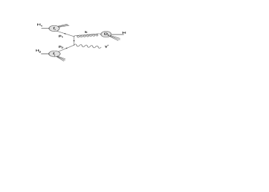
Figure 1: One of the diagrams contributing to eq. (10). The observed hadron $H$ is produced by the fragmentation of the final state parton $l$.

and the partonic cross-sections are indicated with $d\hat{\sigma}^{ij\rightarrow l\gamma^{*}}$. With respect to eq. (2), eq. (10) does contain an additional convolution on the fractional energy $\rho$ of the final state parton weighted by the fragmentation functions $D_{l}^{H}$. The latter gives the probability that a parton with fractional energy $\rho$ fragments into the observed hadron $H$ with fractional energy $z$. One of the diagrams contributing to eq. (10) is depicted in Fig. (1). We found useful to rewrite the convolution formula as a function of $y=(1-\cos\theta)/2$, where $\theta$ is its angle between the parton $l$ and the hadron $H_{1}$ in the hadronic center of mass frame. Within these definitions the parton-level invariants $\hat{u}$ and $\hat{t}$ in the matrix elements can be rewritten in this frame as

$$\hat{t}\;=\;(p_{1}-k)^{2} = -\;\hat{s}\,(1-w)\;\frac{x_{1}\,y}{x_{1}y+x_{2}(1-y)}\,,$$ (11)

$$\hat{u}\;=\;(p_{2}-k)^{2} = -\;\hat{s}\,(1-w)\;\frac{x_{2}\,(1-y)}{x_{1}y+x_{2}(1-y)}\,,$$

where $\hat{s}=(p_{1}+p_{2})^{2}$ and $w=\tau/(x_{1}x_{2})$. The phase space reads:

$$dPS^{(2)}=\frac{1}{8\pi}\Big{(}\frac{4\pi}{Q^{2}}\Big{)}^{\epsilon}\;\big{(}x_{1}x_{2}-\tau\big{)}^{1-2\epsilon}\;\big{(}x_{1}y+x_{2}(1-y)\big{)}^{2\epsilon-2}\;\frac{\tau^{\epsilon}}{\Gamma(1-\epsilon)}\;dy\;y^{-\epsilon}\;(1-y)^{-\epsilon}\,.$$ (12)

The angular variable $y$ and the fractional energy $\rho$ of the emitted parton are not independent and constrained by:

$$\rho(y)=\frac{x_{1}x_{2}-\tau}{x_{1}y+x_{2}(1-y)}\,.$$ (13)

The available phase space must take into account that there should be enough energy for the production both of the hadron $H$ and the virtual photon $\gamma^{*}$. This phase space constraints will appear in the convolution limits in eq. (10). In order to obtain them, we notice that the parent parton of the observed hadron is required to have a fractional energy $\rho\geq z>0$. Applying this last constraint to eq. (13), one is able to determine the boundaries $r_{1}$ and $r_{2}$ in the $x_{1}$ and $x_{2}$ convolutions integrals. They are both $z$ and $y$ dependent and read

$$r_{1}(\tau,z;y)=\frac{\tau+z(1-y)}{1-zy}\,,$$

$$r_{2}(\tau,z;y)=\frac{\tau+x_{1}zy}{x_{1}-z(1-y)}\,.$$ (14)

The $\mathcal{O}(\alpha_{s})$ corrections in the central region therefore reads

$$\frac{d\sigma^{C}(\tau)}{dQ^{2}dz}=\sigma_{0}\int_{0}^{1}dy\int_{r_{1}}^{1}\frac{dx_{1}}{x_{1}}\int_{r_{2}}^{1}\frac{dx_{2}}{x_{2}}\sum_{q}e_{q}^{2}\Big{\{}$$ (15)

$$\Big{[}f_{q}^{[1]}(x_{1})\,f_{\bar{q}}^{[2]}(x_{2})+(q\leftrightarrow\bar{q})\Big{]}\,D_{g}^{H}(z/\rho)\Big{[}-\frac{1}{\rho}\frac{\alpha_{s}}{2\pi}\frac{c_{0}}{\epsilon}\widehat{P}_{qq}(w)[\delta(y)+\delta(1-y)]+\frac{\alpha_{s}}{2\pi}\widetilde{K}_{q\bar{q}}(y)\Big{]}+$$

$$f_{g}^{[1]}(x_{1})\Big{[}f_{\bar{q}}^{[2]}(x_{2})D_{\bar{q}}^{H}(z/\rho)+(q\leftrightarrow\bar{q})\Big{]}\Big{[}-\frac{1}{\rho}\frac{\alpha_{s}}{2\pi}\frac{c_{0}}{\epsilon}\widehat{P}_{qg}(w)\delta(y)+\frac{\alpha_{s}}{2\pi}\widetilde{K}_{qg}(y)\Big{]}+$$

$$f_{g}^{[2]}(x_{2})\Big{[}f_{\bar{q}}^{[1]}(x_{1})D_{\bar{q}}^{H}(z/\rho)+(q\leftrightarrow\bar{q})\Big{]}\Big{[}-\frac{1}{\rho}\frac{\alpha_{s}}{2\pi}\frac{c_{0}}{\epsilon}\widehat{P}_{qg}(w)\delta(1-y)+\frac{\alpha_{s}}{2\pi}\widetilde{K}_{qg}(1-y)\Big{]}\Big{\}}\,,$$

where $\rho=\rho(y)$ via eq. (13) and we used the shorthand $\widetilde{K}_{ij}(y)$ for $\widetilde{K}_{ij}(y,x_{1},x_{2},w)$. The expressions for infrared finite coefficients $\widetilde{K}_{ij}$ are collected in appendix A. Eq. (15) displays two disjoint singular limits for $y\rightarrow 0$ and $y\rightarrow 1$. In order to expose the collinear singularites we have performed an $\epsilon$-expansion on the angular variable $y$:

$$(1-y)^{-1-\epsilon} \simeq -\frac{1}{\epsilon}\,\delta(1-y)+\Big{(}\frac{1}{1-y}\Big{)}_{+[0,\underline{1}]}-\epsilon\Big{(}\frac{\ln(1-y)}{1-y}\Big{)}_{+[0,\underline{1}]}+\mathcal{O}(\epsilon^{2})\,,$$ (16)

$$y^{-1-\epsilon} \simeq -\frac{1}{\epsilon}\,\delta(y)+\Big{(}\frac{1}{y}\Big{)}_{+[\underline{0},1]}-\epsilon\Big{(}\frac{\ln y}{y}\Big{)}_{+[\underline{0},1]}+\mathcal{O}(\epsilon^{2})\,.$$ (17)

The unregularized splitting functions $\widehat{P}_{ij}$ appearing in eq. (15) are given by KUV

$$\widehat{P}_{qq}(w)=C_{F}\frac{1+w^{2}}{1-w},\;\;\;\widehat{P}_{qg}(w)=T_{R}[w^{2}+(1-w)^{2}]\,,$$ (18)

with $C_{F}=4/3$ and $T_{R}=1/2$. We wish to conclude this section by noting that the collinear divergences appearing in eq. (15) do correspond to configurations in which the parent parton of the observed hadron is collinear to the incoming parton. Such divergences at vaninishing transverse momentum escape, as shown already in the context of Semi-Inclusive Deep Inelastic Scattering Graudenz , any factorization in terms of renormalized parton distributions and fragmentation functions. While for many practical applications they are regularized introducing an arbitrary cut-off on the produced hadron transverse momentum, configurations which give rise to these divergences will be present at every order in perturbative calculations. Fracture functions together with their own renormalization group equations can be shown to provide the correct tool to perform the resummation to all orders of large logarithmic contributions coming from the factorization of such collinear singularities.

IV Corrections in the target region

To lowest order in the QCD coupling no hadron can be produced in the final state since QCD radiation is absent. In this case we assume that hadron production is described by fracture functions $M^{H/H_{1}}_{i}(x_{1},z)$ and $M^{H/H_{2}}_{j}(x_{2},z)$. These non-perturbative distributions give the conditional probability of finding a parton $i$($j$) of fractional momemntum $x_{1}$($x_{2}$) in the incoming hadron $H_{1}$($H_{2}$) while an hadron $H$, with fractional momentum $z$, is detected in the final state Trentadue_Veneziano . In a pure parton model approach they describe hadron production in the target fragmentation region of $H_{1}$ or $H_{2}$. The latter regions, denoted by $\mathcal{R}_{T_{1}}$ and $\mathcal{R}_{T_{2}}$, respectively, can be defined as $\theta=0$ and $\theta=\pi$, where $\theta$ is the angle between $H$ and $H_{1}$ defined in the centre of mass frame. Fracture function were originally introduced to describe hadron production in the Deep Inelastic Scattering target fragmentation region. A renormalization group evolution equations were derivered Trentadue_Veneziano with the aid of Jet Calculus technique KUV . Subsequently the soft and collinear factorization of these distributions in Semi-Inclusive DIS was proven respectively in Refs. Fact_M_soft ; Fact_M_coll . A complete one loop calculation was presented in Ref. Graudenz , confirming the factorization conjecture first formulated in Ref. Trentadue_Veneziano . We emphasize that by virtue of the factorization theorem, fracture functions are univeral distributions, at least in the context of Semi-Inclusive DIS. In hadronic collisions however such a proof does not exist and counter example to it have been given in the context of diffractive production in Ref. Fact_M_soft . The main motivation for using fracture functions in the present context is that, as we shall prove in the following sections, they allow us to systematically factorize collinear divergences occuring in the evaluation of the partonic cross-sections. Given these assumptions, we now present the parton-model formula, depicted in Fig. (2), for the associated production case:

$$\frac{d\sigma^{H}(\tau)}{dQ^{2}dz}=$$ (19)

$$\sigma_{0}\int_{\tau}^{1-z}\frac{dx_{1}}{x_{1}}\int_{\frac{\tau}{x_{1}}}^{1}\frac{dx_{2}}{x_{2}}\sum_{q}e_{q}^{2}\Big{[}M_{q}^{[1]}(x_{1},z)f_{\bar{q}}^{[2]}(x_{2})+M_{\bar{q}}^{[1]}(x_{1},z)f_{q}^{[2]}(x_{2})\Big{]}\,\delta(1-w)+$$

$$\sigma_{0}\int_{\frac{\tau}{1-z}}^{1}\frac{dx_{1}}{x_{1}}\int_{\frac{\tau}{x_{1}}}^{1-z}\frac{dx_{2}}{x_{2}}\sum_{q}e_{q}^{2}\Big{[}M_{q}^{[2]}(x_{2},z)f_{\bar{q}}^{[1]}(x_{1})+M_{\bar{q}}^{[2]}(x_{2},z)f_{q}^{[1]}(x_{1})\Big{]}\,\delta(1-w)\,.$$

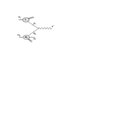
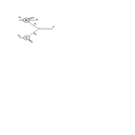
Figure 2: Pictorial representation of the parton model formula in eq. (19). The hadron $H$ is non-perturbatively produced by a fracture functions.

The integration limits of convolution integrals in both lines of eq. (19) are given by momentum conservation:

$$1-z\geq x_{1}x_{2}\geq\tau\;\;\makebox{and}\;\;x_{1}+z\leq 1\;\;\makebox{in}\;\;\mathcal{R}_{T_{1}}\,,$$ (20)

$$1-z\geq x_{1}x_{2}\geq\tau\;\;\makebox{and}\;\;x_{2}+z\leq 1\;\;\makebox{in}\;\;\mathcal{R}_{T_{2}}\,.$$ (21)

Phase space integrations are asymmetric since each fracture function selects its own fragmentation region. To uniform the notation, we exchange the superscript $H/H_{1}$ ($H/H_{2}$) for $[1]$ ($[2]$) which proves to be useful for the bookkeeping of the various contributions. Fracture functions in eq. (19) are normalized according to the constraint

$$\sum_{H}\int dz\frac{d\sigma^{H}(\tau)}{dQ^{2}dz}=\frac{d\sigma(\tau)}{dQ^{2}}\,.$$ (22)

The above constraint must me fullfilled irrespective to the order of the perturbative calculations. It is interesting to note that for the inclusive Drell-Yan cross-sections appearing on the right hand side of eq. (22), the factorization theorem guarantees that the corresponding cross-sections can be described by universal parton distributions functions. On the left hand side of eq. (22), we have instead no guarantee that fracture functions eventually extracted from Deep Inelastic Scattering can be succesfully used in hadronic collisions. Eq. (19) is therefore both a factorization and a cross-section conjecture for the process under examination. In the remainder of this section we consider the evaluation of $\mathcal{O}(\alpha_{s})$ corrections to the parton model formula, eq. (19). We address it as target contributions to distinguish them from the one evaluated in Sec. III. As already stated, when the final state hadron is observed in $\mathcal{R}_{T_{1}}$ or $\mathcal{R}_{T_{2}}$, we assume that it has been non-perturbatively produced from a fracture functions. Final state partons occurring in $\mathcal{O}(\alpha_{s})$ corrections to eq. (19) must be therefore integrated over phase space and virtual corrections added. A diagram contributing to eq. (23) is depicted in Fig. (3). The calculation closely follows the one already presented in Sec. II for the inclusive Drell-Yan process upon the exchange of a parton distributions with a fracture functions and taking into account momentum conservation in integrations limits. We therefore just quote the final result, valid up to $\mathcal{O}(\alpha_{s})$:

$$\frac{d\sigma^{T}(\tau)}{dQ^{2}dz}=\sigma_{0}\int_{\tau}^{1-z}\frac{dx_{1}}{x_{1}}\int_{\frac{\tau}{x_{1}}}^{1}\frac{dx_{2}}{x_{2}}\sum_{q}e_{q}^{2}\Bigg{\{}$$ (23)

$$\hskip 28.45274pt\Big{[}M_{q}^{[1]}(x_{1},z)f_{\bar{q}}^{[2]}(x_{2})+(q\leftrightarrow\bar{q})\Big{]}\Big{[}\delta(1-w)-\frac{2}{\epsilon}\frac{\alpha_{s}}{2\pi}P_{qq}(w)\,c_{0}+\frac{\alpha_{s}}{2\pi}\widetilde{C}_{q\bar{q}}(w)\Big{]}+$$

$$\hskip 28.45274pt\Big{[}\big{(}M_{g}^{[1]}(x_{1},z)f_{\bar{q}}^{[2]}(x_{2})+M_{q}^{[1]}(x_{1},z)f_{g}^{[2]}(x_{2})\big{)}+(q\leftrightarrow\bar{q})\Big{]}\cdot$$

$$\hskip 227.62204pt\cdot\Big{[}-\frac{1}{\epsilon}\frac{\alpha_{s}}{2\pi}P_{qg}(w)\,c_{0}+\frac{\alpha_{s}}{2\pi}\widetilde{C}_{qg}(w)\Big{]}\Bigg{\}}+$$

$$\hskip 19.91684pt+\sigma_{0}\int_{\frac{\tau}{1-z}}^{1}\frac{dx_{1}}{x_{1}}\int_{\frac{\tau}{x_{1}}}^{1-z}\frac{dx_{2}}{x_{2}}\sum_{q}e_{q}^{2}\Bigg{\{}$$

$$\hskip 28.45274pt\Big{[}M_{q}^{[2]}(x_{2},z)f_{\bar{q}}^{[1]}(x_{1})+(q\leftrightarrow\bar{q})\Big{]}\Big{[}\delta(1-w)-\frac{2}{\epsilon}\frac{\alpha_{s}}{2\pi}P_{qq}(w)\,c_{0}+\frac{\alpha_{s}}{2\pi}\widetilde{C}_{q\bar{q}}(w)\Big{]}+$$

$$\hskip 28.45274pt\Big{[}\big{(}M_{g}^{[2]}(x_{2},z)f_{\bar{q}}^{[1]}(x_{1})+M_{q}^{[2]}(x_{2},z)f_{g}^{[1]}(x_{1})\big{)}+(q\leftrightarrow\bar{q})\Big{]}\cdot$$

$$\hskip 227.62204pt\cdot\Big{[}-\frac{1}{\epsilon}\frac{\alpha_{s}}{2\pi}P_{qg}(w)\,c_{0}+\frac{\alpha_{s}}{2\pi}\widetilde{C}_{qg}(w)\Big{]}\Bigg{\}}\,.$$

Comparing eq. (4) with eq. (23) reveals that in target fragmentation region the structure of collinear singularities is the same as in the inclusive Drell-Yan case, as expected. The main change is just a restriction on phase space integrals since the production of the Drell-Yan pair of a given invariant mass $Q^{2}$ must be, by energy-momentum conservation, compatible with the observation of a hadron in the final state with fractional momentum $z$.

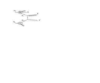
Figure 3: Example of $\mathcal{O}(\alpha_{s})$ real corrections contributing to eq. (23). The hadron $H$ is non perturbatively produced by a fracture function.

V Finite cross-sections at NLO

In this section we will describe the collinear factorization procedure which must be applied in order to get infrared finite results for the cross-section under examination. We have already noted, by comparing eq. (4) and eq. (23), that the structure of collinear singularities in the target fragmentation region is identical to the one found in the inclusive Drell-Yan case. We may expect that renormalized fracture functions are defined in a way similar to that of renormalized parton densities in eq. (6). As it was firstly obtained in the original analysis of Ref. Trentadue_Veneziano and confirmed in the one loop calculation of Ref. Graudenz , the renormalized fracture functions obey a somewhat more involved subtraction with respect to parton distributions. In the $\overline{\textrm{MS}}$ scheme the redefinition of bare fracture functions reads:

$$M_{i}^{H/H_{1}}(x,z)=\int_{x/(1-z)}^{1}\frac{du}{u}\Big{[}\delta_{ij}\delta(1-u)+\frac{1}{\epsilon}\frac{\alpha_{s}}{2\pi}\frac{\Gamma(1-\epsilon)}{\Gamma(1-2\epsilon)}\Big{(}\frac{4\pi\mu_{R}^{2}}{\mu_{F}^{2}}\Big{)}^{\epsilon}P_{ij}(u)\Big{]}M_{j}^{H/H_{1}}\Big{(}\frac{x}{u},z,\mu_{F}^{2}\Big{)}\,+\\ +\int_{x}^{x/(x+z)}\frac{du}{u}\frac{1}{1-u}\frac{u}{x}\frac{1}{\epsilon}\frac{\alpha_{s}}{2\pi}\frac{\Gamma(1-\epsilon)}{\Gamma(1-2\epsilon)}\Big{(}\frac{4\pi\mu_{R}^{2}}{\mu_{F}^{2}}\Big{)}^{\epsilon}\widehat{P}_{ij}(u)\,f_{j/H_{1}}\Big{(}\frac{x}{u}\Big{)}\,D_{l}^{H}\Big{(}\frac{zu}{x(1-u)}\Big{)}\,,$$ (24)

where in our notation $\widehat{P}_{ij}(u)=\widehat{P}_{(l)i\leftarrow j}(u)$. The first term on r.h.s of eq. (24) has the same subtraction structure as for parton distribution, eq. (6). The singularity is due to collinear radiation accompaining the active parton, while the hadron in the final state is non perturbatively produced by the fracture functions itself. In the second term of eq. (24) the singularity is due configurations in which the parent parton of the observed hadron is collinear to the incoming parton. The factorization procedure is accounted for by substituting in eq. (23) the bare fracture and distributions functions by their renormalized version in eq. (6) and eq. (24). Renormalized parton distributions and fracture functions homogeneous terms do cancel all singularities present in eq. (23). The additional singularities in eq. (15) are cancelled by the combination of parton distributions and fracture functions inhomogeneous renormalization terms. The final result, up to order $\mathcal{O}(\alpha_{s})$, is obtained adding the the various contributions:

$$\frac{d\sigma^{H}(\tau)}{dQ^{2}dz}=\frac{d\sigma^{H,T}(\tau)}{dQ^{2}dz}\;+\;\frac{d\sigma^{H,C}(\tau)}{dQ^{2}dz}=\sigma_{0}\sum_{q}e_{q}^{2}\Bigg{\{}$$ (25)

$$\int_{\tau}^{1-z}\frac{dx_{1}}{x_{1}}\int_{\frac{\tau}{x_{1}}}^{1}\frac{dx_{2}}{x_{2}}\bigg{\{}\Big{[}M_{q}^{[1]}(x_{1},z,\mu_{F}^{2})f_{\bar{q}}^{[2]}(x_{2},\mu_{F}^{2})+(q\leftrightarrow\bar{q})\Big{]}\Big{[}\delta(1-w)+\frac{\alpha_{s}}{2\pi}C_{q\bar{q}}\Big{(}w,\frac{\mu_{F}^{2}}{Q^{2}}\Big{)}\Big{]}+$$

$$\hskip 28.45274pt\Big{[}\big{(}M_{g}^{[1]}(x_{1},z,\mu_{F}^{2})f_{\bar{q}}^{[2]}(x_{2},\mu_{F}^{2})+M_{q}^{[1]}(x_{1},z,\mu_{F}^{2})f_{g}^{[2]}(x_{2},\mu_{F}^{2})\big{)}+(q\leftrightarrow\bar{q})\Big{]}\frac{\alpha_{s}}{2\pi}C_{qg}\Big{(}w,\frac{\mu_{F}^{2}}{Q^{2}}\Big{)}\bigg{\}}+$$

$$\int_{\frac{\tau}{1-z}}^{1}\frac{dx_{1}}{x_{1}}\int_{\frac{\tau}{x_{1}}}^{1-z}\frac{dx_{2}}{x_{2}}\bigg{\{}\Big{[}M_{q}^{[2]}(x_{2},z,\mu_{F}^{2})f_{\bar{q}}^{[1]}(x_{1},\mu_{F}^{2})+(q\leftrightarrow\bar{q})\Big{]}\Big{[}\delta(1-w)+\frac{\alpha_{s}}{2\pi}C_{q\bar{q}}\Big{(}w,\frac{\mu_{F}^{2}}{Q^{2}}\Big{)}\Big{]}+$$

$$\hskip 28.45274pt\Big{[}\big{(}M_{g}^{[2]}(x_{2},z,\mu_{F}^{2})f_{\bar{q}}^{[1]}(x_{1},\mu_{F}^{2})+M_{q}^{[2]}(x_{2},z,\mu_{F}^{2})f_{g}^{[1]}(x_{1},\mu_{F}^{2})\big{)}+(q\leftrightarrow\bar{q})\Big{]}\frac{\alpha_{s}}{2\pi}C_{qg}\Big{(}w,\frac{\mu_{F}^{2}}{Q^{2}}\Big{)}\bigg{\}}+$$

$$\int_{0}^{1}dy\int_{r_{1}}^{1}\frac{dx_{1}}{x_{1}}\int_{r_{2}}^{1}\frac{dx_{2}}{x_{2}}\bigg{\{}\Big{[}f_{q}^{[1]}(x_{1},\mu_{F}^{2})\,f_{\bar{q}}^{[2]}(x_{2},\mu_{F}^{2})+(q\leftrightarrow\bar{q})\Big{]}\,D_{g}^{H}\big{(}z/\rho,\mu_{F}^{2}\big{)}\frac{\alpha_{s}}{2\pi}K_{q\bar{q}}\Big{(}y,\frac{\mu_{F}^{2}}{Q^{2}}\Big{)}+$$

$$\hskip 99.58464ptf_{g}^{[1]}(x_{1},\mu_{F}^{2})\Big{[}f_{\bar{q}}^{[2]}(x_{2},\mu_{F}^{2})D_{\bar{q}}^{H}\big{(}z/\rho,\mu_{F}^{2}\big{)}+(q\leftrightarrow\bar{q})\Big{]}\,\frac{\alpha_{s}}{2\pi}K_{qg}\Big{(}y,\frac{\mu_{F}^{2}}{Q^{2}}\Big{)}+$$

$$\hskip 99.58464ptf_{g}^{[2]}(x_{2},\mu_{F}^{2})\Big{[}f_{\bar{q}}^{[1]}(x_{1},\mu_{F}^{2})D_{\bar{q}}^{H}\big{(}z/\rho,\mu_{F}^{2}\big{)}+(q\leftrightarrow\bar{q})\Big{]}\,\frac{\alpha_{s}}{2\pi}K_{qg}\Big{(}1-y,\frac{\mu_{F}^{2}}{Q^{2}}\Big{)}\bigg{\}}\Bigg{\}}\,.$$

We have used the shorthand $K_{ij}(y,\mu_{F}^{2}/Q^{2})$ for $K_{ij}(y,x_{1},x_{2},w,\mu_{F}^{2}/Q^{2})$. The explicit form of the finite coefficient functions $K_{q\bar{q}}$ and $K_{qg}$ is reported in appendix A. In the last three lines of eq. (25) we let depend parton distributions and fragmentation functions on the factorization scale since this replacement induces subleading corrections to the current accuracy.

VI Summary and Conclusions

In this paper we have calculated the $\mathcal{O}(\alpha_{s})$ corrections to the associated production of one particle and a Drell-Yan pair. Additional collinear singularities found in the perturbative calculations do correspond to configurations in which the parent parton of the observed hadron is collinear to the incoming parton. These singularities can, to $\mathcal{O}(\alpha_{s})$, be consistently absorbed into renormalized fracture functions and resummed to all orders by using the evolution equation given in Refs. Trentadue_Veneziano ; Graudenz . With this technique, the presented cross-sections does not require any cut in the transverse momentum of the observed particle, while a perturbative treatment is guarantee by the presence of high invariant mass dilepton pair. Quite imprtantly, the factorization of collinear singularities in the present context makes use of the collinear subtraction structure already defined in the context of Deep Inelastic Scattering. Despite the fact the the full results make use of fracture functions and threfore a phenomenological modelling of the latter would be eventually required, the advatages reside in that fracture functions embodies the correct scale dependence through their own evolution equations.

Appendix A Finite coefficients

In this Appendix we present the results for the finite coefficient which appear in the previous sections. The plus distribution are defined in the usual way:

$$\int_{0}^{1}dw\frac{h(w)}{(1-w)_{+[0,\underline{1}]}}\equiv\int_{0}^{1}dw\frac{h(w)-h(1)}{1-w}.$$ (26)

The subtraction point is underlined. The coefficient functions in the target fragmentation region do coincide with the one found in the inclusive case and read:

$$C_{q\bar{q}}\Big{(}w,\frac{\mu_{F}^{2}}{Q^{2}}\Big{)}=-2P_{qq}(w)\ln\frac{\mu_{F}^{2}}{Q^{2}}+\widetilde{C}_{q\bar{q}}(w)\,,$$

$$C_{qg}\Big{(}w,\frac{\mu_{F}^{2}}{Q^{2}}\Big{)}=-P_{qg}(w)\ln\frac{\mu_{F}^{2}}{Q^{2}}+\widetilde{C}_{qg}(w)\,,$$ (27)

where the scale independent coefficients $\widetilde{C}_{ij}$ are given by:

$$\widetilde{C}_{q\bar{q}}(w)=C_{F}\Bigg{[}4(1+w^{2})\Bigg{(}\frac{\ln(1-w)}{1-w}\Bigg{)}_{+[0,1]}-2\frac{1+w^{2}}{1-w}\ln w+\Big{(}\frac{2}{3}\pi^{2}-8\Big{)}\delta(1-w)\Bigg{]}\,,$$

$$\widetilde{C}_{qg}(w)=T_{R}\Bigg{[}\big{(}w^{2}+(1-w)^{2}\big{)}\ln\frac{(1-w)^{2}}{w}+\frac{1}{2}+3w-\frac{7}{2}w^{2}\,\Bigg{]}\,.$$ (28)

The polynomial term in $C_{qg}$ is slightly different from the one reported in Ref. DYNLO because an additional term $(1-\epsilon)^{-1}$ is provided for matrix elements with a gluon in the initial state. This accounts for the correct gluon polarization in $n$-dimensions and it affects only the polynomial terms in the coefficient function. For the central term the subtraction is performed on the angular variable $y$. The plus distributions in eq. (16) are defined by:

$$\int_{0}^{1}dy\frac{h(y)}{(1-y)_{+[0,\underline{1}]}}\equiv\int_{0}^{1}dy\frac{h(y)-h(1)}{1-y}\,,$$ (29)

$$\int_{0}^{1}dy\frac{h(y)}{(y)_{+[\underline{0},1]}}\equiv\int_{0}^{1}dy\frac{h(y)-h(0)}{y}\,,$$ (30)

where $h(y)$ is a smooth test function. The coefficients $K_{ij}$ read:

$$K_{q\bar{q}}\Big{(}y,x_{1},x_{2},\tau,\frac{\mu_{F}^{2}}{Q^{2}}\Big{)} = \widetilde{K}_{q\bar{q}}(y,x_{1},x_{2},\tau)+$$

$$-\delta(y)\widehat{P}_{qq}(w)\frac{x_{2}}{x_{1}x_{2}-\tau}\ln\frac{\mu_{F}^{2}}{Q^{2}}-\delta(1-y)\widehat{P}_{qq}(w)\frac{x_{1}}{x_{1}x_{2}-\tau}\ln\frac{\mu_{F}^{2}}{Q^{2}}\,;$$

$$K_{qg}\Big{(}y,x_{1},x_{2},\tau,\frac{\mu_{F}^{2}}{Q^{2}}\Big{)} = \widetilde{K}_{qg}(y,x_{1},x_{2},\tau)-\delta(y)\frac{x_{2}}{x_{1}x_{2}-\tau}\widehat{P}_{qg}(w)\ln\frac{\mu_{F}^{2}}{Q^{2}}\,.$$ (31)

By defining $b(x_{1},x_{2},y)=x_{1}y+x_{2}(1-y)$ and $a=x_{1}x_{2}-\tau$, the scale-independent $\widetilde{K}_{ij}$ coefficients read:

$$\widetilde{K}_{q\bar{q}}(y,x_{1},x_{2},\tau) = C_{F}\Bigg{\{}\frac{1}{b}\Bigg{(}\frac{x_{2}}{x_{1}}(1-y)+\frac{2\tau b^{2}}{a^{2}}\Bigg{)}\,\frac{1}{y_{+[\underline{0},1]}}+\frac{1}{b}\Bigg{(}\frac{x_{1}}{x_{2}}y+\frac{2\tau b^{2}}{a^{2}}\Bigg{)}\frac{1}{(1-y)_{+[0,\underline{1}]}}+$$

$$+\,\delta(y)\Bigg{[}\frac{1}{x_{1}}-\frac{1+w^{2}}{1-w}\frac{x_{2}}{a}\ln\frac{x_{2}^{2}\tau}{a^{2}}\Bigg{]}+\delta(1-y)\Bigg{[}\frac{1}{x_{2}}-\frac{1+w^{2}}{1-w}\frac{x_{1}}{a}\ln\frac{x_{1}^{2}\tau}{a^{2}}\Bigg{]}\Bigg{\}}\,;$$

$$\widetilde{K}_{qg}\Big{(}y,x_{1},x_{2},\tau) = T_{R}\Bigg{\{}\Bigg{(}\frac{x_{2}}{a}-\frac{2(1-y)\tau}{bx_{1}^{2}}\Bigg{)}\frac{1}{y_{+[\underline{0},1]}}+\frac{ay}{x_{2}b^{2}}+$$ (32)

$$+\delta(y)\frac{x_{2}}{a}\Bigg{[}1-\Big{[}w^{2}+(1-w)^{2}\Big{]}\Bigg{(}\ln\frac{\tau x_{2}^{2}}{a^{2}}+1\Bigg{)}\Bigg{]}\Bigg{\}}\,.$$

The coefficient function $K_{gq}$ can be obtained by exchanging $x_{1}\leftrightarrow x_{2}$ and $y\leftrightarrow 1-y$ in the expressions for $K_{qg}$. In $K_{q\bar{q}}$ one can note the appearance of poles in $(1-w)^{-1}$, where $w=\tau/(x_{1}x_{2})$. In this limit only soft parton emissions are allowed. This limit however is outside the integration region specified in the central contribution to the final result, eq. (25), due to the requirement $z>0$ embodied in the specific form of the integration boundaries $r_{1}$ and $r_{2}$ in eqs. (III).

References

• (1) R. Sassot et al., arXiv:1008.0540  .
• (2) D. Graudenz, Nucl. Phys.  B432 (1994) 351 .
• (3) L. Trentadue, G. Veneziano, Phys. Lett.  B323 (1994) 201 .
• (4) W. T. Giele et al., Nucl. Phys.  B403 (1993) 633 .
• (5) C. F. Berger et al., Phys. Rev. Lett.  102 (2009) 222001 .
• (6) M. Cacciari et al., JHEP (2010) 1004:065 .
• (7) F. A. Ceccopieri, L. Trentadue, Phys. Lett.  B655 (2007) 15 .
• (8) G. Camici, M. Grazzini, L. Trentadue, Phys. Lett.  B439 (1998) 382  .
• (9) F. A. Ceccopieri, L. Trentadue,  Phys. Lett.  B668 (2008) 319 .
• (10) S. D. Drell, T. Yan  Phys. Rev. Lett.  25 (1970) 316 . Erratum-ibid. 25 (1970) 902 .
• (11) G. Altarelli, R. K. Ellis, G. Martinelli, Nucl. Phys.  B157 (1979) 461 .
• (12) L.N. Lipatov, Sov. J. Nucl. Phys.  20 95 (1975) 95 ;
V.N. Gribov and L.N. Lipatov, Sov. J. Nucl. Phys.  15 (1972) 438 ;
G. Altarelli and G. Parisi, Nucl. Phys.  B126 (1977) 298 ;
Yu.L. Dokshitzer Sov. Phys. JETP  46 (1977) 641 .
• (13) F. Aversa, et al. Nucl.Phys. B327 (1989) 105 .
• (14) K. Konishi, A. Ukawa, G. Veneziano, Nucl. Phys.  B157 (1979) 45 .
• (15) J. C. Collins, Phys. Rev.  D57 (1998) 3051 .
• (16) M. Grazzini, L. Trentadue, G. Veneziano, Nucl. Phys.  B519 (1998) 394 .