Feasibility and performances of compressed-sensing and sparse map-making with Herschel/PACS data

The Herschel Space Observatory of ESA was launched in May 2009 and is in operation since. From its distant orbit around L2 it needs to transmit a huge quantity of information through a very limited bandwidth. This is especially true for the PACS imaging camera which needs to compress its data far more than what can be achieved with lossless compression. This is currently solved by including lossy averaging and rounding steps on board. Recently, a new theory called compressed-sensing emerged from the statistics community. This theory makes use of the sparsity of natural (or astrophysical) images to optimize the acquisition scheme of the data needed to estimate those images. Thus, it can lead to high compression factors.

A previous article by Bobin et al. (2008) showed how the new theory could be applied to simulated Herschel/PACS data to solve the compression requirement of the instrument. In this article, we show that compressed-sensing theory can indeed be successfully applied to actual Herschel/PACS data and give significant improvements over the standard pipeline. In order to fully use the redundancy present in the data, we perform full sky map estimation and decompression at the same time, which cannot be done in most other compression methods. We also demonstrate that the various artifacts affecting the data (pink noise, glitches, whose behavior is a priori not well compatible with compressed-sensing) can be handled as well in this new framework. Finally, we make a comparison between the methods from the compressed-sensing scheme and data acquired with the standard compression scheme. We discuss improvements that can be made on ground for the creation of sky maps from the data.

1 Introduction

The Herschel Space Observatory (Pilbratt et al., 2010) is a three and a half year mission carrying instruments to observe in the far-infrared. It is dedicated to the investigation of galaxy formation and evolution mechanisms, star formation and interaction with the interstellar medium, molecular chemistry in the universe and finally chemical analysis of the atmospheres of bodies of the Solar System. With its 3.5 m telescope, Herschel is the largest space observatory to date. Its three instruments are: the Photodetector Array Camera and Spectrometer (PACS) (Poglitsch et al., 2010), the Spectral and Photometric Imaging Receiver (SPIRE), (Griffin et al., 2010), and the Heterodyne Instrument for the Far Infrared (HIFI) (de Graauw et al., 2010).

Due to power and dissipation constraints, routine operations on Herschel see only one instrument powered per observing day (OD). A special mode exists, called the SPIRE$+$PACS parallel mode (see below), where both SPIRE and PACS can be operated. The duty-cycle of Herschel rests on the concept of the OD, which typically consists in a period of autonomous observations of 20-22 h, and a daily telecommunication period (DTCP) of 2-4 h during which the data recorded on board is downlinked and the program of the next ODs is uplinked (Herschel always stores on-board the program of its next two ODs, in case of problems during the DTCP).

Limits to the amount of data that can be generated by the instruments are imposed by (1) the speed of the internal communication links between the instruments and the service module, and (2) the speed and duration of the communication link between the satellite and its ground stations. These limits translates typically in an acceptable average data rate for the instrument during the OD of 130 kbit/s, while the PACS photometer, featuring the largest number of pixels ($\sim$2500) and a high sampling frequency (40 Hz) provides a native data rate of 1600 kbit/s, to which 40 kbit/s have to be added for housekeeping information. The situation is even more complex for the PACS spectrometer at 4000 kbit/s (but the integration ramps can be compressed on-board in a natural fashion), while SPIRE and HIFI have much smaller data rates around or below 100 kbit/s, requiring no compression on board.

We focus on the PACS imaging camera, which is made of two arrays of bolometers operating in the 55 to 210 $\mu$m range. Due to the above restrictions PACS data need to be compressed by a factor of 16 to 32. For this purpose, on-board data reduction and compression is carried out by dedicated sub-units (Ottensamer & Kerschbaum, 2008).

In this paper, we investigate alternative compression modes to attain such a high compression factor without sacrificing noise or resolution. The study in this paper is based on the theory of compressed-sensing and represents a real-world implementation of ideas presented in Bobin et al. (2008). Simply put, compressed-sensing is a promising theory which leverages the sparsity properties of data to allow measurements beyond the Shannon-Nyquist limit (Donoho, 2006; Candès, 2008). In the context of PACS, it offers potential to optimize on-board compression. It has the very strong advantage that it is not computationally expensive on the acquisition side, a very important point for a space mission. An additional constraint for PACS is that CS had to be implemented after the conception of the instrument, while the instrument hardware cannot be changed as well as most of the on-board software.

We first present the PACS instrument, describe the properties of its data, and explain how we model the instrument. Then, we explain how we perform map-making using PACS data which is a central stage in data analysis. Finally, we introduce our compressed-sensing implementation and we show how the map-making process can be modified in the compressed-sensing framework to estimate state-of-the-art or better sky maps.

2 PACS data

2.1 The PACS imaging camera

The PACS imaging camera is made of two arrays of bolometers. One array is made of two $16\times 16$ matrices forming a $32\times 16$ array. It is associated with the “red” filter ranging from 130 to 210 $\mu$m. The other array is made of eight $16\times 16$ matrices and thus has a shape of $64\times 32$ pixels. It is associated with the filters “green” and “blue” ranging respectively from 85 to 130 $\mu$m and from 60 to 85 $\mu$m. Figure (3) shows a single frame of the PACS blue array.

The PACS camera can be used in two modes: the chop-nod mode and the scan mode. The chop-nod mode consists in using an internal chopper to alternate between two sky positions (ON and OFF) and the satellite to exchange the ON and OFF beam positions. It was originally dedicated to the observation of point sources, with the chop-nod modulation used to get rid of the low-frequency noise originating in the detector. However it turned out that even for point sources, scan-mode observations are more efficient in terms of achieved sensitivity for a given observing time. Therefore this mode is not considered here. The scan mode scans the sky in order to observe larger areas than the detector field-of-view. When PACS is the only instrument powered, the prime mode, there are three possible scan speeds: 10, 20 and 60 arcsec/s. The PACS camera can also work in scan mode in conjunction with SPIRE, the parallel mode, in which case observations are driven by SPIRE requirements and the scan speed is either 30 or 60 arcsec/s. Most of the PACS data are therefore obtained in scan mode, either in prime or parallel mode, and in any case, the bolometer arrays are read at 40 Hz.

The data are compressed using a lossless entropic compression scheme which yields up to a factor of 4, requiring another factor of 4 (8 in parallel mode) to be achieved with lossy steps. For this purpose, 4 (or 8) consecutive frames are averaged before lossless compression. Additionally, a bit-rounding step is performed. It consists in rounding the averaging that is performed on board so that the number of bits required to encode the data is reduced by 1 or 2 bits. This rounding is randomly up and down so as to not bias the results. In prime mode, one bit is removed while in parallel mode two bits are removed. We will not consider the bit-rounding operation in this article. In parallel mode an averaging of 8 frames is required because the satellite bandwidth is shared with SPIRE. In fast parallel mode, this averaging results in a blurring of the frames and thus a loss of resolution in the sky maps which is highly undesirable. Indeed, in this mode the scan speed can be 60 arcsec/s, or 18.75 pixels/s. Frames are taken at 40 Hz, thus the displacement between two frames is approximately 0.5 pixel. In parallel mode 8 frames are averaged with a total motion of around 4 pixels. This is very significant compared to the point-spread function (PSF) in the blue filter which has a full-width at half maximum (FWHM) of 1.6 pixels.

This blurring is a very strong incentive to investigate other compression schemes. Presently, it can be avoided only by configuring the so-called transparent compression mode, where only one-eighth of the frame area is transmitted, but at full temporal resolution. With this mode we can experiment with all the stages of the acquisition while incorporating all features and artifacts of the actual instrument.

Indeed, care must be taken when using a new acquisition or compression mode that it will not decrease our ability to separate the signal of interest from instrumental artifacts. PACS imaging data have some properties that have to be taken into consideration. The most salient one is a large signal offset that varies for each pixel. The dispersion of the offset among the detectors occupies half of the range of values allowed by the 16 bits digitisation, whereas the typical signal range is around 15 bits with a noise entropy of 4-6 bits. This noise measurement is not a theoretical value, but the entropy of decorrelated measured data. It has been determined in two ways : computing the Shannon entropy of the difference signal minus 0.5 bit (Differentiation increases the sigma by a factor $\sqrt{(}2)$ or half a bit in entropy, which needs to be subtracted to get the original value) and computing the Shannon entropy of the high-frequency coefficients of a wavelet (for example Haar) transform. Both methods give almost the same value. This is essentially the readout noise, so it does not take into account the pink component of the noise which can be seen at longer time scales. Hence, the quantization noise is not negligible with respect to the signal and adds to the other sources of noise. As can be seen in Figure 3a, the signal of interest is not visible when the offset is not removed and we cannot subtract it on board. If the offset is removed (Figure 3b), it is still hard to detect physical structure because of the noise. Some glitches can be identified however that could not be seen in Figure 3a. It corresponds to the high-valued isolated pixels.

Furthermore, there is a drift of this offset (Figure 1) which can be seen as pink noise ($1/f$ noise). More precisely, it is a $1/f^{1/2}$ noise as its power spectrum decreases with the inverse of the square root of the frequency. One of the main issues in PACS data processing is the separation of the signal from this drift. Its amplitude is of the order of magnitude of the signal of interest. In addition, this pink noise is affecting all the temporal frequencies in the PACS bandwidth. In other words, the transition between pink noise and white noise is happening at higher frequencies than the sampling frequency of PACS.

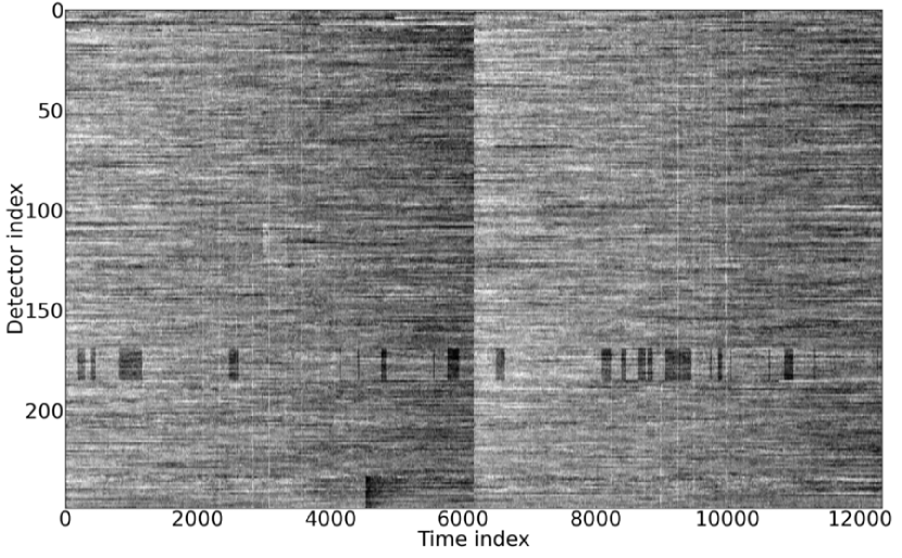
Figure 1: Data set of the PACS imaging camera in the blue band in the transparent mode. This set consists of two cross-scans. The offset has been removed. All pixels have been reordered in a vector shape and displayed as a function of time (so that each pixel is shown as a horizontal line). Horizontal structures are the drift of the offset. The discontinuity in the offsets at the center of the figure comes from the temporal gap between the two cross-scans. An unstable line (pixels 176 to 192) results in frequent intensity discontinuities along both scans. At time index 45000 the additional drift is due to a cosmic ray hit in the multiplexing electronics affecting a whole line. Finally, the faint vertical structures are due to the bright galaxy nucleus passing in front of the detectors.

Once the offset is removed, other features become visible, as can be seen in Figure 1. For instance, the bad behavior of a whole line of pixels results in frequent discontinuities of the intensity as a function of time (pixels 176 to 192 in the figure). A cosmic ray hit in the electronics of the last line around the time index 45000 results in an additional drift of these pixels. Other cosmic rays can hit individual detectors and be the cause of wrong intensity values (outliers). However, those cosmic ray hits are affecting less than 1 percent of the data due to the spatial structure of the detector elements (they are hollow). Outliers due to cosmic rays are usually filtered out by comparing the set of data values corresponding to one map pixel and masking values beyond a threshold (see section 5.2 for details).

The faint vertical structures in Figure 1 are in fact the nucleus of the galaxy which passes in front of the detectors multiple times. Only the nucleus is bright enough to be visible in the offset removed data. Projection of the data onto the sphere of the sky as well as filtering of the $1/f^{1/2}$ noise are required in order to see the fainter parts. After the projection, the contributions of each pixel at each time index add up in order to greatly increase the visibility of the fainter objects.

2.2 Instrument model

Our optimal reconstruction scheme requires an understanding of the acquisition process, done here with an instrument model.

For the rest of this article, the data sets and the sky maps are vectorized (i.e. re-indexed). Vectors are represented as bold lower-case letters. Linear operators are represented as matrices and written in bold upper-case letters.

The PACS data are a set of samples of the bolometers taken at different times and thus at different positions in the sky (in scan mode). Each sample is proportional to the sky surface brightness and to the area of the detector projected on the sky sphere (see Figure 2). Thus, PACS data and the flux of the sky are linearly related and we can write equation (1) where ${\mathb{y}}$ stands for the data, ${\mathb{x}}$ denotes the sky pixels values and ${\mathb{P}}$ is the projector. The noise is considered additive and is noted ${\mathb{n}}$.

$${\mathb{y}}={\mathb{P}}{\mathb{x}}+{\mathb{n}}$$ (1)

We take into account the distortion of the field of view (FOV) by the optics of the instrument in the projector. The gains of the bolometers can be taken into account too. In our formalism, we would simply multiply ${\mathb{P}}$ by a diagonal matrix with the gain map on the diagonal (assuming that the gain does not vary with time, the gain map would simply be the flat-field repeated n_f times, where n_f is the number of frames). The compression will be taken into account separately.

In this paper, we used an implementation of the PACS instrument model provided by Chanial (2010) in preparation.

Figure 2: Sketch of the intersection of the sky map pixel $i$ and detector $j$. The matrix element $(i,j)$ of the projection matrix ${\mathb{P}}$ is equal to the intersecting area of the pixel $i$ with the detector $j$. The sky map pixels are square but the detectors are quadrilaterals because of the distortion of the optics. The distortion is exaggerated in this sketch.

3 Map-making

The map-making stage is the inverse problem associated with equation (1), that is the estimation of ${\mathb{x}}$ knowing ${\mathb{y}}$. It can be computed using classical estimation methods. We now review some of the methods that have been implemented for the map-making stage.

3.1 PACS pipeline

The Herschel Interactive Processing Environment (HIPE) offers back-projection of the data onto the sky map for the map-making pipeline step. In order to guarantee the conservation of the flux, the map must be divided by the coverage map (that is the number of times a pixel of the sky map has been seen by the detectors). The sky map estimation using the pipeline is thus described by equation (2).

$$\hat{{\mathb{x}}}_{pipeline}=\frac{{\mathb{P}}^{T}{\mathb{y}}}{{\mathb{P}}^{T}\mathbf{1}}$$ (2)

Estimated sky maps are noted with a $\hat{\cdot}$. $\cdot^{T}$ is the transpose of a matrix, $\mathbf{1}$ is a vector of ones. The division of two vectors here is the term by term division of their coefficients.

This method is very fast and straightforward to implement. But it does not provide a very accurate estimate of the sky. To illustrate this, one could compare this estimate to the least-squares estimate of the sky map. The least-squares estimate minimizes the criterion $\|{\mathb{y}}-{\mathb{P}}{\mathb{x}}\|^{2}$ and can be written in closed form as in equation (3). The least-squares solution can be seen as the maximum likelihood solution under the assumption of independent and identically distributed Gaussian noise.

$$\hat{{\mathb{x}}}_{lsq}=\left({\mathb{P}}^{T}{\mathb{P}}\right)^{-1}{\mathb{P}}^{T}{\mathb{y}}$$ (3)

The pipeline solution can now be interpreted as a very crude approximation of the least-squares solution by replacing the inversion of ${\mathb{P}}^{T}{\mathb{P}}$ by the inversion of the coverage map. This approximation ignores the correlations introduced by the projection matrix. In a more physical interpretation, one can say that the pipeline solution does not take into account the possibility to make use of super-resolution from the PACS data. Reducing the pixel size in the pipeline sky map will not help on this matter. The projection matrix inversion is required. In fact, the PSF is not always sampled at the Nyquist-Shannon frequency and it is thus possible to obtain a better resolution in the sky map than in the raw data. As can be seen in Table 1 this is mainly beneficial for the blue filter (70 $\mu$m) in which aliasing occurs the most.

filter	70 $\mathbf{\mu}$m	100 $\mathbf{\mu}$m	160 $\mathbf{\mu}$m
wavelength range ($\mu$m)	60–85	85–130	130–210
resolution ($\lambda/\Delta\lambda$)	$\sim$ 3		$\sim$ 2
pixel size (arcsec)	3.2		6.4
FOV (arcmin)	3.5 $\times$ 1.75
FWHM	5.2	7.7	12

Table 1: PACS photometer overall characteristics/performances (taken from the PACS Observer’s Manual). The resolution is the spectral resolution of the bandwidth.

3.2 MADmap

There is another approach called MADmap (Cantalupo et al., 2010) which tries to better estimate the sky map. It makes use of a preconditioned conjugate gradient in order to efficiently estimate the least-squares solution. Furthermore, MADmap adds a more accurate model of the pink noise. The noise is modeled as a multivariate normal distribution with a covariance matrix ${\mathb{D}}$ diagonal in Fourier space (equation (4)). Noting ${\mathb{F}}$ the matrix of the Fourier transform along the time axis, ${\mathb{F}}^{\dagger}$ its conjugate transpose (and also its inverse), $\mathop{\mathrm{diag}}$ the operator which transforms vectors into diagonal matrices and $\tilde{\cdot}$ the Fourier transform of a vector or a matrix, we have:

$${\mathb{n}}=\mathcal{N}(\mathbf{0},{\mathb{D}})\text{, }{\mathb{D}}={\mathb{F}}^{\dagger}\tilde{{\mathb{D}}}{\mathb{F}}={\mathb{F}}^{\dagger}\mathop{\mathrm{diag}}(\tilde{{\mathb{d}}}){\mathb{F}}$$ (4)

This allows to store the full covariance matrix in an array of the size of the data, by storing the diagonal elements of the Fourier transform of ${\mathb{D}}$, which we note here $\tilde{{\mathb{d}}}$.

The map estimation in this case can be rewritten as a simple least-squares estimation following equation (3.2).

$${\mathb{y}}^{\prime} \leftarrow {\mathb{D}}^{\frac{1}{2}}{\mathb{y}}$$

$${\mathb{P}}^{\prime} \leftarrow {\mathb{D}}^{\frac{1}{2}}{\mathb{P}}$$

$$\hat{{\mathb{x}}}_{MADmap} = \left({\mathb{P}}^{T}{\mathb{D}}{\mathb{P}}\right)^{-1}{\mathb{P}}^{T}{\mathb{D}}^{\frac{1}{2}}{\mathb{y}}$$ (5)

$$= \left({\mathb{P}}^{\prime T}{\mathb{P}}^{\prime}\right)^{-1}{\mathb{P}}^{\prime T}{\mathb{y}}^{\prime}$$

${\mathb{D}}^{\frac{1}{2}}$ is such that ${\mathb{D}}^{\frac{1}{2}}{\mathb{D}}^{\frac{1}{2}}={\mathb{D}}$.

The difficulty resides in finding a proper estimation for the noise covariance matrix. One has to assume that the noise covariance matrix is time invariant at very long time scales in order to have enough data samples for its estimation. In addition, one has to assume that there is only noise in the data taken to estimate the noise covariance matrix.

For Herschel/PACS data, we have data sets close enough to pure noise data so that estimating the noise statistics is not an issue. In principle, the noise covariance matrix should be of the size of the data set since the $1/f$ noise extends to the largest scales. In practice we can perform a median filtering at very large scales and use the noise covariance matrix estimation for intermediate scales. The median filter window can be made large enough to avoid filtering any scale corresponding to the physical sources of interest. This is easier for unresolved point sources but even for extended emission the scales of interest do not exceed the size of the map.

Furthermore, the current MADmap implementation does not make use of an accurate projection matrix but assumes a one-to-one pixel association between sky map pixel and data pixel. This limits the capacity of MADmap to take advantage of the super-resolution possibilities of PACS data since the projection matrix is not accurate. Another limitation of MADmap is due to the temporal-only Fourier transform. Because of it, the covariance matrix can only model temporal correlation, neglecting detector to detector correlations, which have to be removed by some pre-processing. However, most are gone after median filtering.

4 Compressed-Sensing

4.1 Theory

It is now well known that natural images and astronomical images can be sparsely represented in wavelet bases. This finding has been successfully applied to a number of problems and to compression in particular (JPEG2000 (Skodras et al., 2001) or Dirac video compression (Borer & Davies, 2005)). But, until recently, it had not been realized that it is possible to make use of this knowledge to derive more efficient data acquisition schemes. This is precisely the idea behind the compressed-sensing (CS) theory. Compressed-sensing states that if a signal is sparse in a given basis, it can be recovered using fewer samples than would be required by the Shannon-Nyquist theorem, hence the term compressed-sensing. See Candes & Wakin (2008) for a tutorial introducing compressed-sensing theory or Candès (2006) and Donoho (2006) for seminal articles. You can also look at Starck et al. (2010) which have a lot of example applications in astrophysics.

More formally, let us assume that our signal of interest ${\mathb{x}}$ is sparse in the basis ${\mathb{B}}$ and we are taking samples ${\mathb{y}}$ through the measuring matrix ${\mathb{A}}$ (i.e. ${\mathb{y}}={\mathb{A}}{\mathb{x}}$). In this context sparse means that ${\boldsymbol{\alpha}}={\mathb{B}}{\mathb{x}}$ have few non-zero elements. ${\boldsymbol{\alpha}}$ is said to be approximately sparse if it has few “significant” elements (far from zero). The theory proposes two categories of measurement matrices that allow precise estimation of ${\mathb{x}}$ : incoherent matrices and random matrices. Random measurements are likely to give incoherent measurements. Incoherence is the fundamental requirement for ${\mathb{A}}$ in the compressed-sensing framework. Quantitatively, it means that the mutual coherence $\mu=max_{j,k}\|{\mathb{m}}_{j}^{T}{\mathb{b}}_{k}\|$ is low where ${\mathb{m}}_{j}$ and ${\mathb{b}}_{k}$ are the columns of ${\mathb{A}}$ and ${\mathb{B}}$ respectively. Under the assumptions of exact sparsity and incoherence, it can be shown that ${\mathb{x}}$ can be estimated exactly using few measurements. Precisely, if $m$ is the number of measurements, s is the number of non-zero elements and n the number of unknowns, we need $m\geq C\cdot\mu^{2}\cdot s\cdot log(n)$, where $C$ is a constant (Candès & Wakin, 2008). Under the approximate sparsity hypothesis, good performances can be demonstrated too (Stojnic et al., 2008).

In order to get the benefits of CS it is assumed that it is possible to solve the inverse problem under the assumption of sparsity (i.e. to find a sparse solution to the inverse problem). In other word, we need to find the solution of problems of the type of equation (6).

$$\hat{{\mathb{x}}}_{CS}=\displaystyle\mathop{\mathrm{arg\,min}}_{{\mathb{x}}}{\|{\mathb{B}}{\mathb{x}}\|_{0}}\text{ subject to }\|{\mathb{y}}-{\mathb{A}}{\mathb{x}}\|^{2}<\epsilon$$ (6)

where $\|\cdot\|_{0}$ is the L₀ norm which is the number of non-zero elements of the vector and $\epsilon$ is a small value linked to the variance of the signal. This estimation problem is of combinatorial complexity (all solutions need to be tested) and thus is intractable for our applications.

Since equation (6) is of combinatorial complexity, it is often replaced by equation (7) (see Bruckstein et al. (2009)), where the L₀ norm has been replaced by the L₁ norm ( $\|\|_{1}$ is the L₁ norm), or the sum of the absolute values of the coefficients.

$$\hat{{\mathb{x}}}_{CS}=\displaystyle\mathop{\mathrm{arg\,min}}_{{\mathb{x}}}{\|{\mathb{B}}{\mathb{x}}\|_{1}}\text{ subject to }\|{\mathb{y}}-{\mathb{A}}{\mathb{x}}\|^{2}<\epsilon$$ (7)

We can choose to write the estimation problem as in equation (8). It can be seen as a reformulation of equation (7) using Lagrange multipliers. Statistically, it can also be seen as the co-log-posterior (the opposite of the logarithm of the posterior distribution) of an inverse problem assuming a normal likelihood and a Laplace prior.

$$\hat{{\mathb{x}}}_{CS}=\displaystyle\mathop{\mathrm{arg\,min}}_{{\mathb{x}}}{\|{\mathb{y}}-{\mathb{A}}{\mathb{x}}\|^{2}+\lambda\|{\mathb{B}}{\mathb{x}}\|_{1}}$$ (8)

Note that this modeling of the problem ignores some artifacts of PACS data such as glitches and pink noise. We will see how we can handle it in preprocessing.

4.2 PACS implementation of compressed-sensing

We now describe how we implement the CS theory to PACS data in practice. Let us stress that we cannot modify the way Herschel observes and that we are severely limited by computer resources on board. We choose to apply a linear compression matrix ${\mathb{C}}$ to each frame. ${\mathb{C}}$ is the compressed-sensing part of the acquisition model. The new inverse problem can now be described as in equation (9).

$${\mathb{z}}={\mathb{C}}{\mathb{P}}{\mathb{x}}+{\mathb{n}}$$ (9)

Due to severe on-board computational constraints we cannot make use of random measurement matrices nor wavelet transforms. We choose the Hadamard transform which can be implemented in linear complexity using the fast Hadamard transform algorithm (Pratt et al., 1969). The compression is then made using pseudo-random decimation of the Hadamard transform of the frame. The Hadamard transform has been chosen since it mixes uniformly all the pixels. Thus, in conjunction with the decimation, it is a good approximation of a random matrix. To illustrate this, one can look at the Figure 3 which displays the result of the Hadamard transform of a single frame of PACS (without removing the offset).

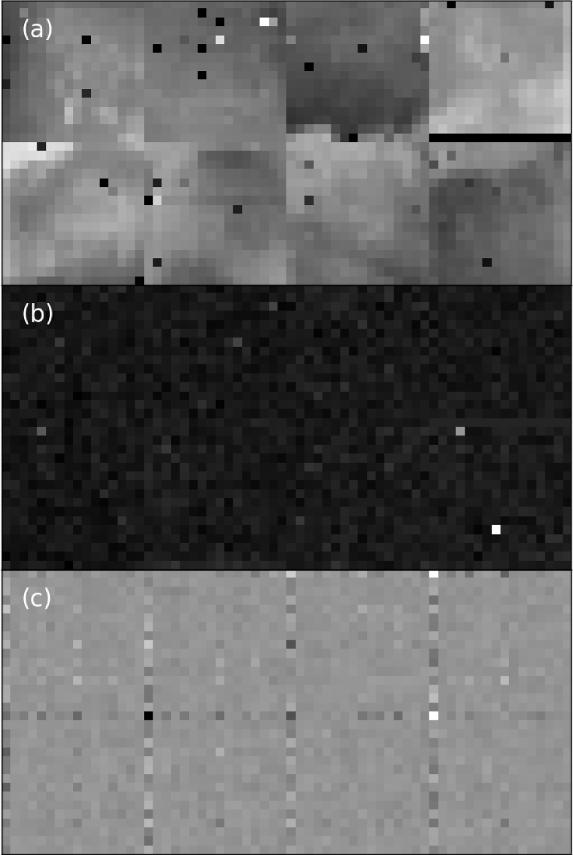
Figure 3: (a) Frame of the PACS imaging camera in the blue band. The darker and brighter isolated pixels are bad pixels. There is one complete bad line (at the bottom of the last matrix, ordered from the left to the right and from the bottom to the top). The observable structure is mainly the offset. Discontinuities in the offset correspond to the borders of the matrices of bolometers. Note that there are physical gaps between matrices as well as rotation and distortion. The matrix used in the transparent mode is the sixth one. (b) The same frame with the offset removed. The brighter isolated pixels are glitches. (c) The same frame after Hadamard transform. The offsets have not been removed.

Note that our method is not CS in a strict meaning. Because we have more data than unknowns, we cannot tell from the CS theory which compression matrix is optimal. But we think CS friendly compression matrices are worth being investigated as there is no other theory that point to other optimal compression matrices under sparsity assumptions. We plan to test a wider range of compression matrices in future works.

We also point out that the standard compression scheme of PACS scans (averaging) can also be modeled as in equation (9) replacing ${\mathb{C}}$ by an averaging matrix. The exact same inversion scheme can be applied to both the CS inversion problem and the standard inversion problem allowing a clear comparison by separating effects due to the acquisition matrix from those due to the sparsity constraint.

Equation (10) shows the averaging compression that is usually performed on PACS data. In this equation ${\mathb{I}}$ is the identity matrix of size the number of detectors.

$${\mathb{C}}_{AV}=\left(\begin{tabular}[]{ccccccc}{$\mathb{I}$}&\ldots&{$\mathb{I}$}&&&&\\ &&&$\ddots$&&&\\ &&&&{$\mathb{I}$}&\ldots&{$\mathb{I}$}\\ \end{tabular}\right)$$ (10)

Equation (11) shows the compressed-sensing compression that we implemented. ${\mathb{H}}$ is the Hadamard transform of one frame, and ${\mathb{M}}_{i}$ is a decimation matrix. A decimation matrix is a rectangular matrix with only ones and zeros values and exactly one non-zero element per row. It selects the elements of the Hadamard transform to be transmitted. For example, in the parallel mode, only one-eighth of the values are transmitted. The decimation matrices vary from one frame to the next to minimize the redundancy of the transmitted information. $F$ is the compression factor.

$$\small{\mathb{C}}_{CS}=\left(\begin{tabular}[]{ccccccc}${\mathb{M}}_{1}{\mathb{H}}$&&&&&&\\ &$\ddots$&&&&&\\ &&${\mathb{M}}_{F}{\mathb{H}}$&&&&\\ &&&${\mathb{M}}_{1}{\mathb{H}}$&&&\\ &&&&$\ddots$&&\\ &&&&&${\mathb{M}}_{F}{\mathb{H}}$&\\ \end{tabular}\right)$$ (11)

Note that all the matrices in this paper are not implemented as matrices but rather as linear functions as it would not be feasible to store such large matrices and prohibitive to perform matrix multiplications.

We define sparse priors in both wavelet space and finite difference. The criterion can then be rewritten as in equation (12), where ${\mathb{W}}$ is a wavelet transform and ${\mathb{D}}_{x}$ and ${\mathb{D}}_{y}$ are finite difference operators along both axes of the sky map. The finite difference operators simply compute the difference between two adjacent pixels along one axis or the other. Thus, as a prior they favor smooth maps. Since we minimize a $L_{1}$ norm, it allows for some bigger differences, hence the map can be piecewise smooth.

$$\hat{{\mathb{x}}}_{CSH} = \displaystyle\mathop{\mathrm{arg\,min}}_{{\mathb{x}}}{\|{\mathb{z}}-{\mathb{C}}{\mathb{P}}{\mathb{x}}\|^{2}}$$ (12)

$${}+\lambda_{W}\|{\mathb{W}}{\mathb{x}}\|_{1}+\lambda_{x}\|{\mathb{D}}_{x}{\mathb{x}}\|_{1}+\lambda_{y}\|{\mathb{D}}_{y}{\mathb{x}}\|_{1}$$

We estimate $\hat{{\mathb{x}}}_{CSH}$ (CSH meaning Compressed-Sensing for Herschel) using a conjugate gradient (CG) with Huber norm. The Huber norm is defined according to equation (13).

$$\left\{\begin{array}[]{cccc}\mathcal{H}(x)&=&x^{2}&,\forall x\in\left[-\delta,\delta\right]\\ \mathcal{H}(x)&=&2\left|\delta x\right|-\delta^{2}&,\forall x\notin\left[-\delta,\delta\right]\\ \end{array}\right.$$ (13)

The Huber norm is a way to approximate a L₁ norm ($\|\cdot\|_{1}$) with a function everywhere differentiable, which is mandatory in order to use CG methods. For this purpose, the Huber parameter $\delta$ can be chosen very small.

Finally, we minimize equation (14).

$$\hat{{\mathb{x}}}_{CSH} = \displaystyle\mathop{\mathrm{arg\,min}}_{{\mathb{x}}}{\|{\mathb{z}}-{\mathb{C}}{\mathb{P}}{\mathb{x}}\|^{2}}$$ (14)

$$+\lambda_{W}\mathcal{H}({\mathb{W}}{\mathb{x}})+\lambda_{x}\mathcal{H}({\mathb{D}}_{x}{\mathb{x}})+\lambda_{y}\mathcal{H}({\mathb{D}}_{y}{\mathb{x}})$$

This optimization scheme is very similar to Lustig et al. (2007) in the idea of applying CG iterations and replacing the L₁ norm by a close function everywhere differentiable.

5 Preprocessing

It is important to note that despite the significant alteration of the aspect of the data after CS compression (or any kind of linear compression), it is still possible to apply the same preprocessing steps that are performed in the standard PACS pipeline. Let us demonstrate this in details.

The following is usually applied to the data before the inversion step (back-projection or MADmap) :

• Removal of the offset by removing the temporal mean along each timeline

• Deglitching

• Pink noise filtering using median filtering (removes only the slowly drifting part in the case of MADmap)

5.1 Offset and pink noise removal

The removal of the offset is simple. Since the compression is linear, and applied independently on each frame, one can remove the offset by removing the temporal mean as in the averaging mode. The same applies for the pink noise removal.

In order to mitigate the effect of pink noise in the estimated maps, a filtering is performed during the preprocessing. Following the method of the pipeline, we use an high-pass median filtering. This can have a side effect of removing signal of interest at larger spatial scales in the map. This is of little importance in fields containing mostly point sources but can be dramatic in fields with structures at every scale such as fields taken in the galactic plane. One of the interests of MADmap is to be able to remove the pink noise artifacts in the maps without affecting the large scale structures. But even with MADmap-like methods, one still have to remove the very low frequency component of the pink noise not taken into account by the estimated noise covariance matrix. That is why it is important to ensure that one can perform median filtering in a CS framework.

We perform high-pass median filtering on the CS data exactly in the same way as it is done with the averaged data. Thanks to the linearity of the CS compression model, the pink noise in the raw data remains pink noise in the CS data. Thus, the median filtering affects the noise in the CS data the same way it does in the averaged data.

The only important parameter in the median filtering is the length of the sliding window used to compute the median in the neighborhood of each point. If the window is too large, there will be too much pink noise remaining in the filtered data. If it is too small, large scale structures in the map will start to get affected. As a compromise, we choose the window to be of the size of a scan leg, which is approximately the largest scale in the map. In the NGC6946 maps this corresponds very roughly to a window of 1000 samples at a sample rate of 40 Hz at a speed of 60 arcsec/s. For the compressed data, we divide this length by the compression factor.

5.2 Deglitching

The deglitching is more complicated since it makes use of spatial information. In order to apply deglitching in the CS case, we first decompress the data without projecting onto the sky map (equation (15)).

$$\hat{{\mathb{y}}}=({\mathb{C}}^{T}{\mathb{C}})^{-1}{\mathb{C}}^{T}{\mathb{z}}$$ (15)

We can then perform deglitching on $\hat{{\mathb{y}}}$ as we would have done on averaged data. We perform deglitching on $\hat{{\mathb{y}}}$ using a method called second level deglitching. It consists of regrouping all data samples that correspond to a given pixel map and masking out the ones that are beyond a given threshold using the median absolute deviation (MAD) method.

Note that any operation that is performed on standard data could be applied on CS data using equation (15). This is a very important advantage of using a linear compression method. Other compression methods, such as JPEG for instance, do not satisfy this property, since a thresholding is performed. It is also the linearity of the compression which allows to jointly perform the decompression and the map-making steps of the inversion and thus to obtain better maps.

When ${\mathb{C}}$ is an averaging matrix (the standard compression), the samples that are found to be glitches are simply masked. In our case, we define a masking matrix ${\mathb{M}}$ which is simply an identity matrix with zeros on diagonal elements corresponding to where values are masked. We can finally perform the inversion replacing ${\mathb{C}}{\mathb{P}}$ by ${\mathb{C}}{\mathb{M}}{\mathb{P}}$ in equation (14). This way, the inversion is done without altering the data set but entries corresponding to glitches are not taken into account in the inversion.

As can be seen in the maps in Figure 4, this is an effective method since no glitch remains visible. To ensure optimal detectability of the glitches it is best to perform pink noise removal beforehand. One can use a shorter window for the median filtering to better remove the pink noise only for the deglitching step. Indeed, in this case, it does not matter if the map structures are affected since the filtered data are only used to compute a mask for the glitches. One can then apply the mask on the data filtered with a larger window to preserve large scale structures.

5.3 Conclusion

To summarize, we can perform the same processing as the pipeline in the CS mode. There is no obstacle remaining which would prevent us from applying CS to PACS data. Let us see now the results we obtained with CS on real data.

6 Results

We present results of sky map estimation using PACS data observations in transparent mode. The different modes of compression are simulated. (PL) is the pipeline mode, i.e. a simple weighted backprojection ignoring that the data have been compressed (see equation 2). Compression is done by averaging. (PLI) is a full inversion of the pipeline model. It means it does not take into account the correct compression model. Data for (PLI) have been compressed by averaging. In other words (PLI) is the same as (PL) replacing the backprojection with a full inversion. (ACI) is the inversion of the model including the compression by averaging, (HCI) is the inversion with Hadamard compression and (NOC) is the inversion of the full data set (not compressed). All these methods but (PL) use the same sparse inversion algorithm described in section 4.2.

The compression factor on the acquisition side is always 8 in the following results except for the reference map (Figure 4e) for which no compression is applied. The data have been taken in fast scan mode (60 arcsec/s). Those are the conditions that give the most important loss of resolution in standard (averaging) mode since the blurring of each frame is the most important. The data set is made of two cross scans in the blue band of approximately 60000 frames each. Each frame has 256 pixels (instead of 2048 because of the transparent mode). The estimated map is made of $192\times 192$ pixels of 3 arcsec each, resulting in a 10 arcmin² map. The object observed is the galaxy NGC6946 from the KINGFISH program (P.I. R. Kennicutt) but the observations are dedicated calibration observations. Results are presented in Figure 4. Cuts along a line going through the two sources in the zoom are presented in Figure 5.

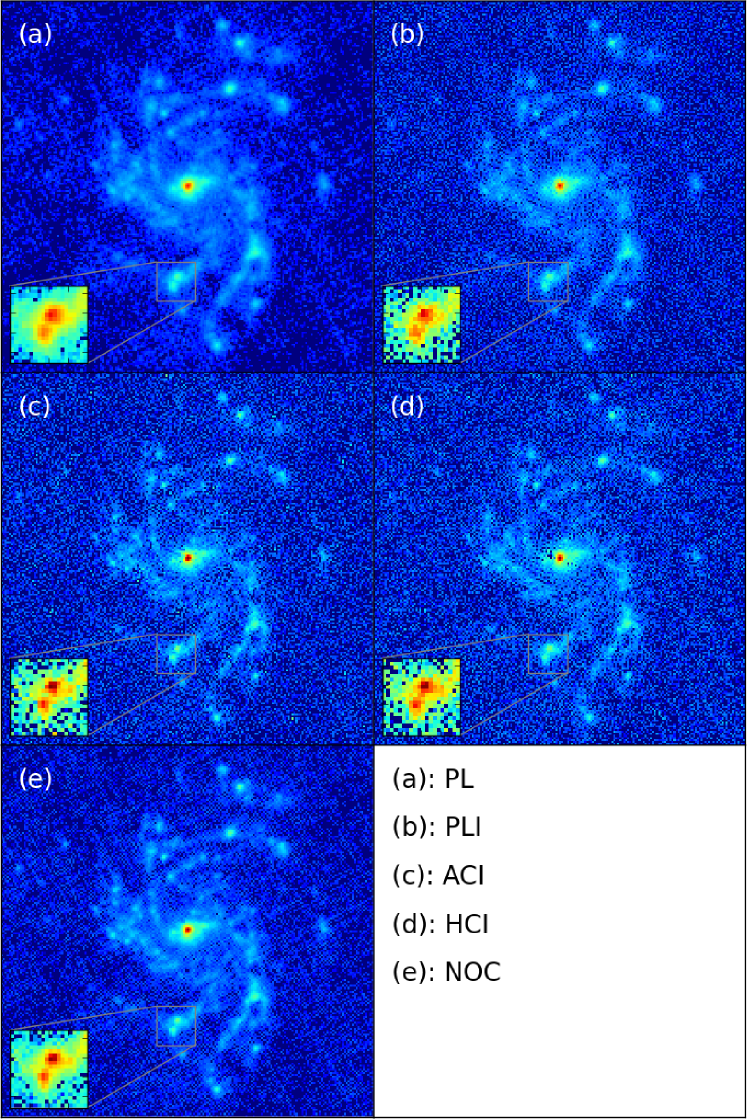
Figure 4: Map estimations of NGC 6946 using (a) the pipeline (PL) back-projection method , (b) the pipeline model inversion (PLI) (without taking into account the compression), (c) averaging compression inversion (ACI), (d) Hadamard compression inversion (HCI) and (e) reference map without any compression (NOC). Maps are presented on a fourth root intensity scale. All maps have the same scale.

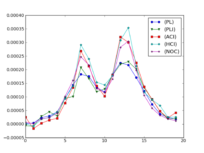
Figure 5: Line cuts along the two sources displayed in the zoom of figure 4. Cuts are made by two-dimensional linear interpolation of the maps. The x axis is the pixel index of the interpolation. The y axis is the intensity in Jy.

To illustrate the impact on the spatial resolution of the different reconstruction methods, we list in Table 2 the mean of the full width at half maximum (FWHM, in pixels) derived from Gaussian fits to four compact sources selected on the field. Although these sources are all not-strictly point-like, comparison of the achieved mean FWHM is quite instructive.

FWHM (pixels)	(PL)	(PLI)	(ACI)	(HCI)	(NOC)
mean of 4 sources	4.30	4.01	2.75	3.27	3.15

Table 2: FWHM of sources in pixels in Figure 4 estimated using 2-dimensional Gaussian fits of 4 isolated sources randomly chosen from the map.

To compare quantitatively the global results, we made radial profiles of NGC 6946 using maps from each method. Radial profiles were obtained using galaxy parameters from the NASA Extragalactic Database (NED) and summed up in Table 4. Surface brightness is averaged over pixels contained in concentric ellipses. Background values are estimated using corners of the maps where no source can be seen. The standard deviation of the pixels in the background areas give an estimate of the standard deviation of the noise in the whole map. Those values are reported in Table 3.

Maps	(PL)	(PLI)	(ACI)	(HCI)	(NOC)
std (10-6 Jy)	4.84	14.3	19.2	20.3	8.3

Table 3: Standard deviation for each map in Figure 4. Those values are estimated from the corners of the maps ($\sim$ 50 $\times$ 50 pixels area at each corner for a total of $\sim$ 10000 pixels in each map).

Results are presented in Figure 6. Figure 6a shows radial profiles corresponding to each map from figure 4. Those profiles are supplemented with error bars estimated from the background measurements given in Table 3. We assumed normal noise meaning that the standard deviation of the surface brightness at each radius is given by $\sigma_{profile}=\frac{\sigma_{bkg}}{\sqrt{N(r)}}$, where $N(r)$ is the number of pixels in at radius $r$ and $\sigma_{bkg}$ is the standard deviation of the pixels in the background.

Figure 6b shows the ratio of those radial profiles over the radial profile of the reference map without compression. Note that the reference map is not guaranteed to be the ground truth. In particular, it is affected with the potential issues of the median filtering (used to remove pink noise) as much as the other maps. However, we assume it is closer to the ground truth since it does not suffer from a loss of information due to compression.

We deduced the total flux of NGC6946 from the maps in Figure 4 and we display the result in Table 5.

PA (∘)	i (∘)	ra (∘)	dec (∘)
52.5	46	308.71	60.153

Table 4: Parameters of the NGC 6946 galaxy. PA is the position angle, i is the inclination, ra is the right ascension and dec is the declination.

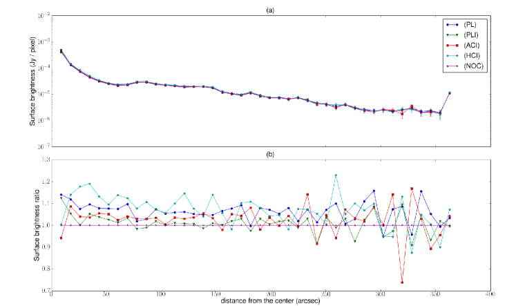
Figure 6: (a) Radial profiles of NGC 6946 in surface brightness (Jy) as a function of distance from the center of the galaxy (arcsec). Error bars are inferred from the background measurements reported in Table 3 and from the number of pixels at in the ellipses at each radius. (b) Ratio of radial profiles of the different maps over the radial profile of the reference map obtained without compression. Radial profiles are obtained from the maps in Figure 4. Acronyms refers to Figure 4.

Maps	(PL)	(PLI)	(ACI)	(HCI)	(NOC)
flux (Jy)	0.65	0.62	0.64	0.67	0.63

Table 5: Total flux of NGC 6946 in Jy as estimated from the maps of Figure 4.

7 Discussion

Comparing Figures 4a and 4b, there is a small gain in resolution. The FWHM estimate in table 2 illustrates this small gain since the FWHM drops from 4.3 pixels to 4.0 pixels. This gain comes from the inversion of the projection matrix. Physically, it means that we used the pointing information to get a super-resolved map. Note that this results holds only for the blue band which is not sampled at the Nyquist frequency.

Looking at Figure 4, maps ACI and HCI are better resolved than maps PL and PLI. This is supported by the quantitative results presented in Table 2. Figure 5 shows that this gain in resolution allows close sources to be better separated. From Table 2, the gain in resolution is approximately 1 pixel, or 3 arcseconds. This gain is due to the inversion of linear models which take into account the compression step and to the inclusion of sparsity priors in the inversion algorithm. This is common to both ACI and HCI and not intrinsic to CS.

Comparing ACI and HCI in Figure 4, it appears that the structure of the remaining noise is different. HCI does not exhibit linear patterns in the noise, following the scan direction. This is due to the mixing of the pink noise component of each detector done by the Hadamard compression. Furthermore, Table 2 shows that ACI has a mean FWHM below NOC. This is unexpected since NOC has more data than ACI. But this can be explained by the median filtering performed to filter the pink noise. Median filtering can have a small effect on compact sources even when large sliding windows are used. On the opposite, HCI seems more robust to this median filtering since the mean FWHM in the HCI map is just slightly above the NOC mean FWHM and not below it.

Of course, these lossy compression schemes still imply a loss of information but it mostly translates into an increase of the uncertainty of the map estimation (i.e. the noise). This is true for both compression matrices.

Note, however, that comparing results between CS and averaging compression matrices does not allow to conclude on the absolute performance of compressed-sensing. To conclude on this point, a study is needed to find the best CS compression matrix. In this paper we only try to highlight the applicability of CS methods to real data from a space observatory.

The amount of residual noise can seem surprising if one does not remember that the noise in PACS data is mostly a pink noise, and thus is not well taken into account in our inversion model. We need to make use of the noise covariance matrix in our inversion scheme. In order to do so, we can update equation (14) by taking into account a noise covariance matrix. This can be done using methods inspired by MADmap. We will investigate this possibility in a forthcoming article. However, since the resolution is increased in our results, the noise increase cannot be directly translated into a sensitivity decrease.

In figure (6a), we can see that the radial profiles obtained using the maps displayed in figure (4) are very close to each other. It gives confidence in the capability of our methods to preserve the flux in the maps at larger scales. In particular, this shows that the high-pass filtering is not affecting the profiles differently for CS than for averaging compression. It validates the way we perform this preprocessing step in the CS pipeline.

Figure (6b) shows the relative discrepancies between the profiles. They are higher further from the center since the surface brightness are very low, but they are consistent with the uncertainties. Again the CS compression scheme and the averaging compression scheme are very similar.

Profiles from compressed maps seem to be systematically slightly over-estimated between 0 and 150 arcseconds from the center, especially for (HCI) and (PL) maps. However, as shown in Table 5 the total flux of the galaxy computed for each map are within 7 % of the flux computed from the reference map. This result is in full accordance with the photometric accuracy quoted by the PACS team (Poglitsch et al., 2010).

We presented results for a resolved galaxy only but our method could benefit other objects. For example, deep survey observations are limited by the confusion limit at which the presence of numerous unresolved sources appear as noise. We plan to see if the confusion limit could be improved with our approach in future work. The gain in resolution could also help with regard to the source blending issue and could help improve the precision of catalogs of isolated unresolved sources (as estimated by SExtractor (Bertin & Arnouts, 1996), for instance). This could be tested on simulated field of sources with known positions. See also Pence et al. (2010) for a study on compression method using this idea.

8 Conclusions

In this paper we showed that methods inspired by the compressed-sensing theory can successfully be applied to real Herschel/PACS data, taking into account all the instrumental effects. For this purpose, special PACS data was acquired in the “transparent mode” in which no compression is applied. We then performed compressed-sensing compression scheme as well as the standard averaging compression scheme on the very same data which allows for an unbiased comparison. The data are affected by various artifacts such as pink noise and glitches. Handling of these artifacts is well known on standard averaged data but we show that the same kind of techniques can successfully be applied on compressed-sensing data.

Furthermore, we showed that it is possible to significantly improve the resolution in the sky maps compared to what can be obtained using the pipeline. This is done by taking into account the compression matrix in the acquisition model and by performing a proper inversion of the corresponding linear problem under sparsity constraints.

For now the resulting sky maps in CS and averaging compression modes are of the same quality. However, it is important to note that we may not be applying the best CS method. In particular, the Hadamard transform is only one compression matrix among others which satisfies the requirements for a CS application. Thus, this article does not in any way conclude on the performance of CS over standard compression. We can only conclude that this particular approach inspired by the CS framework and this particular Hadamard transform give as good results as the averaging compression matrix. But choosing another compression matrix could further improve the CS results over averaging.

We plan to more systematically analyse other choices for the compression matrix in a further article. Other improvements can be expected by performing deconvolution of the instrument PSF during the map-making stage and including the noise covariance matrix as in MADmap.

9 Acknowledgements

We thank the ASTRONET consortium for funding this work through the CSH and TAMASIS projects. Roland Ottensamer acknowledges funding by the Austrian Science Fund FWF under project number I163-N16.

References

- Bertin & Arnouts (1996) Bertin, E. & Arnouts, S. 1996, Astronomy and Astrophysics Supplement Series, 117, 393
- Bobin et al. (2008) Bobin, J., Starck, J., & Ottensamer, R. 2008, IEEE Journal of Selected Topics in Signal Processing, 2, 718
- Borer & Davies (2005) Borer, T. & Davies, T. 2005, EBU Technical Review, 303
- Bruckstein et al. (2009) Bruckstein, A., Donoho, D., & Elad, M. 2009, SIAM review, 51, 34
- Candès (2006) Candès, E. 2006, in Proceedings of the International Congress of Mathematicians, Vol. 3, Citeseer, 14331452
- Candès (2008) Candès, E. 2008, Comptes Rendus Mathematique, 346, 589
- Candès & Wakin (2008) Candès, E. & Wakin, M. 2008
- Candes & Wakin (2008) Candes, E. & Wakin, M. 2008, IEEE Signal Processing Magazine, 25, 21
- Cantalupo et al. (2010) Cantalupo, C., Borrill, J., Jaffe, A., Kisner, T., & Stompor, R. 2010, The Astrophysical Journal Supplement Series, 187, 212
- Chanial (2010) Chanial, P. 2010, in prep.
- de Graauw et al. (2010) de Graauw, T., Helmich, F. P., Phillips, T. G., et al. 2010, A&A, 518, L6+
- Donoho (2006) Donoho, D. 2006, IEEE Transactions on Information Theory, 52, 1289
- Griffin et al. (2010) Griffin, M. J., Abergel, A., Abreu, A., et al. 2010, A&A, 518, L3+
- Lustig et al. (2007) Lustig, M., Donoho, D., & Pauly, J. 2007, Magnetic Resonance in Medicine, 58, 1182
- Ottensamer & Kerschbaum (2008) Ottensamer, R. & Kerschbaum, F. 2008, in Presented at the Society of Photo-Optical Instrumentation Engineers (SPIE) Conference, Vol. 7019, Society of Photo-Optical Instrumentation Engineers (SPIE) Conference Series
- Pence et al. (2010) Pence, W. D., White, R. L., & Seaman, R. 2010, PASP, 122, 1065
- Pilbratt et al. (2010) Pilbratt, G. L., Riedinger, J. R., Passvogel, T., et al. 2010, A&A, 518, L1+
- Poglitsch et al. (2010) Poglitsch, A., Waelkens, C., Geis, N., et al. 2010, ArXiv e-prints
- Pratt et al. (1969) Pratt, W., Kane, J., & Andrews, H. 1969, Proceedings of the IEEE, 57, 58
- Skodras et al. (2001) Skodras, A., Christopoulos, C., & Ebrahimi, T. 2001, IEEE signal processing magazine, 18, 36
- Starck et al. (2010) Starck, J.-L., Murtagh, F., & Fadili, M. 2010, Sparse Image and Signal Processing (Cambridge University Press)
- Stojnic et al. (2008) Stojnic, M., Xu, W., & Hassibi, B. 2008, in IEEE International Symposium on Information Theory, 2008. ISIT 2008, 2182–2186