Black p-Branes versus black holes in non-asymptotically flat Einstein-Yang-Mills theory

Abstract

We present a class of non-asymptotically flat (NAF) charged black p-branes (BpB) with p-compact dimensions in higher dimensional Einstein-Yang-Mills theory. Asymptotically the NAF structure manifests itself as an anti-de-sitter spacetime. We determine the total mass / energy enclosed in a thin-shell located outside the event horizon. By comparing the entropies of BpB with those of black holes in same dimensions we derive transition criteria between the two types of black objects. Given certain conditions satisfied our analysis shows that BpB can be considered excited states of black holes. An event horizon $r_{+}$ versus charge square $Q^{2}$ plot  for the BpB reveals such a transition where $r_{+}$ is related to the horizon radius $r_{h}$ of the black hole (BH) both with the common charge $Q.$

I Introduction

It is well-known that by uplifting $d-$dimensional dilatonic black holes (BH) one obtains $\left(d+p\right)-$dimensional black $p-$branes (BpB) with extended event horizons 1 ; 2 ; 3 ; 4 . A black string (BS), for $p=1$ is an extension with one extra dimension whose horizon has a product topology such as $R\times S^{d-2}$. Naturally the simplest member of this class constitutes the chargeless Schwarzschild metric in $d=4$ and $p=1$, so that the topology becomes $R\times S^{2}$ 5 ; 6 . In case that the extra dimension is compact the end points may be identified to give a BS with horizon topology $S^{1}\times S^{2}$. Concerning BS (and more generally BpB) an interesting problem that gave birth to a considerable literature in recent years is their instability against decay into BH (or vice versa). This problem was pointed out first, through perturbation analysis by Gregory and Laflamme (GL) which came to be known as GL instability 7 ; 8 . Such a perturbative stability / instability applies to asymptotically flat (AF) metrics, which should not be reliable for non-asymptotically flat (NAF) spacetimes. Both for magnetic 9 ; 10 and electric charges 11 the GL instability has been shown perturbatively in AF spacetimes to remain intact.

In this paper we employ local thermodynamical stability / instability arguments supplemented with entropy comparison to relate charged BpB and BH in NAF spacetimes. In doing this we assume that both, the charges and the Hawking temperatures of BpB and BH are same. Our system consists of $d-$dimensional Einstein-Yang-Mills (EYM) theory in a compact $p-$dimensional brane world which admits NAF black objects. Among a large class of BH solutions which can be used to generate a family of BpB we choose a specific BH solution so that technically it becomes tractable. In other words, as long as the NAF condition is assumed the freedom of alternative solutions is always available. Our line element has the particular property that the coefficient of the angular part, i.e. $d\Omega_{d-2}^{2}$ is a constant. Non-Abelian gauge fields were considered as BS solutions by other researchers 12 ; 13 ; 14 ; 15 . Our approach, however, differs from other studies where we present exact non-Abelian solutions in all dimensions. Asymptotically our solutions represent anti-de Sitter (AdS) spacetimes. Further, by assuming an imaginary thin-shell of finite radius ($r=r_{B}$) as boundary outside the horizon, we determine the total energy as $r_{B}\rightarrow\infty.$ For $d>4,$ however, the mass of our NAF black hole diverges as $r_{B}\rightarrow\infty.$ This has been adopted as a useful technique to define mass in NAF metrics of general relativity 16 ; 17 . Herein we wish to follow the same trend. This reflects the fundamental difficulty in defining total mass for a NAF metric.  We resort next to compare the entropies of BpB and BH with related horizons $r_{+}$ and $r_{h},$ respectively, but with the common charge $Q$. The equality of charges can easily be justified as the conservation of charge whereas the relation between horizon radii of the two species is obtained from the equality of their Hawking temperatures. From comparison of entropy expressions we plot $r_{+}$ versus $Q^{2}$ for $5\leq d+p\leq 10$ to identify the regions of both BpB and BH. The intersecting curve determines naturally the transition between BpB to BH and vice versa. The figure implies that for a given dimension $d+p=$ constant, increasing $p$ / decreasing $d,$ favors a larger region for BH/ BpB. Assuming any relation between the charges of BH and BpB will naturally give rise to a geometrical constraint between two structures that undergo transition with the mass calculation in a thin-shell formalism. Organization of the paper is as follows.

In section II we present our exact EYM solutions in all dimensions. Thermodynamic stability of the solution is discussed in section III. We summarize our results in Conclusion which appears in section IV.

II The NAF EYM solution

Our $(d+p)-$dimensional action with $p-$compact dimensions in EYM theory is given by

$$I=\frac{1}{16\pi G_{\left(d+p\right)}^{BpB}}\int_{0}^{L_{p}}dz_{p}...\int_{0}^{L_{1}}dz_{1}\int d^{d}x\sqrt{-g}\left(R-\mathcal{F}\right)$$ (1)

in which

$$\mathcal{F}=\mathbf{Tr}(F_{\mu\nu}^{\left(a\right)}F^{\left(a\right)\mu\nu})$$ (2)

and

$$\mathbf{F}^{\left(a\right)}=\mathbf{dA}^{\left(a\right)}+\frac{1}{2\sigma}C_{\left(b\right)\left(c\right)}^{\left(a\right)}\mathbf{A}^{\left(b\right)}\wedge\mathbf{A}^{\left(c\right)},$$ (3)

is the YM $2-$form field with structure constants $C_{\left(b\right)\left(c\right)}^{\left(a\right)}.$ Here $R$ is the Ricci scalar, the coupling constant $\sigma$ is expressed in terms of the YM charge and

$$\mathbf{Tr}(.)=\sum\limits_{a=1}^{\frac{\left(d-1\right)(d-2)}{2}}\left(.\right).$$ (4)

Note that $G_{\left(d+p\right)}^{BpB}$ represents the $d+p-$dimensional Newton constant while $L_{i}$ ($1\leq i\leq p$) stands for a set of compact dimensions. We note also that $L_{i}=L,$ for all $1\leq i\leq p,$ need not to be assumed here. For future reference we prefer to use $L_{i}\neq L_{j}$ for $i\neq j$ in this paper. As a matter of fact our results in this paper will be valid irrespective of the compact volume. Our ultimate choice in this study will be $\prod\limits_{i=1}^{p}L_{i}=1,$ so that if $L_{i}=\epsilon$ and $L_{j}=\frac{1}{\epsilon},$ for some $i$ and $j$ and $\epsilon\rightarrow 0$ we preserve the same volume with non-compact translational symmetry. Our pure magnetic YM potential follows from the higher dimensional version 18 ; 19 ; 20 ; 21 ; 22 of the Wu-Yang ansatz which is given by

$$\mathbf{A}^{(a)} =\frac{Q}{r^{2}}C_{\left(i\right)\left(j\right)}^{\left(a\right)}\ x^{i}dx^{j},\text{ \ \ }Q=\text{YM magnetic charge, \ }r^{2}=\overset{d-1}{\underset{i=1}{\sum}}x_{i}^{2},$$ (5)

$$2 \leq j+1\leq i\leq d-1,\text{ \ and \ }1\leq a\leq\left(d-1\right)(d-2)/2,$$

$$x_{1} =r\cos\theta_{d-3}\sin\theta_{d-4}...\sin\theta_{1},\text{ }x_{2}=r\sin\theta_{d-3}\sin\theta_{d-4}...\sin\theta_{1},$$

$$\text{ }x_{3} =r\cos\theta_{d-4}\sin\theta_{d-5}...\sin\theta_{1},\text{ }x_{4}=r\sin\theta_{d-4}\sin\theta_{d-5}...\sin\theta_{1},$$ (6)

$$...$$

$$x_{d-2} =r\cos\theta_{1}.$$

The associated Lie group for the YM field is $SO(N-1)$ whereas the group of motion over $p-$branes is the Euclidean $E^{P}.$ The overall product group becomes therefore $E^{P}\times SO\left(N-1\right)$. Our choice for the BpB metric ansatz is given by

$$ds^{2} = e^{-b\psi}\left(-f\left(r\right)dt^{2}+\frac{dr^{2}}{f\left(r\right)}+h\left(r\right)^{2}d\Omega_{\left(d-2\right)}^{2}\right)+e^{\frac{b\left(d-2\right)}{p}\psi}dz^{i}dz^{i},$$

$$\left(i=1,2,...,p\right)\text{ }(b=\text{constant})$$

in which $\psi\left(r\right),$ $f\left(r\right)$ and $h\left(r\right)$ are metric functions of $r$ to be found and $d\Omega_{\left(d-2\right)}^{2}$ is the $\left(d-2\right)-$dimensional unit spherical line element. Herein, $b$ is a constant scaling for $\psi\left(r\right)$ that plays role in going from lower to higher dimensions or vice versa. We note that $b=0$, smears out the function $\psi\left(r\right)$ as well which reduces the line element (6) to the case of AF-BpB. For this reason from the outset we assume that the constant parameter $b$ takes values in the range $0<b<\infty$. In the sequel $b$ will be fixed in terms of other parameters. Variation of the action with respect to $g_{\mu\nu}$ yields

$$G_{\mu}^{\nu}=T_{\mu}^{\nu},$$ (8)

where

$$T_{\mu}^{\nu}=2\left[\mathbf{Tr}\left(F_{\mu\lambda}^{\left(a\right)}F^{\left(a\right)\nu\lambda}\right)-\frac{1}{4}\mathcal{F}\delta_{\mu}^{\nu}\right]$$ (9)

or explicitly

$$T_{\mu}^{\nu}=-\frac{\left(d-3\right)\left(d-2\right)Q^{2}}{2h^{4}}e^{2b\psi}\text{diag}\left[1,1,\overset{d-2-times}{\overbrace{\kappa,\kappa,...,\kappa}},\overset{p-times}{\overbrace{1,1,...,1}}\right],\text{ \ \ \ \ \ \ }\kappa=\frac{d-6}{d-2}$$ (10)

and non-zero $G_{\mu}^{\nu}$ are given by

$$\begin{tabular}[]{l}$G_{t}^{t}=\frac{\left(d-2\right)e^{b\psi}}{2h^{2}}\left[\frac{d+p-2}{4p}b^{2}fh^{2}\psi^{\prime 2}+hh^{\prime}f^{\prime}+2fhh^{\prime\prime}+\left(d-3\right)\left(fh^{\prime 2}-1\right)\right]$\end{tabular},$$ (12)

$$\begin{tabular}[]{l}$G_{r}^{r}=\frac{\left(d-2\right)e^{b\psi}}{2h^{2}}\left[-\frac{d+p-2}{4p}b^{2}fh^{2}\psi^{\prime 2}+hh^{\prime}f^{\prime}+\left(d-3\right)\left(fh^{\prime 2}-1\right)\right]$\end{tabular},$$ (14)

$$\begin{tabular}[]{l}$G_{\theta_{i}}^{\theta_{i}}=\frac{e^{b\psi}}{h^{2}}\left[\frac{d+p-2}{4p}\left(\frac{\left(d-2\right)}{2}b^{2}fh^{2}\psi^{\prime 2}\right)+\left(d-3\right)h\left(h^{\prime}f\right)^{\prime}+\frac{\left(d-3\right)\left(d-4\right)}{2}\left(fh^{\prime 2}-1\right)+\frac{1}{2}h^{2}f^{\prime\prime}\right]$\end{tabular},$$ (16)

$$\begin{tabular}[]{l}$G_{z_{i}}^{z_{i}}=\frac{\left(d-2\right)e^{b\psi}}{2h^{2}}\left[\frac{d+p-2}{4p}\left(b^{2}fh^{2}\psi^{\prime 2}-\frac{4b\left(f\psi^{\prime}\right)^{\prime}h^{2}}{\left(d-2\right)}-4hfb\psi^{\prime}h^{\prime}\right)+\frac{h^{2}f^{\prime\prime}}{d-2}+2h\left(h^{\prime}f\right)^{\prime}+\left(d-3\right)\left(fh^{\prime 2}-1\right)\right]$\end{tabular}.$$ (18)

The YM equations also follow from the action as

$$\mathbf{d}\left({}^{\star}\mathbf{F}^{\left(a\right)}\right)+\frac{1}{\sigma}C_{\left(b\right)\left(c\right)}^{\left(a\right)}\mathbf{A}^{\left(b\right)}\wedge^{\star}\mathbf{F}^{\left(c\right)}=0$$ (19)

where the hodge star ^⋆ implies duality. By direct substitution, one can show that YM equations are satisfied. Since this has been given elsewhere 18 ; 19 ; 20 ; 21 ; 22 it will not be repeated here. From $T_{t}^{t}=T_{r}^{r}$ (or $G_{t}^{t}=G_{r}^{r}$) it follows that

$$\frac{\left(d+p-2\right)b^{2}}{4p}\psi^{\prime 2}=-\frac{h^{\prime\prime}}{h},$$ (20)

which after setting $h=\xi e^{\alpha\psi}$ we obtain

$$\psi=\frac{\alpha}{\alpha^{2}+\left(\frac{d+p-2}{4p}\right)b^{2}}\ln\left(\xi_{1}r+\xi_{2}\right).$$ (21)

Here $\alpha$ is a parameter to be fixed while $\xi_{1}$and $\xi_{2}$ are two integration constants. Note also that we exclude the case $p=0$ so that the present class of black holes doesn’t admit previously known class such as Tangherlini 23 Technically we are interested in NAF solutions, we make the choice $\xi_{1}=1$ and $\xi_{2}=0$ and consequently

$$\psi=\frac{\alpha\ln r}{\alpha^{2}+\left(\frac{d+p-2}{4p}\right)b^{2}}.$$ (22)

Next, we substitute $\psi$ and $h$ into the EYM BpB equations (8) and upon the choice of $\alpha=\frac{b}{2},$ the field equations are all satisfied with

$$f\left(r\right)=\Xi\left(1-\left(\frac{r_{+}}{r}\right)^{\frac{\left(p+1\right)\left(d-2\right)}{d+2p-2}}\right)r^{\frac{2\left(d+p-2\right)}{d+2p-2}},$$ (23)

where

$$\Xi=\frac{\left(d-3\right)\left(d+p-2\right)}{Q^{2}\left(d-2\right)\left(p+1\right)}$$ (24)

and from $h=\xi e^{\alpha\psi},$ $\xi^{2}$ is determined as

$$\xi^{2}=\frac{Q^{2}\left(d+2p-2\right)}{d+p-2}.$$ (25)

Here $r_{+}$ is an integration constant which represents the radius of the event horizon and we also remark that for meaningful metric functions we must have $d>3$. Upon rewriting the line element in the form

$$ds^{2}=-f_{1}\left(r\right)dt^{2}+\frac{dr^{2}}{f_{2}\left(r\right)}+f_{3}\left(r\right)dz_{i}dz^{i}+f_{4}\left(r\right)d\Omega_{\left(d-2\right)}^{2}$$ (26)

the metric functions take the following forms

$$f_{1}\left(r\right) = f\left(r\right)e^{-b\psi}=\Xi\left(1-\left(\frac{r_{+}}{r}\right)^{\frac{\left(p+1\right)\left(d-2\right)}{d+2p-2}}\right)r^{\frac{2\left(d-2\right)}{d+2p-2}},$$ (27)

$$f_{2}\left(r\right) = f\left(r\right)e^{b\psi}=\Xi\left(1-\left(\frac{r_{+}}{r}\right)^{\frac{\left(p+1\right)\left(d-2\right)}{d+2p-2}}\right)r^{2},$$ (28)

$$f_{3}\left(r\right) = e^{\frac{b\left(d-2\right)}{p}\psi}=r^{\frac{2\left(d-2\right)}{d+2p-2}},\text{ \ \ \ }f_{4}\left(r\right)=e^{-b\psi}h\left(r\right)^{2}=\xi^{2},$$ (29)

and

$$h\left(r\right)=\xi r^{\frac{p}{d+2p-2}}.$$ (30)

We wish now to determine the total energy for a NAF metric enclosed in an imaginary thin-shell of radius $r=r_{B}$, where $r_{B}$ lies outside the event horizon ($r_{B}>r_{+}$). For this purpose we consider a timelike hypersurface $\Sigma$ defined by

$$r=r_{B}.$$ (31)

where $r_{B}$ is the radius of the hypersurface which we call, the boundary. By considering the constraint

$$-f_{1}\left(r\right)dt^{2}+\frac{dr^{2}}{f_{2}\left(r\right)}=-d\tau^{2}$$ (32)

in which $\tau$ is the proper time on the hypersurface, the line element on $\Sigma$ becomes

$$ds_{\Sigma}^{2}=-d\tau^{2}+f_{3}\left(r_{B}\right)dz_{i}dz^{i}+f_{4}\left(r_{B}\right)d\Omega_{\left(d-2\right)}^{2}.$$ (33)

In terms of the original coordinates $x^{\gamma}=\left(t,r,z_{1},z_{2},...,\theta_{1},\theta_{2},...\right)$ the induced metric $\xi^{i}=\left(\tau,z_{1},z_{2},...,\theta_{1},\theta_{2},...\right)$ on $\Sigma$ is given by (Latin indices run over the induced coordinates and Greek indices run over the original manifold’s coordinates)

$$g_{ij}=\frac{\partial x^{\alpha}}{\partial\xi^{i}}\frac{\partial x^{\beta}}{\partial\xi^{j}}g_{\alpha\beta}.$$ (34)

Here

$$g_{ij}=\text{diag}\left(-1,f_{3}\left(r_{B}\right),f_{3}\left(r_{B}\right),...,f_{4}\left(r_{B}\right),f_{4}\left(r_{B}\right),...\right),$$ (35)

while the extrinsic curvature is defined by

$$K_{ij}=-n_{\gamma}\left(\frac{\partial^{2}x^{\gamma}}{\partial\xi^{i}\partial\xi^{j}}+\Gamma_{\alpha\beta}^{\gamma}\frac{\partial x^{\alpha}}{\partial\xi^{i}}\frac{\partial x^{\beta}}{\partial\xi^{j}}\right)_{r=r_{B}}.$$ (36)

It is assumed that $\Sigma$ is timelike, whose unit $\left(d+p\right)-$normal in $M$ is given by

$$n_{\gamma}=\left(-\left|g^{\alpha\beta}\frac{\partial F}{\partial x^{\alpha}}\frac{\partial F}{\partial x^{\beta}}\right|^{-1/2}\frac{\partial F}{\partial x^{\gamma}}\right)_{r=r_{B}},$$ (37)

in which $F$ is the equation of the hypersurface $\Sigma,$ i.e.

$$F\left(r\right)=r-r_{B}=0.$$ (38)

From the Lanczos equation 24 ; 25 ; 26 (this is the Einstein equation on the hypersurface) the intrinsic surface stress–energy tensor, $S_{i}^{j}=$diag$\left(-\sigma,p_{\theta_{1}},p_{\theta_{2}},...\right)$, is given by

$$S_{i}^{j}=-\frac{1}{8\pi G_{\left(d+p\right)}^{BpB}}\left(K_{i}^{j}-K\delta_{i}^{j}\right),$$ (39)

in which $K$ is the trace of $K_{i}^{j}.$

Applying the above equations leads to

$$g^{\alpha\beta}\frac{\partial F}{\partial x^{\alpha}}\frac{\partial F}{\partial x^{\beta}}=g^{rr}\left(\frac{\partial F}{\partial r}\right)^{2}=g^{rr}=f_{2}\left(r_{B}\right)$$ (40)

and therefore

$$n_{\gamma}=-\frac{1}{\sqrt{f_{2}\left(r_{B}\right)}}\frac{\partial F}{\partial x^{\gamma}}=-\frac{1}{\sqrt{f_{2}\left(r_{B}\right)}}\left(0,1,0,0,...\right).$$ (41)

This helps us to find

$$K_{\tau}^{\tau}=-\frac{\sqrt{f_{2}\left(r_{B}\right)}}{2}\frac{f_{1}^{\prime}\left(r_{B}\right)}{f_{1}\left(r_{B}\right)}$$ (42)

$$K_{z_{i}}^{z_{i}}=-\frac{\sqrt{f_{2}\left(r_{B}\right)}}{2}\frac{f_{3}^{\prime}\left(r_{B}\right)}{f_{3}\left(r_{B}\right)}$$ (43)

$$K_{\theta_{i}}^{\theta_{i}}=-\frac{\sqrt{f_{2}\left(r_{B}\right)}}{2}\frac{f_{4}^{\prime}\left(r_{B}\right)}{f_{4}\left(r_{B}\right)},$$ (44)

and consequently

$$K=K_{i}^{i}=-\frac{\sqrt{f_{2}\left(r_{B}\right)}}{2}\frac{f_{1}^{\prime}\left(r_{B}\right)}{f_{1}\left(r_{B}\right)}-\frac{p\sqrt{f_{2}\left(r_{B}\right)}}{2}\frac{f_{3}^{\prime}\left(r_{B}\right)}{f_{3}\left(r_{B}\right)}-\frac{\left(d-2\right)\sqrt{f_{2}\left(r_{B}\right)}}{2}\frac{f_{4}^{\prime}\left(r_{B}\right)}{f_{4}\left(r_{B}\right)}.$$ (45)

The energy density $\sigma$ on the boundary and pressure $p_{i}$ are as follow

$$\sigma=-S_{\tau}^{\tau}=\frac{1}{8\pi G_{\left(d+p\right)}^{BpB}}\left(\frac{p\sqrt{f_{2}\left(r_{B}\right)}}{2}\frac{f_{3}^{\prime}\left(r_{B}\right)}{f_{3}\left(r_{B}\right)}+\frac{\left(d-2\right)\sqrt{f_{2}\left(r_{B}\right)}}{2}\frac{f_{4}^{\prime}\left(r_{B}\right)}{f_{4}\left(r_{B}\right)}\right),$$ (46)

$$p_{\theta_{i}}=\frac{1}{8\pi G_{\left(d+p\right)}^{BpB}}\left(-\frac{\sqrt{f_{2}\left(r_{B}\right)}}{2}\frac{f_{1}^{\prime}\left(r_{B}\right)}{f_{1}\left(r_{B}\right)}-\frac{p\sqrt{f_{2}\left(r_{B}\right)}}{2}\frac{f_{3}^{\prime}\left(r_{B}\right)}{f_{3}\left(r_{B}\right)}-\frac{\left(d-3\right)\sqrt{f_{2}\left(r_{B}\right)}}{2}\frac{f_{4}^{\prime}\left(r_{B}\right)}{f_{4}\left(r_{B}\right)}\right),$$ (47)

$$p_{z_{i}}=\frac{1}{8\pi G_{\left(d+p\right)}^{BpB}}\left(-\frac{\sqrt{f_{2}\left(r_{B}\right)}}{2}\frac{f_{1}^{\prime}\left(r_{B}\right)}{f_{1}\left(r_{B}\right)}-\frac{\left(p-1\right)\sqrt{f_{2}\left(r_{B}\right)}}{2}\frac{f_{3}^{\prime}\left(r_{B}\right)}{f_{3}\left(r_{B}\right)}-\frac{\left(d-2\right)\sqrt{f_{2}\left(r_{B}\right)}}{2}\frac{f_{4}^{\prime}\left(r_{B}\right)}{f_{4}\left(r_{B}\right)}\right).$$ (48)

In order to find the total energy (=Mass), we use the following integral

$$\Omega=\int\sqrt{-g}\left(\rho+p_{r}\right)d^{d+p}x$$ (49)

in which $p_{r}$ is the radial pressure. For the boundary surface we have $p_{r}=0$ and $\rho=\sigma\delta\left(r-r_{B}\right)$ where $\delta\left(r-r_{B}\right)$ stands for the Dirac delta function. A simple calculation results in (keeping in mind that each $z_{i}$ is compact and contributes trivially)

$$\Omega = \int\limits_{0}^{L_{p}}...\int\limits_{0}^{L_{1}}\int\limits_{0}^{2\pi}\int\limits_{0}^{\pi}...\int\limits_{0}^{\pi}\int\limits_{0}^{\infty}\sqrt{-g}\sigma\delta\left(r-r_{B}\right)drd\theta_{1}...d\theta_{d-2}dz_{1}...dz_{p}=$$

$$\frac{\pi^{\frac{d-1}{2}}\prod\limits_{k=1}^{p}L_{k}}{8\pi\Gamma\left(\frac{d-1}{2}\right)G_{\left(d+p\right)}^{BpB}}\sqrt{f_{1}\left(r_{B}\right)f_{3}\left(r_{B}\right)^{p}f_{4}\left(r_{B}\right)^{d-2}}\left(p\frac{f_{3}^{\prime}\left(r_{B}\right)}{f_{3}\left(r_{B}\right)}+\left(d-2\right)\frac{f_{4}^{\prime}\left(r_{B}\right)}{f_{4}\left(r_{B}\right)}\right).$$

In terms of our metric functions one finds

$$\Omega=\frac{\pi^{\frac{d-1}{2}}\xi^{d-2}\sqrt{\Xi}\prod\limits_{k=1}^{p}L_{k}}{4\pi\Gamma\left(\frac{d-1}{2}\right)G_{\left(d+p\right)}^{BpB}}\frac{\left(d-2\right)p}{d+2p-2}\frac{1}{r_{B}}\left(1-\left(\frac{r_{+}}{r_{B}}\right)^{\frac{\left(p+1\right)\left(d-2\right)}{d+2p-2}}\right)^{1/2}r_{B}^{\frac{\left(d-2\right)\left(p+1\right)}{d+2p-2}},$$ (51)

which is in our case the total energy of the spacetime stored inside $r=r_{B}.$ One may call it the mass of the solution. In the case of $\left(4+p\right)-$dimensions we find

$$M=\Omega=\frac{1}{G_{\left(d+p\right)}^{BpB}}\sqrt{\frac{p^{2}Q^{2}}{2\left(d+2\right)\left(p+1\right)}}\prod\limits_{k=1}^{p}L_{k}\left(1-\frac{r_{+}}{r_{B}}\right)^{1/2},$$ (52)

which in the limit of $r_{B}\rightarrow\infty$ becomes

$$M=\frac{1}{G_{\left(d+p\right)}^{BpB}}\sqrt{\frac{p^{2}Q^{2}}{2\left(d+2\right)\left(p+1\right)}}\prod\limits_{k=1}^{p}L_{k},$$ (53)

and is finite. We admit, however, that for $d>4$ (with $p=$arbitrary) the mass expression (47) diverges when $r_{B}\rightarrow\infty.$ In order to understand the physical implication of this class of NAF solutions we investigate their asymptotic behaviors for $r\gg r_{+}$. For this purpose we make the transformation

$$r \rightarrow r^{-k}$$

$$\text{(}k = \frac{d+2p-2}{d-2}\text{),}$$ (54)

followed by the scalings

$$t \rightarrow \left(\frac{\Xi}{k}\right)t,$$

$$z_{i} \rightarrow \left(\frac{\sqrt{\Xi}}{k}\right)z_{i}$$ (55)

to yield for $r\gg r_{+}$

$$ds^{2}\simeq\frac{1}{r^{2}}\left(-dt^{2}+dr^{2}+dz_{i}dz^{i}\right)+\frac{d-3}{k\left(p+1\right)}d\Omega_{\left(d-2\right)}^{2}.$$ (56)

This is the geometry of the $(p+2)-$dimensional anti-de Sitter (AdS) spacetime times the $(d-2)-$dimensional sphere (i.e. $AdS_{p+2}\times S^{d-2}$). In analogy, near the horizon, i.e., $r=r_{+}+x$ with $x>0,$ ($x^{2}\approx 0$) we have our line element

$$ds^{2}\simeq-C_{0}xdt^{2}+\frac{dx^{2}}{C_{1}x}+C_{2}dz_{i}dz^{i}+\xi^{2}d\Omega_{\left(d-2\right)}^{2}$$ (57)

for appropriate constants $C_{i}.$ Applying now

$$x=\frac{1}{4}C_{1}y^{2}$$ (58)

and rescaling the time coordinate casts the metric into

$$ds^{2}\simeq-y^{2}d\bar{t}^{2}+dy^{2}+C_{2}dz_{i}dz^{i}+\xi^{2}d\Omega_{\left(d-2\right)}^{2}$$ (59)

which is the accelerated (Rindler) frame at the ($\bar{t},y$) (or $t,r$) sector. This is a product space of $2-$dimensional flat space with $p-$torus and $\left(d-2\right)-$dimensional sphere (i.e., $M^{2}\times T^{p}\times S^{d-2}$). From the general solution (23-26), for certain values of ($d,p$) we find the Ricci scalar ($R$) and Kretschmann scalar ($K$) as follow

$$d=4,\text{ \ }p=1,\text{ \ }R=\frac{3}{4Q^{2}},\text{ \ }K=\frac{171}{64Q^{4}},$$ (60)

$$d=4,\text{ \ }p=2,\text{ \ }R=\frac{4}{9Q^{2}},\text{ \ }K=\frac{16}{243Q^{4}}\left(29+\left(\frac{r_{+}}{r}\right)^{2}\right),$$ (61)

$$d=5,\ p=1,\ R=\frac{3}{4Q^{2}},\ K=\frac{6528}{625Q^{4}},\text{ \ \ }...\text{ .}$$ (62)

One characteristic feature of this class of solutions is that whenever $p=1$, irrespective of $d$, we have a regular solution while for $p>1$ it is singular at $r=0$.

The simplest member in this class of solutions is given by the choice $d=4,p=1$. This yields the line element of a black string 27

$$ds^{2}=-\frac{3\left(r-r_{+}\right)}{4Q^{2}}dt^{2}+\frac{4Q^{2}}{3r\left(r-r_{+}\right)}dr^{2}+rdz^{2}+\frac{4Q^{2}}{3}d\Omega_{2}^{2}$$ (63)

which is non-singular and manifestly NAF. The scalar curvature is $R=\frac{3}{8Q^{2}}$, and the Kretschmann scalar is $K=\frac{171}{64Q^{4}}$. From our foregoing argument this asymptotes (for $r\gg r_{+}$) to the spacetime $adS_{3}\times S^{2}$ while for $r\approx r_{+}$ it is $M^{2}\times S^{1}\times S^{2}.$ We note that our solutions are generically regular for $p=1$, and singular at $r=0$ for $p>1$. The singularity shows itself in the Kretschmann scalar while other scalars are all regular. Further, the mass for such a black string has already been defined in (47), which turns out to be finite.

Our aim next, is to compare the entropy of $\left(d+p\right)-$dimensional NAF-EYM BpB with the entropy of the $\left(d+p\right)-$dimensional NAF-EYMBH whose metric is given by

$$ds^{2}=-f\left(r\right)dt^{2}+\frac{dr^{2}}{f\left(r\right)}+h^{2}d\Omega_{\left(d+p-2\right)}^{2}$$ (64)

where $h$ is a constant to be fixed. The corresponding action for the $d+p-$dimensional EYM theory is also given by

$$I_{BH}^{\left(d+p\right)}=\frac{1}{16\pi G_{\left(d+p\right)}^{BH}}\int d^{d+p}x\sqrt{-g}\left(R-\mathcal{F}\right)$$ (65)

in which $\mathcal{F}$ is the YM invariant (2). The YM equations are satisfied with Einstein tensor components as

$$G_{\mu}^{\nu}=\left[-\frac{\left(d+p-3\right)\left(d+p-2\right)}{2h^{2}},-\frac{\left(d+p-3\right)\left(d+p-2\right)}{2h^{2}},\frac{-\left(d+p-3\right)\left(d+p-4\right)+f^{{}^{\prime\prime}}h^{2}}{2h^{2}},...\right].$$ (66)

The energy-momentum tensor components follow from (9) with $b=0$ and $d\rightarrow d+p,$ i.e.,

$$T_{\mu}^{\nu}=-\frac{\left(d+p-3\right)\left(d+p-2\right)Q_{BH}^{2}}{2h^{4}}\text{diag}\left[1,1,\overset{d+p-2-times}{\overbrace{\kappa,\kappa,...,\kappa}}\right],\text{ \ \ \ \ \ \ }\kappa=\frac{d+p-6}{d+p-2}.$$ (67)

The Einstein’s equations (8) imply now that

$$h^{2}=Q_{BH}^{2}$$ (68)

with

$$f\left(r\right)=\frac{d+p-3}{Q_{BH}^{2}}r^{2}+C_{1}r+C_{2},$$ (69)

where $Q_{BH}$ stands for the charge of the BH. Here $C_{1}$ and $C_{2}$ are two integration constants which for technical reason we set $C_{1}=0$ and $C_{2}=-\frac{d+p-3}{Q_{BH}^{2}}r_{h}^{2}$ to cast $f\left(r\right)$ into the form

$$f=\frac{d+p-3}{Q_{BH}^{2}}r^{2}\left(1-\left(\frac{r_{h}}{r}\right)^{2}\right)$$ (70)

where $r_{h}$ indicates the horizon of the black hole. The entropy of NAF-EYMBH is given by

$$S_{BH}=\frac{A_{H}}{4G_{\left(d+p\right)}^{BH}}=\frac{8\pi^{\frac{d+p+1}{2}}}{\Gamma\left(\frac{d+p-1}{2}\right)}\left(Q_{BH}^{2}\right)^{\frac{\left(d+p-2\right)}{2}},$$ (71)

and

$$T_{BH}=\left.\frac{f^{\prime}}{4\pi}\right|_{r=r_{h}}=\frac{2\left(d+p-3\right)}{4\pi Q_{BH}^{2}}r_{h}$$ (72)

in which for $(d+p)-$dimensional BH we have used $16\pi G_{\left(d+p\right)}^{BH}=1$ (i.e. the volume of the extra space due to branes is chosen as $\prod\limits_{k=1}^{p}L_{k}=1$). Note also that the ansatz (60) with $h=const.$ dashes hopes to admit Tangherlini type black holes 23 .

III Local Thermodynamical Stability

The entropy of the BpB metric (22) is defined by

$$S_{BpB}=\frac{A_{H}}{4G_{\left(d+p\right)}^{BpB}},$$ (73)

in which $G_{\left(d+p\right)}^{BpB}=G_{\left(d\right)}\prod\limits_{k=1}^{p}L_{k}$ while

$$A_{H}=\frac{2\pi^{\frac{d-1}{2}}\prod\limits_{k=1}^{p}L_{k}}{\Gamma\left(\frac{d-1}{2}\right)}f_{4}\left(r_{+}\right)^{\frac{d-2}{2}}f_{3}\left(r_{+}\right)^{\frac{p}{2}}.$$ (74)

Here we set $16\pi G_{\left(d\right)}=1$ and therefore

$$S_{BpB}=\frac{8\pi^{\frac{d+1}{2}}}{\Gamma\left(\frac{d-1}{2}\right)}f_{4}\left(r_{+}\right)^{\frac{d-2}{2}}f_{3}\left(r_{+}\right)^{\frac{p}{2}}.$$ (75)

which, upon substitution from above, implies

$$S_{BpB}=\frac{8\pi^{\frac{d+1}{2}}}{\Gamma\left(\frac{d-1}{2}\right)}\left(\frac{Q^{2}\left(d+2p-2\right)}{d+p-2}\right)^{\frac{d-2}{2}}r_{+}^{\frac{p\left(d-2\right)}{d+2p-2}}.$$ (76)

Now, the Hawking temperature $T_{BpB}$ 28 and specific heat capacity $C_{Q}$ of the BpB are given by

$$T_{BpB}=\left.\frac{\sqrt{f_{1}^{\prime}f_{2}^{\prime}}}{4\pi}\right|_{r=r_{+}}=\frac{\left(d+p-2\right)\left(d-3\right)}{4\pi\left(d+2p-2\right)Q^{2}}r_{+}^{\frac{d-2}{d+2p-2}}$$ (77)

and

$$C_{Q}=T_{H}\left(\frac{\partial S_{BpB}}{\partial T_{H}}\right)_{Q}=\frac{8\pi^{\frac{d+1}{2}}p}{\Gamma\left(\frac{d-1}{2}\right)}\left(\frac{Q^{2}\left(d+2p-2\right)}{d+p-2}\right)^{\frac{d-2}{2}}r_{+}^{\frac{p\left(d-2\right)}{d+2p-2}}.$$ (78)

It is observed that $S_{BpB},$ $T_{BpB}$ and $C_{Q}$ are regular and positive in all dimensions $d>3$ which is of our case of study.

Our final argument is to define the micro-canonical equilibrium condition for the EYM-BpB as $S_{BpB}\geq S_{BH}$ i.e.,

$$\frac{\Gamma\left(\frac{d+p-1}{2}\right)}{\Gamma\left(\frac{d-1}{2}\right)}\left(\frac{d+2p-2}{d+p-2}\right)^{\frac{d-2}{2}}\left(Q_{BpB}^{2}\right)^{\frac{d-2}{2}}r_{+}^{\frac{p\left(d-2\right)}{d+2p-2}}\geq\pi^{\frac{p}{2}}\left(Q_{BH}^{2}\right)^{\frac{\left(d+p-2\right)}{2}}.$$ (79)

By assuming now that $Q_{BH}^{2}=Q_{BpB}^{2}=Q^{2}$ as a requirement of charge conservation in case there is a transition, leads us to the corresponding condition defined by $S_{BpB}\geq S_{BH}$. This implies that

$$r_{+}\geq\left(\frac{\Gamma\left(\frac{d-1}{2}\right)\left(\pi Q^{2}\right)^{\frac{p}{2}}}{\Gamma\left(\frac{d+p-1}{2}\right)}\left(\frac{d+p-2}{d+2p-2}\right)^{\frac{d-2}{2}}\right)^{\frac{d+2p-2}{p\left(d-2\right)}}.$$ (80)

Fig. 1 displays the curves of equality conditions for $d+p=10$, respectively. Above / below each curve given, BpB / BH are the corresponding favored regions. Each curve represents the critical boundary between a BpB and a BH. Comparison of entropies (from Eq. 75) suggests that the left (or up) of each curve represents a BpB while the right (or down) of each curve favors the BH state. For a constant $r_{+}$ it is observed that increment in charge transforms a BpB into a BH. Conversely, for a fixed charge, increasing the horizon radius $r_{+}$ goes toward BpB from the BH state.

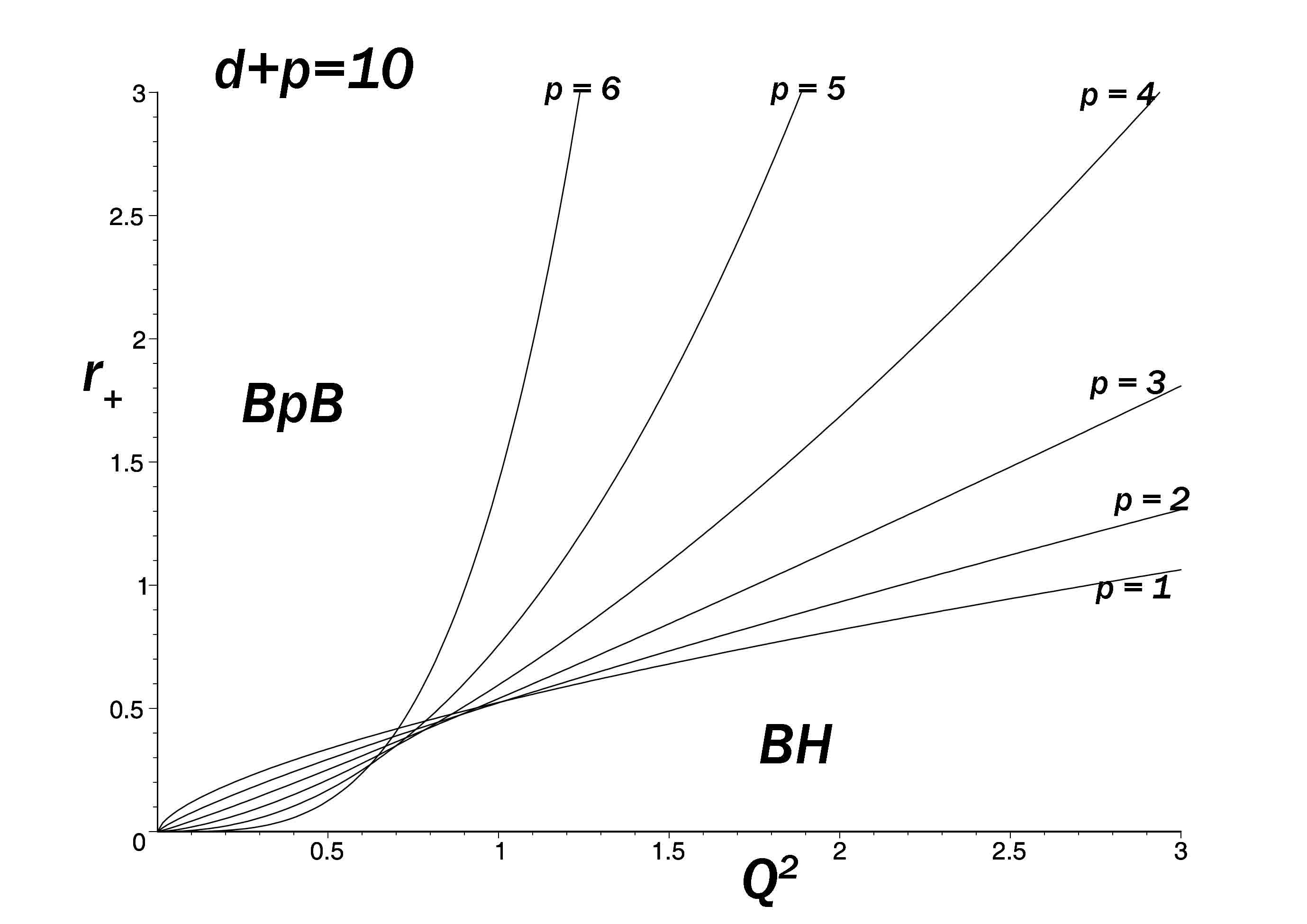
Figure 1: As a result of the entropy argument for the particular case $d+p=10$, we obtain this informative plot of BpB effective horizon radius $r_{+}$ versus common charge square $Q^{2}$. The horizon radius of BH, $r_{h}$, is connected to the horizon radius of BpB, $r_{+}$, through Eq. (77).

Let’s add that, the condition of equal temperature of the BpB and BH at the transition time yields a relation between the horizons of the two objects. This can be seen by equating (68) and (73) to find

$$r_{h}=\frac{\left(d+p-2\right)\left(d-3\right)}{2\left(d+p-3\right)\left(d+2p-2\right)}r_{+}^{\frac{d-2}{d+2p-2}}.$$ (81)

Therefore in Fig. 1, in the BH region, one has to compute the target black hole horizon radius by applying Eq. (77).

IV Conclusion

It is well-known that in asymptotically flat black holes stability lies at the heart of uniqueness which makes the Birkhoff theorem. By employing the thin-shell boundary condition we determine the mass available inside a shell of radius $r_{B}>r_{+}.$ In NAF-EYM theory we obtained for a particular class of solutions a critical boundary curve that separates BpB from BH bearing connected horizon radii but common charges $Q$. We argue that our stability treatment doesn’t depend on the particular solution but is more general. The NAF character manifests itself asymptotically as an AdS spacetime with a suitable effective cosmological constant. The critical curve arises from entropy comparison for the two types of black objects. It reflects the relative weight of dimensions $p$ and $d$ for each given case $d+p\geqslant 5$. In particular, we plotted $r_{+}$ versus $Q^{2}$ to represent the cases of $d+p=10$. The entropy comparison remains still a reliable test to check possible transitions from BpB to BH and vice versa. In this regard, we admit that our method applies only for charged black objects of special kind which doesn’t work for the neutral ones. We comment finally that in a recent study attention is drawn to the possibility of decay from a $5-$dimensional string into a set of $4-$dimensional naked singularities 29 . Transition into naked singularities has not been considered in the present work.

References

• (1) T. OrtΓ­n, Gravity and Strings (Cambridge University Press, Cambridge, 2006), p. 350.
• (2) T. Harmark, V. Niarchos and N. A. Obers, Class. Quatum Grav. 24, R1 (2007).
• (3) P. Bostock and S. F. Ross, Phys. Rev. DΒ 70, 064014 (2004).
• (4) T. Harmark and N. A. Obers, Nucl. Phys. B 684, 183 (2004).
• (5) R. Gregory and R. Laflamme, Phys. Rev. D 37, 305 (1988).
• (6) R. Emparan, H. Reall, Phys. Rev. Lett. 88 (2002) 101101.
• (7) R. Gregory and R. Laflamme, Phys. Rev. Lett. 70, 2837 (1993).
• (8) R. Gregory and R. Laflamme, Nucl. Phys. B 428, 399Β (1994).
• (9) U. Miyamoto, Phys. Lett. B 659, 380 (2008).
• (10) M. I. Park, Class. Quatum Grav. 22, 2607 (2005).
• (11) V. P. Frolov and A. A. Shoom. Phys. Rev. D 79, 104002 (2009).
• (12) B. Hartmann, Phys. Lett. B 602, 231 (2004).
• (13) Y. Brihaye and E. Radu, Phys. Lett. B 658, 164 (2008).
• (14) Y. Brihaye and B. Hartmann, Class. Quantum Grav. 22, 5145 (2005).
• (15) Y. Brihaye and T. Delsate, Phys. Rev. D 75, 044013 (2007).
• (16) J. D. Brown and J. W. York, Phys. Rev. D 47, 1407 (1993).
• (17) J. D. Brown, J. Creighton and R. B. Mann, Phys. Rev. D 50, 6394 (1994).
• (18) S. H. Mazharimousavi and M. Halilsoy, Phys. Rev. DΒ 76, 087501 (2007).
• (19) S. H. Mazharimousavi and M. Halilsoy, Phys. Lett. BΒ 659, 471 (2008).
• (20) S. H. Mazharimousavi and M. Halilsoy, Phys. Lett. BΒ 681, 190471 (2009).
• (21) S. H. Mazharimousavi, M. Halilsoy and Z. Amirabi, Gen Rel.Grav. 42, 261 (2010).
• (22) S. H. Mazharimousavi and M. Halilsoy, J. Cosmol. Astropart. Phys. 12, 005 (2008).
• (23) F. R. Tangherlini, Nuovo Cimento 27, 636 (1963)
• (24) G. Darmois 1927 MΓ©morial de Sciences MathΓ©matiques, Fascicule XXV Les equations de la gravitation einsteinienne ch V.
• (25) W. Israel, Nuovo Cimento B 44, 1 (1966).
• (26) W. Israel, Nuovo Cimento B 48, 463 (1966).
• (27) S. H. Mazharimousavi and M. Halilsoy, Eur. Phys. J. Plus 131, 138 (2016).
• (28) T. Muto, Phys. Lett. B 391, 310 (1997).
• (29) P. Figueras, M. Kunesch and S. Tunyasuvunakool, Phys. Rev. Lett. 116, 071102 (2016).