The Past and the Future in the Present

Abstract

We show how the shared information between the past and future—the excess entropy—derives from the components of directional information stored in the present—the predictive and retrodictive causal states. A detailed proof allows us to highlight a number of the subtle problems in estimation and analysis that impede accurate calculation of the excess entropy.

I Introduction

Predicting and modeling a system are distinct, but intimately related goals. Leveraging past observations, prediction attempts to make correct statements about what the future will bring, whereas modeling attempts to express the mechanisms behind the observations. In this view, building a model from observations is tantamount to decrypting a system’s hidden organization. The cryptographic view rests on the result that the apparent information shared between past and future—the excess entropy, which sets the bar for prediction—is only a function of the hidden stored information—the statistical complexity [1].

The excess entropy, and related mutual information quantities, though, are widely used diagnostics for complex systems, having been applied to detect the presence of organization in dynamical systems [2, 3, 4, 5], in spin systems  [6, 7], in neurobiological systems [8, 9], and even in human language [10, 11].

For the first time, Ref. [1] connected the observed sequence-based measure, the excess entropy, to a system’s internal structure and information processing. One consequence of the connection, and so our ability to differentiate between them, is that the excess entropy is an inadequate measure of a process’s organization. One must build models.

Our intention here is rather prosaic, however. We provide a focused and detailed proof of this relationship, which appears as Thm. 1 in Ref. [1] in a necessarily abbreviated form. A proof also appears in Ref. [12] employing a set of manipulations, developed but not laid out explicitly there, that require some facility with four-variable mutual informations and with subtle limiting properties of stochastic processes. The result is that directly expanding either of these concise proofs, without first deriving the rules, leads to apparent ambiguities.

The goal in the following is to present a step-by-step proof, motivating and explaining each step and attendant difficulties. The development also allows us to emphasize several new results that clarify the challenges in analytically calculating and empirically estimating these quantities. To get started, we give a minimal summary of the required background, assuming familiarity with Refs. [1] and [12], information theory [13], and information measures [14].

II Background

A process ${\Pr}(\overleftarrow{{X}},\overrightarrow{{X}})$ is a communication channel with a fixed input distribution ${\Pr}(\overleftarrow{{X}})$: It transmits information from the past $\overleftarrow{{X}}=\ldots{X}_{-3}{X}_{-2}{X}_{-1}$ to the future $\overrightarrow{{X}}={X}_{0}{X}_{1}{X}_{2}\ldots$ by storing it in the present. ${X}_{t}$ denotes the discrete random variable at time $t$ taking on values from an alphabet $\mathcal{A}$. A prediction of the process is specified by a distribution ${\Pr}(\overrightarrow{{X}}|{\overleftarrow{{x}}})$ of possible futures $\overrightarrow{{X}}$ given a particular past ${\overleftarrow{{x}}}$. At a minimum, a good predictor—call it $\widehat{{\cal R}}$—must capture all of a process’s excess entropy [15]—the information $I$ shared between past and future: ${\bf E}=I[\overleftarrow{{X}};\overrightarrow{{X}}]$. That is, for a good predictor: ${\bf E}=I[\widehat{{\cal R}};\overrightarrow{{X}}]$.

Building a model of a process is more demanding than developing a prediction scheme, though, as one wishes to express a process’s mechanisms and internal organization. To do this, computational mechanics introduced an equivalence relation ${\overleftarrow{{x}}}\sim{\overleftarrow{{x}}}^{\prime}$ that groups all histories which give rise to the same prediction. The result is a map $\epsilon:{\overleftarrow{\rm{\bf{X}}}}\to\bm{\mathcal{S}}$ from pasts to causal states defined by:

$$\epsilon({\overleftarrow{{x}}})=\{{\overleftarrow{{x}}}^{\prime}:{\Pr}(\overrightarrow{{X}}|{\overleftarrow{{x}}})={\Pr}(\overrightarrow{{X}}|{\overleftarrow{{x}}}^{\prime})\}~{}.$$ (1)

In other words, a process’s causal states are equivalence classes—$\bm{\mathcal{S}}={\Pr}(\overleftarrow{{X}},\overrightarrow{{X}})/\sim$—that partition the space ${\overleftarrow{\rm{\bf{X}}}}$ of pasts into sets which are predictively equivalent. The resulting model, consisting of the causal states and transitions, is called the process’s $\epsilon$-machine [16]. Out of all optimally predictive models $\bm{\widehat{{\cal R}}}$ resulting from a partition of the past, the $\epsilon$-machine captures the minimal amount of information that a process must store—the statistical complexity ${C_{\mu}}\equiv H[\mathcal{S}]$.

Said simply, ${\bf E}$ is the effective information transmission rate of the process, viewed as a channel, and ${C_{\mu}}$ is the sophistication of that channel. In general, the explicitly observed information ${\bf E}$ is only a lower bound on the information ${C_{\mu}}$ that a process stores [16].

The original development of $\epsilon$-machines concerned using the past to predict the future. One can, of course, use the future to retrodict the past by scanning the measurement variables in the reverse-time direction, as opposed to the default forward-time direction. With this in mind, the original map $\epsilon(\cdot)$ from pasts to causal states is denoted $\epsilon^{+}$ and it gave, what are called, the predictive causal states ${\bm{\mathcal{S}}}^{+}$. When scanning in the reverse direction, we have a new equivalence relation, $\overrightarrow{{x}}\sim^{-}\overrightarrow{{x}}^{\prime}$, that groups futures which are equivalent for the purpose of retrodicting the past: $\epsilon^{-}(\overrightarrow{{x}})=\{\overrightarrow{{x}}^{\prime}:{\Pr}(\overleftarrow{{X}}|\overrightarrow{{x}})={\Pr}(\overleftarrow{{X}}|\overrightarrow{{x}}^{\prime})\}$. It gives the retrodictive causal states ${\bm{\mathcal{S}}}^{-}={\Pr}(\overleftarrow{{X}},\overrightarrow{{X}})/\sim^{-}$.

In this bidirectional setting we have the forward-scan $\epsilon$-machine ${M}^{+}$ and its reverse-scan $\epsilon$-machine ${M}^{-}$. From them we can calculate corresponding entropy rates, $h_{\mu}^{+}$ and $h_{\mu}^{-}$, and statistical complexities, $C_{\mu}^{+}\equiv H[{\mathcal{S}}^{+}]$ and $C_{\mu}^{-}\equiv H[{\mathcal{S}}^{-}]$, respectively. Notably, while a stationary process is equally predictable in both directions of time—$h_{\mu}^{+}=h_{\mu}^{-}$—the amount of stored information differs in general: $C_{\mu}^{+}\neq C_{\mu}^{-}$ [1].

Recall that Thm. 1 of Ref. [1] showed that the shared information between the past $\overleftarrow{{X}}$ and future $\overrightarrow{{X}}$ is the mutual information between the predictive (${M}^{+}$’s) and retrodictive (${M}^{-}$’s) causal states:

$${\bf E}=I[{\mathcal{S}}^{+};{\mathcal{S}}^{-}]~{}.$$ (2)

This led to the view that the process’s channel utilization $I[\overleftarrow{{X}};\overrightarrow{{X}}]$ is the same as that in the channel between a process’s forward and reverse causal states.

To understand how the states of the forward and reverse $\epsilon$-machines capture information from the past and the future—and to avoid the ambiguities alluded to earlier—we must analyze a four-variable mutual information: $I[\overleftarrow{{X}};\overrightarrow{{X}};{\mathcal{S}}^{+};{\mathcal{S}}^{-}]$. A large number of expansions of this quantity are possible. A systematic development follows from Ref. [14] which showed that Shannon entropy $H[\cdot]$ and mutual information $I[\cdot\,;\cdot]$ form a signed measure over the space of events.

III Two Issues

The theorem’s proof can be expressed in a very compact way using several (implied) rules:

$${\bf E} =I[\overleftarrow{{X}};\overrightarrow{{X}}]$$ (3)

$$=I[\epsilon^{+}(\overleftarrow{{X}});\epsilon^{-}(\overrightarrow{{X}})]$$ (4)

$$=I[{\mathcal{S}}^{+};{\mathcal{S}}^{-}]~{}.$$ (5)

While this proof conveys the essential meaning and, being short, is easily intuited, there are two issues with it. The concern is that, if the concise proof is misinterpreted or the rules not heeded, confusion arises. Refs. [1] and [12] develop the appropriate rules, but do not lay them out explicitly.

The first issue is that naive expansion of the past-future mutual informations leads to ambiguously interpretable quantities. The second issue is that implicitly there are Shannon entropies—e.g., $H[\overleftarrow{{X}}]$ and $H[\overrightarrow{{X}}]$—over semi-infinite chains of random variables and these entropies diverge in the general case. Here, via an exegesis of the concise proof, we show how to address these two problems and, along the way, explicate several of the required rules. We diagnose the first issue and then provide a new step-by-step proof, ignoring the second issue of divergent quantities. We end by showing how to work systematically with divergent entropies.

IV Comparable Objects and Sufficiency

The first problem comes from inappropriate application of the $\epsilon(\cdot)$ functions. The result is the inadvertent introduction of incomparable quantities. Namely,

$${\Pr}(\overrightarrow{{X}}|\overleftarrow{{X}}) ={\Pr}(\overrightarrow{{X}}|\epsilon^{+}(\overleftarrow{{X}}))$$

$$={\Pr}(\overrightarrow{{X}}|{\mathcal{S}}^{+})$$ (6)

is a proper use of the predictive causal equivalence relation—the probabilities at each stage refer to the same object, the future $\overrightarrow{{X}}$. We say that the predictive causal states are sufficient statistics for the future.

The following use (in the first equality) is incorrect, however:

$${\Pr}(\overleftarrow{{X}}) ={\Pr}(\epsilon^{+}(\overleftarrow{{X}}))$$

$$={\Pr}({\mathcal{S}}^{+})~{},$$

even though it appears as a straightforward (and analogous) application of the causal equivalence relation. The problem occurs since the first equality incorrectly conflates probability of two different objects—a future and a causal state; an element and a set. A handy mnemonic for the appearance of this error is to interpret the expression literally: typically, a causal state has positive probability, but an infinite future has zero probability. Clearly, a wrong statement.

There are restrictions on when the causal equivalence relation can be applied. In particular, in the shorthand proof of Thm. 1 above, there are ambiguous expansions of the mutual information that lead one to such errors. These must be avoided.

Specifically, the step (Eq. (4)) involving the simultaneous application of the forward and reverse causal equivalence relations must be done with care. Here, we show how to do this. But, first, let’s explore the problem a bit more. Starting from Eq. (3), we go one step at a time:

$$I[\overleftarrow{{X}};\overrightarrow{{X}}] =I[\epsilon^{+}(\overleftarrow{{X}});\overrightarrow{{X}}]$$

$$=I[{\mathcal{S}}^{+};\overrightarrow{{X}}]~{}.$$ (7)

The result is correct, largely because one has in mind the more detailed series of steps using the mutual information’s component entropies. That is, let’s redo the preceding:

$$I[\overleftarrow{{X}};\overrightarrow{{X}}] =H[\overrightarrow{{X}}]-H[\overrightarrow{{X}}|\overleftarrow{{X}}]$$

$$=H[\overrightarrow{{X}}]-H[\overrightarrow{{X}}|\epsilon^{+}(\overleftarrow{{X}})]$$ (8)

$$=H[\overrightarrow{{X}}]-H[\overrightarrow{{X}}|{\mathcal{S}}^{+}]$$

$$=I[{\mathcal{S}}^{+};\overrightarrow{{X}}]~{}.$$ (9)

Notice that the application of $\epsilon^{+}(\cdot)$ occurs only in conditioning. Also, for the sake of argument, we temporarily ignore the appearance of the potentially infinite quantity $H[\overrightarrow{{X}}]$.

To emphasize the point, it is incorrect to continue the same strategy, however. That is, picking up from Eq. (9) the following is ambiguous:

$$I[\overleftarrow{{X}};\overrightarrow{{X}}] =I[{\mathcal{S}}^{+};\overrightarrow{{X}}]$$

$$=I[{\mathcal{S}}^{+};\epsilon^{-}(\overrightarrow{{X}})]$$

$$=I[{\mathcal{S}}^{+};{\mathcal{S}}^{-}]$$

even though the final line is the goal and, ultimately, is correct. Why? To see this, we again expand out the intermediary steps implied:

$$I[{\mathcal{S}}^{+};\overrightarrow{{X}}] =H[\overrightarrow{{X}}]-H[\overrightarrow{{X}}|{\mathcal{S}}^{+}]$$ (10)

$$=H[\epsilon^{-}(\overrightarrow{{X}})]-H[\epsilon^{-}(\overrightarrow{{X}})|{\mathcal{S}}^{+}]$$ (11)

$$=H[{\mathcal{S}}^{-}]-H[{\mathcal{S}}^{-}|{\mathcal{S}}^{+}]$$

$$=I[{\mathcal{S}}^{-};{\mathcal{S}}^{+}]~{}.$$

That second step (Eq. (11)), by violating the rule of matching objects types, is wrong. And so, the ensuing steps do not follow, even if the desired result is obtained.

The conclusion is that the second use of the causal equivalence relation, seemingly forced in the original short proof of Thm. 1, is not valid. The solution is to find a different proof strategy that does not lead to this cul de sac.

There is an alternative expansion to Eq. (10) that appears to avoid the problem:

$$I[{\mathcal{S}}^{+};\overrightarrow{{X}}] =H[{\mathcal{S}}^{+}]-H[{\mathcal{S}}^{+}|\overrightarrow{{X}}]$$

$$=H[{\mathcal{S}}^{+}]-H[{\mathcal{S}}^{+}|\epsilon^{-}(\overrightarrow{{X}})]$$ (12)

$$=H[{\mathcal{S}}^{+}]-H[{\mathcal{S}}^{+}|{\mathcal{S}}^{-}]$$

$$=I[{\mathcal{S}}^{-};{\mathcal{S}}^{+}]~{}.$$

This seems fine, since no overtly infinite quantities appear and $\epsilon^{-}(\cdot)$ is used only in conditioning.

The step to Eq. (12) is still problematic, though. The concern is that, on the one hand, the retrodictive causal states are sufficient for the pasts, as indicated in Eq. (6). On the other hand, it does not immediately follow that they are sufficient for predictive causal states, as required by Eq. (12).

In short, these problems result from ignoring that the goal involves a higher-dimensional, multivariate problem. We need a strategy that avoids the ambiguities and gives a reliable procedure. This is found in using the four-variable mutual informations introduced in Refs. [1] and [12]. This is the strategy we now lay out and it also serves to illustrate the rules required for the more concise proof strategy.

V Detailed Proof

In addition to the rule of not introducing incomparable objects, we need several basic results. First, the causal equivalence relations lead to the informational identities:

$$H[{\mathcal{S}}^{+}|\overleftarrow{{X}}] =0~{},$$

$$H[{\mathcal{S}}^{-}|\overrightarrow{{X}}] =0~{}.$$

That is, these state uncertainties vanish, since $\epsilon^{+}(\cdot)$ and $\epsilon^{-}(\cdot)$ are functions, respectively, of the past and future.

Second, causal states have the Markovian property that they render the past and future statistically independent. They causally shield the future from the past:

$$I[\overleftarrow{{X}};\overrightarrow{{X}}|{\mathcal{S}}^{+}] =0~{},$$

$$I[\overleftarrow{{X}};\overrightarrow{{X}}|{\mathcal{S}}^{-}] =0~{}.$$

In this way, one sees how the causal states are the structural decomposition of a process into conditionally independent modules. Moreover, they are defined to be optimally predictive in the sense that knowing which causal state a process is in is just as good as having the entire past in hand: ${\Pr}(\overrightarrow{{X}}|{\mathcal{S}}^{+})={\Pr}(\overrightarrow{{X}}|\overleftarrow{{X}})$ or, equivalently, ${\bf E}=I[{\mathcal{S}}^{+};\overrightarrow{{X}}]$.

Now, we consider several additional identities that follow more or less straightforwardly from the $\epsilon$-machine’s defining properties.

Lemma 1.

$I[{\mathcal{S}}^{+};{\mathcal{S}}^{-}|\overleftarrow{{X}}]=0$ and $I[{\mathcal{S}}^{+};{\mathcal{S}}^{-}|\overrightarrow{{X}}]=0$.

Proof.

These vanish since the past (future) determines the predictive (retrodictive) causal state. ∎

Lemma 2.

$I[\overleftarrow{{X}};\overrightarrow{{X}};{\mathcal{S}}^{-}|{\mathcal{S}}^{+}]=0$.

Proof.

$$I[\overleftarrow{{X}};\overrightarrow{{X}};{\mathcal{S}}^{+}|{\mathcal{S}}^{-}] =I[\overleftarrow{{X}};\overrightarrow{{X}}|{\mathcal{S}}^{-}]-I[\overleftarrow{{X}};\overrightarrow{{X}}|{\mathcal{S}}^{+},{\mathcal{S}}^{-}]$$

$$=0-0~{}.$$

The terms vanish by causal shielding. ∎

Lemma 3.

$I[{\mathcal{S}}^{+};{\mathcal{S}}^{-};\overrightarrow{{X}}|\overleftarrow{{X}}]=0$.

Proof.

$$I[{\mathcal{S}}^{+};{\mathcal{S}}^{-};\overrightarrow{{X}}|\overleftarrow{{X}}] =I[{\mathcal{S}}^{+};{\mathcal{S}}^{-}|\overleftarrow{{X}}]$$

$$~{}~{}~{}-I[{\mathcal{S}}^{+};{\mathcal{S}}^{-}|\overleftarrow{{X}},\overrightarrow{{X}}]~{}.$$

The first term vanishes by Lemma 1. Expanding the second term we see that:

$$I[{\mathcal{S}}^{+};{\mathcal{S}}^{-}|\overleftarrow{{X}},\overrightarrow{{X}}] =H[{\mathcal{S}}^{+}|\overleftarrow{{X}},\overrightarrow{{X}}]$$

$$~{}~{}~{}~{}-H[{\mathcal{S}}^{+}|\overleftarrow{{X}},\overrightarrow{{X}},{\mathcal{S}}^{-}]~{}.$$

Both terms here vanish since the past determines the predictive causal state. ∎

Now, we are ready for the proof. First, recall the theorem’s statement.

Theorem 1.

Excess entropy is the mutual information between the predictive and retrodictive causal states:

$${\bf E}=I[{\mathcal{S}}^{+};{\mathcal{S}}^{-}]~{}.$$ (13)

Proof.

This follows via a parallel reduction of the four-variable mutual information $I[\overleftarrow{{X}};\overrightarrow{{X}};{\mathcal{S}}^{+};{\mathcal{S}}^{-}]$ into $I[\overleftarrow{{X}};\overrightarrow{{X}}]$ and $I[{\mathcal{S}}^{+};{\mathcal{S}}^{-}]$. The first reduction is:

$$I[\overleftarrow{{X}};\overrightarrow{{X}};{\mathcal{S}}^{+};{\mathcal{S}}^{-}] =I[\overleftarrow{{X}};\overrightarrow{{X}};{\mathcal{S}}^{+}]-I[\overleftarrow{{X}};\overrightarrow{{X}};{\mathcal{S}}^{+}|{\mathcal{S}}^{-}]$$

$$=I[\overleftarrow{{X}};\overrightarrow{{X}};{\mathcal{S}}^{+}]$$

$$=I[\overleftarrow{{X}};\overrightarrow{{X}}]-I[\overleftarrow{{X}};\overrightarrow{{X}}|{\mathcal{S}}^{+}]$$

$$=I[\overleftarrow{{X}};\overrightarrow{{X}}]$$

$$={\bf E}~{}.$$

The second line follows from Lemma 2 and the fourth from causal shielding.

The second reduction is, then:

$$I[\overleftarrow{{X}};\overrightarrow{{X}};{\mathcal{S}}^{+};{\mathcal{S}}^{-}] =I[{\mathcal{S}}^{+};{\mathcal{S}}^{-};\overrightarrow{{X}}]-I[{\mathcal{S}}^{+};{\mathcal{S}}^{-};\overrightarrow{{X}}|\overleftarrow{{X}}]$$

$$=I[{\mathcal{S}}^{+};{\mathcal{S}}^{-};\overrightarrow{{X}}]$$

$$=I[{\mathcal{S}}^{+};{\mathcal{S}}^{-}]-I[{\mathcal{S}}^{+};{\mathcal{S}}^{-}|\overrightarrow{{X}}]$$

$$=I[{\mathcal{S}}^{+};{\mathcal{S}}^{-}]~{}.$$

The second line follows from Lemma 3 and the fourth from Lemma 1. ∎

Remark.

Note that the steps here do not force one into inadvertently using the causal equivalence relation to introduce incomparable objects.

VI Finite Pasts and Futures

This is all well and good, but there is a nagging concern in all of the above. As noted at the beginning, we are improperly using entropies of semi-infinite chains of random variables. These entropies typically are infinite and so many of the steps are literally not correct. Fortunately, as we will show, this concern is so directly addressed that there is rarely an inhibition in the above uses. The shortcuts that allow their use are extremely handy and allow much progress and insight, if deployed with care. Ultimately, of course, one must still go through proofs using proper objects and manipulations and verifying limits. We now show how to address this issue, highlighting a number of technicalities that distinguish between important process classes.

The strategy is straightforward, if somewhat tedious and obfuscating: Define pasts, futures, and causal states over finite-length sequences.

Definition.

Given a process $\Pr(\overleftrightarrow{{X}})$, its finite predictive causal states ${\mathcal{S}}^{+}_{KL}$ are defined by:

$$\epsilon^{+}_{KL}(\overleftarrow{{x}}^{K})\equiv\left\{\overleftarrow{{x}}^{\prime{K}}:{\Pr}(\overrightarrow{{X}}^{L}|\overleftarrow{{x}}^{K})={\Pr}(\overrightarrow{{X}}^{L}|\overleftarrow{{x}}^{\prime{K}})\right\}~{}.$$

Definition.

Given a process $\Pr(\overleftrightarrow{{X}})$, its finite retrodictive causal states ${\mathcal{S}}^{-}_{KL}$ are defined by:

$$\epsilon^{-}_{KL}(\overrightarrow{{x}}^{L})\equiv\left\{\overrightarrow{{x}}^{\prime{L}}:{\Pr}(\overleftarrow{{X}}^{K}|\overrightarrow{{x}}^{L})={\Pr}(\overleftarrow{{X}}^{K}|\overrightarrow{{x}}^{L})\right\}~{}.$$

That is, we now partition finite pasts (futures) of length $K$ ($L$) with probabilistically distinct distributions over finite futures (pasts). We end up with two sets, ${\bm{\mathcal{S}}}^{+}_{KL}$ and ${\bm{\mathcal{S}}}^{-}_{KL}$, which describe the finite-length predictive and retrodictive causal states for each value of $K$ and $L$.

Remark.

The subscripts on ${\mathcal{S}}^{+}_{KL}$ and ${\mathcal{S}}^{-}_{KL}$ should not be interpreted as time indices, as they are more commonly used in the literature.

Remark.

A central issue here is that, in general, for the causal states ${\mathcal{S}}^{+}$ defined by Eq. (1):

$${\mathcal{S}}^{+}\neq\lim_{K,L\rightarrow\infty}{\mathcal{S}}^{+}_{KL}~{}.$$ (14)

The analogous situation is true for ${\mathcal{S}}^{-}$. Why? For some processes, it can happen that $|{\bm{\mathcal{S}}}^{+}_{KL}|\to\infty$ even though $|{\bm{\mathcal{S}}}^{+}|<\infty$. The result is that the causal states ${\mathcal{S}}^{+}$ are not reached in the above limiting procedure. However, their information content can be the same. And so, in the following, we must take care in establishing results regarding the large-$K$ and -$L$ limits.

A first example of this is to explain why the applications of $\epsilon(\cdot)$ in Eqs. (7) and (8) are plausible. We establish the finite-length version of those steps.

Proposition 1.

$H[\overrightarrow{{X}}^{L}|\overleftarrow{{X}}^{K}]=H[\overrightarrow{{X}}^{L}|{\mathcal{S}}^{+}_{KL}]$.

Proof.

We calculate directly:

$$H[ \overrightarrow{{X}}^{L}|\overleftarrow{{X}}^{K}]$$

$$=\sum_{\mathchoice{\hbox to0.0pt{\hss$\displaystyle{w\in\mathcal{A}^{K}}$\hss}}{\hbox to0.0pt{\hss$\textstyle{w\in\mathcal{A}^{K}}$\hss}}{\hbox to0.0pt{\hss$\scriptstyle{w\in\mathcal{A}^{K}}$\hss}}{\hbox to0.0pt{\hss$\scriptscriptstyle{w\in\mathcal{A}^{K}}$\hss}}}{\Pr}(w)H[\overrightarrow{{X}}^{L}|\overleftarrow{{X}}^{K}=w]$$

$$=\sum_{\mathchoice{\hbox to0.0pt{\hss$\displaystyle{w\in\mathcal{A}^{K}}$\hss}}{\hbox to0.0pt{\hss$\textstyle{w\in\mathcal{A}^{K}}$\hss}}{\hbox to0.0pt{\hss$\scriptstyle{w\in\mathcal{A}^{K}}$\hss}}{\hbox to0.0pt{\hss$\scriptscriptstyle{w\in\mathcal{A}^{K}}$\hss}}}{\Pr}(w)H[\overrightarrow{{X}}^{L}|{\mathcal{S}}^{+}_{KL}=\epsilon^{+}_{KL}(w)]$$

$$=\sum_{\mathchoice{\hbox to0.0pt{\hss$\displaystyle{w\in\mathcal{A}^{K}}$\hss}}{\hbox to0.0pt{\hss$\textstyle{w\in\mathcal{A}^{K}}$\hss}}{\hbox to0.0pt{\hss$\scriptstyle{w\in\mathcal{A}^{K}}$\hss}}{\hbox to0.0pt{\hss$\scriptscriptstyle{w\in\mathcal{A}^{K}}$\hss}}}{\Pr}(w)H[\overrightarrow{{X}}^{L}|{\mathcal{S}}^{+}_{KL}=\epsilon^{+}_{KL}(w)]\sum_{\mathchoice{\hbox to0.0pt{\hss$\displaystyle{\sigma\in{\bm{\mathcal{S}}}^{+}_{KL}}$\hss}}{\hbox to0.0pt{\hss$\textstyle{\sigma\in{\bm{\mathcal{S}}}^{+}_{KL}}$\hss}}{\hbox to0.0pt{\hss$\scriptstyle{\sigma\in{\bm{\mathcal{S}}}^{+}_{KL}}$\hss}}{\hbox to0.0pt{\hss$\scriptscriptstyle{\sigma\in{\bm{\mathcal{S}}}^{+}_{KL}}$\hss}}}\delta_{\sigma,\epsilon^{+}_{KL}(w)}$$

$$=\sum_{\mathchoice{\hbox to0.0pt{\hss$\displaystyle{\sigma\in{\bm{\mathcal{S}}}^{+}_{KL}}$\hss}}{\hbox to0.0pt{\hss$\textstyle{\sigma\in{\bm{\mathcal{S}}}^{+}_{KL}}$\hss}}{\hbox to0.0pt{\hss$\scriptstyle{\sigma\in{\bm{\mathcal{S}}}^{+}_{KL}}$\hss}}{\hbox to0.0pt{\hss$\scriptscriptstyle{\sigma\in{\bm{\mathcal{S}}}^{+}_{KL}}$\hss}}}H[\overrightarrow{{X}}^{L}|{\mathcal{S}}^{+}_{KL}=\sigma]\sum_{\mathchoice{\hbox to0.0pt{\hss$\displaystyle{w\in\mathcal{A}^{K}}$\hss}}{\hbox to0.0pt{\hss$\textstyle{w\in\mathcal{A}^{K}}$\hss}}{\hbox to0.0pt{\hss$\scriptstyle{w\in\mathcal{A}^{K}}$\hss}}{\hbox to0.0pt{\hss$\scriptscriptstyle{w\in\mathcal{A}^{K}}$\hss}}}{\Pr}(w)\delta_{\sigma,\epsilon^{+}_{KL}(w)}$$

$$=\sum_{\mathchoice{\hbox to0.0pt{\hss$\displaystyle{\sigma\in{\bm{\mathcal{S}}}^{+}_{KL}}$\hss}}{\hbox to0.0pt{\hss$\textstyle{\sigma\in{\bm{\mathcal{S}}}^{+}_{KL}}$\hss}}{\hbox to0.0pt{\hss$\scriptstyle{\sigma\in{\bm{\mathcal{S}}}^{+}_{KL}}$\hss}}{\hbox to0.0pt{\hss$\scriptscriptstyle{\sigma\in{\bm{\mathcal{S}}}^{+}_{KL}}$\hss}}}H[\overrightarrow{{X}}^{L}|{\mathcal{S}}^{+}_{KL}=\sigma]{\Pr}(\sigma)$$

$$=H[\overrightarrow{{X}}^{L}|{\mathcal{S}}^{+}_{KL}]~{}.\hskip 108.405pt\qed$$

And so, for all $L$, we have:

$$H[\overrightarrow{{X}}^{L}|{\mathcal{S}}^{+}_{\infty L}] \equiv\lim_{K\rightarrow\infty}H[\overrightarrow{{X}}^{L}|{\mathcal{S}}^{+}_{KL}]$$

$$=\lim_{K\rightarrow\infty}H[\overrightarrow{{X}}^{L}|\overleftarrow{{X}}^{K}]$$

$$=H[\overrightarrow{{X}}^{L}|\overleftarrow{{X}}]~{}.$$

The last step requires a measure-theoretic justification. This is given using the method of Ref. [17, Appendix].

Corollary 1.

$I[\overleftarrow{{X}}^{K};\overrightarrow{{X}}^{L}]=I[{\mathcal{S}}^{+}_{KL};\overrightarrow{{X}}^{L}]$.

Proof.

Following a finite-lengths version of Eq. (7), we apply Prop. 1.

By similar reasoning in the proposition and corollary we have the time-reversed analogs:

$$H[\overleftarrow{{X}}^{K}|\overrightarrow{{X}}^{L}] =H[\overleftarrow{{X}}^{K}|{\mathcal{S}}^{-}_{KL}]~{},$$

$$I[\overleftarrow{{X}}^{K};\overrightarrow{{X}}^{L}] =I[\overleftarrow{{X}}^{K};{\mathcal{S}}^{-}_{KL}]~{}.$$

Definition.

The finite-length excess entropy is:

$${\bf E}(K,L)\equiv I[\overleftarrow{{X}}^{K};\overrightarrow{{X}}^{L}]~{}.$$

Lemma 4.

${\bf E}=\lim_{K,L\to\infty}{\bf E}(K,L)$.

Proof.

It is known that $I[\overleftarrow{{X}}^{L};\overrightarrow{{X}}^{L}]$ converges to ${\bf E}$ [15, 18]. Thus, it follows straightforwardly that $I[\overleftarrow{{X}}^{K};\overrightarrow{{X}}^{L}]$ also converges to ${\bf E}$, so long as $K$ and $L$ simultaneously diverge to infinity. ∎

We are now, finally, ready to focus in more directly on the original goal.

Proposition 2.

${\bf E}(K,L)=I[{\mathcal{S}}^{+}_{KL};{\mathcal{S}}^{-}_{KL}]$.

Proof.

The proof relies on finite-length analogs to Lemmas 1, 2, and 3 and then proceeds similarly to Thm. 1. Specifically,

$$I[\overleftarrow{{X}}^{K};{\mathcal{S}}^{+}_{KL};{\mathcal{S}}^{-}_{KL};\overrightarrow{{X}}^{L}] =I[\overleftarrow{{X}}^{K};\overrightarrow{{X}}^{L}]$$

follows from the first reduction in the proof of Thm. 1 and:

$$I[\overleftarrow{{X}}^{K};{\mathcal{S}}^{+}_{KL};{\mathcal{S}}^{-}_{KL};\overrightarrow{{X}}^{L}] =I[{\mathcal{S}}^{+}_{KL};{\mathcal{S}}^{-}_{KL}]$$

follows from the second reduction there. All that is changed in the reductions is the substitution of finite-length quantities. Otherwise, the information-theoretic identities hold as given there. ∎

Theorem 2.

The excess entropy is:

$${\bf E}=\lim_{K,L\to\infty}I[{\mathcal{S}}^{+}_{KL};{\mathcal{S}}^{-}_{KL}]~{}.$$

Proof.

By Lemma 4, we relate ${\bf E}$ to the sequence of mutual informations between the finite past and finite future. By Prop. 2, this limit is also equal to the limit of mutual informations between the finite predictive and finite retrodictive causal states. ∎

Remark.

As with Lemma 4, the limits in $K$ and $L$ must be done simultaneously.

At this point, we have gone as far as possible, it seems, in relating the finite-length excess entropy and forward-reverse causal-state mutual informations. From here on, different kinds of process have different limiting behaviors. We discuss one such class and so establish the original claim.

Recall the class of processes that can be represented by exactly synchronizing $\epsilon$-machines. Roughly speaking, such a process has an $\epsilon$-machine to which an observer comes to know its internal state from a finite number of measurements. (For background see Ref. [18].) This is the class of processes we focus on in the following.

Lemma 5.

If ${M}^{+}$ and ${M}^{-}$ are both exactly synchronizing and each has a finite number of (recurrent) causal states, then:

$$I[{\mathcal{S}}^{+};{\mathcal{S}}^{-}]=\lim_{K,L\rightarrow\infty}I[{\mathcal{S}}^{+}_{KL};{\mathcal{S}}^{-}_{KL}]~{}.$$ (15)

Proof.

Finitary processes that are exactly synchronizable have at least one finite-length synchronizing word. And this sync word occurs in almost every sufficiently long sequence. Thus, as $K$ and $L$ simultaneously tend to infinity, one eventually constructs a partition that includes a synchronizing word. From there on, increasing $K$ and $L$ eventually discovers all infinite-length causal states, which are finite in number by assumption. The result is that probability accumulates in the subset of finite-length causal states which correspond to the causal states which are reachable, infinitely-preceded, and recurrent [19]. Thus, the limit of the finite-length causal states differs from the infinite-length causal states only on a set of measure zero. Finally, also by assumption, this holds for both the forward and reverse $\epsilon$-machines. And so, the information content in the finite-length causal states limits on the information content of the causal states which, by Eq. (1), are defined in terms of semi-infinite pasts and futures. ∎

Theorem 3.

If ${M}^{+}$ and ${M}^{-}$ are both exactly synchronizing and each has a finite number of (recurrent) causal states, then:

$${\bf E}=I[{\mathcal{S}}^{+};{\mathcal{S}}^{-}]~{}.$$

Proof.

Directly from Thm. 2 and Lemma 5.

VII Conclusion

In the preceding, we examined an evocative and, in its simplicity, innocent-looking identity: ${\bf E}=I[{\mathcal{S}}^{+};{\mathcal{S}}^{-}]$. It tells us that the excess entropy is equal to the mutual information between the predictive and retrodictive causal states. It begins to reveal its subtleties when one realizes that excess entropy is defined solely in terms of the observed process $\Pr(\overleftarrow{{X}};\overrightarrow{{X}})$ and makes no explicit reference to the process’s internal organization. Additionally, $\overleftarrow{{X}}$ and $\overrightarrow{{X}}$ are continuous random variables, when ${\mathcal{S}}^{+}$ and ${\mathcal{S}}^{-}$ need not be.

In explicating their relationships, finite-length counterparts to the predictive and retrodictive causal states were introduced, and the limit was taken as the finite-lengths tended to infinity. A priori, there is no reason to expect that the finite-length causal states will limit on the causal states, since the latter are defined over infinite histories and futures. In fact, there are finitary processes for which the number of finite-length causal states diverges, even when the number of (asymptotic, recurrent) causal states is finite.

However, when considering exactly synchronizing $\epsilon$-machines, there exists a subset of the finite-length causal states at each $K$ and $L$ that does limit on the causal states. When such $\epsilon$-machines have a finite number of causal states, it is possible to identify this subset. This fact was used to prove Thm. 5.

When this subset of the finite-length causal states cannot be identified or when it does not exist, it is still expected that the limit of mutual informations between the finite-length causal states will equal the mutual information between the predictive and retrodictive causal states. However, the proof for this requires more sophistication and the technique for calculating ${\bf E}$, outlined in Ref. [12], needs refining. The set of $\epsilon$-machines that are not exactly synchronizing are among those that would benefit from such analysis.

The information diagram of Figure 1 closes our development by summarizing the more detailed finite-history and -future framework introduced here. The various lemmas, showing that this or that mutual information vanished, translate into information-measure atoms having zero area. The overall diagram is quite similar to that introduced in Ref. [1], which serves to emphasize the point made earlier that working with infinite sequences preserves many of the central relationships in a process’s information measure. It also does not suffer from the criticism, as did the previous one, of representing infinite atoms as finite.

The information diagram graphically demonstrates that, as done in the detailed proof given for Thm. 3, one should avoid using potentially infinite quantities, such as $H[\overleftarrow{{X}}]$ and $H[\overrightarrow{{X}}]$, whenever possible, in favor of alternative finite atoms, which are various mutual informations and conditional mutual informations. Moreover, when infinite atoms cannot be avoided, then the finite-length quantities must be used and their limits carefully taken, as we showed.

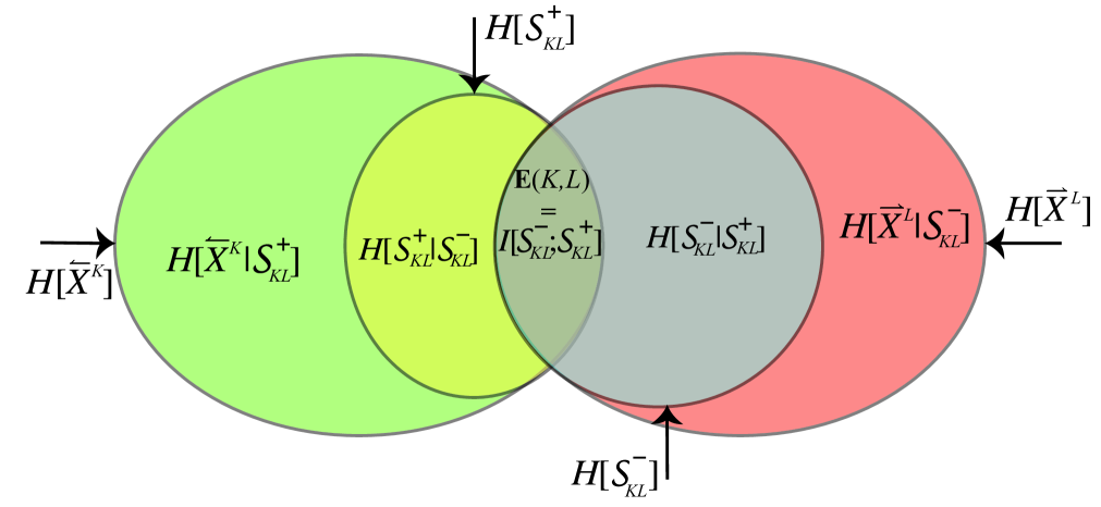
Figure 1: $\epsilon$-Machine information diagram over finite length-$K$ past and length-$L$ future sequences for a stationary stochastic process.

References

- [1] J. P. Crutchfield, C. J. Ellison, and J. R. Mahoney. Time’s barbed arrow: Irreversibility, crypticity, and stored information. Phys. Rev. Lett., 103(9):094101, 2009.
- [2] A. Fraser and H. L. Swinney. Independent coordinates for strange attractors from mutual information. Phys. Rev. A, 33:1134–1140, 1986.
- [3] M. Casdagli and S. Eubank, editors. Nonlinear Modeling, SFI Studies in the Sciences of Complexity, Reading, Massachusetts, 1992. Addison-Wesley.
- [4] J. C. Sprott. Chaos and Time-Series Analysis. Oxford University Press, Oxford, UK, second edition, 2003.
- [5] H. Kantz and T. Schreiber. Nonlinear Time Series Analysis. Cambridge University Press, Cambridge, UK, second edition, 2006.
- [6] J. P. Crutchfield and D. P. Feldman. Statistical complexity of simple one-dimensional spin systems. Phys. Rev. E, 55(2):R1239–R1243, 1997.
- [7] I. Erb and N. Ay. Multi-information in the thermodynamic limit. J. Stat. Phys., 115:949–967, 2004.
- [8] G. Tononi, O. Sporns, and G. M. Edelman. A measure for brain complexity: Relating functional segregation and integration in the nervous system. Proc. Nat. Acad. Sci. USA, 91:5033–5037, 1994.
- [9] W. Bialek, I. Nemenman, and N. Tishby. Predictability, complexity, and learning. Neural Computation, 13:2409–2463, 2001.
- [10] W. Ebeling and T. Poschel. Entropy and long-range correlations in literary english. Europhys. Lett., 26:241–246, 1994.
- [11] L. Debowski. On the vocabulary of grammar-based codes and the logical consistency of texts. 2008. submitted; arXiv.org:0810.3125 [cs.IT].
- [12] C. J. Ellison, J. R. Mahoney, and J. P. Crutchfield. Prediction, retrodiction, and the amount of information stored in the present. J. Stat. Phys., 136(6):1005–1034, 2009.
- [13] T. M. Cover and J. A. Thomas. Elements of Information Theory. Wiley-Interscience, New York, second edition, 2006.
- [14] R. Yeung. A new outlook on Shannon’s information measures. IEEE Trans. Info. Th., 37(3):466–474, 1991.
- [15] J. P. Crutchfield and D. P. Feldman. Regularities unseen, randomness observed: Levels of entropy convergence. CHAOS, 13(1):25–54, 2003.
- [16] J. P. Crutchfield and K. Young. Inferring statistical complexity. Phys. Rev. Let., 63:105–108, 1989; J. P. Crutchfield, Physica D 75 11–54, 1994; J. P. Crutchfield and C. R. Shalizi, Phys. Rev. E 59(1) 275–283, 1999.
- [17] N. Travers and J. P. Crutchfield. Equivalence of history and generator epsilon-machines. 2010. SFI Working Paper 10-12-XXX; arxiv.org:1012.XXXX [XXXX].
- [18] N. Travers and J. P. Crutchfield. Asymptotic synchronization for finite-state sources. submitted, 2010. arxiv:1011.1581 [nlin.CD].
- [19] D. R. Upper. Theory and Algorithms for Hidden Markov Models and Generalized Hidden Markov Models. PhD thesis, University of California, Berkeley, 1997. Published by University Microfilms Intl, Ann Arbor, Michigan.