Bulk viscosity in the nonlinear and anharmonic regime of strange quark matter

Abstract

The bulk viscosity of cold, dense three-flavor quark matter is studied as a function of temperature and the amplitude of density oscillations. The study is also extended to the case of two different types of anharmonic oscillations of density. We point several qualitative effects due to the anharmonicity, although quantitatively they appear to be relatively small. We also find that, in most regions of the parameter space, with the exception of the case of a very large amplitude of density oscillations (i.e. $10\%$ and above), nonlinear effects and anharmonicity have a small effect on the interplay of the nonleptonic and semileptonic processes in the bulk viscosity.

1 Introduction

Cold, dense quark matter is one of possible states of baryonic matter formed at very high densities. While there is little doubt that such quark matter can be formed in principle, the value of the critical density needed remains unknown. This is one of the reasons why it is not settled whether such form of matter can exist inside neutron stars. Indeed, the interior region of neutron stars is the most likely place to find dense quark matter. The corresponding densities reach up to about 10 times the nuclear saturation density, while the temperatures remain moderately low, of the order of $1~{}\mbox{MeV}$ or less.

A recent report on a precision measurement of the mass of the binary millisecond pulsar J1614-2230 [1] seems to strongly constraint the possibility of stellar dense quark matter [2]. Nevertheless, it is hard to rule out quark matter solely based on the measurement of such a global property of a star such as its mass.. More informative probes of the state of matter at the highest densities are likely to be based on stellar characteristics determined by the transport properties of matter, various emission rates, as well as certain thermodynamic properties, which are sensitive to the spectrum of quasiparticles at the Fermi surface and which, therefore, can provide a deeper insight into the microscopic nature of dense matter.

In this paper, we study one of such transport characteristics of dense quark matter, the bulk viscosity. In general, viscosity is one of possible mechanisms responsible for damping of the so-called r-mode instabilities in compact stars [3, 4, 5, 6, 7]. The emission of gravitational waves tends to drive a differential collective motion of the stellar fluid in the form of r-modes [8, 9, 10, 11]. Such modes in turn increase the stellar quadrupole moment and feed back to result in even stronger gravitational emission. If not damped by dissipative processes, the resonant growth of the r-modes can eventually lead to a breakup of the star.

The bulk viscosity in the normal phase of three-flavor quark matter is usually dominated by nonleptonic weak processes [3, 7, 12, 13, 14, 15, 16, 17, 18], shown in Figs. 1 (a) and (b). Under certain conditions, semileptonic processes, see Figs. 1 (c)–(f), can lead to an order of magnitude increase of the viscosity as a result of their subtle interplay with the nonleptonic processes [19, 20].

    

Figure 1: Diagrammatic representation of the weak processes that contribute to the bulk viscosity of dense quark matter.

When the temperature is sufficiently low or when the magnitude of the density oscillation is sufficiently large, the rates of the weak processes may get substantial nonlinear dependence on the parameter $\delta\mu_{i}/T$, where $\delta\mu_{i}$ are the chemical potential imbalances that measure the departure of quark matter from $\beta$ equilibrium. In the context of the nonleptonic processes in strange quark matter, such effects have already been studied [3, 15, 18] (see also Ref. [21]). Here we extend the analysis to include also the semileptonic processes with the nonlinear corrections in the rates.

When the nonlinear regime is realized, it may be reasonable to expect additional complications in the dynamics responsible for the energy dissipation of the hydrodynamic flow. In this paper we address one of such complications that is associated with the anharmonicity of the density oscillations driven by the r-modes. To the best of our knowledge, previously this has not been addressed in the literature. In studies of the bulk viscosity of stellar matter, one commonly assumes that the oscillations are perfectly harmonic. Of course, this is justified in the linear regime, when different harmonics do not interfere.

In general, large magnitude density oscillations can hardly remain perfectly harmonic because higher harmonics can be generated by the nonlinearity. As discussed in Refs. [22, 23, 24, 25, 26, 27], the nonlinear regime in compact stars may be responsible for several qualitatively new features in the dynamics, e.g., coupling of eigenmodes, a non-sinusoidal shape of oscillations, various resonance phenomena, and the formation of shocks and turbulence. At the fundamental level, the nonlinear effects are the consequence of the equation of state of matter and the Einstein equations, e.g., see Ref. [27]. Usually, they play a profound role when the interaction energy is comparable to the energies of modes. However, the nonlinearity is present in principle even at arbitrarily small amplitudes of oscillations. Then, one of the natural questions about the nonlinear regime is: How does the associated non-sinusoidal shape of oscillations (i.e. the anharmonicity due to mode coupling) change the bulk viscosity? It is the goal of this paper to make a first attempt in exploring this issue. Our study will be limited to the case when the density fluctuations are much smaller than the equilibrium density, although they can be much larger than the temperature. In view of this limitation, we cannot address many features of dynamics that may develop in the extreme nonlinear regime. Also, instead of considering realistic nonlinear oscillations found in stellar simulations [22, 23, 24, 25, 26, 27], we will simply model the shape of density oscillations by using classical solutions to an anharmonic oscillator problem. Such a toy-model study will hopefully lead to a better understanding of the problem and will trigger further developments in the future.

The rest of the paper is organized as follows. In the next section, we present the general formalism for calculating the bulk viscosity in dense quark matter with multiple active weak processes and anharmonicity included. In Sec. 3, we start our study of the bulk viscosity in the harmonic regime of density oscillations. Our results qualitatively reproduce the earlier results of Refs. [3, 18] and extend them to include additional effects due to semileptonic weak processes. In the same section, we also comment on the linear regime when the expression for the bulk viscosity can be obtained analytically. The anharmonic regime is studied in Sec. 4 for two different types of density oscillations, modeled by solutions to a classical anharmonic oscillator with cubic and quartic potentials, respectively. A brief discussion of our result is given in Sec. 5. General periodic solutions in the case of classical anharmonic oscillators with two different types of potentials are presented in analytical form in A.

2 Formalism

One can calculate the bulk viscosity $\zeta$ under conditions realized in stars by comparing the hydrodynamic relation for the energy dissipation, averaged over one period $\tau$,

$$\langle\dot{\cal E}_{\rm diss}\rangle=-\frac{\zeta}{\tau}\int_{0}^{\tau}\left(\nabla\cdot\vec{v}\right)^{2}dt\simeq-\frac{\zeta}{n_{0}^{2}\tau}\int_{0}^{\tau}\left(\delta\dot{n}\right)^{2}dt.$$ (1)

with the thermodynamic relation for the mechanical work, counteracting the hydrodynamic flow,

$$\langle\dot{\cal E}_{\rm diss}\rangle=\frac{n}{\tau}\int_{0}^{\tau}P\dot{V}dt\simeq-\frac{1}{n_{0}\tau}\int_{0}^{\tau}P\delta\dot{n}\,dt.$$ (2)

The latter is given in terms of the instantaneous pressure $P$ and the specific volume $V\equiv 1/n$. In the above expressions, $n_{0}$ is the equilibrium density and $\delta n=n-n_{0}$ is the density deviation from the equilibrium value. (Even when the magnitude of density oscillations is not vanishingly small, we will assume that $|\delta n|\ll n_{0}$.)

If the magnitude of the density oscillations $\delta n_{0}$ is vanishingly small, one may simulate the collective motion as a harmonic oscillation, $\delta n(t)=\delta n_{0}\cos(\omega t)$. However, in a resonance regime, when large density oscillations develop, nonlinear effects may start to play an important role. In this paper, we study this possibility by simulating two different types of anharmonic density oscillations. The two types correspond to oscillators with cubic and quartic terms in the potential energy, which have different symmetry properties under $\delta n\to-\delta n$. The corresponding equations of motion read:

$$\delta\ddot{n}+\omega_{0}^{2}\delta n\left(1+\alpha\delta n\right)=0, \mbox{(Type I)},$$ (3)

$$\delta\ddot{n}+\omega_{0}^{2}\delta n\left(1+\beta\delta n^{2}\right)=0, \mbox{(Type II)}.$$ (4)

Note that the coupling constants $\alpha$ and $\beta$ have the dimensions of an inverse density and an inverse density squared, respectively. It is convenient, therefore, to introduce the dimensionless parameters $\alpha^{*}\equiv\alpha\delta n_{0}$ and $\beta^{*}\equiv\beta(\delta n_{0})^{2}$, which are given in terms of the amplitude of density oscillations $\delta n_{0}$. [For asymmetric oscillations, described by Eq. (3), we assume that the amplitude is the maximum deviation from the equilibrium point.] Note that the parameters $\alpha^{*}$ and $\beta^{*}$ can be either positive or negative. General periodic solutions for both types of anharmonic oscillators can be given in terms of the Jacobi elliptic functions. The corresponding solutions are presented in A. By substituting these exact solutions into Eq. (1) and making use of the result in Eq. (41), we derive

$$\langle\dot{\cal E}_{\rm diss}\rangle=-\frac{\zeta\omega_{0}^{2}}{2}\left(\frac{\delta n_{0}}{n_{0}}\right)^{2}{\cal F},$$ (5)

where the constant ${\cal F}$ for each type of solution is determined in terms of $\alpha^{*}$ and $\beta^{*}$, see Eqs. (42) and (46), respectively. As is easy to check, ${\cal F}\to 1$ in the harmonic limit $\alpha^{*}\to 0$ (Type I) or $\beta^{*}\to 0$ (Type II).

By comparing Eqs. (2) and (5), we obtain the following expression for the bulk viscosity:

$$\zeta=\frac{2n_{0}}{\omega_{0}^{2}(\delta n_{0})^{2}{\cal F}}\frac{1}{\tau}\int_{0}^{\tau}P\delta\dot{n}\,dt.$$ (6)

When there is a departure from $\beta$ equilibrium, the pressure can be given in terms of the instantaneous composition,

$$P=\bar{P}+\frac{\partial P}{\partial n}\delta n+n(C_{1}-C_{2})\delta X_{e}+nC_{1}\delta X_{s},$$ (7)

where $X_{e}\equiv n_{e}/n$ and $X_{s}\equiv n_{s}/n$ is the electron and strangeness fractions, and $\bar{P}$ is the pressure in equilibrium. The susceptibility functions $C_{1}$ and $C_{2}$ were defined in Ref. [19]. By taking into account that $\delta n$ is a periodic function, one finds that only the last two terms in the pressure (7) contribute to the bulk viscosity (6),

$$\zeta=\frac{2n_{0}^{2}}{\omega_{0}^{2}(\delta n_{0})^{2}{\cal F}}\frac{1}{\tau}\int_{0}^{\tau}\left[(C_{1}-C_{2})\delta X_{e}+C_{1}\delta X_{s}\right]\delta\dot{n}\,dt.$$ (8)

The instantaneous composition of quark matter is determined by the weak processes, shown in Fig. 1. Taking all of them into account, we derive the following set of nonlinear differential equations for the electron and strangeness fractions:

$$n\frac{d(\delta X_{e})}{dt} = \left(\Gamma_{d}-\Gamma_{c}\right)+\left(\Gamma_{f}-\Gamma_{e}\right)=\lambda_{2}\delta\mu_{2}\sum_{j=0}^{2}\chi_{j}\left(\frac{\delta\mu_{2}}{T}\right)^{2j}$$ (9)

$$+\lambda_{3}\left(\delta\mu_{2}-\delta\mu_{1}\right)\sum_{j=0}^{2}\chi_{j}\left(\frac{\delta\mu_{2}-\delta\mu_{1}}{T}\right)^{2j},$$

$$n\frac{d(\delta X_{s})}{dt} = \left(\Gamma_{a}-\Gamma_{b}\right)+\left(\Gamma_{c}-\Gamma_{d}\right)$$ (10)

$$= -\lambda_{1}\delta\mu_{1}\sum_{j=0}^{1}\Upsilon_{j}\left(\frac{\delta\mu_{1}}{T}\right)^{2j}-\lambda_{2}\delta\mu_{2}\sum_{j=0}^{2}\chi_{j}\left(\frac{\delta\mu_{2}}{T}\right)^{2j}$$

where $\delta\mu_{1}\equiv\mu_{s}-\mu_{d}$, $\delta\mu_{2}\equiv\mu_{s}-\mu_{u}-\mu_{e}$, and the notation for the $\lambda$-rates are the same as in Refs. [19, 20],

$$\lambda_{1} = \frac{64}{5\pi^{3}}G_{F}^{2}\sin^{2}\theta_{c}\cos^{2}\theta_{c}\mu_{d}^{5}T^{2},$$ (11)

$$\lambda_{2} = \frac{17}{40\pi}G_{F}^{2}\sin^{2}\theta_{c}\mu_{s}m_{s}^{2}T^{4},$$ (12)

$$\lambda_{3} = \frac{17}{15\pi^{2}}G_{F}^{2}\cos^{2}\theta_{c}\alpha_{s}\mu_{d}\mu_{e}\mu_{u}T^{4}.$$ (13)

In Eqs. (9) and (10), all higher order corrections in powers of $\delta\mu_{i}/T$ were taken into account, while higher order corrections in powers of $\delta\mu_{i}/\mu$ were neglected. This is the same approximation that was used in Ref. [18]. By calculating the semileptonic rates using the approach of Ref. [28], it is easy to check that the coefficients of the nonlinear terms are the same as in the nucleon direct Urca process [29, 30]: $\chi_{0}=1$, $\chi_{1}=\frac{10}{17\pi^{2}}$, and $\chi_{2}=\frac{1}{17\pi^{4}}$. The corresponding coefficients in the nonleptonic rates are $\Upsilon_{0}=1$ and $\Upsilon_{1}=\frac{1}{4\pi^{2}}$ [3, 18, 31].

The functions that describe the deviation from equilibrium, $\delta\mu_{i}$, can be equivalently rewritten in terms of the electron and strangeness fractions: $\delta\mu_{i}=C_{i}\frac{\delta n}{n}+B_{i}\delta X_{e}+A_{i}\delta X_{s}$, where coefficient functions $A_{i}$, $B_{i}$ and $C_{i}$ were defined in Ref. [19]. By making use of these relations and Eqs. (9) and (10), we derive the following self-consistent set of equations for the dimensionless quantities $\nu_{i}\equiv\delta\mu_{i}/T$ (for $i=1,2$),

$$n_{0}\frac{d\nu_{i}}{dt} = \frac{C_{i}}{T}\delta\dot{n}-\lambda_{1}A_{i}\sum_{j=0}^{1}\Upsilon_{j}\left(\nu_{1}\right)^{2j+1}-\lambda_{2}(A_{i}-B_{i})\sum_{j=0}^{2}\chi_{j}\left(\nu_{2}\right)^{2j+1}$$ (14)

$$+\lambda_{3}B_{i}\sum_{j=0}^{2}\chi_{j}\left(\nu_{2}-\nu_{1}\right)^{2j+1}.$$

In this study, $\delta n$ is a periodic function that describes anharmonic oscillations of either Type I or Type II, see Eqs. (3) and (4). We make use of the analytical results in A and solve Eq. (14) numerically. When the solutions for $\nu_{i}$ (with $i=1,2$) are available, one can invert the relations for $\delta\mu_{i}$ in terms of $\delta n$, $\delta X_{e}$ and $\delta X_{s}$ in order to determine the deviation of the electron and strangeness fractions,

$$\delta X_{e} = G_{e}\frac{\delta n}{n_{0}}+H_{e}\nu_{1}+J_{e}\nu_{2},$$ (15)

$$\delta X_{s} = G_{s}\frac{\delta n}{n_{0}}+H_{s}\nu_{1}+J_{s}\nu_{2}.$$ (16)

where

$$G_{e}=\frac{A_{1}C_{2}-A_{2}C_{1}}{A_{2}B_{1}-A_{1}B_{2}},\qquad\qquad G_{s}=\frac{B_{2}C_{1}-B_{1}C_{2}}{A_{2}B_{1}-A_{1}B_{2}},$$ (17)

$$H_{e}=\frac{TA_{2}}{A_{2}B_{1}-A_{1}B_{2}},\qquad\qquad H_{s}=-\frac{TB_{2}}{A_{2}B_{1}-A_{1}B_{2}},$$ (18)

$$J_{e}=-\frac{TA_{1}}{A_{2}B_{1}-A_{1}B_{2}},\qquad\qquad J_{s}=\frac{TB_{1}}{A_{2}B_{1}-A_{1}B_{2}}.$$ (19)

Finally, by making use of these results in Eq. (8), we can calculate the bulk viscosity,

$$\zeta = \frac{2Tn_{0}^{2}}{\omega_{0}^{2}(\delta n_{0})^{2}{\cal F}}\frac{A_{2}(C_{1}-C_{2})-B_{2}C_{1}}{A_{2}B_{1}-A_{1}B_{2}}\frac{1}{\tau}\int_{0}^{\tau}\nu_{1}\,\delta\dot{n}\,dt$$ (20)

$$+ \frac{2Tn_{0}^{2}}{\omega_{0}^{2}(\delta n_{0})^{2}{\cal F}}\frac{B_{1}C_{1}-A_{1}(C_{1}-C_{2})}{A_{2}B_{1}-A_{1}B_{2}}\frac{1}{\tau}\int_{0}^{\tau}\nu_{2}\,\delta\dot{n}\,dt.$$

3 Harmonic oscillations

In the limiting case of harmonic oscillations, the density deviations are described by $\delta n=\delta n_{0}\sin(\omega_{0}t)$ and the constant ${\cal F}$ in Eq. (5) is equal to $1$. The numerical results for the bulk viscosity as a function of $\delta n_{0}/n_{0}$ for several fixed values of temperature are shown in Fig. 2. The linear regime corresponds to small values of $\delta n_{0}/n_{0}$ , where the bulk viscosity saturates. It is also interesting to present the temperature dependence of the bulk viscosity. The corresponding plots for several fixed values of $\delta n_{0}/n_{0}$ are shown in Fig. 3. As we see, with decreasing the temperature, the bulk viscosity eventually levels off. This is the outcome of reaching the nonlinear regime, and it would be absent if the linear approximation were used instead. In both Fig. 2 and Fig. 3, the results for two representative values of the period of oscillations, $\tau=0.1~{}\mbox{s}$ and $\tau=10^{-3}~{}\mbox{s}$, are shown. (In all calculations, we used the model parameters from Ref. [19] at $n=5\rho_{0}$, where $\rho_{0}\simeq 0.15~{}\mbox{fm}^{-3}$ is the nuclear saturation density.) In most regions of the parameter space, our results qualitatively agree with earlier findings in Refs. [3, 12, 13, 14, 15, 16, 17, 18]. The only notable difference occurs in Fig. 3 around the “semileptonic” hump ($T\sim 1~{}\mbox{MeV}$). This comes from the interplay of semileptonic weak processes with the more dominant nonleptonic ones [19, 20]. In most of the studies, this is neglected because of a smallness of the semileptonic rates.

 

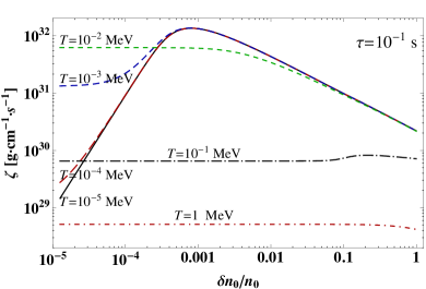
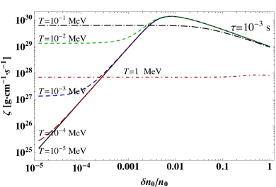
Figure 2: Bulk viscosity as a function of $\delta n_{0}/n_{0}$ for several fixed values of temperature, i.e. $T=10^{-5}~{}\mbox{MeV}$ (black solid line), $T=10^{-4}~{}\mbox{MeV}$ (red long-dashed line), $T=10^{-3}~{}\mbox{MeV}$ (blue dashed line), $T=10^{-2}~{}\mbox{MeV}$ (green short-dashed line), $T=10^{-1}~{}\mbox{MeV}$ (black dash-dotted line) and $T=1~{}\mbox{MeV}$ (red dash-dotted line line).

 

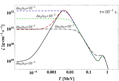
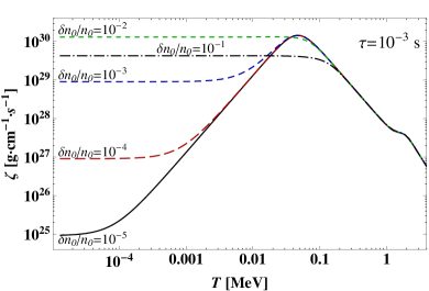
Figure 3: Bulk viscosity as a function of temperature for several fixed values of the amplitude of density oscillations, i.e. $\delta n_{0}/n_{0}=10^{-5}$ (black solid line), $\delta n_{0}/n_{0}=10^{-4}$ (red long-dashed line), $\delta n_{0}/n_{0}=10^{-3}$ (blue dashed line), $\delta n_{0}/n_{0}=10^{-2}$ (green short-dashed line), and $\delta n_{0}/n_{0}=10^{-1}$ (black dash-dotted line).

Here it is appropriate to mention that, in application to stellar quark matter, the bulk viscosity may not be the only, or even the dominant mechanism responsible for damping of the r-mode instabilities. For example, at sufficiently low temperatures, the corresponding dissipative dynamics is known to be dominated by the shear viscosity [7, 32]. (For several representative studies of the shear viscosity in dense quark matter see, for example, Refs. [33, 34, 35].) In this connection, our low-temperature results in Figs. 2 and 3 should be used only for the purpose of determining where exactly the damping by the shear viscosity takes over.

In order to better understand the role of nonlinear terms in the weak rates, see Eqs. (9) and (10), as well as their effect on the bulk viscosity, it is instructive to study the linear approximation. In this case, the expression for the viscosity can be derived analytically. As we shall see, this will be also helpful to elucidate the role of induced oscillations of $\delta\mu_{2}=\mu_{s}-\mu_{u}-\mu_{e}$ when the semileptonic processes are formally switched off.

3.1 Harmonic oscillations: linear approximation

In the linear regime, Eqs. (9) and (10) for dimensionless functions $\nu_{i}$ simplify down to

$$\frac{d\nu_{1}}{d\vartheta} = d_{1}\cos\vartheta-f_{1}\nu_{1}-f_{2}\nu_{2}+f_{3}(\nu_{2}-\nu_{1}),$$ (21)

$$\frac{d\nu_{2}}{d\vartheta} = d_{2}\cos\vartheta-h_{1}\nu_{1}-h_{2}\nu_{2}+h_{3}(\nu_{2}-\nu_{1}),$$ (22)

where $\vartheta=2\pi t/\tau$ is the dimensionless time variable, $d_{i}=C_{i}\delta n_{0}/(Tn_{0})$ is the magnitude of the “driving force”, and the other coefficient functions are

$$f_{1}=\lambda_{1}\frac{A_{1}}{\omega_{0}n_{0}},\qquad\qquad h_{1}=\lambda_{1}\frac{A_{2}}{\omega_{0}n_{0}},$$ (23)

$$f_{2}=\lambda_{2}\frac{A_{1}-B_{1}}{\omega_{0}n_{0}},\qquad\qquad h_{2}=\lambda_{2}\frac{A_{2}-B_{2}}{\omega_{0}n_{0}},$$ (24)

$$f_{3}=\lambda_{3}\frac{B_{1}}{\omega_{0}n_{0}},\qquad\qquad h_{3}=\lambda_{3}\frac{B_{2}}{\omega_{0}n_{0}}.$$ (25)

The general solution to this set of equations in the steady state regime is given by

$$\nu_{1} = x_{1}\cos\vartheta+y_{1}\sin\vartheta,$$ (26)

$$\nu_{2} = x_{2}\cos\vartheta+y_{2}\sin\vartheta,$$ (27)

where the coefficients satisfy the following set of algebraic equations:

$$(f_{1}+f_{3})x_{1}+(f_{2}-f_{3})x_{2}+y_{1} = d_{1},$$ (28)

$$-x_{1}+(f_{1}+f_{3})y_{1}+(f_{2}-f_{3})y_{2} = 0,$$ (29)

$$(h_{1}+h_{3})x_{1}+(h_{2}-h_{3})x_{2}+y_{2} = d_{2},$$ (30)

$$-x_{2}+(h_{1}+h_{3})y_{1}+(h_{2}-h_{3})y_{2} = 0.$$ (31)

It is straightforward, although tedious to solve this set of equations. When the solution is available, the result for the bulk viscosity will follow from Eq. (20), i.e.

$$\zeta = \frac{Tn_{0}^{2}}{\omega\delta n_{0}}\frac{A_{2}(C_{1}-C_{2})-B_{2}C_{1}}{A_{2}B_{1}-A_{1}B_{2}}x_{1}+\frac{Tn_{0}^{2}}{\omega\delta n_{0}}\frac{B_{1}C_{1}-A_{1}(C_{1}-C_{2})}{A_{2}B_{1}-A_{1}B_{2}}x_{2}.$$ (32)

It can be shown that this expression (with the appropriate solutions for $x_{1}$ and $x_{2}$) coincides exactly with the result for the bulk viscosity, obtained in Ref. [19].

3.2 Harmonic oscillations: nonleptonic contribution in linear approximation

If one ignores the semileptonic processes (i.e. if one formally takes $\lambda_{2}=\lambda_{3}=0$), the linearized equations (21) and (22) for $\nu_{i}$’s take the following form:

$$\frac{d\nu_{1}}{d\vartheta} = d_{1}\cos\vartheta-f_{1}\nu_{1},$$ (33)

$$\frac{d\nu_{2}}{d\vartheta} = d_{2}\cos\vartheta-h_{1}\nu_{1}.$$ (34)

The explicit solution to this set of equations in the steady state regime is given by

$$\nu_{1} = \frac{d_{1}}{1+f_{1}^{2}}\left(f_{1}\cos\vartheta+\sin\vartheta\right),$$ (35)

$$\nu_{2} = d_{2}\sin\vartheta+\frac{d_{1}h_{1}}{1+f_{1}^{2}}\left(\cos\vartheta-f_{1}\sin\vartheta\right),$$ (36)

and the corresponding expression for the bulk viscosity reads

$$\zeta_{\rm non} = \frac{Tn_{0}^{2}}{\omega\delta n_{0}}\frac{A_{2}(C_{1}-C_{2})-B_{2}C_{1}}{A_{2}B_{1}-A_{1}B_{2}}\frac{d_{1}f_{1}}{1+f_{1}^{2}}$$ (37)

$$+ \frac{Tn_{0}^{2}}{\omega\delta n_{0}}\frac{B_{1}C_{1}-A_{1}(C_{1}-C_{2})}{A_{2}B_{1}-A_{1}B_{2}}\frac{d_{1}h_{1}}{1+f_{1}^{2}}=\frac{\lambda_{1}C_{1}^{2}}{\omega^{2}+(\lambda_{1}A_{1}/n_{0})^{2}},$$

where we used the relation $f_{1}/h_{1}=A_{1}/A_{2}$ to arrive at the final result. As expected, this agrees with the known result [3, 13, 18, 19].

It is interesting to notice that the final result for the bulk viscosity receives a nonzero contribution due to the oscillation of $\nu_{2}\equiv\delta\mu_{2}/T$. Since $\delta\mu_{2}\equiv\mu_{s}-\mu_{u}-\mu_{e}$ controls the imbalance of the rates in the semileptonic processes, shown in Figs. 1 $(c)$ and $(d)$, which are formally switched off in the approximation at hand, one might wonder why there should be such a contribution at all. The answer is quite simple. In absence of the semileptonic processes the electron fraction in quark matter cannot change. However, when the nonleptonic processes drive the oscillations of the strangeness composition, they inevitably induce the oscillations of $\delta\mu_{2}\equiv\mu_{s}-\mu_{u}-\mu_{e}$. Then, the latter contributes to the instantaneous pressure and, in turn, to the bulk viscosity. Interestingly, such a contribution due to the induced oscillation of $\nu_{2}\equiv\delta\mu_{2}/T$ were ignored in all previous studies [3, 12, 13, 14, 15, 16, 17, 18]. Fortunately, the corresponding correction is quantitatively small. The reason for its smallness seems to be rooted in the “accidental” fact that one of the susceptibility functions, $B_{2}$, is inversely proportional to the square of the chemical potential of electrons (rather than quarks) and, thus, is considerably larger than all others [19].

4 Bulk viscosity in anharmonic regime

In this section we study the effect that anharmonic oscillations of the density have on the bulk viscosity of dense quark matter.

4.1 Anharmonic oscillations of Type I

Let us start by modeling the density oscillations of quark matter $\delta n(t)$ by a time dependent anharmonic function of Type I, which is a solution to Eq. (3) with a fixed anharmonicity parameter $\alpha^{*}$. Before we proceed to the numerical results, it is important to notice that the corresponding oscillations are asymmetric with respect to the equilibrium point $\delta n_{\rm eq}=0$. For $\alpha^{*}<0$, the density oscillations are larger in the direction of positive $\delta n$, while for $\alpha^{*}>0$, the oscillations are larger in the direction of negative $\delta n$, see also Fig. 5. The cases of the positive and negative anharmonicity parameters are physically equivalent, however. Indeed, they are related by the following sign reversal symmetry: $\alpha\to-\alpha$ and $\delta n\to-\delta n$. Therefore, it is sufficient to study only one of them. For technical reasons, we choose $\alpha^{*}<0$.

 

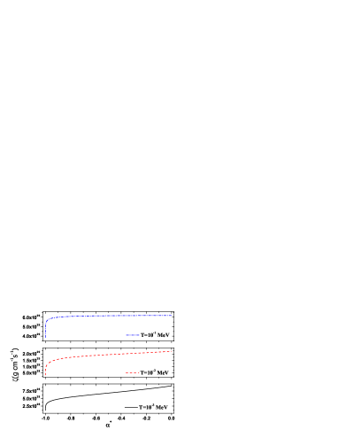
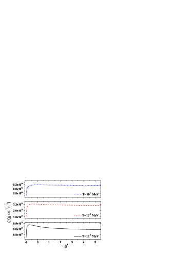
Figure 4: Bulk viscosity as a function of anharmonicity parameter of Type I (left panel) and Type II (right panel) for $\tau=10^{-3}~{}\mbox{s}$, $\delta n_{0}/n_{0}=10^{-3}$ and several representative values of temperature.

Typical results for the bulk viscosity as a function of anharmonicity parameter $\alpha^{*}$ are shown in the left panel of Fig. 4 for the whole range of negative $\alpha^{*}$, i.e. $-1<\alpha^{*}<0$, for which physically meaningful periodic solutions exist. We used the following values of the period and the amplitude of density oscillations: $\tau=10^{-3}~{}\mbox{s}$ and $\delta n_{0}/n_{0}=10^{-3}$, and plotted the results for several representative values of temperature. [It should be emphasized that the period $\tau$ is related to the “bare” frequency $\omega_{0}$ by a modified relation, see Eq. (40).] In general, we find that the bulk viscosity decreases with increasing the degree of anharmonicity. This qualitative behavior may be understood as the result of an effective increase of the frequency of oscillations due to an admixture of higher harmonics. Quantitatively, however, the effect is rather small. Only a very large anharmonicity ($\alpha^{*}\approx-1$) leads to a substantial decrease of the bulk viscosity.

4.2 Anharmonic oscillations of Type II

Anharmonic density oscillations of Type II are modeled by a function $\delta n(t)$, which is a solution to Eq. (4) with a fixed anharmonicity parameter $\beta^{*}$. Conceptually, this is a simpler case because the oscillations are symmetric about the equilibrium point $\delta n_{\rm eq}=0$. Unlike the case of Type I oscillations, there is no reversal symmetry here. As in the previous case, however, periodic solution exist only for a range of values of the the anharmonicity parameter, $\beta^{*}>-1$.

Numerical results for the bulk viscosity as a function of anharmonicity parameter $\beta^{*}$ are shown in the right panel of Fig. 4. The qualitative dependence of the viscosity on the parameter $\beta^{*}$ is somewhat different. While it decreases at large values of parameter $\beta^{*}$, there is a range of small negative values of $\beta^{*}$, where it slightly grows with increasing anharmonicity. Moreover, this feature seems to be rather general and especially pronounced in the nonlinear regime (small temperature). Just like in the case of Type I oscillations, the effects appear to be rather small.

5 Discussion

In this paper we studied the bulk viscosity of dense quark matter by taking into account the nonlinear dependence of the nonleptonic and semileptonic weak rates on the parameter $\delta\mu_{i}/T$, where $\delta\mu_{i}$ are the chemical potential imbalances that control the departure of strange quark matter from $\beta$ equilibrium. We reproduce the earlier obtained interplay of the nonleptonic and semileptonic processes, leading to an increase (“hump”) of the viscosity in a narrow temperature range around $1~{}\mbox{MeV}$. The nonlinear corrections have a small effect on the corresponding shape of the “hump”. The reason for this is a relatively high temperature ($T\sim 1~{}\mbox{MeV}$), at which the corresponding effects can occur. At such moderately high temperatures, the interplay between the two types of weak processes is substantially affected only if the nonlinearity (measured by $\delta n_{0}/n_{0}$) is well above $10\%$.

In this study, we also found that the anharmonicity of density oscillations has an effect on the bulk viscosity, even though the effect was not large in the cases that we studied. For a strong anharmonicity, the bulk viscosity showed a substantial decrease. We also saw that different types of anharmonicity have slightly different qualitative as well as quantitative outcomes. This finding may suggest that some types of anharmonicity may be more efficient and, thus, lead to larger corrections to the bulk viscosity. In this preliminary study, we considered only a toy model to introduce the anharmonic oscillations. In the future, it may be interesting to study more realistic types of density oscillations that result from the actual nonlinear dynamics of stellar r-modes, produced by the gravitational emission.

Here we studied the bulk viscosity only in the normal phase of dense quark matter. One may wonder, however, how the results will be modified if quark matter is a color superconductor [36]. As suggested by several existing studies in the linear regime, color superconductivity can have a large effect on the bulk viscosity [20, 28, 37, 38]. The additional effects due to the nonlinear regime may be much harder to predict. One of the complications comes from the fact that the weak rates in color superconducting matter have a strong dependence on the ratio of the superconducting energy gap and temperature, $\phi/T$. Moreover, in the suprathermal regime, their dependence on $\delta\mu_{i}/T$ will most likely be nonpolynomial. These technical difficulties can be resolved in principle, but the outcome is not obvious and the corresponding study is outside the scope of the present paper.

Appendix A Anharmonic oscillator

A.1 Anharmonic oscillator with a cubic potential (Type I)

The anharmonic oscillator with cubic potential $U(x)=m\omega_{0}^{2}\left(\frac{x^{2}}{2}+\alpha\frac{x^{3}}{3}\right)$ is described by the following equation of motion:

$$\ddot{x}+\omega_{0}^{2}x\left(1+\alpha x\right)=0.$$ (38)

By making use of the known parametric solution to the above differential equation [39] and assuming that $x_{0}>0$ is the maximum deviation from the equilibrium point $x=0$ in the positive $x$-direction, we find that the periodic solution exists for $-1<\alpha x_{0}<1/2$. (The apparent asymmetry between positive and negative values of $\alpha x_{0}$ is a result of the assumption that $x_{0}$ is the maximum deviation from the equilibrium point in the positive $x$-direction.) It is given in terms of the Jacobi elliptic function $\mbox{sn}\left(u|m\right)$ as follows:

$$x(t)=x_{0}\left[1-\frac{3a_{-}}{2\alpha^{*}}\mbox{sn}\left(\frac{(t-t_{0})\omega_{0}\sqrt{a_{+}}}{2}\Big{|}\frac{a_{-}}{a_{+}}\right)^{2}\right],$$ (39)

where $a_{\pm}=\frac{1}{2}\left(1+2\alpha^{*}\pm\sqrt{(1+\frac{2}{3}\alpha^{*})(1-2\alpha^{*})}\right)$ and $\alpha^{*}\equiv\alpha x_{0}$ is a dimensionless parameter that measures the maximum deviation of the solution from the harmonic regime. Note that $x(t)$ is periodic with the period given by

$$\tau_{\alpha} = \frac{4}{\omega_{0}\sqrt{a_{+}}}K\left(\frac{a_{-}}{a_{+}}\right)$$ (40)

$$\simeq \frac{2\pi}{\omega_{0}}\left(1+\frac{5}{12}(\alpha\,x_{0})^{2}+\frac{5}{18}(\alpha\,x_{0})^{3}+O\left[(\alpha\,x_{0})^{4}\right]\right),~{}\mbox{for}~{}~{}\alpha\,x_{0}\to 0,$$

where $K\left(a_{-}/a_{+}\right)$ is the complete elliptic integral of the first kind. Two representative solutions are shown in Fig. 5.

 

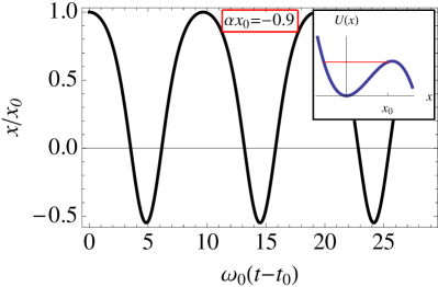
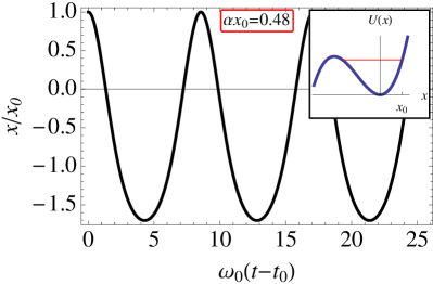
Figure 5: Solutions to the equation of motion of the anharmonic oscillator with a cubic potential for two values of the coupling constant. The inserts show the corresponding shapes of the potentials.

For anharmonic solutions of this type, the average kinetic energy is given by

$$\langle E_{\rm kin}\rangle=\frac{1}{\tau_{\alpha}}\int_{0}^{\tau_{\alpha}}\frac{m\dot{x}^{2}}{2}dt=\frac{m\omega_{0}^{2}x_{0}^{2}}{4}{\cal F},$$ (41)

where the analytical expression for constant ${\cal F}$ reads

$${\cal F}=\frac{4(1+\alpha^{*})}{5\alpha^{*}a_{-}}\left\{\frac{E\left(\frac{a_{-}}{a_{+}}\right)}{K\left(\frac{a_{-}}{a_{+}}\right)}-(a_{+}-a_{-})\left(a_{+}-\frac{1}{2}a_{-}\right)\right\}.$$ (42)

Here $E\left(a_{-}/a_{+}\right)$ is the complete elliptic integral of the second kind.

A.2 Anharmonic oscillator with a quartic potential (Type II)

The anharmonic oscillator with quartic potential $U(x)=m\omega_{0}^{2}\left(\frac{x^{2}}{2}+\beta\frac{x^{4}}{4}\right)$ is described by the following equation of motion:

$$\ddot{x}+\omega_{0}^{2}x\left(1+\beta x^{2}\right)=0,\qquad(\mbox{Type II}).$$ (43)

Using the known parametric solution to the above differential equation [39] and assuming that $x_{0}$ is the maximum deviation from the equilibrium point $x=0$, we find that the periodic solution exists for $\beta^{*}\equiv\beta\,x_{0}^{2}>-1$. The solution is given in terms of the Jacobi elliptic function,

$$x(t) = x_{0}\frac{\sqrt{1+(1/2)\beta^{*}}}{\sqrt{1+\beta^{*}}}\,\mbox{sd}\left(\omega_{0}(t-t_{0})\sqrt{1+\beta^{*}}\Big{|}\frac{\beta^{*}}{2(1+\beta^{*})}\right).$$ (44)

This is a periodic solution with the period equal

$$\tau_{\beta} = \frac{4}{\omega_{0}\sqrt{1+\beta^{*}}}\,K\left(\frac{\beta^{*}}{2(1+\beta^{*})}\right)$$ (45)

$$\simeq \frac{2\pi}{\omega_{0}}\left(1-\frac{3}{8}\beta\,x_{0}^{2}+\frac{57}{256}\beta^{2}\,x_{0}^{4}+O\left(\beta^{3}\,x_{0}^{6}\right)\right),\quad\mbox{for}\quad\beta\,x_{0}^{2}\to 0.$$

Two representative solutions are shown in Fig. 6.

 

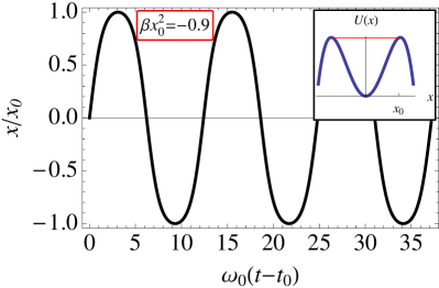
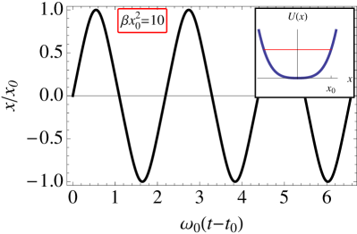
Figure 6: Solutions to the equation of motion of the anharmonic oscillator with a quartic potential for two values of the coupling constant. The inserts show the corresponding shapes of the potentials.

For solutions of this type, the average kinetic can be given in the same form as in Eq. (41), but the value of the corresponding constant ${\cal F}$ is different,

$${\cal F}=\frac{4(1+\beta^{*})}{3\beta^{*}}\left\{1+\frac{\beta^{*}}{2}-\frac{E\left(\frac{\beta^{*}}{2(1+\beta^{*})}\right)}{K\left(\frac{\beta^{*}}{2(1+\beta^{*})}\right)}\right\}.$$ (46)

References

References

- [1] P. Demorest, T. Pennucci, S. Ransom, M. Roberts and J. Hessels, Nature 467, 1081 (2010).
- [2] F. Özel, D. Psaltis, S. Ransom, P. Demorest and M. Alford, Astrophys. J. Lett. 724, L199 (2010).
- [3] J. Madsen, Phys. Rev. D 46, 3290 (1992).
- [4] L. Lindblom, B. J. Owen and S. M. Morsink, Phys. Rev. Lett. 80, 4843-4846 (1998).
- [5] B. J. Owen, L. Lindblom, C. Cutler, B. F. Schutz, A. Vecchio and N. Andersson, Phys. Rev. D 58, 084020 (1998).
- [6] L. Lindblom, G. Mendell and B. J. Owen, Phys. Rev. D 60, 064006 (1999).
- [7] J. Madsen, Phys. Rev. Lett. 85, 10 (2000).
- [8] S. Chandrasekhar, Phys. Rev. Lett. 24, 611 (1970).
- [9] J. L. Friedman and B. F. Schutz, Astrophys. J. 222, 281 (1978).
- [10] N. Andersson, Astrophys. J. 502, 708 (1998).
- [11] J. L. Friedman and S. M. Morsink, Astrophys. J. 502, 714-720 (1998).
- [12] Q. D. Wang and T. Lu, Phys. Lett. B 148, 211 (1984).
- [13] R. F. Sawyer, Phys. Lett. B 233, 412 (1989).
- [14] X. P. Zheng, S. H. Yang and J. R. Li, Phys. Lett. B 548, 29-34 (2002).
- [15] Z. Xiaoping, L. Xuewen, K. Miao and Y. Shuhua, Phys. Rev. C 70, 015803 (2004).
- [16] H. Dong, N. Su and Q. Wang, Phys. Rev. D 75, 074016 (2007).
- [17] X.-G. Huang, M. Huang, D. H. Rischke and A. Sedrakian, Phys. Rev. D 81, 045015 (2010).
- [18] M. G. Alford, S. Mahmoodifar and K. Schwenzer, J. Phys. G 37, 125202 (2010).
- [19] B. A. Sa’d, I. A. Shovkovy and D. H. Rischke, Phys. Rev. D 75, 125004 (2007).
- [20] X. Wang and I. A. Shovkovy, Phys. Rev. D 82, 085007 (2010).
- [21] A. Reisenegger and A. A. Bonacic, astro-ph/0303454.
- [22] T. Van Hoolst, Astron. Astrophys. 308, 66 (1996).
- [23] N. Stergioulas and J. A. Font, Phys. Rev. Lett. 86, 1148 (2001).
- [24] L. Lindblom, J. E. Tohline and M. Vallisneri, Phys. Rev. Lett. 86, 1152 (2001).
- [25] A. K. Schenk, P. Arras, E. E. Flanagan, S. A. Teukolsky and I. Wasserman, Phys. Rev. D 65, 024001 (2002).
- [26] P. Arras, E. E. Flanagan, S. M. Morsink, A. K. Schenk, S. A. Teukolsky and I. Wasserman, Astrophys. J. 591, 1129 (2003).
- [27] M. Gabler, U. Sperhake and N. Andersson, Phys. Rev. D 80, 064012 (2009).
- [28] B. A. Sa’d, I. A. Shovkovy and D. H. Rischke, Phys. Rev. D 75, 065016 (2007).
- [29] P. Haensel, Astron. Astrophys. 262, 131 (1992).
- [30] A. Reisenegger, Astrophys. J. 442, 749 (1995).
- [31] J. Madsen, Phys. Rev. D 47, 325 (1993).
- [32] P. Jaikumar, G. Rupak and A. W. Steiner, Phys. Rev. D 78, 123007 (2008).
- [33] H. Heiselberg and C. J. Pethick, Phys. Rev. D 48, 2916 (1993).
- [34] C. Manuel, A. Dobado and F. J. Llanes-Estrada, JHEP 0509, 076 (2005).
- [35] M. G. Alford, M. Braby and S. Mahmoodifar, Phys. Rev. C 81, 025202 (2010).
- [36] M. G. Alford, A. Schmitt, K. Rajagopal and T. Schäfer, Rev. Mod. Phys. 80, 1455 (2008).
- [37] M. G. Alford and A. Schmitt, J. Phys. G 34, 67 (2007).
- [38] M. G. Alford, M. Braby and A. Schmitt, J. Phys. G 35, 115007 (2008).
- [39] A. D. Polyanin and V. F. Zaitsev, Handbook of exact solutions for ordinary differential equations, Second Edition, (Chapman and Hall, 2002), p. 318.