Temperature distribution of a non-flaring active region from simultaneous Hinode XRT and EIS observations

Abstract

We analyze coordinated Hinode XRT and EIS observations of a non-flaring active region to investigate the thermal properties of coronal plasma taking advantage of the complementary diagnostics provided by the two instruments. In particular we want to explore the presence of hot plasma in non-flaring regions. Independent temperature analyses from the XRT multi-filter dataset, and the EIS spectra, including the instrument entire wavelength range, provide a cross-check of the different temperature diagnostics techniques applicable to broad-band and spectral data respectively, and insights into cross-calibration of the two instruments.

The emission measure distribution, $EM(T)$, we derive from the two datasets have similar width and peak temperature, but show a systematic shift of the absolute values, the EIS $EM(T)$ being smaller than XRT $EM(T)$ by approximately a factor 2. We explore possible causes of this discrepancy, and we discuss the influence of the assumptions for the plasma element abundances. Specifically, we find that the disagreement between the results from the two instruments is significantly mitigated by assuming chemical composition closer to the solar photospheric composition rather than the often adopted “coronal” composition (Feldman, 1992).

We find that the data do not provide conclusive evidence on the high temperature ($\log T[{\rm K}]\gtrsim 6.5$) tail of the plasma temperature distribution, however, suggesting its presence to a level in agreement with recent findings for other non-flaring regions.

1. Introduction

Understanding how solar and stellar coronae are heated to high temperatures is one of the most important open issues in astrophysics. Coronal heating is clearly related to the strong magnetic fields that fill the atmospheres of the Sun and solar-like stars, but the mechanism that converts magnetic energy into thermal energy remains unknown. Theoretical models based on steady heating failed to explain the physical properties observed in coronal structures. A promising and widely studied framework for understanding coronal heating is the nanoflare model proposed by Parker (1972). In this model, convective motions in the photosphere lead to the twisting and braiding of coronal magnetic field lines. This topological complexity ultimately leads to the formation of current sheets, where the magnetic field can be rearranged through the process of magnetic reconnection. This model has been further refined and adapted to a scenario where nanoflares occur in unresolved strands in coronal loops, below the spatial resolution of available instrumentation (Parker, 1988; Cargill, 1994; Cargill & Klimchuk, 1997; Klimchuk, 2006; Warren et al., 2003; Parenti et al., 2006).

Nanoflare models predict the presence of very hot plasma with temperatures in excess of 3 MK in non flaring solar regions; depending on the energy of the nanoflare, temperatures may reach or even exceed 10 MK. Unambiguous detection of such extreme temperatures in non-flaring solar regions can provide convincing evidence for the presence of nanoflares. However, such detection is not easy, as the amount of very hot plasma produced by nanoflares is expected to be very small. Recent studies have provided some evidence of the presence of hot plasma in the non-flaring Sun. McTiernan (2009) carried out an analysis of the temperature and emission measure determined from quiescent plasma during the 2002-2006 decay phase of solar cycle 23, as derived from GOES and RHESSI observations. He found a persistent faint plasma component with temperatures approximately constant during the entire 2002-2006 interval, and approximately between 5 and 10 MK. However, GOES and RHESSI provided different values of such temperature, and their results were not necessarily well correlated; also, this analysis relied on the isothermal plasma assumption.

Other studies tried to identify the hot plasma through the X-ray emission observed by the X-ray Telescope (XRT; Golub et al., 2007) onboard Hinode (Kosugi et al., 2007). Reale et al. carried out a temperature analysis of a non-flaring active region, first with only XRT multi-filter data (Reale et al., 2009b) and then combining XRT and RHESSI observations (Reale et al., 2009a). Their findings point to the presence of small amounts of very hot plasmas, with temperatures of $\simeq 5-10$ MK, and emission measure of the order of few percent of the dominant cool component. These characteristics of the emission measure distribution are compatible with the predictions of nanoflare models. However, they spelled out and discussed the main limitations of their study and similar analyses. First, XRT is also sensitive to plasma at normal active region temperatures (2-3 MK) and thus contamination from the colder active region plasma is a considerable obstacle to the detection of the much smaller amounts of hot plasma; also, the limited temperature resolution of XRT prevents a detailed study of the cold component. Second, RHESSI sensitivity makes it very hard to even detect the quiescent active region plasma. Third, instrumental calibration is an issue for both instruments. Schmelz et al. (2009b) also detected a faint hot temperature tail to the emission measure distribution of active region plasma, and determined its temperature to be around 30 MK. Subsequent analyses by Schmelz et al. (2009a) included RHESSI data and, while confirming the presence of such hot material, could not reconcile the XRT and RHESSI observations using the standard calibration of both instruments. A self-consistent solution was only found if a series of instrumental parameters and the plasma element abundances were adjusted, and the temperature of the hot plasma decreased.

Ample efforts have been devoted to the accurate determination of the thermal structuring of coronal plasma to derive robust observational constraints to the mechanism(s) of coronal heating. The plasma temperature distribution of the quiet corona and of active regions has been investigated through imaging data and spectroscopic observations (e.g., Brosius et al., 1996; Landi & Landini, 1998; Aschwanden et al., 2000; Testa et al., 2002; Del Zanna & Mason, 2003; Reale et al., 2007; Landi et al., 2009; Shestov et al., 2010; Sylwester et al., 2010). Several recent works have focused on EUV spectra obtained with the Hinode Extreme Ultraviolet Imaging Spectrometer (EIS; Culhane et al. 2007 ) which provides good temperature diagnostic capability, together with higher spatial resolution and temporal cadence than previously available (e.g., Watanabe et al., 2007; Warren et al., 2008; Patsourakos & Klimchuk, 2009; Brooks et al., 2009; Warren & Brooks, 2009).

In the present work, we address the issue of determining the temperature distribution of coronal plasma from a different perspective: we investigate thermal properties of coronal plasma in non-flaring active regions using simultaneous Hinode observations with XRT and with EIS, which provide complementary diagnostics for the X-ray emitting plasma. The multi-filter XRT dataset together with EIS spectra, including its entire wavelength range, allow to accurately determine the thermal structure of the active region plasma, and to explore the presence of hot plasma in non-flaring regions. We use spectroscopic observations from the Hinode/EIS instrument of a quiescent active region to constrain the emission measure distribution of the bulk of the active region plasma with the spectral lines observed by EIS in the 171-212Å and 245-291Å spectral ranges (see also e.g., Young et al. 2007; Doschek et al. 2007). Since EIS is most sensitive to plasma with temperatures of 0.6-2 MK, EIS spectra allow us to accurately determine the emission measure distribution of the quiescent active region plasma, to evaluate the fraction of the observed XRT count rates that it emits, and thus investigate the true amount of emission from the nanoflaring plasma. Thus, the combination of XRT and EIS observations of the same active region allows us to characterize the plasma temperature distribution with better detail than in previous studies. In fact, while some previous studies have made use of data from both imaging and spectroscopic data to constrain the properties of the emitting plasma (e.g., Warren et al., 2010; Landi et al., 2010; O’Dwyer et al., 2010), to our knowledge no previous work has carried out a determination of the temperature distribution by combining XRT and EIS data, nor a quantitative comparison of the independent analysis from the different instruments, as we do here. Independent temperature analysis from the two datasets provide a cross-check of the different temperature diagnostics techniques applicable to spectral and broad-band data respectively, and insights into cross-calibration of the two instruments.

The observations are described in Section 2. The data analysis and results of the determination of the plasma temperature distribution are presented in Section 3. Our findings are discussed in Section 4 and summarized in Section 5.

2. Observations

Table 1Details of Hinode XRT and EIS observations analyzed in this paper, and shown in Figures 1, and 2.

	XRT						EIS
	Al-poly	C-poly	Ti-poly	Be-thin	Be-med	Al-med	171-212Å, 245-291Å
FOV	384′′$\times$384′′						128′′$\times$128′′
START OBS	2008-06-20T23:27:30						2008-06-20T23:03:39
END OBS	2008-06-21T03:38:50						2008-06-21T02:19:14
$t_{\rm exp}$ [s]	4.1	8.2	8.2	23	33	46	90

We observed the non-flaring NOAA active region 10999 close to disk center, beginning on June 20 2008 around 23 UT for several hours with both the X-ray Telescope and the Extreme Ultraviolet Imaging Spectrometer onboard Hinode. The details of the observations are presented in Table 1.

XRT observed AR 10999 in several filters, with a field of view (FOV) of 384^′′$\times$384^′′, for about 4 hours starting June 20 2008 at 23:27 UT, with a cadence of about 5 minutes in each filter. We analyze observations in the following filters: Al_poly, C_poly, Ti_poly, Be-thin, Be-med, Al-med. The XRT data were processed with the standard routine xrt_prep, available in SolarSoft to remove the CCD dark current, and cosmic-ray hits. Figure 1 shows the images of XRT observations in Al-poly, Be-thin and Be-med, integrated over the entire observing time (see also Table 1 for details).

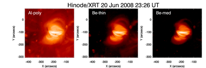
Figure 1.— XRT images of AR 10999, obtained summing all the images taken in a given filter over the $\sim 3$ hr observation (see Table 1): Al-poly (left; total integration time $t_{\rm int}\sim 131$ s), Be-thin (center; $t_{\rm int}\sim 828$ s), and Be-med filter (right; $t_{\rm int}\sim 1155$ s).

The FOV of the EIS observations analyzed here is 128^′′$\times$128^′′ and was built up by stepping the 1^′′ slit from solar west to east over a 3.5 hr period from 23:03 UT of June 20th to 02:19 UT of June 21st. The study includes full spectra on both the EIS detectors from 171-212Å and 245-291Å. The exposure time was 90 s and the study acronym is HPW001_FULLCCD_RAST. The observations were carried out during eclipse season and they were not paused during eclipses: the black stripes of missing data in Figure 2 correspond to Hinode eclipses. The EIS data are processed with the eis_prep routine available in SolarSoft to remove the CCD dark current, cosmic-ray strikes on the CCD, and take into account hot, warm, and dusty pixels. In addition, the radiometric calibration is applied to convert the data from photon events to physical units. The EIS routine eis_ccd_offset is then used to correct for the wavelength dependent relative offset of the two CCDs of 1-2 pixels in the X-direction, and $\sim 18$ pixels in the Y-direction. Figure 2 shows images obtained from EIS observations by integrating over narrow wavelength ranges each dominated by a single line with different characteristic temperature of formation. We also show three small areas of the active region which have been selected for the detailed analysis of thermal structuring (see next section for details).

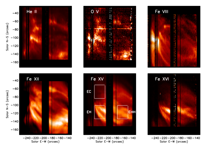
Figure 2.— EIS images in spectral lines formed at different characteristic plasma temperatures: He ii (256.32Å, $\log(T_{\rm max}[{\rm K}])=4.9$), O v (248.46Å, $\log(T_{\rm max}[{\rm K}])=5.4$), Fe viii (185.21Å, $\log(T_{\rm max}[{\rm K}])=5.55$), Fe xii (195.12Å, $\log(T_{\rm max}[{\rm K}])=6.15$), Fe xv (284.16Å, $\log(T_{\rm max}[{\rm K}])=6.35$), Fe xvi (262.98Å, $\log(T_{\rm max}[{\rm K}])=6.4$). In the 284Å Fe xv image we indicate the three regions selected for the analysis of the plasma thermal structure (see Figure 4 and §3): EC (top left), EH (bottom left), EHH (bottom right).

3. Analysis Methods and Results

Inspection of the XRT observations, in all filters, indicate that the active region is characterized by a modest level of variability over a wide range of temperatures (see Figure 3). Therefore, in order to increase S/N, we have analyzed the XRT dataset obtained by coaligning the images taken in each filter at different times, and then summing them up.

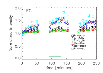
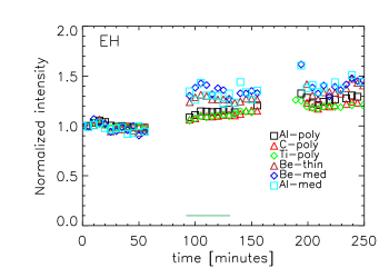
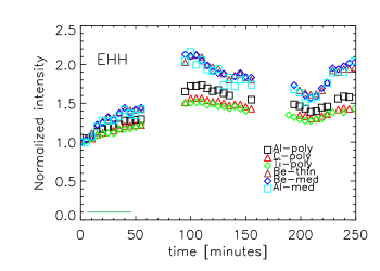
Figure 3.— Lightcurves of XRT observations in all analyzed filters, for the three selected regions: EC (top), EH (middle), EHH (bottom). For each filter the signal is normalized to the intensity in the first image. The solid line at the bottom of the plot indicates the time interval when EIS was observing the selected region.

In order to carry out a direct and detailed comparison of thermal analysis from XRT and EIS data, we have then selected a few subregions. To select these regions we have first obtained maps of temperature and emission measure over the whole active region, by using estimates derived with the so-called combined improved filter ratio method, devised by Reale et al. (2007). The resulting temperature map is shown in Figure 4. We selected three regions, of area approximately 30^′′$\times$30^′′: EC, which in the temperature map homogeneously appears as relatively cool, and two hotter regions (EH, EHH). The values of temperature mean and standard deviation derived for these three regions from the CIFR diagnostics are: $1.5\pm 0.1$ MK (EC), $1.9\pm 0.2$ MK (EH), and $2.0\pm 0.2$ MK (EHH). When selecting the boundaries of region EHH in the XRT data, we slightly modified the shape (however maintaining the area value) in order to avoid the contamination spots clearly visible in the temperature map as bright blobs immediately to the east and north of the selected area. Figure 2 shows the selected regions in the EIS Fe xv 284Å image. For the temperature analysis presented in the rest of the paper we integrated the XRT and EIS signals over each of these regions, over the time intervals when the two instruments were simultaneously observing the selected region. Figure 3 shows that the XRT light curves of each region changed little over the time period when EIS was observing the same areas.

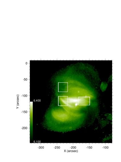
Figure 4.— Temperature map obtained from the combined improved filter ratio from the XRT images of AR 10999 shown in Figure 1. The three regions selected for the detailed temperature analysis are indicated: EC (top left), EH (bottom left), EHH (bottom right). When selecting the boundaries of region EHH we modified the shape (however maintaining the area value) in order to avoid the contamination spots clearly visible in the temperature map as bright blobs immediately to the east and north of the selected area.

Figure 5 shows the EIS full spectra in the three regions selected for the analysis, with the identification of the brightest lines. The EIS exposure time (90 s at each location) yields high signal in the strongest lines, mostly produced in a temperature range $\log T[{\rm K}]\sim 5.8-6.3$. Hotter lines present in the EIS wavelength range have generally low intensities, in typical solar non-flaring conditions, and are difficult to detect. We have selected a list of lines which are suitable for an accurate derivation of the plasma thermal properties. This list (see Table 2) includes strong lines, unblended and with reliable atomic data, and we also included hot lines for which however we can only derive upper limits from the EIS observations of this non-flaring active region. These upper limits are nevertheless useful to constrain the high temperature component ($\log T[{\rm K}]\gtrsim 6.5$).

Figure 5.— EIS spectra of the three regions selected for the analysis: EC (top), EH (middle), EHH (bottom). The identification of the spectral lines used for the analysis of the plasma thermal properties (listed in Table 2) are shown in the spectrum in the top panel.

Table 2Identification and measured fluxes of EIS spectral lines used for reconstructing the DEM of the three regions selected for the analysis and shown in Figure 2.

$\lambda$ [Å]	Ion	$\log(T_{\rm max}[{\rm K}])$	flux [erg cm-2 s-1]			Notes
			EC	EH	EHH
171.0755	Fe xix	5.9	8494.52	16757.8	9238.51
174.5340	Fe x	6.0	7310.57	12152.6	7888.11
177.2430	Fe x	6.0	4231.15	7555.12	4736.85
180.4080	Fe xi	6.1	10609.4	16354.4	11523.8
182.1690	Fe xi	6.1	1784.80	3021.49	1914.51
186.8520	Fe xii	6.2	694.141	1099.68	426.001
186.8840	Fe xii	6.2	3129.81	5212.59	3902.01
188.2320	Fe xi	6.1	5613.69	8863.01	6469.60
192.0285	Fe xxiv	7.3	310.929	539.337	304.685	u
192.3930	Fe xii	6.2	4107.59	5858.81	4550.20
195.1180	Fe xii	6.2	14092.9	21301.2	16415.0
202.0440	Fe xiii	6.2	11240.2	15845.5	14868.5
204.6542	Fe xvii	6.7	37.2628	60.1331	44.5043	u
208.6040	Ca xvi	6.7	5.61904	17.4814	38.7130	u
246.0200	Si vi	5.6	76.5847	91.3415	28.2609
249.1240	Si vi	5.6	29.2495	38.8003	15.6522
249.1780	Ni xvii	6.5	20.5272	277.752	312.949
253.1702	Fe xxii	7.1	3.55755	9.38507	9.47460	u
253.7880	Si x	6.1	379.199	578.696	436.514
258.3710	Si x	6.1	2737.30	4175.65	3144.01
261.0440	Si x	6.1	1151.82	1731.62	1318.26
262.9760	Fe xvi	6.4	173.934	968.696	1036.80
263.7657	Fe xxiii	7.2	14.5618	12.5289	9.42194	u
264.2310	S x	6.2	925.718	975.778	899.526
264.7900	Fe xiv	6.3	2784.31	5570.13	4768.17
265.0010	Fe xvi	6.4	19.6691	105.484	99.7671
270.5220	Fe xiv	6.3	1356.52	3060.05	2607.03
272.0060	Si x	6.1	1117.27	1592.69	1191.82
272.6390	Si vii	5.8	134.686	237.159	99.4883
275.3540	Si vii	5.8	456.285	706.011	317.491
284.1630	Fe xv	6.3	10317.8	28644.9	27965.3

In the following we will describe in detail the analysis methods and results obtained for one of the selected regions, EHH. Then we will discuss our findings for all three regions.

3.1. Thermal Structuring from EIS spectra

For the analysis of EIS spectra and XRT data, we use the Package for Interactive Analysis of Line Emission (PINTofALE, Kashyap & Drake 2000) which is available on SolarSoft. For the spectral analysis and emission measure distribution reconstruction from EIS spectra we use CHIANTI v.6.0.1 (Dere et al., 1997, 2009), with the ionization balance of Bryans et al. (2009). Unless explicitly stated otherwise we assume “coronal” plasma abundances of Feldman (1992).

The observed line intensities provide constraints on the plasma temperature distribution, as they depend on the plasma emissivities $G_{\lambda}(T,n)$, element abundances $A_{Z}$, and differential emission measure distribution $DEM(T)$:

$$I_{\lambda}=A_{Z}\int_{T}G_{\lambda}(T,n_{e})DEM(T)\,dT$$ (1)

where $DEM(T)=n_{e}^{2}\,dV/dT$ $[{\rm cm}^{-3}{\rm K}^{-1}]$.

Several lines listed in Table 2 are density sensitive, so it is necessary to measure the electron density of the emitting plasma for each region before calculating the contribution functions to be used in the analysis. We have used the line intensity ratios of Si x, Fe xii and Fe xiv available in the dataset, and the results are listed in Table 3. The most reliable indicator of the electron density is Si x, since its lines are not affected by blends and have been found to be reliable by Young et al. (1998) and Landi et al. (2002). The Fe xiv intensity ratio is less sensitive to the electron density and provides a much coarser estimate; the density values it indicates are broadly consistent with the Si x measurements. The Fe xii densities, while consistent within the uncertainties, are a bit larger than those of Si x, a behavior that has already been noted elsewhere (Young et al., 2009; Watanabe et al., 2009); this might be due to atomic physics problems affecting the Fe xii emissivities (however, see also Tripathi et al. 2010). Throughout the present work, we used $\log n_{e}=9.0$ for all regions in the calculation of the spectral emissivities from CHIANTI.

Table 3Electron density diagnostic results for each region. The density adopted throughout the study is $\log n_{e}=9.0$. Densities are in cm^-3.

Ion	Line ratio	$\log n_{e}$
		EC	EH	EHH
Si x	261.0/253.8	8.95${}^{+0.30}_{-0.20}$	9.00$\pm$0.25	8.95${}^{+0.30}_{-0.20}$
Fe xii	186.8/195.1	9.15${}^{+0.15}_{-0.20}$	9.20$\pm$0.20	9.10$\pm$0.15
Fe xiv	264.8/270.5	9.5$\pm$0.4	9.3${}^{+0.3}_{-0.5}$	9.3${}^{+0.3}_{-0.5}$

Figure 6 shows the EM loci corresponding to the fluxes measured for one of the regions. The curves represent the loci of constant flux for a given line, i.e. they are obtained by taking the ratio of the measured line flux to the emissivity function (including the element abundance) of that line. The EM loci plot provides a visual indication of the temperature range covered by the selected lines and passbands, since we are also including EM loci for the XRT observations. For the XRT channels the EM loci are derived by dividing the measured fluxes by the temperature response of that channel, derived assuming a given set of element abundances (in the case of Fig. 6 we use coronal abundances). Also, if the underlying plasma were isothermal the EM loci curves would all cross at a single points, therefore this plot also provides some indication for the characteristics of temperature distribution of the plasma.

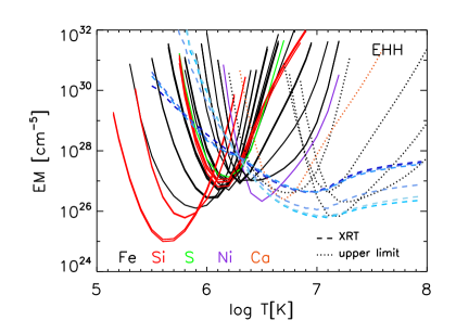
Figure 6.— EM loci obtained for the measured EIS line fluxes, including upper limits (dotted lines) for hot lines in EIS passbands. The dashed lines indicate the EM loci for XRT measured fluxes. We use different colors for lines of different elements, as indicated in the inset.

The method of reconstruction of the differential emission measure distribution that we adopt for the analysis of EIS data runs a Markov-chain Monte Carlo (MCMC) algorithm on a set of line fluxes (intensities in broad bandpasses can also be used, as for instance in the case of XRT datasets; see §3.2), and it returns an estimate of the DEM that generates the observed fluxes (see Kashyap & Drake 1998 for details on assumptions and approximations). With respect to other methods for reconstructing the plasma emission measure distribution from a set of fluxes, the MCMC method we adopt has the main advantage of providing an estimate of the uncertainties in the derived DEM. The problem of determining the emission measure distribution and its confidence limits is notoriously challenging (e.g., Craig & Brown, 1976; Judge et al., 1997; Judge, 2010). Part of the reason is that the emission measure at a given temperature cannot be determined independently of temperatures at other bins, and therefore the corresponding errors are also correlated. The MCMC method works around this fundamental problem by sampling solutions from the full probability distribution of the DEM given the data. It is a feature of the MCMC chain that regardless of the conceptual complexity of the solution space, it can be fully explored numerically at a relatively low computational cost. Thus, the sampled solutions include the effects of statistical noise from the measured data as well as correlations across temperatures that arise due to overlaps between the individual contribution functions of the different lines. From the set of solutions thus obtained, we can depict the uncertainty range at temperatures of interest. Since it is difficult to display correlations, for purposes of clarity, we only show the error ranges computed separately at each temperature bin in the figures. Error bars computed for predicted fluxes, and thus abundances, are uncorrelated and thus have the usual meaning. Another problem with DEM reconstruction is that the derived curves are solutions to a Fredholm integral equation of the first kind, and are thus subject to high-frequency instability. These instabilities are typically suppressed by imposing a global smoothness criterion. In the case of the MCMC method adopted here however, this restriction is relaxed. Smoothing is more physically based, is locally variable, and is limited by the width and number of the line contribution functions used. This leads to solutions that individually have more fluctuations, but on average the ensemble of solutions produce an envelope that reliably determines features that are statistically significant.

As uncertainties on the measured line fluxes listed in Table 2 we combine in quadrature the statistical uncertainties which are typically very small (of the order of few percent), with the uncertainty in the absolute radiometric calibration for EIS which is estimated to be 22% (Lang et al., 2006).

Figure 7 shows the results of the MCMC method to derive the emission measure distribution, applied to the EIS fluxes measured for the EHH region. In this case, as in the rest of the paper, we will plot the emission measure distribution $EM(T)$  which is obtained by integrating the differential emission measure distribution $DEM(T)$ in each temperature bin (here we use a temperature grid with constant $\Delta\log T=0.05$). The upper panel shows the emission measure distribution that reproduces the measured fluxes; the associated uncertainties estimated as described at the beginning of this section are also plotted. The bottom panel shows the ratios of predicted to observed fluxes for the EIS lines. The comparison of measured fluxes with predictions based on the emission measure distribution shows that all fluxes are reproduced within about 50%, and that the fluxes predicted for the hot lines, for which the spectra only provide upper limit, are all lower than the upper limits.

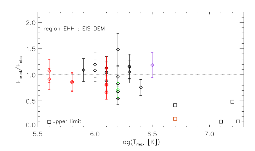
Figure 7.— Top: Emission measure distribution derived for region EHH with the MCMC method (see text) using EIS line fluxes listed in Table 2. The error bars provide a measure of the extent to which the $EM(T)$ of each temperature bin is constrained by the measured fluxes. We plot uncertainties only for the temperature bins for which the $EM(T)$ contributes to at least 5% of the flux of at least one line (see Figure 8, and text for details). Unconstrained bins are plotted with dashed line. Bottom: Comparison of measured EIS line fluxes with flux values predicted using the emission measure distribution derived with the MCMC method. Different colors are used for lines of different elements, in accordance with the colors used to show the EM loci (Figure 6).

We can investigate the compatibility of this derived $EM(T)$ with the XRT observations by computing the predicted XRT fluxes and comparing them with the measured ones. It is worth noting however that when deriving the $EM(T)$ using exclusively the information contained in the EIS spectra, not all temperature bins are well constrained. In particular for these EIS datasets which lack measured lines in the high temperature range ($\log T[{\rm K}]\gtrsim 6.5$) the hot tail of the $EM(T)$ is poorly constrained, but XRT is very sensitive to it, having temperature responses which peak around $\log T[{\rm K}]\sim 7$ for all filters. Therefore some caution must be applied to perform this cross-check. To determine in which temperature bins the $EM(T)$ is constrained by EIS data we look at the contribution of each bin to the line fluxes. Folding the $EM(T)$ with the line emissivity we can investigate the relative weight of each temperature bin for each line, as shown in Figure 8. We then consider as constrained the temperature bins where the $EM(T)$ contributes more than a threshold (percentage) value to at least one of the EIS lines. The choice of the threshold value is somewhat arbitrary and we chose a rather conservative 5%.

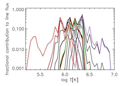
Figure 8.— Each curve represents the fractional contribution of each temperature bin to the flux of one of the EIS lines used for DEM reconstruction (hot lines for which we only derived upper limits are not shown). We use the same colors as in Figure 6.

Considering the $EM(T)$ in the temperature bins satisfying our selection criterium, we calculate the predicted fluxes in the XRT filters (which therefore are strictly speaking lower limits to the values predicted by the assumed $EM(T)$) which are listed in Table 4, together with the measured fluxes. The comparison of the two sets indicates that the $EM(T)$ derived from EIS underpredicts the XRT fluxes by a factor $\sim 2$, the discrepancy being slightly larger for the thinner filters (Al-poly, C-poly, Ti-poly) which are more sensitive to the cooler plasma which is better characterized by the EIS data.

Table 4For region EHH, comparison of XRT measured fluxes with the values predicted using the $EM(T)$ derived from EIS line fluxes (and shown in the upper panel of Figure 7), and from the forward modeling with two temperature components (see §3.2), assuming coronal abundances.

XRT filter	Fobs	Fpred,EIS	Fpred,fm
	[DN/s]	[DN/s]	[DN/s]
Al-poly	122.0	57.8 (41.8-70.2)	123.2
C-poly	95.8	44.5 (32.8-53.4)	101.1
Ti-poly	69.1	31.0 (23.0-36.9)	65.94
Be-thin	11.1	5.85 (3.69-7.61)	9.82
Be-med	1.59	1.06 (0.66-1.38)	1.42
Al-med	0.730	0.483 (0.301-0.628)	0.673

3.2. Thermal Structuring from XRT data

We then derive the thermal distribution of the coronal plasma exclusively from XRT data, by using two different methods:

• Forward fitting of distributions of filter ratios of several filter pairs, through pixel-by-pixel Monte Carlo simulations of the observations, using two temperature components (2T);

• MCMC method, as for the analysis of the EIS spectra (see §3.1).

We use XRT temperature responses calculated assuming “coronal” abundances (Feldman, 1992) and the new XRT calibration which includes a model for the contamination layers deposited both on the CCD and on the focal plane filters (N.Narukage et al., 2010, Solar Physics, submitted). For the detailed comparison of XRT and EIS data for each of the selected region we only use the subset of XRT data taken simultaneously to the EIS observations (see Fig. 3).

We have applied the forward fitting method with two T components already in previous analysis of XRT data aimed at deriving the plasma temperature distribution of an active region, in particular to investigate the presence of a high temperature component (Reale et al., 2009b). The details of this method are thoroughly discussed by Reale et al. (2009b). In summary, the pixel fluxes in the relevant XRT filters are computed from a basic model EM(T) along the line of sight defined by few parameters (amplitude, central temperature, and width of either single or double top-hat functions). Monte Carlo simulations are used to randomize some of the EM(T) parameters and to include Poisson photon noise. This procedure is replicated to build whole fake XRT images in all filters. The simulated XRT data are then analyzed exactly as they were actual data: (1) temperature and emission measure maps, i.e., single values for each pixel, are obtained for a given filter ratio, and this is done for several filter pairs which are sampling the thermal structure in different ways; (2) for each considered filter ratio an emission measure distribution vs. temperature is built by summing up the emission measure values of all pixels falling in the same temperature bin. The input $EM(T)$ is deemed an adequate representation of the underlying plasma emission measure distribution when these curves of emission measure distributions vs. temperature are reproducing satisfactorily the analogous curves obtained from actual data.

Figure 9.— Top: Emission measure distribution vs. temperature derived for region EHH from XRT data. Each curve correspond to a filter pair: soft filter ratios (thin solid lines), Al_med/Be_thin (dotted line), Be_med/Be_thin (dashed line), Be_med/Al_med (thick solid line). Bottom: Emission measure distribution vs. temperature derived for region EHH from XRT data simulated using the $EM(T)$ histogram as parent emission measure distribution along the line of sight. Lines as in the top panel.

The results of these simulations for region EHH are shown in Figure 9, and Table 4. We note that, as discussed thoroughly in Reale et al. (2009b) for the analysis of XRT observations of another active region, while this analysis method is certainly approximate it allows us to be sensitive to possible minor EM(T) components, e.g., small hot components, and to somewhat constrain them. As for the case presented in Reale et al. (2009b), also here we find that a high temperature plasma component, even if much weaker than the dominating cool ($\log T[{\rm K}]\sim 6.1-6.3$), is nevertheless appropriate to reproduce the XRT observations.

As mentioned above, in order to derive the $EM(T)$ from XRT data we also use the MCMC method, using the flux values integrated in each passband over the whole subregion. The errors associated to the XRT fluxes are estimated by taking into account the photon noise and the calibration uncertainties. Like for the EIS fluxes, the statistical uncertainties (we observe bright sources and integrate over time to further increase the signal-to-noise ratio) are typically very small and the errors are largely dominated by the calibration uncertainties (for an estimate of the latter see Narukage et al. 2010, Solar Physics, submitted). The resulting errors are of the order of $\sim 5$% for the thin filters, and $\sim 15-20$% for thin-Be and the medium filters. The derived best fit $EM(T)$ is shown in Figure 10 (red line); the associated uncertainties are rather large, as should also be expected considering the limited constraints that the XRT fluxes in six filters can provide to the emission measure distribution over a large temperature range.

The differences between the results of the two methods are not large, compared to the associated uncertainties. The agreement is overall acceptable if one considers that the approaches are completely different. The MCMC method is model independent but it only uses the total region flux values. The forward fitting 2T method makes an assumption on the basic EM(T) distribution but it keeps the spatial information of the pixel values longer in the analysis pipeline, and it is therefore more sensitive to small local plasma inhomogeneities (at the scale of the single pixel). Moreover this latter method gives large weight to the Be_med/Al_med filter ratio, and this allows to detect the small hot component.

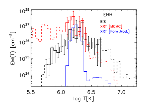
Figure 10.— Comparison of emission measure distribution derived for region EHH independently from EIS lines (with MCMC method, see §3.1; black line), and from XRT, with two different methods: MCMC (red line), and forward modeling with two temperature components (blue line). For the $EM(T)$ derived using the MCMC method we show the estimate of uncertainties for those temperature bins which contribute to at least 5% to the flux of at least one line or passband (see Figure 8).

In Figure 10 we compare the emission measure distributions derived independently from XRT and EIS data. Considering only the temperature regions where the EM(T) are constrained by the data, i.e. the bins where the error bars are shown, the different datasets yield emission measure distributions that are not too dissimilar when the (large) uncertainties are taken into account. In particular, they have similar peak temperature and width of the cool component. Using the $EM(T)$ derived from XRT data with the MCMC method to calculate the expected fluxes for the EIS lines of Table 2, we find that the XRT $EM(T)$ reproduces the measured EIS fluxes not too accurately. Specifically, the lines with typical temperature of formation $\log T[{\rm K}]\gtrsim 6.3$, such as Fe xiv and Fe xv, and the lines formed around $\log T[{\rm K}]\sim 6.1-6.2$, such as Fe xii and Si x, are overpredicted by a factor $\sim 3$ (typical range spans approximately from a factor 2 to 5); cooler lines ($\log T[{\rm K}]\lesssim 6.0$) are instead slightly underpredicted (typical range: $\sim 0.05$ to $\sim 1.5\times$ the measured fluxes).

3.3. Thermal Structuring from EIS and XRT 

We finally take advantage of all the available information, and derive the plasma $EM(T)$ by applying the MCMC method to the measured XRT and EIS fluxes together. The $EM(T)$ derived for region EHH by combining the two instruments is shown in Figure 11, compared to the emission measure distributions derived independently from each of the two datasets.

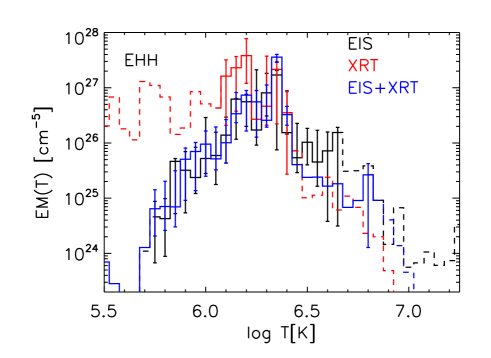
Figure 11.— Comparison of emission measure distribution derived for region EHH with different methods: from EIS lines (black line; same curve as Figure 10), from XRT (red line; same curve as curve shown in Figure 10), and using EIS and XRT data together (blue curve).

When combining XRT and EIS data, the resulting $EM(T)$ is overall rather similar to the $EM(T)$ derived from EIS data, which provide much tighter constraints because of the large number of lines, and temperature dependence of their emissivity. In the high temperature range however, where XRT is more sensitive to the plasma emission and EIS provides poor constraints, the XRT+EIS $EM(T)$ departs more from the EIS curve.

Figure 12 shows how well the XRT+EIS $EM(T)$ reproduces the measured fluxes. While the EIS line fluxes are reproduced reasonably well, similarly to the case of the EIS $EM(T)$, there is some systematic discrepancy between the predicted and the observed fluxes in the XRT  passbands. Specifically, the three cooler filters, Al-poly, C-poly, Ti-poly, are underpredicted by about a factor 2. The fluxes in the hotter filters are instead well reproduced. We note that for these latter filters, which are much less sensitive to cool plasma with respect to the thin filters, the algorithm of derivation of the emission measure distribution can find a satisfactory agreement with the observations because of the leeway in the determination of the high temperature component which is not tightly constrained by the other fluxes, and in particular does not contribute significantly to the analyzed EIS lines. These discrepancies are reminiscent of the systematics found when predicting XRT fluxes using the EIS $EM(T)$ (see Table 4), and when using the XRT $EM(T)$ to predict the EIS line fluxes (see discussion at end of §3.2). The cross-check provided by the three methods points to a systematic difference with EIS data yielding emission measure values a factor $\sim 2$ lower than the values derived from XRT data, as also evident from Figure 11.

We explored how some of the assumptions we have made for our analysis may affect these results. Among those, the assumption for the element abundances of the coronal plasma has a potentially very significant effect on the derivation of the plasma emission measure distribution. There is a large body of evidence that element abundances in the solar corona do not reflect the solar photospheric composition (e.g., Meyer, 1985; Feldman, 1992). In particular, the chemical fractionation appears to be a function of the First Ionization Potential (FIP), with low FIP elements, such as Fe and Si, typically enhanced in the corona by a factor of a few, whereas high FIP elements such as O are thought to have coronal abundances close to their photospheric values (e.g., Meyer, 1985; Feldman, 1992).

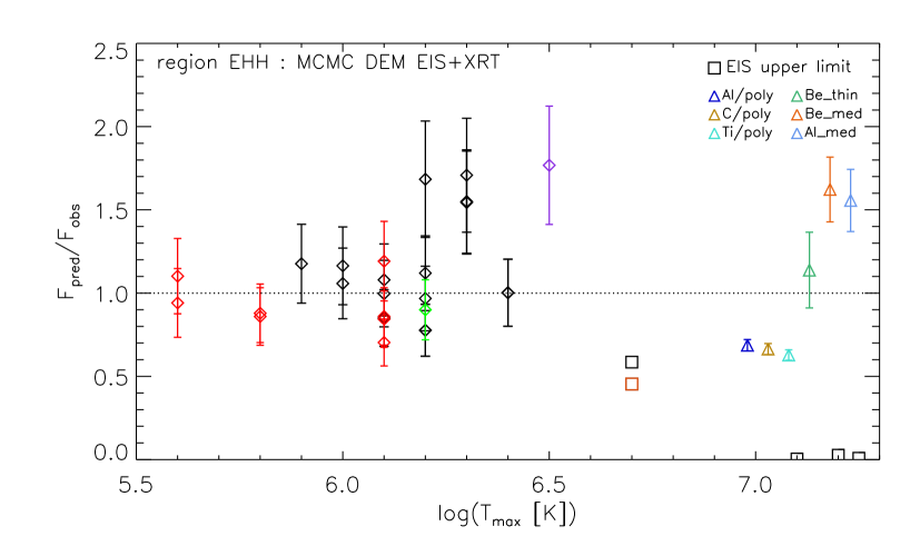
Figure 12.— Comparison of measured EIS and XRT fluxes with flux values predicted using the emission measure distribution derived with the MCMC method using both set of fluxes and shown in Figure 11. We use the same colors as in Figure 6 to indicate lines of different elements or XRT passbands.

The intensity of spectral lines is linearly dependent on the element abundance (assuming that the abundance is the same at all temperatures for plasma in the studied region; see Eq. 1). Therefore, if the $EM(T)$ is derived from lines all emitted from a single element, e.g. Fe, a change in the element abundance will not change the shape of the emission measure distribution but merely shift its absolute value: for instance, a decrease of the abundance by a factor 2 will determine an increase of the $EM(T)$ by a factor 2. Although our analysis of EIS data includes lines emitted by different elements, the large majority of the considered lines are emitted by low FIP elements Fe and Si. Therefore, if we consider a chemical composition with a FIP bias different from the Feldman (1992) set, typically adopted for coronal plasma and used for all the above analysis, we expect the shape of the $EM(T)$ to not change by much qualitatively even its absolute values can change significantly.

For wide band instruments like XRT the effect the adopted chemical composition of the plasma on the temperature response is not as straightforward, as at different temperatures the relative contribution of the emission from different elements can change significantly. In Figure 13 we show the effect of the element abundances on the temperature response of the XRT filters used in this work. We consider the Feldman (1992) “coronal” abundances, and a set of abundances intermediate between coronal and photospheric Grevesse & Sauval (1998), i.e. with a FIP bias of 2 instead of 4 which is typically assumed for coronal plasma. For instance for this set of abundances Fe, Si and Mg have abundances about half the values of Feldman (1992).

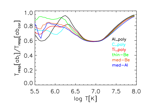
Figure 13.— Ratio of XRT responses, as a function of temperature, calculated using intermediate abundances (FIP bias = 2), to the responses calculated using coronal abundances (Feldman, 1992). A different color is used for each filter used in this work, as indicated in the inset.

Figure 13 shows that in the range $\log T[{\rm K}]\sim 6.7-7.3$ the change in the responses is approximately linear with the abundances of these low FIP elements which are dominating the emission in this high temperature range. At lower temperatures however the XRT filters are affected differently depending on the details of their response as a function of wavelength and therefore the importance of different lines.

We repeated our analysis using different sets of abundances, and in particular we derived the $EM(T)$ using this set of intermediate abundances described here above, and the set of photospheric abundances of Grevesse & Sauval (1998). The results we obtained are shown in Figure 14, also compared to the $EM(T)$ derived with Feldman abundances. The curves have very similar shape and are overall compatible within the uncertainties. However it is clear that, as expected in the light of the above discussions, the $EM(T)$ obtained for intermediate abundances (which are lower than the “coronal” abundances) is systematically larger than the one found for “coronal” abundances, and the $EM(T)$ derived for the photospheric abundances case are even larger. In the middle panel of Figure 14 we show the comparison of the observed fluxes with the predictions using the $EM(T)$ derived for intermediate abundances. Comparing these findings with the analogous results of Figure 12 we note that although the overall results are not changed dramatically, the fluxes predicted for the XRT thin filters are closer to the observations when using intermediate abundances. The increases by about 20-35% are compatible with expectations: the predicted fluxes should rise accordingly to the increase of the cool component of the $EM(T)$  but be reduced by a factor corresponding to the decrease of the XRT response (see Figure 13). The analogous plot for the case of photospheric abundances (bottom panel of Figure 14) shows that using these abundance values the agreement between EIS and XRT improves even further.

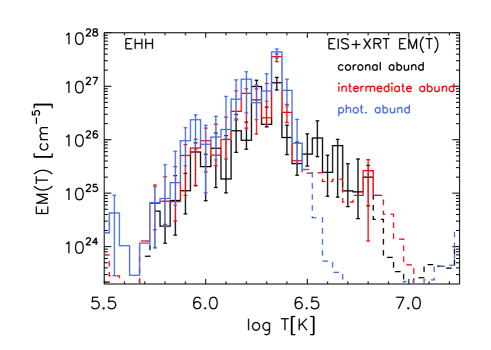
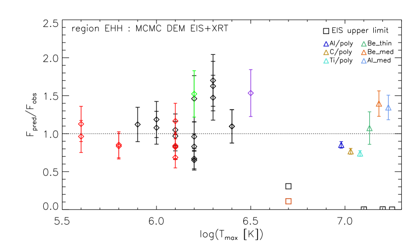
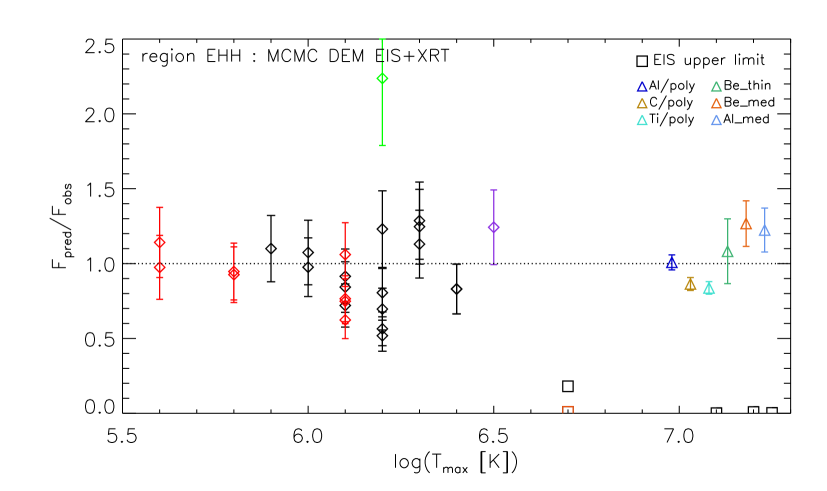
Figure 14.— Top panel: Comparison of emission measure distributions derived with the MCMC method using simultaneously EIS and XRT fluxes, and three different sets of abundances: coronal abundances (Feldman 1992; black line), intermediate abundances (red line; see text for definition of intermediate abundances), and photospheric abundances (Grevesse & Sauval 1998; blue line). For intermediate abundances, for which Fe and Si have roughly half the abundance as in the coronal set, the $EM(T)$ accordingly increases; the $EM(T)$ increases even further for photospheric abundances. Middle and bottom panels: Comparison of measured EIS and XRT fluxes with flux values predicted by the emission measure distribution derived with the MCMC method (XRT+EIS) and: (a) intermediate abundances (middle), or (b) photospheric abundances (bottom; Grevesse & Sauval 1998).

The values assumed for the element abundances can in principle be checked with the EIS spectra. As discussed above, the DEM obtained from EIS has been determined using almost exclusively lines from low-FIP ions, whose coronal abundances are enhanced by a factor of $\sim 3-4$ over the photospheric values. Therefore, any change in the actual abundance of the low-FIP elements from the assumed value will result in a systematic shift between the observed intensities of the lines from S x to S xiii, whose coronal abundance is expected to be close to the photospheric one, and their values predicted with the DEM. There are ten S lines in the EIS spectra, emitted by S x to S xiii, and we have compared their predicted and observed intensities to check the corrections to the coronal abundances. We found no unambiguous evidence of systematic differences in the observed to predicted intensity ratios. Moreover, recent estimates of the S absolute abundance have been revised by Lodders (2003) and by Caffau & Ludwig (2007), who decreased them by a factor 1.5 from the Grevesse & Sauval (1998) value. Since this change is of the same order of the revision of the low-FIP element abundances we propose, we feel that the uncertainties in the S predicted line intensities are so large that these ions can not be used to confirm the abundance change made necessary by the XRT channels in this work. S is in any case a borderline element for FIP effect studies, and abundances of other low FIP elements are difficult to determine. While oxygen lines of O iv,v,vi are present in the EIS wavelength range, they are formed at low temperature ($\log(T[K])\lesssim 5.5$) with respect to the hotter coronal EIS lines considered in our active region study. In that temperature range the thermal distribution is not well constrained and therefore the abundances cannot be accurately determined.

While the results shown in Figure 14 seem to suggest that the photospheric abundances might be a more appropriate choice for the active region we studied here, we note that the data we have used do not allow us to determine the abundances and therefore do not allow us to disentangle between the abundance effects and cross-calibration issues. We also note that this active region was already several days old at the time of the observation, and therefore it is reasonable to expect some significant effect of chemical fractionation to have occurred producing departures from the photospheric composition (see e.g., Widing & Feldman 2001; however, see also Del Zanna 2003).

We have presented the complete analysis carried out for one of the selected regions, providing insights into the thermal distribution of the plasma, limitations of the methods, and cross-calibration of the Hinode XRT and EIS. Before discussing in details these findings in §4 we briefly present and discuss the analogous results found for the other two selected regions, EC and EH, comparing them with the results obtained for region EHH.

Carrying out the same analysis described above (§3.1, 3.2, 3.3) on the other two regions, we find results qualitatively similar to our findings for region EHH discussed above, in particular in terms of the comparison between different analysis methods and systematic discrepancies between XRT and EIS.

In Figure 15 we show the emission measure distributions obtained for the three regions, using the MCMC algorithm applied to XRT and EIS data together (top panel), or forward fitting the XRT observations using two temperature components (bottom panel). We note that despite the forward fitting 2T model adopts considerable simplifying assumptions for the underlying emission measure distribution the results we obtain with this method are qualitatively in good agreement with the MCMC approach which does not impose constraints on the shape of the DEM. On the other hand, we note that the forward fitting 2T model has the advantage of also taking into account the spatial information, while the MCMC method only uses the information contained in the integrated fluxes in each passband. The two hotter regions, EH and EHH, have very similar underlying $EM(T)$: their cool components have analogous peak temperature ($\log T[{\rm K}]\sim 6.2-6.3$) and amounts of plasma, whereas the hot component of EHH is of weight comparable to the high temperature component of EH but it appears shifted towards slightly higher temperatures. For region EC the cool component is characterized by a peak temperature slightly cooler than the other two regions, and in particular its $EM(T)$ falls off faster on the high temperature side of the cool peak; the hot component of EC is much weaker than the other two components, if at all present.

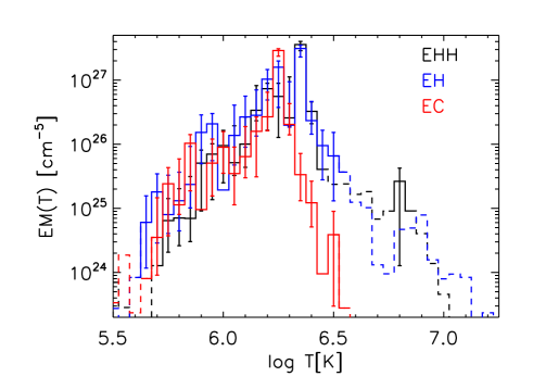
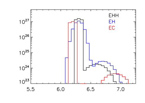
Figure 15.— Emission measure distributions for the three selected regions: EC (red line), EH (blue line), EHH (black line). Top: $EM(T)$ curves derived with MCMC method, using EIS and XRT fluxes. Bottom: $EM(T)$ derived from XRT data through the forward fitting 2T method (see §3.2 for details), using photospheric abundances.

4. Discussion

We have presented the results of a detailed analysis of Hinode XRT and EIS observations of a non-flaring active region to diagnose the temperature distribution of the coronal plasma. In this work we carried out independent temperature analysis from measurements of either instruments, and use the derived thermal distributions to make prediction for the fluxes observed with the other instrument and then compare them with actual measurements. Then we combine the information from both instruments and compare the results with the findings based on XRT or EIS data only. This approach allowed us to explore the limitations of the data and analysis methods in providing constraints to the plasma temperature distribution, and investigate the cross-calibration of the two Hinode instruments. With respect to previous works using both XRT and EIS data to study the thermal properties of the coronal plasma (e.g., Landi et al., 2010), in this work we provide a quantitative cross-check between the diagnostics of the two instruments.

When using the two datasets separately the derived $EM(T)$ curves have overall similar width and peak temperature. However, the emission measure derived from EIS is systematically smaller, by a factor $\sim 2-3$, than the emission measure derived from XRT fluxes, for each of the three studied regions. We note that even if the uncertainties in the derived $EM(T)$ are rather large the systematic discrepancy appears to be significant. We find that the extent of the discrepancy between XRT and EIS depends in part on the assumptions made for the chemical composition of the X-ray emitting plasma: it can be mitigated by assuming abundances intermediate between the typical “coronal” abundances (Feldman, 1992) and the photospheric values Grevesse & Sauval (1998), and it almost disappears when using photospheric abundances. This interesting finding encourages further investigations to search for similar evidence in other active regions, in an active region at different epochs, and in different kinds of coronal structures (quiet sun, bright points, coronal holes). While our study provides no robust constraints on the element abundances we stress the importance of the assumed values in the analysis of Hinode observations. The detailed $EM(T)$ reconstruction and the instrument cross-calibration are significantly affected by the assumed abundances: EIS spectra allow the determination of “abundance independent” $EM(T)$  e.g. using exclusively Fe lines (Watanabe et al., 2007), but its absolute values depend on the abundances; the XRT passbands include significant contribution of several elements, both high-FIP and low-FIP, and therefore the dependence of the $EM(T)$ on abundances is more complicated and temperature dependent.

For the analysis of XRT data we use two different methods for deriving the emission measure distribution. We find that the Markov-chain Monte Carlo method yields results in good qualitative agreement with the forward fitting 2T method which makes rather simplifying assumptions on the emission measure distribution but has the advantage of making use also of the spatial information. This finding lends further confidence to the results obtained previously by applying this method to the study of XRT observations of another active region (Reale et al., 2009b).

We find that the EIS spectra allow an accurate determination of the cool ($\log T[$K$]\lesssim 6.5$), most prominent, component, but when used alone the EIS data are unable to constrain the hotter emission due to the lack of strong hot lines in the spectra. The combination with XRT data provide much tighter constraints on the emission measure distribution on a wider temperature range. Our analysis shows that the studied active region is characterized by bulk plasma temperatures of $\sim 2$ MK, which are rather low for active region plasma. The $EM(T)$ of the three selected regions are very similar for $\log T[$K$]\lesssim 6.2$, but for the two hotter regions, EH and EHH, the cool component is broader and with a peak shifted towards higher T. The high temperature tail of the emission measure distribution is not strongly constrained by the data. However, the $EM(T)$ derived at least for the two hotter regions, EH and EHH, suggests the presence of a hotter component ($\log T[{\rm K}]\gtrsim 6.5$) about two orders of magnitude weaker than the dominant cool component, in good agreement with the findings of Reale et al. (2009b) for another, hotter, active region.

5. Conclusions

We analyzed Hinode XRT multi-filter data and EIS spectral observations of a non-flaring active region to study the temperature distribution of coronal plasma, $EM(T)$, and to carry out a detailed investigation of the cross-calibration of the two instruments. We selected three subareas of the active region, and for each of them we derived the emission measure distribution $EM(T)$ by: (1) using EIS measured line fluxes; (2) using XRT fluxes in six of the instrument’s filters; (3) combining the datasets for the two instruments.

We find a good consistency in the qualitative characteristics – peak temperature and width of dominant temperature component– of the $EM(T)$ derived with different methods. However, the emission measure distributions derived by the two instruments XRT and EIS indicate a systematic discrepancy between the two instruments, with EIS data yielding $EM(T)$ consistently smaller, by about a factor 2, than the $EM(T)$ compatible with XRT data. We discuss the possible origin of the disagreement and find that the assumptions for the element abundances significantly influence the plasma temperature diagnostics. In particular we find that a chemical composition intermediate between the usually adopted coronal abundances by Feldman (1992) and the solar photospheric abundances improves the comparison between the results obtained with the two instruments. When adopting photospheric abundances the discrepancy between EIS and XRT decreases further. However we note that it seems unlikely that the observed plasma, in an active region which is not newly emerged, has photospheric composition. Furthermore, the used data do not allow a definite determination of the abundances, and therefore do not allow us to robustly assess of the cross-calibration of the instruments.

One of the main aims of this work was to exploit the complementary diagnostics for the X-ray emitting plasma provided by XRT and EIS, to investigate the presence of hot plasma in non-flaring regions and test nanoflare heating models. We find that the derived $EM(T)$ are characterized by an expected dominant cool component (typically $\log T[{\rm K}]\sim 6.3$), and a much weaker amount of plasma at higher temperature. While the amount of hot plasma is in general in agreement with recent findings for other non-flaring active regions, and it is compatible with expectations from nanoflare models, we find that within the uncertainties these results are not conclusive.

References

- Aschwanden et al. (2000) Aschwanden, M. J., Nightingale, R. W., & Alexander, D. 2000, ApJ, 541, 1059
- Brooks et al. (2009) Brooks, D. H., Warren, H. P., Williams, D. R., & Watanabe, T. 2009, ApJ, 705, 1522
- Brosius et al. (1996) Brosius, J. W., Davila, J. M., Thomas, R. J., & Monsignori-Fossi, B. C. 1996, ApJS, 106, 143
- Bryans et al. (2009) Bryans, P., Landi, E., & Savin, D. W. 2009, ApJ, 691, 1540
- Caffau & Ludwig (2007) Caffau, E., & Ludwig, H. 2007, A&A, 467, L11
- Cargill (1994) Cargill, P. J. 1994, ApJ, 422, 381
- Cargill & Klimchuk (1997) Cargill, P. J., & Klimchuk, J. A. 1997, ApJ, 478, 799
- Craig & Brown (1976) Craig, I. J. D., & Brown, J. C. 1976, A&A, 49, 239
- Culhane et al. (2007) Culhane, J. L., Harra, L. K., James, A. M., Al-Janabi, K., Bradley, L. J., Chaudry, R. A., Rees, K., Tandy, J. A., Thomas, P., Whillock, M. C. R., Winter, B., Doschek, G. A., Korendyke, C. M., Brown, C. M., Myers, S., Mariska, J., Seely, J., Lang, J., Kent, B. J., Shaughnessy, B. M., Young, P. R., Simnett, G. M., Castelli, C. M., Mahmoud, S., Mapson-Menard, H., Probyn, B. J., Thomas, R. J., Davila, J., Dere, K., Windt, D., Shea, J., Hagood, R., Moye, R., Hara, H., Watanabe, T., Matsuzaki, K., Kosugi, T., Hansteen, V., & Wikstol, Ø. 2007, Sol. Phys., 243, 19
- Del Zanna (2003) Del Zanna, G. 2003, A&A, 406, L5
- Del Zanna & Mason (2003) Del Zanna, G., & Mason, H. E. 2003, A&A, 406, 1089
- Dere et al. (1997) Dere, K. P., Landi, E., Mason, H. E., Monsignori Fossi, B. C., & Young, P. R. 1997, A&AS, 125, 149
- Dere et al. (2009) Dere, K. P., Landi, E., Young, P. R., Del Zanna, G., Landini, M., & Mason, H. E. 2009, A&A, 498, 915
- Doschek et al. (2007) Doschek, G. A., Mariska, J. T., Warren, H. P., Culhane, L., Watanabe, T., Young, P. R., Mason, H. E., & Dere, K. P. 2007, PASJ, 59, 707
- Feldman (1992) Feldman, U. 1992, Phys. Scr, 46, 202
- Golub et al. (2007) Golub, L., Deluca, E., Austin, G., Bookbinder, J., Caldwell, D., Cheimets, P., Cirtain, J., Cosmo, M., Reid, P., Sette, A., Weber, M., Sakao, T., Kano, R., Shibasaki, K., Hara, H., Tsuneta, S., Kumagai, K., Tamura, T., Shimojo, M., McCracken, J., Carpenter, J., Haight, H., Siler, R., Wright, E., Tucker, J., Rutledge, H., Barbera, M., Peres, G., & Varisco, S. 2007, Sol. Phys., 243, 63
- Grevesse & Sauval (1998) Grevesse, N., & Sauval, A. J. 1998, Space Science Reviews, 85, 161
- Judge (2010) Judge, P. G. 2010, ApJ, 708, 1238
- Judge et al. (1997) Judge, P. G., Hubeny, V., & Brown, J. C. 1997, ApJ, 475, 275
- Kashyap & Drake (1998) Kashyap, V., & Drake, J. J. 1998, ApJ, 503, 450
- Kashyap & Drake (2000) —. 2000, Bulletin of the Astronomical Society of India, 28, 475
- Klimchuk (2006) Klimchuk, J. A. 2006, Sol. Phys., 234, 41
- Kosugi et al. (2007) Kosugi, T., Matsuzaki, K., Sakao, T., Shimizu, T., Sone, Y., Tachikawa, S., Hashimoto, T., Minesugi, K., Ohnishi, A., Yamada, T., Tsuneta, S., Hara, H., Ichimoto, K., Suematsu, Y., Shimojo, M., Watanabe, T., Shimada, S., Davis, J. M., Hill, L. D., Owens, J. K., Title, A. M., Culhane, J. L., Harra, L. K., Doschek, G. A., & Golub, L. 2007, Sol. Phys., 243, 3
- Landi et al. (2002) Landi, E., Feldman, U., & Dere, K. P. 2002, ApJS, 139, 281
- Landi & Landini (1998) Landi, E., & Landini, M. 1998, A&A, 340, 265
- Landi et al. (2009) Landi, E., Miralles, M. P., Curdt, W., & Hara, H. 2009, ApJ, 695, 221
- Landi et al. (2010) Landi, E., Raymond, J. C., Miralles, M. P., & Hara, H. 2010, ApJ, 711, 75
- Lang et al. (2006) Lang, J., Kent, B. J., Paustian, W., Brown, C. M., Keyser, C., Anderson, M. R., Case, G. C. R., Chaudry, R. A., James, A. M., Korendyke, C. M., Pike, C. D., Probyn, B. J., Rippington, D. J., Seely, J. F., Tandy, J. A., & Whillock, M. C. R. 2006, Appl. Opt., 45, 8689
- Lodders (2003) Lodders, K. 2003, ApJ, 591, 1220
- McTiernan (2009) McTiernan, J. M. 2009, ApJ, 697, 94
- Meyer (1985) Meyer, J. 1985, ApJS, 57, 173
- O’Dwyer et al. (2010) O’Dwyer, B., Del Zanna, G., Mason, H. E., Sterling, A. C., Tripathi, D., & Young, P. R. 2010, A&A, in press
- Parenti et al. (2006) Parenti, S., Buchlin, E., Cargill, P. J., Galtier, S., & Vial, J. 2006, ApJ, 651, 1219
- Parker (1972) Parker, E. N. 1972, ApJ, 174, 499
- Parker (1988) —. 1988, ApJ, 330, 474
- Patsourakos & Klimchuk (2009) Patsourakos, S., & Klimchuk, J. A. 2009, ApJ, 696, 760
- Reale et al. (2009a) Reale, F., McTiernan, J. M., & Testa, P. 2009a, ApJ, 704, L58
- Reale et al. (2007) Reale, F., Parenti, S., Reeves, K. K., Weber, M., Bobra, M. G., Barbera, M., Kano, R., Narukage, N., Shimojo, M., Sakao, T., Peres, G., & Golub, L. 2007, Science, 318, 1582
- Reale et al. (2009b) Reale, F., Testa, P., Klimchuk, J. A., & Parenti, S. 2009b, ApJ, 698, 756
- Schmelz et al. (2009a) Schmelz, J. T., Kashyap, V. L., Saar, S. H., Dennis, B. R., Grigis, P. C., Lin, L., De Luca, E. E., Holman, G. D., Golub, L., & Weber, M. A. 2009a, ApJ, 704, 863
- Schmelz et al. (2009b) Schmelz, J. T., Saar, S. H., DeLuca, E. E., Golub, L., Kashyap, V. L., Weber, M. A., & Klimchuk, J. A. 2009b, ApJ, 693, L131
- Shestov et al. (2010) Shestov, S. V., Kuzin, S. V., Urnov, A. M., Ul’Yanov, A. S., & Bogachev, S. A. 2010, Astronomy Letters, 36, 44
- Sylwester et al. (2010) Sylwester, B., Sylwester, J., & Phillips, K. J. H. 2010, A&A, 514, A82+
- Testa et al. (2002) Testa, P., Peres, G., Reale, F., & Orlando, S. 2002, ApJ, 580, 1159
- Tripathi et al. (2010) Tripathi, D., Mason, H. E., Del Zanna, G., & Young, P. R. 2010, A&A, 518, A42+
- Warren & Brooks (2009) Warren, H. P., & Brooks, D. H. 2009, ApJ, 700, 762
- Warren et al. (2010) Warren, H. P., Kim, D. M., DeGiorgi, A. M., & Ugarte-Urra, I. 2010, ApJ, 713, 1095
- Warren et al. (2008) Warren, H. P., Ugarte-Urra, I., Doschek, G. A., Brooks, D. H., & Williams, D. R. 2008, ApJ, 686, L131
- Warren et al. (2003) Warren, H. P., Winebarger, A. R., & Mariska, J. T. 2003, ApJ, 593, 1174
- Watanabe et al. (2007) Watanabe, T., Hara, H., Culhane, L., Harra, L. K., Doschek, G. A., Mariska, J. T., & Young, P. R. 2007, PASJ, 59, 669
- Watanabe et al. (2009) Watanabe, T., Hara, H., Yamamoto, N., Kato, D., Sakaue, H. A., Murakami, I., Kato, T., Nakamura, N., & Young, P. R. 2009, ApJ, 692, 1294
- Widing & Feldman (2001) Widing, K. G., & Feldman, U. 2001, ApJ, 555, 426
- Young et al. (2007) Young, P. R., Del Zanna, G., Mason, H. E., Dere, K. P., Landi, E., Landini, M., Doschek, G. A., Brown, C. M., Culhane, L., Harra, L. K., Watanabe, T., & Hara, H. 2007, PASJ, 59, 857
- Young et al. (1998) Young, P. R., Landi, E., & Thomas, R. J. 1998, A&A, 329, 291
- Young et al. (2009) Young, P. R., Watanabe, T., Hara, H., & Mariska, J. T. 2009, A&A, 495, 587