Death of soliton trains in attractive Bose-Einstein condensates

Abstract

Experiments on ultra-cold attractive Bose-Einstein Condensates (BECs) have demonstrated that at low dimensions atomic clouds can form localized objects, propagating for long times without significant changes in their shapes and attributed to bright matter-wave solitons, which are coherent objects. We consider the dynamics of bright soliton trains from the perspective of many-boson physics. The fate of matter-wave soliton trains is actually to quickly loose their coherence and become macroscopically fragmented BECs. The death of the coherent matter-wave soliton trains gives birth to fragmented objects, whose quantum properties and experimental signatures differ substantially from what is currently assumed.

Solitons are common wave-packet phenomena in many areas of science and engineering sol1 ; sol2 . Such localized structures can form when a wave-packet’s dispersion is compensated by self-focusing (attractive) forces. In this context, the physics of low-dimensional attractive Bose-Einstein condensates (BECs) has attracted much attention solth1 ; solth2 ; exp1 ; exp2 ; attrac1 ; attrac2 ; attrac3 ; attrac4 . The similarity between the Gross-Pitaevskii (GP) equation GP1 ; GP2 commonly used to describe these ultra-cold quantum systems and the non-linear Schrödinger equation used in optics sol2 to characterize self-focusing of light has encouraged the transfer of ideas, phenomena, and understanding from optics to ultra-cold atomic physics. Particularly, bright matter-wave solitons have been predicted to occur in low-dimensional attractive Bose gases solth1 ; solth2 , stimulating the recent experiments exp1 ; exp2 .

Very often, along with a single soliton, multi-hump matter-wave structures propagating for long times without significant changes in their shapes have been observed. Since the GP equation supports localized multi-hump solutions as excited states, the experimentally observed multi-hump structures have been attributed to soliton trains, which are coherent objects. This is the current widely accepted interpretation in the literature. Nowadays the GP equation (i.e., the non-linear Schrödinger equation) is the cornerstone of studying soliton trains in attractive BECs.

It is important to remember, however, that ultra-cold attractive BECs are quantum many-particle systems, governed by the many-boson Schrödinger equation. Hence, we consider in this work the dynamics of bright soliton trains from the perspective of many-boson physics. As we shall show the fate of matter-wave soliton trains is to quickly loose their coherence and become macroscopically fragmented BECs frag1 ; frag2 ; frag3 . The death of the coherent matter-wave soliton trains gives birth to fragmented objects, whose quantum properties and experimental signatures differ substantially from what is currently assumed.

Our starting point is the GP dynamics $\left[-\frac{1}{2}\frac{\partial^{2}}{\partial x^{2}}+\lambda_{0}(N-1)|\psi(x,t)|^{2}\right]\psi(x,t)=i\frac{\partial\psi(x,t)}{\partial t}$ of a soliton train with two humps (briefly, two-hump soliton). We consider in this work $N=2000$ bosons in one dimension and attractive inter-particle interaction of strength $\lambda_{0}=-0.002$. For convenience, we use dimensionless quantities which are readily arrived at by dividing the dimension-full Hamiltonian by $\frac{\hbar^{2}}{mL^{2}}$, where $m$ is the mass of a boson and $L$ is a length scale. The corresponding dimension-full quantities are within range of current experimental setups and discussed below. As an initial profile (shape) of the two-hump soliton we take the commonly used linear combination of sech-shaped functions:

$$\psi(x,0)={\cal N}\left\{\mathrm{sech}[\gamma(x-x_{0})]\pm\mathrm{sech}[\gamma(x+x_{0})]\right\},$$

where $\cal N$ is the normalization factor. The ”+” refers to a $0$-phase symmetric and the ”-” to a $\pi$-phase anti-symmetric soliton train. The parameter $\gamma$ is inversely proportional to the width of the humps. By assuming a large separation between humps, one gets by minimizing the GP energy functional the optimal value of $\gamma=|\lambda_{0}|(N-1)/4\approx 1.0$.

The time-dependent density $\rho(x,t)$ obtained by solving the time-dependent GP equation for different two-hump solitons is plotted in Fig. 1. In the left upper panel, Fig. 1a, we plot the dynamics for the $0$-phase symmetric soliton train, initially located at $x_{0}=\pm 4.0$. The system reveals the well known mean-field oscillatory dynamics: the humps attract each other, collide at $t\approx 42$, then split and return to the initial separation and start a new cycle of oscillation. The left middle part, Fig. 1b, shows the dynamics for the $\pi$-phase anti-symmetric soliton clouds placed initially at a larger separation of $x_{0}=\pm 6.0$. At such a separation the clouds very slightly repel each other, indicating that the inter-hump forces strongly depend on the initial separation. In the left lower panel, Fig. 1c, we depict the dynamics for a $0$-phase asymmetric soliton train, formed as the combination of the sech-shaped functions of slightly different widths $\gamma=1.1$ (left cloud) and $\gamma=0.9$ (right cloud), placed at $x_{0}=\pm 4.0$. A similar dynamics to Fig. 1a is seen. The GP theory describes the following characteristics of two-hump solitons: (i) the relative phase between humps defines whether the inter-hump interaction is attractive or repulsive, and (ii) the magnitude of the inter-hump interaction depends on the separation between the humps.

We remind the reader that GP theory is a mean-field approximation to the quantum many-boson problem which assumes all bosons to occupy one and the same quantum state throughout the system’s evolution in time. What happens if we relax the constraint of the attractive system to occupy a single quantum state? In other words, we allow the system to choose according to the variational principle its evolution in time by solving now the time-dependent many-boson Schrödinger equation $i\frac{\partial\Psi(t)}{\partial t}=\hat{H}\Psi(t)$, with $\hat{H}(x_{1},\ldots,x_{N})=\sum_{j=1}^{N}-\frac{1}{2}\frac{\partial^{2}}{\partial x_{j}^{2}}+\sum_{j<k}^{N}\lambda_{0}\delta(x_{j}-x_{k})$. It is possible nowadays to go significantly beyond mean-field and compute the dynamics of BECs on the many-body level, by solving the time-dependent many-boson Schrödinger equation with the multiconfigurational time-dependent Hartree method for bosons, see the literature for details MCTDHB_lett ; MCTDHB_pap and applications Grond ; BJJ_us . Is the dynamics of soliton trains described above to change in a dramatic manner?

We take as initial conditions the same $0$-phase symmetric and $\pi$-phase anti-symmetric soliton trains as in the above GP studies and propagate them now not on the mean-field but on the many-body level. The time-dependent density $\rho(x,t)$ obtained at the many-body level is plotted in the right panels of Fig. 1. The first observation is that the initially-localized wave-packets remain localized at the many-body level of the description as well. Hence, localization is indeed a characteristic dynamical feature of attractive bosonic clouds in one dimension, as predicted at the GP level and confirmed here at the many-body level. The many-body results, however, reveal different dynamics than the mean-field ones, compare the left and right panels of Fig. 1. In the right upper panel, Fig. 1d, we depict the many-body dynamics of the initially-prepared $0$-phase symmetric wave-packet. The two separated humps start to attract each other, similarly to the mean-field dynamics, but do not come close enough to collide, as it is in the GP case, Fig. 1a. Instead of the full collision the sub-clouds reach a minimal separation and then they start to depart from each other. This observation reveals, thereby, a repulsive character of the inter-hump interaction. So, during the many-body dynamics the interaction between the humps of the initially-prepared $0$-phase symmetric wave-packet changes from attractive to repulsive and stays repulsive afterwards.

The many-body dynamics of the initially-prepared $\pi$-phase anti-symmetric wave-packet is shown on the right middle panel, Fig. 1e. Due to the larger separation between the two humps, the spatial density profiles obtained at the many-body and GP levels are indeed very close to each other. The weak repulsive interaction between the humps persists at the many-body level as well. The right lower panel, Fig. 1f, shows the density profile for the $0$-phase asymmetric wave-packet constructed, as above, from two functions of slightly different widths. The dynamics obtained at the many-body level for the initially-prepared $0$-phase asymmetric wave-packet has a lot in common with the respective many-body dynamics obtained for the initially-prepared $0$-phase symmetric wave-packet, compare panel Fig. 1d and Fig. 1f. The sub-clouds start to attract each other and approach some minimal distance, and then the inter-hump interaction becomes of repulsive character. Summarizing, the many-body dynamics shows that irrespective to the phase between initially-prepared humps, after some time the inter-hump interaction changes its nature and becomes repulsive. This conclusion is general and has been checked for various initially-prepared symmetric and asymmetric wave-packets with different phases. This behavior is in accord with the experimental observation that the inter-hump interactions in low-dimensional attractive Bose gases are indeed repulsive. For more analysis of the inter-hump forces see SM .

The differences between the GP dynamics leading to bright soliton trains and the respective many-body dynamics collected in Fig. 1 show that bright soliton trains in one-dimensional BECs undergo changes in time. We shall see below that these changes are fundamental and dramatic. To get a deeper insight into the physics behind the intriguing many-body results, we examine further the quantum nature of the attractive bosons. First, we perform the natural orbital analysis of the propagating wave-packets at every point of the propagation time by constructing and diagonalizing the reduced one-body density matrix. The reduced one-body density matrix of the system is given by $\rho^{(1)}(x|x^{\prime};t)=\langle\Psi(t)|\hat{\mathbf{\Psi}}^{\dagger}(x^{\prime})\hat{\mathbf{\Psi}}(x)|\Psi(t)\rangle$, where $\hat{\mathbf{\Psi}}^{\dagger}(x)$ is the usual bosonic field operator creating a boson at position $x$.

The eigenvalues obtained, called natural occupation numbers, are plotted in Fig. 2. All initial states, at $t=0$, are fully condensed systems, i.e., only one natural orbital is macroscopically occupied. The GP theory implies that the system remains condensed all the time, i.e., that only one natural orbital remains occupied during the evolution. The many-body dynamics, in contrast, shows that both for the initially-prepared $0$-phase soliton train as well as for the $\pi$-phase soliton train the bosons quickly populate the second natural orbital, forming thereby macroscopically (two-fold) fragmented many-boson states. The fate of bright soliton trains is thus death by fragmentation. We note that fragmentation of BECs is a general known and well-studied phenomena in the literature (see frag1 ; frag2 ; frag3 and references therein). For the $0$-phase symmetric initial state the fragmentation ratio of $n_{1}=63.21\%$, where the condensed fraction has decreased by $1-\frac{1}{e}$ times, is reached already at $t\approx 30$ (see left upper panel of Fig. 2). Afterwards, the many-body wave-packet dynamics reveals oscillations around the two-fold fragmented state.

The $\pi$-phase soliton loses its coherence monotonously and lives a bit longer – it becomes fragmented at $t\approx 54$ (see right upper panel of Fig. 2). We stress that the changes in the physics are dramatic despite the large separation between the density humps (see Fig. 1e). The lifetime of the $0$-phase asymmetric soliton (not shown) discussed above and in Fig. 1 is also $t\approx 30$. We have also found out that increasing the number of atoms in the system and keeping the GP parameter $\lambda_{0}N$ fixed, the lifetime of the soliton trains decreases, i.e., the lifetime of the initially-prepared coherent objects becomes even shorter SM . The conclusions are that initially coherent two-hump wave-packets become two-fold fragmented with time, and that the resulting coherence lifetime of the two-hump solitons is finite and ultrashort.

We have performed similar many-body propagations of initially coherent three-hump and four-hump soliton trains and found that the dynamics leads to the formation of three-fold and four-fold fragmented many-body states, respectively. Summarizing, the death of multi-hump soliton trains is a generic rapid inevitable feature of the many-body dynamics of attractive bosons in one dimension, and gives birth to a potentially interesting object like the fragmenton fragmenton , also see SM . This result has been obtained for initially coherent states made of different numbers of atoms, different number of the constituting humps, placed at different inter-hump separations, with different inter-hump phases, and of different humps’ widths.

We have shown so far the death of soliton trains as an emerging many-body phenomenon in one dimensional attractive BECs. It is important to discuss how can it be resolved experimentally. Looking at Fig. 1 we recall that on the many-body level the multi-boson attractive wave-packets remain localized objects in real space. This observation, together with the fragmentation of the reduced one-body density matrix, suggest to look for signatures in the correlation functions, both in coordinate and momentum space, which is done in Fig. 3. The first-order correlation function in coordinate space $g^{(1)}(x^{\prime},x;t)\equiv\frac{\rho^{(1)}(x|x^{\prime};t)}{\sqrt{{\rho(x,t)}{\rho(x^{\prime},t)}}}$ quantifies the degree of spatial coherence of the interacting system Glauber ; Kaspar_corr , and analogously $g^{(1)}(k^{\prime},k;t)$ in momentum space Kaspar_corr . The upper two panels show the first-order correlation functions in coordinate (left) and momentum (right) space of the initially-prepared coherent $0$-phase symmetric soliton train at $t=0$. It should be stressed that, within GP theory, the wave-packet remains coherent at all times; thus the upper two panels represent the first-order correlation functions of the two-hump attractive wave-packet at all times, assuming GP to be valid. In sharp contrast, the first-order correlation functions in coordinate and momentum space, when computed on the many-body level, show prominent structures, see middle and lower four panels in Fig. 3, which leave no place for confusion of the rise of fragmentation Kaspar_corr and the death of soliton trains. Another quantity of interest is the momentum distribution of the soliton train itself, shown in SM .

It is left to determine whether the death of soliton trains is on a time scale relevant for current experimental setups. For this we consider explicitly $N=2000$ ⁷Li atoms ($m=1.1650\cdot 10^{-26}$ kg, $s$-wave scattering length is $a_{s}=-3a_{0}$). We emulate a quasi-1D cigar-shaped trap in which the transverse confinement is $w_{\perp}=2\pi\cdot 800$ Hz, which is amenable to current experimental setups. Following olsh , the transverse confinement renormalizes the interaction strength. Combining all the above, the length scale is given by $L=\frac{\hbar|\lambda_{0}|}{2m\omega_{\perp}a_{s}}=11.3\cdot 10^{-6}$ m, and the time scale by $\frac{mL^{2}}{\hbar}=14.2\cdot 10^{-3}$ sec. Now, expressing the lifetime of the soliton trains (see Fig. 2) in real time, we get lifetimes of a couple of hundreds of milliseconds (see SM for analysis of the lifetime as a fucntion of $N$), much below current experimental run times of a couple of seconds exp1 . Our theoretical results thus call for exciting experimental demonstration of the ultrafast death of soliton trains in low-dimensional attractive BECs, caused by fragmentation.

We are grateful to K. Sakmann and H.-D. Meyer for fruitful discussions. Financial support by the DFG is greatly acknowledged.

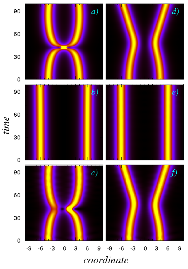
Figure 1: (color online). Evolution in time of a two-hump soliton train in coordinate space. Shown is the evolution in time of the density $\rho(x,t)$ of the attractive system with $N=2000$ bosons and $\lambda_{0}=-0.002$ computed by the popular Gross-Pitaevskii equation on the mean-field level in panels a)-c), and the corresponding dynamics computed on the many-body level in panels d)-f). Panels a) and d) show the dynamics of a $0$-phase symmetric train; Panels b) and e) show the dynamics of a $\pi$-phase anti-symmetric train; Panels c) and f) show the dynamics of a $0$-phase asymmetric train. On the many-body level the forces between the two density humps are weaker, and there is essentially only repulsion and no attraction between them at all but short times. All quantities shown are dimensionless.

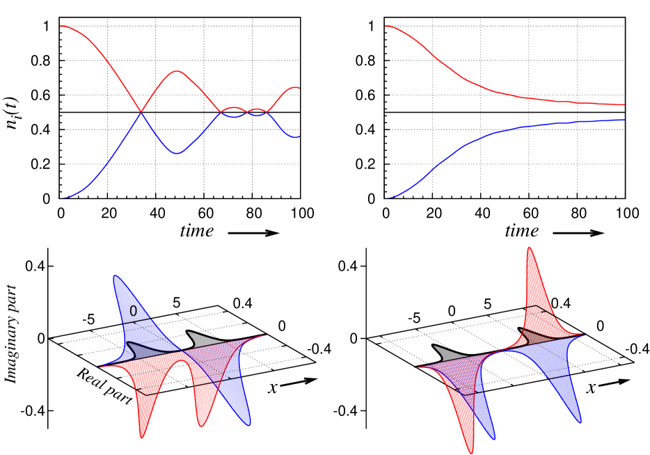
Figure 2: (color online). Death of soliton trains by fragmentation. The upper panels show the occupation numbers of the reduced one-body density matrix of the initially-prepared $0$-phase symmetric (left) and $\pi$-phase anti-symmetric (right) soliton trains of Fig. 1. It is seen that the initially condensed systems become quickly fragmented. The emergence of fragmentation signifies the death of the condensed objects known as bright soliton trains. The lower two panels depict the respective natural orbitals after fragmentation of the initially-prepared $0$-phase symmetric (left) and $\pi$-phase anti-symmetric (right) coherent wave-packets. The two natural orbitals are delocalized functions of ’gerade’ (even) and ’ungerade’ (odd) symmetries. The delocalization of the natural orbitals in combination with the exchange interaction stabilizes the fragmented attractive Bose-Einstein condensates in comparison with the condensed soliton trains. All quantities shown are dimensionless.

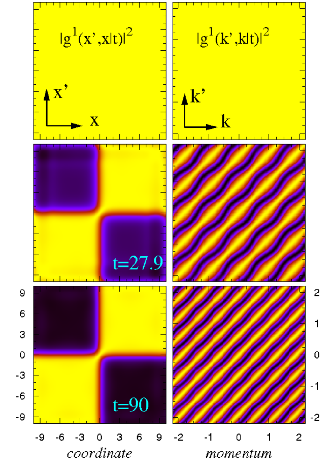
Figure 3: (color online). Detecting the death of soliton trains by means of first-order correlation functions. The upper two panels show the first-order correlation function of the initially-prepared $0$-phase symmetric soliton train of Fig. 1 in coordinate (left) and momentum (right) space. It is completely flat signifying a coherent and condensed state. Within Gross-Pitaevskii theory the system remains condensed for all times; thus the upper two panels represent the first-order correlation function in this case for all times. On the many-body level, the correlation functions are completely different and structured. The pattern emerging in coordinate space indicates no coherence between the two humps (left middle and lower panels), the respective pattern in momentum space represents a fragmented state (right middle and lower panels). Thus, measuring the first-order correlation functions in either coordinate or momentum space provides a direct indication of the death of the soliton train. All quantities shown are dimensionless.

Supplemental Material

Forces between density humps in attractive objects

The time-dependent densities of the evolving initially-prepared bright soliton trains shown in Fig. 1 reveal intricate ”interactions” between the density humps. On the Gross-Pitaevskii (GP) or non-linear Schrödinger equation level (see in this respect Refs. [S1,S2]), $0$-phase symmetric and asymmetric trains show attraction between the density humps, which manifests itself as ”bound” periodic-like motion of the density humps one with respect to the other. The $\pi$-phase anti-symmetric train reveals repulsive interaction between the density humps, which would eventually lead to their increasing separation from each other.

On the many-body level, we have seen in Fig. 1 that repulsive interaction between the density humps eventually prevails, even when the $0$-phase symmetric and asymmetric trains are used as the initially-prepared wave-packets of the attractive system. In this section we would like to contract a simple mean-field model to qualitatively explain the forces between the density humps when soliton trains become fragmented and die.

Let us commence with the development of fragmentation in the $0$-phase symmetric system. The natural orbitals of the decaying soliton train (see left lower panel of Fig. 2) are composed of ’gerade’ (even) and ’ungerade’ (odd) delocalized functions, i.e., they simultaneously exist in the right and left sub-clouds. Oversimplifying the many-body picture of the decay of soliton trains and the development of fragmentation in the system, we can imagine that at every point in time the system is described by a two-orbital mean-field state made of a single permanent (Fock state) $|n_{1},n_{2}\rangle$ [S3] with time-dependent occupation numbers and orbitals. The orbitals comprising this permanent are the above described delocalized even and odd functions. In time, the initially-prepared condensed state $|N,0\rangle$ (built from the delocalized even orbital only, see left panels of Fig. 2) becomes fully fragmented at about $t\approx 34$ (see left upper panel of Fig. 2). Then it is described by the mean-field state $|N/2,N/2\rangle$ (built from both the delocalized even and odd orbitals). Such a fragmetned state has been recently predicted to exist in one dimensional attractive BECs and called fragmenton [S4]. What we would like now to compare within this simplified model is the inter-hump forces in the condensed state $|N,0\rangle$ and fully fragmented state $|N/2,N/2\rangle$. For completeness, the inter-hump forces in the condensed state $|0,N\rangle$ (built from the delocalized odd orbital only, see right panels of Fig. 2) will be registered as well. The delocalized even and odd functions used in our model are conveniently taken as the $0$-phase symmetric and $\pi$-phase anti-symmetric linear combinations ${\cal N}\!\left\{\mathrm{sech}[\gamma(x-x_{0})]\pm\mathrm{sech}[\gamma(x+x_{0})]\right\}$, which reproduce on the mean-field level the limiting cases of the bright soliton trains and the fragmenton.

The energy of the Fock state $|n_{1},n_{2}\rangle$ is given as the expectation value of the Hamiltonian $E(\gamma,x_{0},n_{1},n_{2})=\langle n_{1},n_{2}|\hat{H}|n_{1},n_{2}\rangle$ and depends on the parameters $\gamma$ (inversely proportional to the width of the density humps) and $x_{0}$ (half the separation between the density humps), and on the relative occupation numbers $n_{1}$ and $n_{2}$ ($n_{1}+n_{2}=N$). By taking the derivative $-\frac{\partial E}{\partial x_{0}}$ one immediately arrives at the inter-hump force $F(\gamma,x_{0},n_{1},n_{2})$. The full expression is quite lengthy, but in the large $x_{0}\gamma>2$ limit, i.e., when the humps are well separated from each other, we can prescribe an asymptotic analytical force in the lowest order:

$$F(\gamma,x_{0},n_{1},n_{2})=-\frac{\partial E(\gamma,x_{0},n_{1},n_{2})}{\partial x_{0}}$$

$$=-\frac{4e^{-2\gamma x_{0}}\gamma^{2}}{3N}(n_{1}-n_{2})\left[\lambda_{0}(N-1)(\gamma x_{0}-2)+4\gamma^{2}x_{0}-5\gamma\right].$$

For pure condensed states, i.e., when $n_{1}=N,n_{2}=0$ or $n_{1}=0,n_{2}=N$ with the optimal width $\gamma_{GP}=\lambda_{0}(N-1)/4$, this general expression takes on a very simple form (see in this respect Ref. [S2]):

$$F(\gamma_{GP},x_{0},N)=-\frac{\partial E(\gamma_{GP},x_{0},N)}{\partial x_{0}}=\mp 4e^{-2\gamma_{GP}x_{0}}\gamma_{GP}^{3},$$

where the ”-” corresponds to the $0$-phase symmetric and the ”+” to the $\pi$-phase anti-symmetric two-hump soliton. The damping exponent originates from the residual overlap between the left and right sub-clouds.

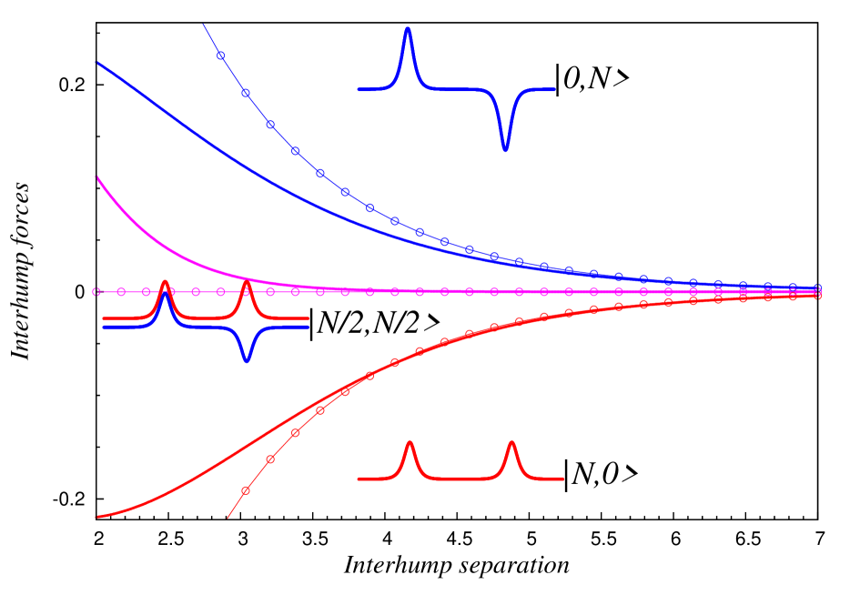
Figure S1: (color online). Forces between density humps in a soliton train and fragmenton. Shown are the forces as a function of inter-hump separation $2x_{0}$ for the $0$-phase symmetric soliton train (attractive force) and the $\pi$-phase anti-symmetric soliton train (repulsive force) for the system of $N=2000$ bosons with $\lambda_{0}=-0.002$. The inter-hump force in a fragmented state built as an admixture of the two soliton trains, $0$-phase symmetric and $\pi$-phase anti-symmetric two-hump solitons (the fragmenton), is much weaker than for the soliton trains themselves, and is repulsive. The full-line curves depict the forces computed numerically, whereas the circle-line curves the asymptotic forces given in Eq. (S1) for the fragmenton and Eq. (S2) for the soliton trains. All quantities shown are dimensionless.

In Fig. S1 we plot the full inter-hump forces and their asymptotic expansions given in Eqs. (S1,S2) as a function of the inter-hump separation $2x_{0}$ for the system of $N=2000$ bosons and $\lambda_{0}=-0.002$ discussed in the main text. In the one limiting case, $n_{1}=N,n_{2}=0$, the force between the density humps of the $0$-phase symmetric soliton train is negative, i.e., attractive. In the other limit, $n_{1}=0,n_{2}=N$, the force between the density humps of the $\pi$-phase anti-symmetric soliton train is positive, i.e., repulsive. For the pure fragmenton $|N/2,N/2\rangle$ this force vanishes asymptotically, because of the $(n_{1}-n_{2})$ prefactor in Eq. (S1). This fact allows us to predict that the inter-hump interaction in the fragmented states is always weaker than in the respective two-hump coherent soliton trains. Interestingly, the residual interaction for the pure fragmenton at a large but not yet asymptotic separation is, nevertheless, repulsive. By going from one limit to another, i.e., by transferring the bosons, say, from the $0$-phase symmetric to the $\pi$-phase anti-symmetric natural orbital, we see that the character of the interaction gradually changes from attractive to repulsive.

Lifetime of two-hump matter-wave soliton trains

In the present section we would like to investigate the scaling of the lifetime of two-hump solition trains with the number of bosons $N$ in the system. We concentrate on the $0$-phase symmetric soliton train. To make the comparison, we keep the GP parameter $\lambda_{0}N=-4$ and inter-hump separation $2x_{0}=8$ fixed to the values used for $N=2000$ throughout the main text. It should be reminded that for a fixed value of $\lambda_{0}N$ the GP dynamics is independent of $N$ (for $N\gg 1$, which is the situation here). Additionally, no fragmentation can be described by the GP equation, of course, and solitons’ lifetime is infinite. Hence, the many-body results presented in this section are to further demonstrate the substantial physical differences between the mean-field and many-body quantum dynamics of 1D attractive Bose systems.

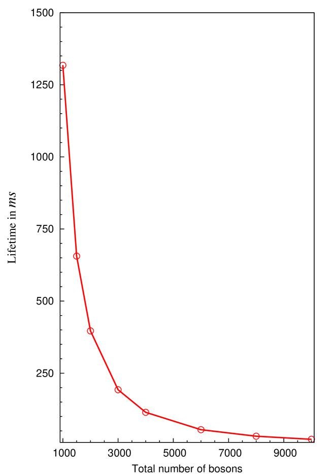
Figure S2: (color online). Lifetime of two-hump soliton trains. Depicted is the lifetime in milliseconds of the $0$-phase symmetric two-hump soliton trains as a function of the total number of bosons $N$ (the solid line connecting the open circles is to guide the eye only). The Gross-Pitaevskii parameter $\lambda_{0}N=-4$ and inter-hump separation $2x_{0}=8$ are kept fixed (corresponding to the system of $N=2000$ bosons with $\lambda_{0}=-0.002$ discussed in the main text). The lifetime decreases roughly quadratically with the number of bosons $N$. It is demonstrated that the death of soliton trains is an ultrafast process that can take place on a time scale which is an order of magnitude shorter than relevant time-scales for current experimental setups (couple of seconds).

Fig. S2 collects the results for the lifetime as a function of $N$. We remind that the lifetime is defined as the time $t$ where the fragmentation ratio of $n_{1}=100\%\times\left(1-\frac{1}{e}\right)=63.21\%$ is reached. Translating from dimensionless to dimension-full quantities, the lifetime of, e.g., the two-hump soliton made of $N=2000$ ⁷Li atoms in a quasi-1D cigar-shaped trap with transverse confinement of $w_{\perp}=2\pi\cdot 800$ Hz is about $400$ milliseconds. This lifetime is short compared to current experimental setups which are a couple of seconds long. It is seen from Fig. S2 that the lifetime decreases roughly quadratically with the number of bosons $N$. For $N=8000$ ⁷Li atoms it is below $50$ milliseconds. All in all, we demonstrate that the death of soliton trains is an ultrafast process that takes place on a time scale which is an order of magnitude shorter than relevant time-scales for current experimental setups.

Momentum distribution of initially-prepared two-hump soliton trains

The density profile of bright soliton trains consists of localized structures. As we have seen in the main text this well-known GP (mean-field) characteristic persists on the many-body level as well, despite the fact that the system becomes fragmented. Consequently, the spatial density of low-dimensional attractive systems is not a straightforward indicator for the development of fragmentation in the system, and hence is not likely to be utilized experimentally to identify it. In this section we would like to augment the indicting information on the death of solitons by reporting the corresponding momentum distribution, see Fig. S3.

The time-dependent momentum distribution $n(k,t)$ obtained by solving the time-dependent GP equation for the two-hump solitons of Fig. 1 is plotted in Fig. S3. In the left upper panel, Fig. S3a, we plot the momentum distribution of the $0$-phase symmetric soliton train. A sharp contrast and oscillatory pattern is seen, which signifies the system being condensed (and coherent, see right upper panel of Fig. 3). As the two density humps approach each other in real space, the corresponding momentum distribution broadens. At the collision point ($t\approx 42$) the momentum distribution is the broadest, since the two colliding clouds momentarily merge into one cloud, yet its maximal value is significantly smaller.

In the left middle panel, Fig. S3b, the momentum distribution of the $\pi$-phase anti-symmetric soliton is depicted. Due to the larger separation between the density humps ($x_{0}=\pm 6$, see Fig. 1b), more maxima and narrower peaks in $n(k,t)$ are seen, in comparison to the soliton train of Fig. S3a (for which $x_{0}=\pm 4$, see Fig. 1a). Furthermore, the momentum distribution is essentially constant for all times shown, as the corresponding spatial density is, due to the initial larger separation between the density humps. Finally, in Fig. S3c, the momentum distribution of the $0$-phase asymmetric soliton train is shown. It also depicts a sharp contrast pattern, but asymmetric. The broadest peaks in $n(k,t)$ correspond to the near collision of the two density humps in real space occuring at about $t\approx 42$ (see Fig. 1c).

We may summarize the following features of the momentum distribution of two-hump solitons computed by the GP theory: (i) appearance of sharp contrast pattern signifying condensation (and coherence), and (ii) the number of peaks seen and their width depend on the initial separation of the density humps in real space (in a reminiscence of a double-slit experiment with light).

On the many-body level, the time-dependent momentum distribution $n(k,t)$ shows essential visual differences from the GP momentum distribution, compare the left and right panels of Fig. S3. In the right upper panel, Fig. S3d, the many-body momentum-distribution dynamics of the initially-prepared $0$-phase symmetric soliton train is shown. For times up to about $t\approx 15$, the sharp contrast pattern characterizing the initially-prepared condensed system survives. Looking at the evolution of the corresponding occupation numbers (see left upper panel of Fig. 2), we see that up to this time the system remains at least $90\%$ condensed. For times longer than just about $t\approx 15$, the many-body momentum distribution almost suddenly becomes ”blared”, in sharp contrast to the GP results. This is yet another signature of the fragmentation of the system. The ”blared” momentum distribution pattern can be anticipated by ”interfering” the momentum distributions carrying the two delocalized even and odd natural orbitals of the fragmented system (see in this respect the left lower panel of Fig. 2). Similarly, the many-body momentum distribution of the initially-prepared $\pi$-phase anti-symmetric wave-packet, Fig. S3e, and the many-body momentum distribution of the initially-prepared $0$-phase asymmetric wave-packet, Fig. S3f, quickly become ”blared”, when fragmentation sets it. We stress that, despite the large separation between the density humps of the $\pi$-phase anti-symmetric wave-packet (see Fig. 1e), the changes in the physics are dramatic.

Summarizing, the momentum distribution of low-dimensional attractive systems initially-prepared as (condensed and coherent) soliton trains quickly loose their contrast and become essentially single-peaked and ”blared”. This consequence and fingerprint of fragmentation should be amenable to experimental detection, and is far better and straightforward indicator of fragmentation than the monitoring of localization in coordinate space.

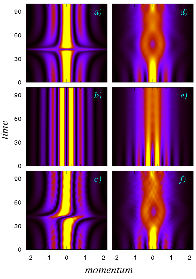
Figure S3: (color online). Evolution in time of a two-hump soliton train in momentum space. Shown is the evolution in time of the momentum distribution $n(k,t)$ of the attractive system of $N=2000$ bosons with $\lambda_{0}=-0.002$ computed by the popular Gross-Pitaevskii equation on the mean-field level in panels a)-c), and the corresponding dynamics computed on the many-body level in panels d)-f). Panels a) and d) show the dynamics of a $0$-phase symmetric train; Panels b) and e) show the dynamics of a $\pi$-phase anti-symmetric train; Panels c) and f) show the dynamics of a $0$-phase asymmetric train. On the mean-field level, panels a)-c), an interference-like sharp-contrast pattern emerges, indicating the two-hump system being condensed. On the many-body level, panels d)-f), the momentum distribution is much more blared, indicating the fragmentation of the system. All quantities shown are dimensionless.

References

- (1) S. Trillo and W. Torruellas (Eds.), Spatial Solitons (Springer, Berlin, 2001).
- (2) G. I. Stegeman and M. Segev, Science 286, 1518 (1999).
- (3) P. A. Ruprecht, M. J. Holland, K. Burnett, M. Edwards, Phys. Rev. A 51, 4704 (1995).
- (4) V. M. Pérez-García, H. Michinel, and H. Herrero, Phys. Rev. A 57, 3837 (1998).
- (5) K. E. Strecker, G. B. Partridge, A. G. Truscott, and R. G. Hulet, Nature 417, 150 (2002).
- (6) L. Khaykovich et al., Science 296, 1290 (2002).
- (7) U. Al Khawaja et al., Phys. Rev. Lett. 89, 200404 (2002).
- (8) L. Salasnich, A. Parola, and L. Reatto, Phys. Rev. Lett. 91, 080405 (2003).
- (9) L. D. Carr and J. Brand, Phys. Rev. Lett. 92, 040401 (2004).
- (10) A. D. Martin, C. S. Adams, and S. A. Gardiner, Phys. Rev. Lett. 98, 020402 (2007).
- (11) E. P. Gross, Nuovo Cimento 20, 454 (1961).
- (12) L. P. Pitaevskii, Zh. Eksp. Teor. Fiz. 40, 646 (1961) [Sov. Phys.–JETP 13, 451 (1961)].
- (13) P. Nozières and D. Saint James, J. Phys. France 43, 1133 (1982).
- (14) A. I. Streltsov, O. E. Alon, and L. S. Cederbaum, Phys. Rev. A 73, 063626 (2006).
- (15) E. J. Mueller, T.-L. Ho, M. Ueda, and G. Baym, Phys. Rev. A 74, 033612 (2006).
- (16) A. I. Streltsov, O. E. Alon, and L. S. Cederbaum, Phys. Rev. Lett. 99, 030402 (2007).
- (17) O. E. Alon, A. I. Streltsov, and L. S. Cederbaum, Phys. Rev. A 77, 033613 (2008).
- (18) J. Grond, J. Schmiedmayer, and U. Hohenester, Phys. Rev. A 79, 021603(R) (2009).
- (19) K. Sakmann, A. I. Streltsov, O. E. Alon, and L. S. Cederbaum, Phys. Rev. Lett. 103, 220601 (2009).
- (20) See EPAPS Document No. xxxx for supplemental physical analysis of the death of soliton trains. For more information on EPAPS, see http://www.aip.org/pubservs/epaps.html.
- (21) A. I. Streltsov, O. E. Alon, and L. S. Cederbaum, Phys. Rev. Lett. 100, 130401 (2008).
- (22) M. Naraschewski and R. J. Glauber, Phys. Rev. A 59, 4595 (1999).
- (23) K. Sakmann, A. I. Streltsov, O. E. Alon, and L. S. Cederbaum, Phys. Rev. A 78, 023615 (2008).
- (24) M. Olshanii, Phys. Rev. Lett. 81, 938 (1998).

References

- (1) G. I. Stegeman and M. Segev, Science 286, 1518 (1999).
- (2) V. I. Karpman and V. V. Solov’ev, Physica D 3, 487 (1981).
- (3) A. I. Streltsov and L. S. Cederbaum, Phys. Lett. A 318, 564 (2003).
- (4) A. I. Streltsov, O. E. Alon, and L. S. Cederbaum, Phys. Rev. Lett. 100, 130401 (2008).