Experimental investigation of the uncertainty principle
in the presence of quantum memory

Abstract

Heisenberg’s uncertainty principle provides a fundamental limitation on an observer’s ability to simultaneously predict the outcome when one of two measurements is performed on a quantum system. However, if the observer has access to a particle (stored in a quantum memory) which is entangled with the system, his uncertainty is generally reduced. This effect has recently been quantified by Berta et al. [Nature Physics 6, 659 (2010)] in a new, more general uncertainty relation, formulated in terms of entropies. Using entangled photon pairs, an optical delay line serving as a quantum memory and fast, active feed-forward we experimentally probe the validity of this new relation. The behaviour we find agrees with the predictions of quantum theory and satisfies the new uncertainty relation. In particular, we find lower uncertainties about the measurement outcomes than would be possible without the entangled particle. This shows not only that the reduction in uncertainty enabled by entanglement can be significant in practice, but also demonstrates the use of the inequality to witness entanglement.

Consider an experiment in which one of two measurements is made on a quantum system. In general, it is not possible to predict the outcomes of both measurements precisely, which leads to uncertainty relations constraining our ability to do so. Such relations lie at the heart of quantum theory and have profound fundamental and practical consequences. They set fundamental limits on precision technologies such as metrology and lithography, and also served as the intuition behind new types of technologies such as quantum cryptography Wiesner (1983); Bennett and Brassard (1984).

The first relation of this kind was formulated by Heisenberg for the case of position and momentum Heisenberg (1927). Subsequent work by Robertson Robertson (1929) and Schrödinger Schrödinger (1930) generalized this relation to arbitrary pairs of observables. In particular, Robertson showed that

$$\Delta R\cdot\Delta S\geq\frac{1}{2}\left|\langle\left[R,S\right]\rangle\right|,$$ (1)

where uncertainty is characterized in terms of the standard deviation $\Delta R$ for an observable $R$ (and likewise for $S$) and the right-hand-side (RHS) of the inequality is expressed in terms of the expectation value of the commutator, $\left[R,S\right]:=RS-SR$, of the two observables.

More recently, driven by information theory, uncertainty relations have been developed in which the uncertainty is quantified using entropy Bialynicki-Birula and Mycielski (1975); Deutsch (1983), rather than the standard deviation. This links uncertainty relations more naturally to classical and quantum information and overcomes some pitfalls of equation (1) pointed out by Deutsch Deutsch (1983). Most uncertainty relations apply only in the case where the uncertainty is measured for an observer holding only classical information about the system. One such relation, conjectured by Kraus Kraus (1987) and subsequently proven by Maassen and Uffink Maassen and Uffink (1988), states that for any observables $R$ and $S$

$$H(R)+H(S)\geq\log_{2}\frac{1}{c},$$ (2)

where $H(R)$ denotes the Shannon entropy Shannon (1949) of the probability distribution of the outcomes when $R$ is measured and the term $1/c$ quantifies the complementarity of the observables. For non-degenerate observables, it is defined by $c:=\max_{r,s}|\langle\Psi_{r}|\Upsilon_{s}\rangle|^{2}$, where $|\Psi_{r}\rangle$ and $|\Upsilon_{s}\rangle$ are the eigenvectors of $R$ and $S$, respectively.

Interestingly, the above relations do not apply to the case of an observer holding quantum information about the measured system. In the extreme case that the observer holds a particle maximally entangled with the quantum system, he is able to predict the outcome precisely for both choices of measurement. This dramatically illustrates the need for a new uncertainty relation.

Recently, Berta et al. Berta et al. (2010) derived such a relation (an equivalent form of this relation had previously been conjectured by Renes and Boileau Renes and Boileau (2009)). The new relation is

$$H(R|B)+H(S|B)\geq\log_{2}\frac{1}{c}+H(A|B),$$ (3)

where the measurement ($R$ or $S$) is performed on a system, $A$, and the additional quantum information held by the observer is in $B$. The Shannon entropy of the outcome distribution is replaced by $H(R|B)$, the conditional von Neumann entropy of the post-measurement state (after $R$ is measured) given $B$. This quantifies the uncertainty about the outcome of a measurement of $R$ given access to $B$ (see the Appendix). This relation is a strict generalization of (2) and features an additional term on the right-hand-side. This term is a measure of how entangled the system $A$ is with the observer’s particle, $B$, expressed via the conditional von Neumann entropy of the joint state, $\rho_{AB}$ of $A$ and $B$ before measurement, $H(A|B)$. Note that this quantity can be negative for entangled states and in this case lowers the bound on the sum of the uncertainties. In particular, if $\rho_{AB}$ is maximally entangled, $H(A|B)=-\log_{2}d$, where $d$ is the dimension of the system. Since $\log_{2}1/c$ cannot be larger than $\log_{2}d$, the RHS of (3) cannot be greater than zero for a maximally entangled state and, as mentioned previously, both $R$ and $S$ are perfectly predictable in such a case, for any observables $R$ and $S$. From a fundamental point of view, this highlights the additional power an observer holding quantum information about the system has compared to an observer holding classical information.

In order to clarify the sense in which an observer holding quantum information can outperform one without, we follow Berta et al. Berta et al. (2010) and consider uncertainty relations in the form of a game between two parties, Alice and Bob: Bob creates a quantum system and sends it to Alice. He can prepare this system as he likes and, in particular, it can be entangled with another particle which he stores in a quantum memory (a device that maintains the quantum coherence of its content). Alice then performs one of two pre-agreed measurements, $R$ or $S$, chosen at random. She then announces the chosen measurement, but not its outcome. Bob’s aim is to minimize his uncertainty (as quantified by the conditional von Neumann entropy) about Alice’s measurement outcome (see Fig. 1).

In this work, we test the new inequality of Berta et al. experimentally using entangled photon states and an optical delay serving as a simple quantum memory. Entanglement allows us to achieve lower uncertainties about both observables than would be possible with only classical information over a wide range of experimental settings. Our work addresses a cornerstone relation in quantum mechanics and, to the best of our knowledge, is the first to test one of its entropic versions. In the past, experiments have come close to the original uncertainty limit Elion et al. (1994); Nairz et al. (2002); LaHaye et al. (2004); Schliesser et al. (2009), but did not involve entangled quantum systems. We also illustrate the practical usefulness of the new inequality by applying it as an effective entanglement witness.

In our experiment, we use polarization-entangled photon pairs generated by spontaneous parametric down-conversion (SPDC) and polarization measurements on the individual photons to test the inequality. Inferring entropic uncertainties from experimental data requires a high level of precision and control over the quantum system under consideration. Polarization-encoded photonic qubits offer this ability, making them a suitable testbed for the new uncertainty relation.

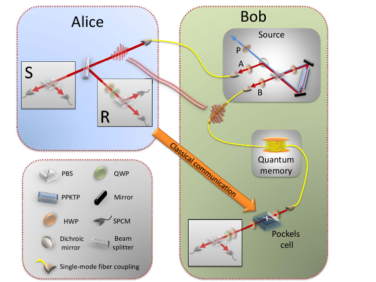
Figure 1: Schematic of the experiment. Entangled photon pairs are created by pumping a periodically poled KTP crystal (PPKTP) inside a Sagnac interferometer and are subsequently fibre-coupled. Half-wave plates (HWP) $P$, $A$, and $B$ are used to prepare arbitrary polarization entangled states (see Appendix for details). One photon is then distributed to Alice who measures one of two observables, $R$ or $S$ (corresponding to different polarization bases). The observable is randomly selected by a 50/50 beamsplitter (BS) which separates the two polarization analyzer modules. The choice of basis is classically transmitted back to Bob, who in the meantime delays his photon in a $50\,\mbox{m}$ single-mode fibre. A fast Pockels cell (PC), which performs the identity when off or a bit flip operation ($\sigma_{x}$) when on, in combination with HWPs adapts Bob’s measurement basis accordingly. The photons are detected using single-photon counting modules (SPCMs) and coincidence events between Alice’s and Bob’s detectors are recorded. Here we have depicted the experiment in the case that Bob measures his photon in the same basis as Alice. In some runs of the experiment, we also perform tomography on Bob’s photon (see main text). QWP, quarter-wave plate; PBS, polarizing beam splitter.

The schematics of the experiment and its connection to the uncertainty game are shown in Fig. 1. Our entangled photon pair source Kim et al. (2006); Fedrizzi et al. (2007); Biggerstaff et al. (2009) can produce an entangled state of the form

$$|\Phi\rangle_{AB}=\cos\zeta|H_{A}H_{B}\rangle+\sin\zeta|V_{A}V_{B}\rangle,$$ (4)

where $|H\rangle$ ($|V\rangle$) denotes a horizontally (vertically) polarized photon and the subscripts label the spatial modes (Alice and Bob, respectively). Control over the parameter $\zeta$ allows us to change the amount of entanglement, characterized by the tangle $\tau$ Hill and Wooters (1997), between the two photons (see Appendix). We can therefore study the inequality for a wide range of different experimental settings.

In our experiment we realize Berta et al.’s uncertainty game, as shown in Fig. 1. The photon sent to Alice is entangled with a second photon which is delayed by sending it through a $50\,\mbox{m}$ single-mode fibre which acts as a quantum memory. This gives Alice sufficient time to measure one of the two observables and to communicate her measurement choice, but not the outcome, to Bob before his photon emerges from the fibre (this is referred to as feed-forward). On Bob’s side, we either perform state tomography, or have Bob measure his photon in the same basis as Alice. In the latter case, a fast Pockels cell Prevedel et al. (2007); Biggerstaff et al. (2009) allows rapid switching between measuring one of two pre-agreed observables. In total, the feed-forward time is on the order of $\sim 150\,\mbox{ns}$. More details regarding the experiment can be found in Fig. 1 and in the Appendix.

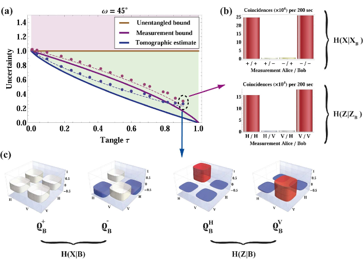
Figure 2: Experimental results. In (a) we plot the left-hand side (LHS) of the new inequality for the case where $R=X$ and $S=Z$. In this case the relative angle, $\omega$, between the observables is $\omega=\pi/4$ ($45^{\circ}$). Varying HWP $S$ in the source allows us to plot the LHS for states with varying entanglement $\tau$. To calculate $H(X|B)+H(Z|B)$ we evaluate the entropies of the conditional single-qubit density matrices of Bob’s qubit which we obtain through quantum state tomography (blue dots). Experimentally, this is achieved by setting the analyzers on Alice’s side to perform measurements in the $\{|H\rangle,|V\rangle\}$ and $\{|+\rangle,|-\rangle\}$ bases. If we also perform projective measurements on Bob’s side we can obtain the entropies $H(X|X_{B})+H(Z|Z_{B})$ (purple dots) directly from the obtained coincidence count rates. Solid lines represent the theoretical bounds for the two entropy calculations, while the dashed lines indicate the simulated performance of the experiment. Note that for conjugate observables, the tomographic estimate coincides with equation (3). For the datapoints associated with the highest entanglement we show the corresponding coincidence count rates in (b) and the reconstructed conditional density matrices in (c). Error bars ($\sim 10^{-4}$) are too small to be seen. See Appendix for details.

The results of our experimental investigation are shown in Figs. 2 and 3. The difference between the original uncertainty principle, equation (2), and Berta et al.’s result, equation (3), is most apparent for the case of maximal entanglement and conjugate observables, i.e. for $R=X$ and $S=Z$. In this scenario, Bob can predict the outcome of Alice’s measurement perfectly, i.e. $H(X|B)+H(Z|B)=0$, which would be impossible if Bob did not have a quantum memory (the RHS of equation (2) has $\log_{2}1/c=1$ for these observables). In fact, for any finite entanglement between Alice’s particle and Bob’s quantum memory we expect to find lower uncertainties than in the case of no entanglement. This trend is clearly observed in Fig. 2 where we vary the entanglement (characterized by the tangle $\tau$) for the case of conjugate observables. This shows that entanglement allows Bob to predict both observables more precisely than without. We also use two different approaches to estimate the LHS of equation (3). The first is a direct determination of $H(X|B)+H(Z|B)$ (the blue, solid line in 2(a)) which requires calculation of the reduced density matrix of Bob’s photon for each of the alternative measurement choices and outcomes, which can in turn be obtained through quantum state tomography James et al. (2001). Alternatively, we can bound the entropies by also performing a projective measurement on Bob’s photon, which allows us to estimate $H(X|X_{B})+H(Z|Z_{B})$ (where $X_{B}$ and $Z_{B}$ are the observables measured by Bob). Since $H(X|B)\leq H(X|X_{B})$, this technique will in general only provide an upper bound on $H(X|B)+H(Z|B)$ and therefore yield a weaker inequality. Its advantage is that it can be estimated with a straightforward experimental test without tomography. In Fig. 2 we show the results of both experimental approaches and we outline the details of the entropy calculations in the Appendix.

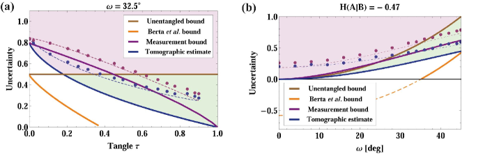
Figure 3: Uncertainties for other experimental settings. In (a) we fix the relative angle between two measurement bases on Alice’s photon at $\omega\approx 0.57$ (32.5^∘). This corresponds to the case where the bound in equation (2) drops to 1/2. Note that here the new uncertainty relation (3) is no longer tight. In (b) we chose a non-maximally entangled state (with $\tau\approx 0.47$) and vary $\omega$, i.e. we fix $S=Z$ and vary $R(\omega)$ from $0$ to $45^{\circ}$. We remark that the conditional entropies $H(R|B)$ and $H(S|B)$ cannot be negative and so, in the cases where the RHS of (3) is negative, the bound $H(R|B)+H(S|B)\geq 0$ should be used instead.

Furthermore we investigate the new uncertainty relation for other choices of observables. Choosing non-conjugate observables lowers the RHS of both inequalities (2) and (3). In Fig. 3(a) we chose the relative angle between the observables, $\omega$, as $\omega\approx 0.57$ ($32.5^{\circ}$) which is where the unentangled bound decreases to $\log_{2}1/c=1/2$. Inequality (3) is not tight in this case, i.e. there is no state for which equation (3) is satisfied with equality. This is seen in Fig. 3, where the tomographic estimate no longer coincides with the Berta et al. bound (as it did for the case of conjugate observables). This scenario places more stringent requirements on the quality of the experiment in order to show that the entanglement allows for lower uncertainties. Nevertheless we find lower entropies than predicted by inequality (2) for sufficiently large entanglement. Discrepancies from the ideal, theoretical bound are mainly due to the imperfect entanglement between the photons. Simulations of the experiment, based on the measured fidelities ($F\approx 0.97$) of our entangled photon pair source and assuming white noise as the dominant source of imperfection, confirm this fact (see dashed lines in Figs. 2 and 3).

In Fig. 3(b), we investigate the new uncertainty relation for a fixed partially entangled state, varying the complementarity of the observables, $c(\omega)$. Again we find good agreement and uncertainties consistent with the new inequality, thereby providing strong evidence for the validity of the new uncertainty principle in practice. Further discussion on the optimization of the entangled states and measurements required to most stringently test the uncertainty principle are described in the Appendix.

We now discuss our experiment and the new inequality in the context of the proposed application as an entanglement witness. Uncertainty relations have been used in the past to derive entanglement witnesses Hofmann and Takeuchi (2003); Gühne (2004). The idea in our case is to use equation (3) to bound $H(A|B)$. Whenever $H(R|B)+H(S|B)<\log_{2}1/c$, we can conclude that $H(A|B)<0$ which is a certificate that $\rho_{AB}$ is entangled. This is readily observed in Figs. 2 and 3: any datapoint below the unentangled bound indicates the presence of entanglement.

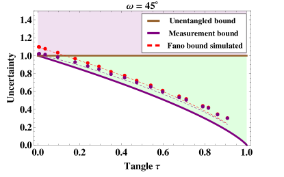
Figure 4: Comparison of the measurement bound and the Fano bound. Here, we compare the two bounds in the case of complementary observables (c.f. Fig. 2(a)). Theoretically, the bounds coincide for this case (purple line). However, in the experiment, we find a slight difference and a worse estimate for the Fano bound (red dots) when compared to our standard method (purple dots). Simulations of the experiment (dashed lines) are in good agreement with the data.

The best entanglement witness is for the case of complementary observables. As can be seen in Fig 2(a), the quality of the witness depends on the technique used. In the case that Bob measures, our experiment detects entanglement for $\tau\geq 0.06\pm 0.01$, which is higher than the analogous bound obtained with tomography, $\tau\geq 0.007\pm 0.003$. However, using tomography requires estimation of more parameters (16 vs 8). An even simpler bound can be obtained using only 2 parameters, which we find to be only slightly weaker as a witness: it detects entanglement for $\tau\geq 0.13\pm 0.02$ (see Appendix Fig. 4).

Significantly, the 2 parameters needed for the simpler bound can be obtained using local measurements, making it a very simple entanglement witness. For single qubits, the merits of this are minor when compared to full tomography. However, more generally the separation between the number of parameters scales like the square of the dimension of the system, making the tomographic estimate infeasible for systems comprising more than a few qubits. We further remark that, although one parameter witnesses exist, these usually require measurement of a joint operator, which can be difficult to implement. In practice these witness operators are often first decomposed into locally measurable parts Terhal (2002); Gühne et al. (2002); Gühne and Toth (2009).

Until recently, all known bounds on the uncertainty an observer can have about the outcomes of measurements on a system applied only to observers holding classical information about the system. Berta et al. have since overcome this limitation, deriving a stronger uncertainty relation which applies when one observer holds quantum information about another system in a quantum memory. In this work, we give the first experimental investigation of this strengthened relation. We demonstrate that entangling the system with a particle in a quantum memory does indeed lead to lower bounds on the uncertainty than is possible without. Our results also quantitatively illustrate the theoretical behaviour of the new uncertainty relation, with discrepancies explained from the measured quality of our source. Future improvements in both photon sources and detectors will allow more precise tests of its bounds. Additionally, since we achieve lower uncertainties than would be possible without entanglement, our experimental setup acts as an effective entanglement witness, and succeeds as such over a wide range of entanglement.

We thank M. Piani for valuable discussions and the Ontario Ministry of Research and Innovation ERA, QuantumWorks, NSERC, OCE, Industry Canada and CFI for financial support. R.P. acknowledges support by MRI and the Austrian Science Fund (FWF).

Appendix A Appendix

A.1 Entropy inference

In this section we give an account of how the quantities appearing in equation (3) can be inferred from the data obtained in the experiment. We begin with the mathematical definition of the relevant quantities. For a density matrix $\rho_{AB}$, the von Neumann entropy is defined by $H(AB):=-\mathrm{tr}(\rho_{AB}\log_{2}\rho_{AB})$, which is conveniently calculated from the eigenvalues, $\{\lambda_{i}\}$, of $\rho_{AB}$ by $H(AB)=H(\{\lambda_{i}\}):=-\sum_{i}\lambda_{i}\log_{2}\lambda_{i}$. For a state $\rho_{AB}$, the conditional entropy of $A$ given $B$ is defined as $H(A|B):=H(AB)-H(B)$, where $H(B)$ is the von Neumann entropy of the reduced density operator, $\rho_{B}:=\mathrm{tr}_{A}\rho_{AB}$. The quantity $H(R|B)$ is the conditional von Neumann entropy of the state

$$\rho_{RB}:=\sum_{r}\left(|\Psi_{r}\rangle\!\langle\Psi_{r}|\otimes\openone\right)\rho_{AB}\left(|\Psi_{r}\rangle\!\langle\Psi_{r}|\otimes\openone\right),$$ (5)

where $R$ corresponds to a measurement on the $A$ system in the orthonormal basis defined by $\{|\Psi_{r}\rangle\}$ (this state is to be interpreted as the post-measurement state after $R$ is measured). It will be convenient to write this in the following form:

$$\rho_{RB}=\sum_{r}p_{r}|\Psi_{r}\rangle\langle\Psi_{r}|\otimes\rho_{B}^{r},$$ (6)

where $p_{r}$ is the probability of obtaining outcome $r$ when $R$ is measured, and $\rho_{B}^{r}$ is the state of the $B$ system when $r$ occurs. The relevant entropy can then be calculated using Nielsen and Chuang (2000)

$$H(R|B)=H\left(\{p_{r}\}\right)+\sum_{r}p_{r}H\left(\rho_{B}^{r}\right)-H\left(\sum_{r}p_{r}\rho_{B}^{r}\right).$$

The entropy $H(S|B)$ can be analogously defined.

The density operators $\{\rho_{B}^{r}\}_{r}$ are obtained by performing tomography on the state of the $B$ system conditioned on a particular outcome (see the next section for details). This generates the tomographic estimate of the uncertainty.

Alternatively, we can estimate $H(R|B)$ by performing a measurement on $B$ in a basis which we denote by $R_{B}$ with outcome $r_{B}$. Since $H(R|B)\leq H(R|R_{B})$, i.e. measurements cannot decrease the entropy, we in general obtain a higher uncertainty. The entropy $H(R|R_{B})$ can be calculated from the resulting joint probability distribution of both measurements, $P(r,r_{B})$, via $H(R|R_{B})=H(\{P(r,r_{B})\})-H(\{P(r_{B})\})$. This gives rise to the measurement bound on the uncertainty.

We also calculate the entropy using the bound $H(R|R_{B})\leq-q_{R}\log_{2}q_{R}-(1-q_{R})\log_{2}(1-q_{R})$ (which comes from Fano’s inequality), where $q_{R}$ is the probability that $r\neq r_{B}$. This gives rise to the Fano bound on the uncertainty. See the below for more information.

In the experiment we investigate the uncertainties for two-qubit states with Schmidt coefficients $\cos\zeta$ and $\sin\zeta$. Such states have conditional von Neumann entropy $H(A|B)=-H(\{\cos^{2}\zeta,\sin^{2}\zeta\})$ and tangle $\tau=\sin^{2}2\zeta$.

A.2 Experiment

In our experiment, we generate the entangled photons pairs using type-II spontaneous parametric down-conversion (SPDC). A 0.7 mW diode laser at 404 nm pumps a 25 mm periodically-poled KTiOPO₄ (PPKTP) crystal in a Sagnac configuration, emitting entangled photons which are subsequently single-mode fibre-coupled after 3 nm bandpass interference filters (IF) Kim et al. (2006); Fedrizzi et al. (2007); Biggerstaff et al. (2009). Typically we observe a coincidence rate of 15 kHz directly at the source. A half-wave plate (HWP) $P$ before the Sagnac interferometer controls the pump polarization and therefore allows us to precisely control $\zeta$ in equation (4) and hence the entanglement of the generated state. Additional HWPs at the outputs of the fibres rotate the entangled state into the desired Schmidt basis $|\theta\rangle$ (see below). Photons are detected by single-photon counting modules (SPCM) and their frequencies are recorded using a multichannel logic with a coincidence window of 3 ns.

On Alice’s side, two polarization analyzer modules, each consisting of a PBS preceded by a QWP and HWP, are separated by a 50/50 beamsplitter. One of them is set to measure in the $\{|H\rangle,|V\rangle\}$ basis while the other can be set to measure at some chosen angle in the X-Z plane, i.e. $\{|\omega\rangle,|\omega^{\bot}\rangle\}$ where the $\omega$ in $|\omega\rangle=\cos\omega|H\rangle+\sin\omega|V\rangle$ is the angle of the linear polarization.

The other down-converted photon is meanwhile delayed in a 50 m single-mode optical fibre spool, which is long enough to execute the measurements on Alice’s side and communicate (feed-forward) her chosen basis to Bob. Depending on the basis, Bob switches between two analyzer bases, $R$ and $S$. This is achieved by using a fast RbTiOPO₄ (RTP) Pockels cells (PC), aligned so as to perform a $\sigma_{x}$ (X) operation Prevedel et al. (2007); Biggerstaff et al. (2009). HWPs before and after the PC allow to adapt the switchable analyzer bases. Therefore, after passing the PC, Bob’s photon is effectively measured in the $\{|\omega\rangle,|\omega^{\bot}\rangle\}$ ($\{|H\rangle,|V\rangle\}$) basis when the PC is on (off).

The experiment itself is performed as follows. At the start of each run, quantum state tomography James et al. (2001); Langford et al. (2005) is performed on the entangled photon pair. We record coincidences between Alice’s reflected arm of the BS and Bob’s polarization analyzer following the switched off PCs. Coincidence measurements were integrated over $5\,\mbox{s}$ for a tomographically over-complete set of measurements, comprising all combinations of the six eigenstates of $X$, $Y$, and $Z$ on Alice’s and Bob’s qubit, respectively. Using an iterative technique Ježek et al. (2003) we reconstruct the density matrix $\rho_{\text{AB}}^{\text{exp}}$, from which we infer the tangle $\tau$ of our state. We then set the analyzers on Alice’s side to the $\{|H\rangle,|V\rangle\}$ ($\{|\omega\rangle,|\omega^{\bot}\rangle\}$) basis in the transmitted (reflected) arm of the BS and perform conditional single-qubit tomography on Bob’s photon, from which we calculate $H(R(\omega)|B)+H(Z|B)$. Finally, Bob’s analyzer is set to the $\{|H\rangle,|V\rangle\}$ basis which allows us to calculate $H(Z|Z_{B})$ and $H(R(\omega)|R_{B}(\omega))$ directly from the coincidence counts. Stepwise repetition of this procedure for varying $\zeta$ or $\omega$ leads to the data presented in Figs. 2 and 3.

A.3 State and measurement optimization

Our aim is to rigorously test the validity of the new uncertainty relation (3) in an experimental setting. However, it is not the case that for all pairs of measurements there exists a state which saturates the bound. Likewise, it is not the case that for all states the bound can be saturated by some pair of measurements. Hence, in order to probe the bound, we try to observe the minimum uncertainties possible (i.e. the minimum left-hand side attainable). In this section, we show how to achieve this minimum.

We start by considering the new uncertainty relation in the case where the state of the system and memory is a pure two-qubit state. Without loss of generality, we can assume $S$ is a measurement in the $\{|H\rangle,|V\rangle\}$ basis and $R$ is a measurement in the $\{\cos\omega|H\rangle+\sin\omega|V\rangle,-\sin\omega|H\rangle+\cos\omega|V\rangle\}$ basis, which we denote $\{|\omega\rangle,|\omega^{\bot}\rangle\}$. The pure two-qubit state $|\Phi_{AB}\rangle$ on which we apply the relation can be written in its Schmidt basis

$$|\Phi_{AB}\rangle=\cos\zeta|\theta\rangle_{A}\otimes|\theta\rangle_{B}+\sin\zeta|\theta^{\bot}\rangle_{A}\otimes|\theta^{\bot}\rangle_{B},$$

where $|\theta\rangle$ and $|\theta^{\bot}\rangle$ are orthogonal states, which we generically write as $|\theta\rangle=\cos\theta|H\rangle+e^{i\varphi}\sin\theta|V\rangle$ and $|\theta^{\bot}\rangle$ being the orthogonal state. Using the binary entropy function $h_{2}(p):=-p\log_{2}p-(1-p)\log_{2}(1-p)$, we can write out the terms in equation (3) as

$$H(A|B) = -h_{2}(\cos^{2}\zeta)$$

$$c = \max\left(\cos^{2}\omega,\,\sin^{2}\omega\right)$$

$$H(R|B) = h_{2}\Big{(}\frac{1}{2}(1-\cos(2\zeta)(\cos(2\omega)\cos(2\theta)$$

$$+\sin(2\omega)\sin(2\theta)\cos\varphi))\Big{)}-h_{2}(\cos^{2}\zeta)$$

$$H(S|B) = h_{2}\left(\frac{1}{2}(1-\cos(2\zeta)\cos(2\theta))\right)-h_{2}(\cos^{2}\zeta).$$

For fixed entanglement $H(A|B)$, i.e. fixed $\zeta$, and a given complementarity between the observables, i.e. fixed $\omega$, we want to find the corresponding entangled state $|\Phi_{AB}\rangle$ that achieves the minimum uncertainty, so that we can get closest to the bound given by equation (3).

A.3.1 Conjugate observables

This is the case $R=X$, i.e. $\omega=\frac{\pi}{4}$ so that $H(R|B)$ reduces to

$$H(R|B)=h_{2}\left(\frac{1}{2}(1-\cos(2\zeta)\sin(2\theta)\cos\varphi)\right)-h_{2}(\cos^{2}\zeta).$$

The minimum over $\varphi$ is then for $\varphi=0$. We then have

$$H(R|B)+H(S|B)=h_{2}\left(\frac{1}{2}(1-\cos(2\zeta)\sin(2\theta))\right)$$

$$\quad+h_{2}\left(\frac{1}{2}(1-\cos(2\zeta)\cos(2\theta))\right)-2h_{2}(\cos^{2}\zeta).$$

From the form of $h_{2}(p)$, it is clear that the minimum over $\theta$ occurs for $\theta=0$ or $\theta=\frac{\pi}{4}$ and has the value $1-h_{2}(\cos^{2}\zeta)$. In other words, for the case $R=X$, $S=Z$, and fixed $H(A|B)$, to minimize the uncertainty, the best choice of state is $|\Phi\rangle=\cos\zeta|HH\rangle+\sin\zeta|VV\rangle$. The parameter $\zeta$ is related to the tangle $\tau$ through the relation $\tau=\sin^{2}2\zeta$ and can be conveniently set by HWP $P$ in our photon pair source. Note that, in this case, the bound given by equation (3) is achievable. This is the blue, solid line (tomographic bound) in Fig. 2(a).

A.3.2 General observables

In the general case of arbitrary $R$, the optimal $\varphi$ can be $0$ or $\pi$ depending on the other parameters. However, we can always take $\varphi=0$ and note that the minimum over $\theta$ accounts for the two possibilities (taking $\varphi$ from $0$ to $\pi$ is equivalent to taking $\theta$ to $\pi-\theta$, in terms of the entropies). The task is then to minimize

$$h_{2}\left(\frac{1}{2}\left(1-\cos(2\zeta)(\cos(2\omega)\cos(2\theta)+\sin(2\omega)\sin(2\theta))\right)\right)$$

$$+h_{2}\left(\frac{1}{2}(1-\cos(2\zeta)\cos(2\theta))\right)-2h_{2}(\cos^{2}\zeta)$$

on $\theta$ for fixed $\zeta$ and $\omega$. For a wide range of parameters, the minimum occurs for $\theta=\omega/2$, so that the best entangled state is aligned “in between” the $Z$ axis and the axis of $R$. However, when the measurements are close to complementary (i.e. $\omega\approx\frac{\pi}{4}$), the minimum can occur at $\theta=0$ (as in the case of perfectly complementary observables).

The optimal measurement of Bob is not necessarily the same as that of Alice in the general case. In general, the best measurement setting on Bob’s side can be found by numerical optimization. However, in the cases investigated here, choosing the same measurement on both sides provides an entropy close to that of the optimal with the difference being insignificant when compared to experimental errors.

References

- Wiesner (1983) S. Wiesner, Sigact News 15, 78 (1983).
- Bennett and Brassard (1984) C. H. Bennett and G. Brassard, Proceedings of IEEE International Conference on Computers, Systems and Signal Processing, Bangalore, India pp. 175–179 (1984).
- Heisenberg (1927) W. Heisenberg, Z. Phys. 43, 172 (1927).
- Robertson (1929) H. P. Robertson, Phys. Rev. 34, 163 (1929).
- Schrödinger (1930) E. Schrödinger, Proceedings of The Prussian Academy of Sciences Physics-Mathematical Section XIX, 296 (1930).
- Bialynicki-Birula and Mycielski (1975) I. Bialynicki-Birula and J. Mycielski, Communications in Mathematical Physics 44, 129 (1975).
- Deutsch (1983) D. Deutsch, Physical Review Letters 50, 631 (1983).
- Kraus (1987) K. Kraus, Phys. Rev. D 35, 3070 (1987).
- Maassen and Uffink (1988) H. Maassen and J. B. Uffink, Phys. Rev. Lett 60, 1103 (1988).
- Shannon (1949) C. E. Shannon, Bell System Technical Journal 28, 656 (1949).
- Berta et al. (2010) M. Berta, M. Christandl, R. Colbeck, J. M. Renes, and R. Renner, Nature Physics 6, 659 (2010).
- Renes and Boileau (2009) J. M. Renes and J.-C. Boileau, Phys. Rev. Lett. 103, 020402 (2009).
- Elion et al. (1994) W. Elion, M. Matters, U. Geigenmuller, and J. Mooij, Nature 371, 594 (1994), ISSN 0028-0836.
- Nairz et al. (2002) O. Nairz, M. Arndt, and A. Zeilinger, Phys. Rev. A 65, 032109 (2002).
- LaHaye et al. (2004) M. D. LaHaye, O. Buu, B. Camarota, and K. C. Schwab, Science 304, 74 (2004).
- Schliesser et al. (2009) A. Schliesser, O. Arcizet, R. Riviere, G. Anetsberger, and T. J. Kippenberg, Nature Physics 5, 509 (2009), ISSN 1745-2473.
- Hofmann and Takeuchi (2003) H. F. Hofmann and S. Takeuchi, Phys. Rev. A 68, 032103 (2003).
- Gühne (2004) O. Gühne, Phys. Rev. Lett. 92, 117903 (2004).
- Kim et al. (2006) T. Kim, M. Fiorentino, and F. N. C. Wong, Phys. Rev. A 73, 012316 (2006).
- Fedrizzi et al. (2007) A. Fedrizzi, T. Herbst, A. Poppe, T. Jennewein, and A. Zeilinger, Opt. Express 15, 15377 (2007).
- Biggerstaff et al. (2009) D. N. Biggerstaff, R. Kaltenbaek, D. R. Hamel, G. Weihs, T. Rudolph, and K. J. Resch, Phys. Rev. Lett. 103, 240509 (2009).
- Hill and Wooters (1997) S. Hill and W. K. Wooters, Phys. Rev. Lett. 78, 5022 (1997).
- Prevedel et al. (2007) R. Prevedel, P. Walther, F. Tiefenbacher, P. Böhi, R. Kaltenbaek, T. Jennewein, and A. Zeilinger, Nature 445, 65 (2007).
- James et al. (2001) D. James, P. Kwiat, W. Munro, and A. White, Phys. Rev. A 64, 52312 (2001).
- Terhal (2002) B. M. Terhal, Theor. Comp. Sc. 287, 313 (2002).
- Gühne et al. (2002) O. Gühne, P. Hyllus, D. Bruß, A. Ekert, M. Lewenstein, C. Macchiavello, and A. Sanpera, Phys. Rev. A 66, 062305 (2002).
- Gühne and Toth (2009) O. Gühne and G. Toth, Physics Reports 474, 1 (2009), ISSN 0370-1573.
- Nielsen and Chuang (2000) M. A. Nielsen and I. L. Chuang, Quantum Computation and Quantum Information (Cambridge University Press, Cambridge, 2000).
- Langford et al. (2005) N. K. Langford, T. J. Weinhold, R. Prevedel, K. J. Resch, A. Gilchrist, J. L. O’Brien, G. J. Pryde, and A. G. White, Phys. Rev. Lett. 95, 210504 (2005).
- Ježek et al. (2003) M. Ježek, J. Fiuráek, and Z. Hradil, Phys. Rev. A 68, 012305 (2003).