Neutral mode heat transport and fractional quantum Hall shot noise

Abstract

We study nonequilibrium edge state transport in the fractional quantum Hall regime for states with one or several counter-propagating neutral modes. We consider a setup in which the neutral modes are heated by a hot spot, and where heat transported by the neutral modes causes a temperature difference between the upper and lower edges in a Hall bar. This temperature difference is probed by the excess noise it causes for scattering across a quantum point contact. We find that the excess noise in the quantum point contact provides evidence for counter-propagating neutral modes, and we calculate its dependence on both the temperature difference between the edges and on source drain bias.

Many of the peculiar properties of quantum Hall (QH) systems can be attributed to the existence of quasi-one-dimensional electronic states along the perimeter of the sample, the so-called edge states halperin . In the integer quantum Hall regime edge states can be modelled by non-interacting electrons, and the physics of edge states is capable of describing numerous transport experiments if the Landauer transport theory is generalized to incorporate multiple terminals buettiker . In the fractional QH regime interactions play an essential role, and edge states must be described as Luttinger liquids wen , in some cases with excitations propagating both with and against the orientation imposed by the magnetic field. For instance, in the case of filling fraction $\nu=2/3$ two counter-propagating edge modes are predicted wen ; macdonald , which would give rise to non-universal Hall and two-terminal conductances. Experimentally, however, conductances are quantized and a counter-propagating charge mode was not observed ashoorietal . This problem is resolved by taking into account that in the presence of random edge scattering the $\nu=2/3$ edge undergoes reconstruction into a disorder-dominated phase with a single downstream-propagating charge mode and a single upstream-propagating neutral mode kfp .

Interest in neutral quantum Hall edge modes was revived because one or several neutral Majorana edge mode is expected to encode the non-abelian statistics of the QH state at filling fraction $\nu=5/2$ review ; MR ; apf1 ; apf2 ; OvWe08 . Neutral quantum Hall modes are notoriously difficult to observe as they do not participate in charge transport. Recently, experimental evidence for neutral modes was presented by demonstrating that injection of a DC current can influence the low frequency noise generated at a quantum point contact (QPC) located upstream of the contact where the current is injected heiblum . Partitioning of a DC current by a QPC and the influence of downstream heat transport on a second QPC was studied both experimentally Granger+09 and theoretically FeLi08 ; GrDa09 .

In this Letter, we theoretically analyze a setup akin to that of Ref. heiblum and find that a current injected into a quantum Hall mode downstream of a QPC indeed enhances the charge noise due to scattering at the QPC. In our model, this happens because the injected current causes a hot spot in the contact and, in the presence of one or several neutral modes propagating in the direction opposite to that imposed by the magnetic field for charge pulses, heat is conducted from the contact to the QPC and gives rise to excess noise in the current scattered across the QPC. When the model is generalized to the non-abelian $\nu=5/2$ quantum Hall state the enhancement of the charge noise, also observed in this state heiblum , limits the possible descriptions of the state to those that support counter-propagating neutral modes, namely, the anti-Pfaffian apf1 ; apf2 and an edge reconstrcted Pfaffian state Wan+06 ; OvWe08 .

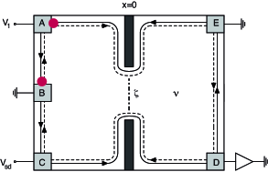
Figure 1: (color online) Schematic diagram of the considered setup. The magnetic field is oriented so that charge transport along the edge (solid black lines) occurs with the counterclockwise chirality. There is one or several neutral modes (dashed lines) propagating clockwise, and the dash-dotted line denotes backscattering at the constriction. Hot spots caused by a finite $V_{1}$ are indicated by red dots.

We consider a multi-terminal Hall bar geometry (see Fig.1), and we assume that the bulk is in a quantized Hall state with filling fraction $\nu$ with one or several neutral modes propagating in the direction opposite to that of the charge mode. The two edges between which scattering takes place are located on the upper and lower sides of the Hall bar, and are labeled $j=1$ and $j=2$, respectively. While contacts $B$ and $E$ are grounded, contacts $A$ and $C$ have tuneable electrochemical potentials, $eV_{1}$ and $eV_{\rm sd}$, where $e$ here is the electron charge. Current and noise are measured at contact $D$. The two dark pads at $x=0$ represent top gates, which form a gated constriction that pinches the edge channels together and causes backscattering of quasiparticles (QPs) between the edges.

The source-drain bias at contact $C$ raises the chemical potential of the emanating charge mode in the bottom edge and gives rise to a current $\nu(e^{2}/h)V_{sd}$ impinging on the QPC. A finite $V_{1}$ gives rise to an electrical current $I_{1}=\nu(e^{2}/h)V_{1}$ flowing from contact $A$ to contact $B$. We note that in the experimentally relevant regime where Hall and longitudinal conductances are quantized, no electrical current is flowing from contact $A$ to contact $E$, and that the expectation value of the neutral mode decays quickly away from contact $A$. While the total electrical power supplied to the system is $I_{1}V_{1}$, the electrical energy current flowing from contact $A$ to contact $B$, which is dissipated in a hot spot at contact $B$, is only $I_{1}V_{1}/2$ ChHa . The rest of the electical power is dissipated at a second hot spot, located on the upstream side of contact $A$. Here, high energy electrons “fall into” the incoming edge mode and fill it up to the electrochemical potential $eV_{1}$ of contact $A$, dissipating energy in the process. The heat generated in this process has to be transported away, which may happen through the wire connecting to contact $A$ or some other cooling mechanism. In general, the equilibrium temperature $T_{A}$ in the region of the hot spot will grow monotonically with the current $I_{1}$. Under the specific assumption that the cooling mechanism is of electronic origin and follows the Wiedemann-Franz law, one would find that the temperature $T_{A}$ at contact $A$ is given by $T_{A}=\sqrt{T_{0}^{2}+I_{1}V_{1}/GL}$, where $T_{0}$ denotes the temperature of the electron bath contact $A$ is connected to, $G$ the conductance of contact $A$ to that electron bath, and $L$ the Lorenz number. In the limit where $T_{A}\gg T_{0}$, one finds $T_{A}\propto I_{1}$.

If the upper edge has at least one counter-propagating neutral mode, heat transport from contact $A$ to the QPC will be possible and the hot spot at contact $A$ will give rise to an increased temperature $T_{1}$ of the upper edge at the QPC. Denoting the temperature of the lower edge by $T_{2}$, the fact that $T_{1}>T_{2}$ due to injection of a current $I_{1}$ into contact $A$ gives rise to enhanced scattering at the QPC and an enhancement of current noise. This description is justified because on the scale of the inelastic mean free path $\ell_{\sigma}$ equilibration between the charge mode and neutral mode(s) takes place kfnm . If the distance between contact $A$ and the QPC is much larger than $\ell_{\sigma}$, charge and neutral modes have a common temperature $T_{1}$ at the QPC. In addition, we make the realistic assumption (verified for the random 2/3-edge) that $\ell_{\sigma}\gg L_{T}$, where $L_{T}=u_{\sigma}/T$ denotes the thermal length. As the edge correlations describing scattering at the QPC decay on the scale $L_{T}$, the inequality $L_{T}\ll\ell_{\sigma}$ implies that a possible temperature gradient on the scale $\ell_{\sigma}$ will not influence current and noise at the QPC, and we can consider an effective model in which backscattering at the constriction is described by assigning a common temperature $T_{1}$ to both charge and neutral modes on the upper edge. The relation between the temperatures $T_{1}$ and $T_{A}$ depends on the thermal Hall conductance $K_{H}$ of the edge. For a vanishing $K_{H}=0$ (realized for a random 2/3-edge), heat transport along the edge is diffusive, and $T_{1}<T_{A}$. The exact value of $T_{1}$ depends on microscopic details like the distances between the QPC to contacts $A$ and $E$ and the amount of scattering between different edge modes. For a $K_{H}<0$ (e.g. for the anti-Pfaffian edge apf1 ; apf2 one finds $K_{H}=-1/2$), heat transport is ballistic and $T_{1}=T_{A}$. In the following, we present a calculation for current and noise at contact $D$ as a function of both source-drain voltage $V_{sd}$ and “neutral” voltage $V_{1}$ for the random $2/3$-edge. We later generalize our formulas to account for general states.

In the presence of disorder, edge excitations of the $\nu=2/3$ fractional QH liquid are predicted to reflect the physics of a stable zero-temperature disorder-dominated fixed point kfp ; kfnm . At the fixed point, each edge consists of a set of decoupled charge ($\phi_{\rho}$) and neutral ($\phi_{\sigma}$) modes that propagate in opposite directions. The effect of random elastic scattering can be incorporated into the neutral mode by fermionizing it, eliminating the scattering term by a spatially random SU(2) transformation, and rebosonizing. At the fixed point, the appropriate real-time Lagrangian density is given by $\mathscr{L}_{0}=\sum_{j=1,2}(\mathscr{L}_{\rho j}+\mathscr{L}_{\sigma j})$, where

$$\mathscr{L}_{\rho j} = \partial_{x}\phi_{\rho j}((-)^{j-1}\partial_{t}-u_{\rho}\partial_{x})\phi_{\rho j}/2\nu$$

$$\mathscr{L}_{\sigma j} = \partial_{x}\phi_{\sigma j}((-)^{j}\partial_{t}-u_{\sigma}\partial_{x})\phi_{\sigma j}/4\ \ .$$ (1)

Here, $u_{\rho}$ ($u_{\sigma}$) is the charge (neutral) mode velocity, and we use units where $\hbar=1=k_{B}$. The charge and neutral modes are coupled by a spatially random interaction term $\mathscr{L}_{\rho\sigma}=u_{int}(x)\partial_{x}\phi_{\rho j}\partial_{x}\phi_{\sigma j}$. The coupling $u_{int}(x)$ is uncorrelated on spatial scales large compared to the elastic mean free path $\ell_{0}$, and we denote its variance by $W_{int}$. This term decays under the renormalization group (RG) flow kfnm and vanishes in the zero temperature limit, giving rise to the fixed point Lagrangian Eq. (1). At finite temperature, the RG flow is stopped at the thermal length $L_{T}$, and the coupling between the charge and neutral modes gives rise to an inelastic mean free path $\ell_{\sigma}^{-1}\sim W_{\rm int}T^{2}$ kfnm . At low temperatures $\ell_{\sigma}$ is parametrically larger than the thermal length $L_{T}$ over which the bosonic Green function decays. Hence, the local bosonic expectation values needed to evaluate the probability of QP scattering across the QPC can be evaluated using the fixed point Lagrangian Eq. (1).

Figure 2: Nonequilibrium excess noise for the random $\nu=2/3$ edge (upper panel) and the random $\nu=5/2$ anti-Pfaffian edge (lower panel) as a function of the temperature difference, $\Delta T=T_{1}-T_{2}$, between the two edges. The solid, dashed and dotted curves are for $T_{2}=0.001$, $T_{2}=0.002$, and $T_{2}=0.003$, respectively. Tunneling amplitudes and temperature are in units of the UV cutoff $\tau_{c}^{-1}$, and the noise is in units of the Nyquist noise with $T_{2}=0.001$. Tunneling amplitudes have been chosen so that the QPC has a transmission of 0.9 at $T_{1}=T_{2}=0.001$.

We now outline the formalism which enables us to compute the current and noise. Upon integrating out all fluctuations away from the defect site (at $x=0$) in the action $S_{0}=\int dt\mathscr{L}_{0}$, we arrive at an effective action in terms of the local fields $q_{\rho j}(t):=\phi_{\rho j}(x=0,t)$ and $q_{\sigma j}(t):=\phi_{\sigma j}(x=0,t)$ kfnoise

$$S^{K}_{{\rm eff}} = \frac{i}{4\pi}\sum_{m=\rho,\sigma}\sum_{j=1,2}\int\frac{d\omega}{2\pi}Q_{mj}^{\dagger}(\omega)\hat{d}_{mj}^{-1}(\omega)Q_{mj}(\omega)$$ (4)

$$+ \int\frac{d\omega}{\pi}\Gamma^{\dagger}(\omega)\left(\begin{array}[]{cc}0&\frac{\omega}{2\pi}\\ \frac{\omega}{2\pi}&\frac{\omega}{2\pi}\coth\left(\frac{\omega}{2T_{2}}\right)\end{array}\right)Q_{\rho 2}(\omega)$$

$$+ \int\frac{d\omega}{2\pi}\,\Gamma^{\dagger}(\omega)\left(\begin{array}[]{cc}0&-\frac{\omega\nu}{4\pi}\\ \frac{\omega\nu}{4\pi}&-\frac{\omega\nu}{4\pi}\coth\left(\frac{\omega}{2T_{2}}\right)\end{array}\right)\Gamma(\omega).$$ (7)

To harness the nonequilibrium nature of the problem, the above action has been mapped onto the Keldysh time-loop contour kamenev ; rammerbook . Upper case letters are used to denote two-component fields in Keldysh space, i.e. $B=(b^{\rm cl},\,b^{\rm q})^{T}$ for a general bosonic field $b$. The components are labeled “classical” and “quantum”, which relate to the fields on the forward ($+$) and backward ($-$) branches of the Keldysh contour via $b^{\rm cl,q}=(b^{+}\pm b^{-})/\sqrt{2}$. $\hat{d}_{mj}(\omega)$ is the local Keldysh matrix propagator for mode $m\in\{\rho,\sigma\}$ and edge $j\in\{1,2\}$. Each propagator has the Keldysh causality structure kamenev , and contains retarded ($R$), advanced ($A$) and Keldysh ($K$) Green’s functions. Here, the retarded Green’s functions are given by $d^{R}_{\rho j}(\omega)=[d^{A}_{\rho j}(\omega)]^{*}=-i\nu/2\omega$ and $d^{R}_{\sigma j}(\omega)=[d^{A}_{\sigma j}(\omega)]^{*}=-i/\omega$. The Keldysh Green’s functions can be obtained via the fluctuation-dissipation relation, $d^{K}_{mj}(\omega)=\coth(\omega/2T_{j})(d^{R}_{mj}(\omega)-d^{A}_{mj}(\omega))$. In Eq.(4), we have also introduced $\Gamma(\omega)=(b(\omega),\,e\mu(\omega))^{T}$. Its classical component, $b(\omega)$, is related to the external source-drain voltage through $\partial_{t}b(t)=\sqrt{2}eV_{\rm sd}$. Its quantum component is the source field, $\mu(\omega)$, which is used to generate all the cumulants of the current operator defined on the lower edge at position $x_{0}>0$, i.e. $I(x_{0},t)=eu_{\rho}\partial_{x}\phi_{\rho 2}(x_{0},t)/\sqrt{2\pi}$. In the above, we have assumed that the period of the AC source-drain bias is much longer than the time for ballistic transport through the device, thus, effectively allowing one to take the limit $x_{0}\rightarrow 0^{+}$. The limit entails no effect on our results which only focus on the steady steady current and the low frequency noise.

Figure 3: Nonequilibrium excess noise for the random $\nu=2/3$ edge (upper panel) and the random $\nu=5/2$ anti-Pfaffian edge (lower panel) as a function of the source-drain voltage. The bottom edge temperature is fixed at $T_{2}=0.001$, and the top edge temperature $T_{1}=0.001$ (Solid); $T_{1}=0.0015$ (Dashed); $T_{1}=0.002$ (Dot-dashed); and $T_{1}=0.0025$ (Dotted). Tunneling amplitudes and temperature are in units of the UV cutoff $\tau_{c}^{-1}$, and the noise is in units of the Nyquist noise with $T_{2}=0.001$. Tunneling amplitudes have been chosen so that the QPC has a transmission of 0.9 at $T_{1}=T_{2}=0.001$.

For $\nu=2/3$, the most relevant operator which describes QP tunneling between the edges is not unique. In particular, there are three tunneling terms with the same scaling dimension, two of which involve tunneling of $e/3$ QPs and another involving $2e/3$ QPs. Since tunneling takes place at $x=0$, the tunneling Lagrangians can be expressed in terms of the local fields. On the Keldysh contour, the action is given by $S^{K}_{T}=-i\int dt\,[L^{+}_{T}-L^{-}_{T}]$, where

$$L^{\alpha}_{T} = -\zeta_{1}\cos\left[\left(q^{\alpha}_{\rho 1}(t)-q^{\alpha}_{\sigma 1}(t)-q^{\alpha}_{\rho 2}(t)+q^{\alpha}_{\sigma 2}(t)\right)/2\right]$$

$$-\zeta_{2}\cos\left[\left(q^{\alpha}_{\rho 1}(t)+q^{\alpha}_{\sigma 1}(t)-q^{\alpha}_{\rho 2}(t)-q^{\alpha}_{\sigma 2}(t)\right)/2\right]$$

$$-\zeta_{3}\cos\left(q^{\alpha}_{\rho 1}(t)-q^{\alpha}_{\rho 2}(t)\right),$$

and $\zeta_{i}$ are the tunneling amplitudes. Here, $\alpha\in\{+,-\}$ labels the forward and backward branches of the Keldysh contour.

The terms linear in $\Gamma(\omega)$ in Eq.(4) can be eliminated by performing the shift

$$Q_{\rho 2}(\omega)\rightarrow Q_{\rho 2}(\omega)-\left(\begin{array}[]{cc}1&\coth(\omega/2T_{2})\\ 0&-1\end{array}\right)\nu\Gamma(\omega).$$ (9)

The corresponding shift in the $+$-$-$ basis, relevant for the scattering terms in Eq.(Neutral mode heat transport and fractional quantum Hall shot noise), is $q^{\alpha}_{\rho 2}(t)\rightarrow q^{\alpha}_{\rho 2}(t)-e^{*}V_{\rm sd}t-(e^{*}/\sqrt{2})(P^{\alpha}\mu)(t)$, where the effective charge $e^{*}=\nu e$ and $(P^{\alpha}\mu)(t)=\int(d\omega/2\pi)[\coth(\omega/2T_{2})-\alpha]\mu(\omega)$.

We now compute the effects of the backscattering using standard Keldysh perturbation theory rammerbook . After implementing the above shift the Keldysh partition function to $\mathcal{O}(\zeta_{i}^{2})$ can be computed as $Z^{K}=Z^{K}_{0}\left[1+\langle(S^{K}_{T})^{2}\rangle_{0}\right]$, where $Z^{K}_{0}=\prod_{mj}\int\mathscr{D}Q_{mj}\mathscr{D}Q^{\dagger}_{mj}\exp\{S^{K}_{\rm eff}\}$, and $\langle\cdots\rangle_{0}$ denotes averaging with respect to the weight $\exp\{S^{K}_{\rm eff}\}$. The steady-state current and the DC component of its noise can then be computed by taking standard functional derivatives with respect to the source field $\mu(\omega)$ kfnoise

$$I = \frac{i}{\sqrt{2}}\int\frac{d\omega}{2\pi}e^{-i\omega t}\left.\frac{\delta\ln Z^{K}}{\delta\mu(-\omega)}\right|_{\mu=0},$$ (10)

$$S^{DC} = -\lim_{\omega\rightarrow 0}\frac{1}{2}\int\frac{d\omega^{\prime}}{2\pi}\left.\frac{\delta^{2}\ln Z^{K}}{\delta\mu(\omega^{\prime})\delta\mu(\omega)}\right|_{\mu=0}.$$ (11)

In the absence of backscattering the current is simply given by $I_{0}=\nu e^{2}V_{\rm sd}/2\pi$. The backscattered current reads

$$I_{B}=\frac{ie^{*}}{2}\int dt\left[\frac{\zeta_{1}^{2}+\zeta_{2}^{2}}{2}\sin\left(\frac{e^{*}V_{\rm sd}t}{2}\right)+\zeta_{3}^{2}\sin(e^{*}V_{\rm sd}t)\right]\\ \times F(T_{1},t)F(T_{2},t)$$ (12)

where $F(x,t)=\left(\pi x\tau_{c}/\sin\pi x(\tau_{c}+it)\right)^{\nu}$ and $\tau_{c}^{-1}$ is the UV cutoff. Likewise, the noise in the absence of backscattering is the usual Johnson-Nyquist term, $S^{DC}_{0}=2\nu e^{2}T_{2}/4\pi$. The correction coming from backscattering is given by

$$S^{DC}_{B}=\frac{(e^{*})^{2}}{2}\int dt\left[\frac{\zeta_{1}^{2}+\zeta_{2}^{2}}{4}\cos\left(\frac{e^{*}V_{\rm sd}t}{2}\right)+\zeta_{3}^{2}\cos\left(e^{*}V_{\rm sd}t\right)\right]\\ \times F(T_{1},t)F(T_{2},t)(1-2itT_{2}).$$ (13)

The excess noise is defined as $S^{DC}_{\rm ex}(T_{1},T_{2},V_{\rm sd})=S^{DC}(T_{1},T_{2},V_{\rm sd})-S^{DC}(T_{2},T_{2},V_{\rm sd}=0)$, where $S^{DC}=S^{DC}_{0}+S^{DC}_{B}$. For $V_{\rm sd}=0$, the plot of $S^{DC}_{\rm ex}$ as a function of $\Delta T=T_{1}-T_{2}$ is shown in Fig. 2. The excess noise is plotted as a function of the source-drain voltage, $eV_{\rm sd}$, in Fig. 3.

The above results can be extended to arbitrary QH states by noting that even for non-abelian QH states BeNa06 the only characteristics of a state which enter the calculation of the current and noise to lowest order in the backscattering strength are the QP charge $e^{*}$ and the local scaling dimension $g$ of the most relevant edge creation operator for QPs $\hat{T}(x,t)$, defined via the time decay of the expectation value $\langle\hat{T}^{\dagger}(x_{0},t)\hat{T}(x_{0},0)\rangle\sim t^{-g}$. The scaling dimension $g$ replaces the exponent $\nu$ in the correlation function $F(x,t)$, and using the appropriate QP charge we find for the excess noise $S^{DC}_{B}\propto\zeta^{2}\int dt\cos\left(e^{*}V_{\rm sd}t\right)F(T_{1},t)F(T_{2},t)(1-2itT_{2})$, where $\zeta$ is the tunneling amplitude for the backscattering process. There is some theoretical BiNa09 ; ReSi09 and experimental Radu+08 evidence that the anti-Pfaffian state may be the correct description for the experimentally realized state at filling fraction $\nu=5/2$, and at the random fixed point one finds $e^{*}=1/4$ and $g=1/2$. The excess noise for the anti-Pfaffian is shown in Figs. 2 and 3.

The theoretical results shown in Figs. 2 and 3 agree well with the experimental ones heiblum if one makes the identification $T_{1}-T_{2}\propto I_{1}$. In Fig. 3, one sees that the slope of the excess noise as a function of $V_{sd}$ decreases with increasing $T_{1}$. This is in agreement with the experimental result that the quasi-particle charge obtained from the slope of excess noise as a function of impinging current decreases with increasing current $I_{1}$. The experimental finding that the current $I_{1}$ influences the noise for filling fraction $\nu=5/2$ is inconsistent with the Moore-Read state MR which has no counter-propagating neutral mode. The abelian strong-pairing $K=8$ candidate state K=8 for $\nu=5/2$ is ruled out because it has no neutral mode, and the abelian (331)-state Halperin83 and the non-abelian $SU(2)_{2}\times U(1)$ state K=8 ; OvWe08 are ruled out because they have co-propagating neutral modes. For these reasons, the experiment heiblum indicates that the $\nu=5/2$ state may be described by either the anti-Pfaffian apf1 ; apf2 or an edge reconstructed Pfaffian state Wan+06 ; OvWe08 .

We thank A. Bid, M. Heiblum, N. Ofek and A. Stern for useful discussions. This work was supported by the German Ministry of Education and Research Grant No. 01BM0900.

References

- (1) B.I. Halperin, Phys. Rev. B 25, 2185 (1982).
- (2) M. Büttiker, Phys. Rev. B 38, 9375 (1988).
- (3) X.-G. Wen, Phys. Rev. B 43, 11025 (1991); Phys. Rev. Lett. 64, 2206 (1990).
- (4) A.H. MacDonald, Phys. Rev. Lett. 64, 222 (1990); M.D. Johnson and A.H. MacDonald, Phys. Rev. Lett. 67, 2060 (1991).
- (5) R.C. Ashoori et al., Phys. Rev. B 45, 3894 (1992).
- (6) C.L. Kane, M.P.A. Fisher and J. Polchinski, Phys. Rev. Lett. 72, 4129 (1994).
- (7) C. Nayak, S. H. Simon, and A. Stern, , M. Freedman, and S. Das Sarma, Rev. Mod. Phys. 80, 1083 (2008).
- (8) G. Moore and N. Read, Nucl. Phys. B 360, 362 (1991).
- (9) M. Levin, B. I. Halperin, and B. Rosenow, Phys. Rev. Lett. 99, 236806 (2007).
- (10) S.-S. Lee, S. Ryu, C. Nayak, and M. P. A. Fisher, Phys. Rev. Lett. 99, 236807 (2007).
- (11) B. J. Overbosch and X.-G. Wen, arXiv:0804.2087 (2008).
- (12) A. Bid, N. Ofek, H. Inoue, M. Heiblum, C.L. Kane, V. Umansky, and D. Mahalu, arXiv:1005.5724 (2010).
- (13) G. Granger, J.P. Eisenstein, and J.L. Reno, Phys. Rev. Lett. 102, 086803 (2009).
- (14) D.E. Feldman and F. Li, Phys. Rev. B 78, 161304 (2008).
- (15) E. Grosfeld and S. Das, Phys. Rev. Lett. 102, 106403 (2009).
- (16) X. Wan, K. Yang, and E. H. Rezayi, Phys. Rev. Lett. 97, 256804 (2006).
- (17) D.B. Chklovskii and B.I. Halperin, Phys. Rev. B 57, 3781 (1998).
- (18) C.L. Kane and M.P.A. Fisher, Phys. Rev. B 51, 13449 (1995).
- (19) C.L. Kane and M.P.A. Fisher, Phys. Rev. Lett. 72, 724 (1994).
- (20) A. Kamenev, in Nanophysics: Coherence and Transport, Ed. H. Bouchiat (Elsevier, New York, 2005), pp. 177 - 246.
- (21) J. Rammer, Quantum Field Theory of Nonequilibrium States, (Cambridge, Cambridge, 2007).
- (22) C. Bena and C. Nayak, Phys. Rev. B 73, 155335 (2006).
- (23) W. Bishara and C. Nayak Phys. Rev. B 80, 121302 (2009).
- (24) E.H. Rezayi and S.H. Simon, preprint arXiv:0912.0109 (2009).
- (25) L.P. Radu J.B. Miller, C.M. Marcus, M.A. Kastner, L.N. Pfeiffer, and K.W. West, Science 320, 899 (2008).
- (26) B. I. Halperin, helv. phys. acta 56, 75 (1983).
- (27) X. G. Wen, Phys. Rev. Lett. 66, 802 (1991); B. Blok and X. G. Wen, Nucl. Phys. B 374, 615 (1992).