Effect of Randomness on Quantum Data Buses of Heisenberg Spin Chains

Abstract

A strongly coupled spin chain can mediate long-distance effective couplings or entanglement between remote qubits, and can be used as a quantum data bus. We study how the fidelity of a spin-1/2 Heisenberg chain as a spin bus is affected by static random exchange couplings and magnetic fields. We find that, while non-uniform exchange couplings preserve the isotropy of the qubit effective couplings, they cause the energy levels, the eigenstates, and the magnitude of the couplings to vary locally. On the other hand, random local magnetic fields lead to an avoided level crossing for the bus ground state manifold, and cause the effective qubit couplings to be anisotropic. Interestingly, the total magnetic moment of the ground state of an odd-size bus may not be parallel to the average magnetic field. Its alignment depends on both the direction of the average field and the field distribution, in contrast with the ground state of a single spin which always aligns with the applied magnetic field to minimize the Zeeman energy. Lastly, we calculate sensitivities of the spin bus to such local variations, which are potentially useful for evaluating decoherence when dynamical fluctuations in the exchange coupling or magnetic field are considered.

I Introduction

A qubit is the elementary unit of quantum information, and can be realized with a variety of two-level systems, such as confined electron spins in a semiconductor nanostructure. For electron spin based qubits, universal quantum gates can be realized using Zeeman coupling and spin-spin exchange interaction. LossPRA98 The direct Heisenberg exchange coupling between two electron spins is determined by the overlap of electron orbitals, and is thus a short-range nearest neighbor interaction. In order to implement quantum algorithms efficiently, quantum gate operations on remote qubits, i.e., controllable long-range couplings, are needed. Various quantum data buses have been introduced to bridge this gap. Cirac95 ; Blais04 ; Bose03 In this context, we have proposed to use the ground states of a strongly coupled spin chain as a quantum data bus, or a spin bus. Friesen07 We have shown that the parity of the spin bus can significantly alter the long-range effective couplings and entanglement between qubits that are coupled to the spin bus, Oh10 and external fields can modify the form of the effective interaction between the attached qubits. Shim11 More recently, we have also shown that high-fidelity quantum state transfer can be achieved via such a spin bus. Oh11

An ideal quantum information processor has identical qubits, with precise control over couplings between qubits, and the qubits should be well isolated from their environment. However, in reality it is essentially impossible to create identical qubits based on artificial structures such as quantum dots and Josephson junctions, and in a solid state environment there are normally several sources of qubit variance. For example, the size of a quantum dot and the electron orbitals are largely determined by the gate structure and the applied gate voltages. They can also be strongly influenced by factors such as the band structure of the host semiconductor and the random potential landscape due to modulation doping. Furthermore, the Coulomb exchange coupling between spin qubits is determined by the exponentially small overlap of the electron orbitals, and controlled by the gate voltages. Small variations in gate voltages could thus cause large changes in the exchange coupling. Such deviations from the ideal value could lead to imperfect gate operations, and possible gate errors. Oh02 There are generally also very slow charge traps in a semiconductor heterostructure, where a trap can switch between two different charge distributions at a time scale much longer than the qubit operation time scales. While such a trap would probably be static during a quantum operation, it could modify the exchange coupling to a value that is different from the calibrated value. Similarly, via hyperfine interaction, environmental nuclear spins produce a local random magnetic field for a quantum dot confined electron spin qubit. Merkulov02 This field can be considered quasi-static in the context of a spin bus because its dynamics is much slower than the bus mediated gates. In short, in building a practical quantum information processor, deviations from calibrated values for various control parameters are inevitable. It is thus necessary to know the engineering tolerance in the variation of parameters such as the spin-spin coupling and external magnetic fields.

In this paper we study how the capabilities of a spin bus are affected by static random variations in the exchange couplings between the bus node spins and the external magnetic fields experienced by the bus nodes. Specifically, we study how the bus spectrum, bus-qubit coupling, and bus-mediated qubit-qubit coupling are affected by these random but static variations of the system parameters. The paper is organized as follows. In Sec. II we discuss how the strongly coupled Heisenberg chain can act as a spin bus when external qubits are weakly attached to it. We derive the effective Hamiltonians of the qubit-bus system up to second order. In Sec. III, we show how the fluctuations in exchange couplings and external magnetic fields within the spin bus could affect the fidelity of the bus. Finally, the summary and discussion are given in Sec. IV. In the Appendices we discuss how to obtain the effective Hamiltonians using a projection method, and present more detailed results on the bus spectrum.

II Spin Chains as Quantum Data Buses: The Qubit-Bus Effective Hamiltonians

In this section, we discuss how a strongly coupled uniform antiferromagnetic Heisenberg spin chain can be used as a quantum data bus, or spin bus, which coherently connects remote qubits. Friesen07 ; Oh10 ; Shim11 ; Oh11 In Appendix A, using a many-body perturbation method based on the projection operator, we derive the effective Hamiltonians for the qubit-qubit and qubit-bus couplings to first and second order. We also calculate numerically relevant energy gaps, local magnetic moments, and the effective couplings for finite spin chains.

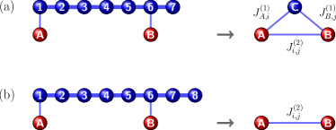
Figure 1: (Color online) Left panel: Two external qubits $A$ and $B$ (red circles) are weakly coupled to an (a) odd-size or (b) even-size spin bus (blue circles). The right-hand panels show the corresponding effective Hamiltonians in the low energy limit. An odd-size spin bus in its ground state acts as an effective spin-$1/2$ particle denoted by $C$. It is coupled to the external qubits with strength $J^{(1)}_{\alpha i}$ at first order in the perturbation theory, and induces an RKKY-like coupling $J^{(2)}_{i,j}$ between the external qubits at second order. The even-size spin bus only mediates an RKKY-like coupling between the external qubits at second order.

The system we consider has two spin qubits $A$ and $B$ weakly attached to an open spin chain $C$, as illustrated in Fig. 1. The Hamiltonian of the total system Friesen07 ; Oh10 ; Shim11 is

$$H=H_{C}+H_{QC}+H_{Q}\,.$$ (1)

In the ideal case with uniform exchange couplings and a uniform external magnetic field (along the $z$ direction, ${\bf B}_{0}=B_{0}\,{\bf\hat{z}}$), the Heisenberg Hamiltonian $H_{C}$ of the spin-$1/2$ chain is written as

$$H_{C}=J_{0}\sum_{i=1}^{N-1}{\mathbf{s}}_{i}\cdot{\mathbf{s}}_{i+1}-g\mu_{B}B_{0}\sum_{i=1}^{N}s_{iz}\,,$$ (2)

where ${\mathbf{s}}_{i}$ is the spin operator of the $i$-th node of the chain, $N$ is the total number of spins in the chain, and $J_{0}>0$ indicates a uniform antiferromagnetic coupling between any two nearest neighbor spins at sites $i$ and $i+1$. In this work, we will assume that a small or vanishing external magnetic field $B_{0}$ is applied to the spin chain (The operation of a spin chain under a finite external magnetic field is discussed in Refs. Shim11, and Shim12, .). Hereafter, the spin chain $C$ will be referred to as a spin bus because it acts as a quantum data bus.

The Hamiltonian $H_{QC}$ describes antiferromagnetic couplings of qubits $A$ and $B$ to the $i$-th spin and the $j$-th spin of the chain, respectively

$$H_{QC}=J_{A,i}\,{\mathbf{s}}_{i}\cdot{\bf S}_{A}+J_{B,j}\,{\mathbf{s}}_{j}\cdot{\bf S}_{A}\,.$$ (3)

We assume that the bus-qubit couplings $J_{\alpha,i}$ with $\alpha=A,B$ are small enough that the spin bus remains in its ground state manifold at all times. In this limit, the total Hamiltonian $H$ can be split into the unperturbed Hamiltonian $H_{0}=H_{C}+H_{Q}$ and the perturbation $H_{1}=H_{QC}$. The perturbation condition is

$$J_{\alpha,i}/\Delta\sim NJ_{\alpha,i}/\pi^{2}J_{0}\ll 1\,,$$ (4)

where $\Delta\sim\pi^{2}J_{0}/N$ is the zero-field gap Lieb61 above the ground state manifold (for an odd-size bus) or ground state (for an even-size bus). $J_{\alpha,i}/\Delta$ is thus used as a perturbation parameter. The qubit-bus coupling $J_{\alpha,i}$ can be turned on and off (gradually), unlike the static intra-bus coupling $J_{0}$. In general, external magnetic fields ${\bf B}_{A}$ and ${\bf B}_{B}$ may be applied to qubits $A$ and $B$ to implement single-qubit operations on them, so that the Hamiltonian $H_{Q}$ can be written as

$$H_{Q}=-g\mu_{B}{\bf B}_{A}\cdot{\bf S}_{A}-g\mu_{B}{\bf B}_{B}\cdot{\bf S}_{B}\,.$$ (5)

There is no direct exchange coupling between qubits $A$ and $B$, as they are nominally well separated. As shown later, the spin bus $C$ can mediate an effective coupling between them if they are both coupled to the bus. Since single-qubit operations are generally done separately from two- or multi-qubit operations, we set $H_{Q}=0$ throughout this paper and will focus on qubit-bus and two-qubit couplings. Note that we will set $\hbar=1$ and $J_{0}=1$ below for convenience.

In the perturbative limit described by Eq. (4), we can perform a canonical transformation of the full Hamiltonian in Eq. (1) to obtain an effective Hamiltonian where the spin bus is in its ground state manifold. Details of the transformation are provided in Appendix A, as well as Refs. Shim11, and Oh11, . The actual form of the effective interaction depends on the parity of the bus. An odd-size spin bus has a doubly degenerate ground manifold, and acts as an effective spin-1/2 particle. At first order in the perturbation theory, the spin-1/2 bus couples directly to the external qubits. At second order, the spin bus mediates an effective RKKY-like coupling between the qubits. The resulting effective Hamiltonian is given as follows: Friesen07 ; Oh10 ; Oh11 ; Shim11

$$H_{\rm eff}^{(2)}=J^{(1)}_{A,i}\,{\bf S}_{A}\cdot{\bf S}_{C}+J^{(1)}_{B,j}\,{\bf S}_{B}\cdot{\bf S}_{C}+J^{(2)}_{i,j}\,{\bf S}_{A}\cdot{\bf S}_{B}\,,$$ (6)

where ${\bf S}_{C}$ is a spin operator representing the ground doublet states of the spin bus. The effective coupling between qubit $\alpha$ and the spin-bus $C$ is given to first order in the perturbation parameter by

$$J_{\alpha,i}^{(1)} \equiv J_{\alpha,i}\,m_{i}\,,$$ (7a)

$$m_{i} =\langle{0;\tfrac{1}{2}}|\sigma_{iz}|{0;\tfrac{1}{2}}\rangle=-\langle{0;-\tfrac{1}{2}}|\sigma_{iz}|{0;-\tfrac{1}{2}}\rangle$$

$$=\langle{0;\tfrac{1}{2}}|\sigma_{ix}|{0;-\tfrac{1}{2}}\rangle\,.$$ (7b)

This is a product of the bare coupling $J_{\alpha,i}$ between the $i$-th spin of the spin bus and the external qubit $\alpha$ and the expectation value $m_{i}$ of $\sigma_{iz}$ at site $i$ in the ground state of the spin bus. Notice that although $m_{i}$ is dimensionless, it can be considered as the local magnetic moment at site $i$ when multiplied by $g\mu_{B}/2$. The RKKY-like second-order coupling $J^{(2)}$ is given by RKKY

$$J^{(2)}_{i,j}\equiv\frac{J_{A,i}J_{B,j}}{2}\sideset{}{{}^{\prime}}{\sum}_{n}\frac{\langle{0}|\sigma_{i\mu}|{n}\rangle\langle{n}|\sigma_{j\mu}|{0}\rangle}{E_{0}-E_{n}}\,.$$ (8)

Here $E_{n}$ and $|{n}\rangle$ are the eigenenergies and eigenstates of $H_{C}$ of an isolated spin bus, and $\sigma_{i\mu}$ with $\mu=x,y,z$ stand for Pauli operators of the $i$-th spin of the spin chain. The prime symbol on the summation indicates the exclusion of the ground states. At zero external field, the ground state $|{0}\rangle$ in Eq. (8) can be either $|{0;\tfrac{1}{2}}\rangle$ or $|{0;-\tfrac{1}{2}}\rangle$, or any linear combination between them. The choice does not change the value of $J^{(2)}_{i,j}$. At a finite magnetic field, however, if the ground state of the spin bus is degenerate, the two states are generally not spin-flipped image of each other. In this case, Eq. (8) has to be modified.

The effective Hamiltonian (6) shows that the odd-size bus at zero or low field acts as an effective spin-$1/2$ particle that is coupled to the external qubits $A$ and $B$, as illustrated in Fig. 1. Although in general $J^{(1)}_{\alpha,i}\gg J^{(2)}_{i,j}$, the second order term plays an essential role in long-time evolutions, such as in quantum state transfer. Oh11 Thus our calculations in the rest of this paper are mostly concerned with these two coupling strengths. Furthermore, we focus on their normalized form $m_{i}=J^{(1)}_{\alpha,i}/J_{\alpha,i}$ and $K_{i,j}\equiv J^{(2)}_{i,j}J_{0}/J_{A,i}J_{B,j}$, which depend only on the size $N$ of the spin bus and the external magnetic field.

For an even-size bus, the sub-Hilbert space of interest is spanned by the non-degenerate ground state of the bus and the four eigenstates of the two qubits (again we focus on the low-field limit). Within this space the bus does not have any dynamics as it is represented by a single ground state. As for the two qubits, there is no first order effective coupling between them here, in contrast to the case of an odd-size bus. The second-order qubit coupling term is obtained in the same way as for an odd-size bus. The effective Hamiltonian to second order in the perturbation is given by Oh10

$$H_{\rm eff}^{(2)}=J^{(2)}_{i,j}\,{\bf S}_{A}\cdot{\bf S}_{B}\,,$$ (9)

where the RKKY-like coupling $J^{(2)}_{i,j}$ has the same form as Eq. (8). In this case, the prime indicates that the non-degenerate ground state is excluded from the summation.

Based on the effective Hamiltonians and the corresponding parameters, we can make some qualitative observations on where the bus-qubit system might be susceptible to randomness and fluctuations. In the case of an odd-size spin bus with attached qubits, the key features that determine the operation of the bus include the Zeeman splitting of the ground doublet of the spin bus, and the energy gap separating the ground doublet and the excited states, $\Delta_{12}$. The former depends on the magnetic environment for the bus, while the latter depends on the interaction strength between the bus nodes. Both the qubit-bus couplings $J^{(1)}_{\alpha,i}$ and the effective qubit-qubit couplings $J^{(2)}_{i,j}$ depend on the local exchange couplings and the local magnetic moments of the bus in its ground state manifold, which is a function of both magnetic environment and the intra-bus exchange couplings. In the case of an even-bus with attached qubits, $J^{(2)}_{i,j}$ has similar dependence on system environment as in the odd-size bus case, and is thus susceptible to variations in both the local magnetic fields and exchange couplings.

III Effects of Randomness

In Sec. II, we have shown how a Heisenberg spin chain with uniform exchange coupling $J_{0}$ acts as a spin bus. Now we address the main question of the present paper, on how static randomness in exchange couplings and external magnetic fields can affect the fitness of the spin chain as a quantum data bus. More specifically, we investigate how such randomness influences the two energy gaps, $\Delta_{01}$ and $\Delta_{12}$, and the effective qubit-bus and qubit-qubit couplings $J^{(1)}_{\alpha,i}$ and $J^{(2)}_{i,j}$.

In order to take into account the effects of randomness in exchange couplings and applied magnetic fields, the Hamiltonian of the chain (2) is generalized to

$$H_{C}=\sum_{i=1}^{N-1}J_{i}\,{\mathbf{s}}_{i}\cdot{\mathbf{s}}_{i+1}-g\mu_{B}\sum_{i=1}^{N}B_{i}\,s_{iz}\,,$$ (10)

where $J_{i}>0$ is the antiferromagnetic coupling between two neighboring spins at sites $i$ and $i+1$, and $B_{i}$ is the local magnetic field at the $i$th site of the spin bus. Note that in spite of the random $J_{i}$ and $B_{i}$, it can be easily shown that Hamiltonian ( 10) still commutes with the $z$ component of the total spin ${\bf S}$, i.e., $[H_{C},S_{z}]=0$.

Hamiltonian (10) may be considered as a finite quantum spin glass model. Das There are several spin glass models depending on the types of couplings (Ising or Heisenberg, and short range or long range) and the distributions of $J_{i}$. For example, the Sherrington-Kirkpatrick model SK75 has the couplings between arbitrary pairs, sampled from the normal distribution with zero mean, while the Edwards-Anderson model EA75 has only the nearest neighbor couplings. In the context of quantum information processing, we can reasonably assume that the exchange couplings and the applied magnetic fields are both near their target values, $J_{0}$ and $B_{0}$. The random exchange couplings $J_{i}$ and applied magnetic fields $B_{i}$ are then

$$J_{i} =J_{0}+\delta J_{i}\,,$$ (11a)

$$B_{i} =B_{0}+\delta B_{i}\,.$$ (11b)

In the numerical analysis described below, we choose $\delta J_{i}$ and $\delta B_{i}$ that are randomly sampled from normal distributions with standard deviations $\sigma_{J}$ and $\sigma_{B}$, respectively. In experimental systems, we would expect such variations to be small, assuming reasonable calibration efforts. In the following studies, we analyze these two types of random variations separately, keeping one of the variables uniform.

III.1 Effects of Random Exchange Couplings in Odd-size Buses

In this subsection, we investigate how random variations in the inter-node exchange couplings $J_{i}$, given by Eq. (11a), affect the ability of an odd-size chain to function as a spin bus. Such variations could result from calibration errors, slow but random hopping of charge traps near the spin bus nodes, and whatever other factors that are not accounted for during the calibration process. Here the external magnetic field $B_{0}$ on the chain is set to be zero or small, so that the system remains in the isotropic regime. The external magnetic field, if any, is taken to be uniform, so that $\delta B_{i}=0$.

The variations $\delta J_{i}$ are small compared to $J_{0}$, so that they may be treated as a perturbation:

$$H_{C} =H_{C}^{(0)}+V\,,$$ (12a)

where $$H_{C}^{(0)} V$$ is the unperturbed Hamiltonian (2), and the perturbation is given by

$$V=\sum_{i=1}^{N-1}\delta J_{i}\,{\mathbf{s}}_{i}\cdot{\mathbf{s}}_{i+1}\,.$$ (12b)

Hereafter the superscript ⁽⁰⁾ is used to denote the case of uniform exchange coupling or uniform magnetic fields in the bus.

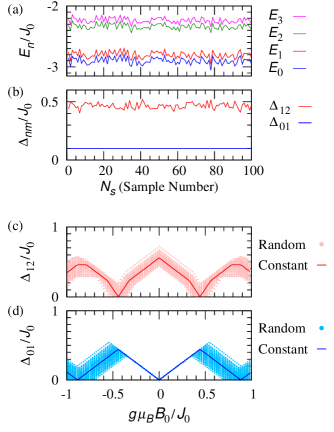
Figure 2: (Color online) (a) Four lowest energy levels, $E_{0},E_{1},E_{2}$ and $E_{3}$, and (b) two energy gaps, $\Delta_{01}=E_{1}-E_{0}$ and $\Delta_{12}=E_{2}-E_{1}$ are plotted as a function of sample number $N_{S}$ of odd-size chains with size $N=7$ with random exchange couplings $J_{i}$ with the standard deviation $\sigma_{J}/J_{0}=0.1$ at $g\mu_{B}B_{0}/J_{0}=0.1$. In (c) and (d), two energy gaps $\Delta_{01}$ and $\Delta_{12}$ are plotted as a function of $B_{0}$ for the samples $N_{s}=100$.

Here we consider an ensemble of $N_{S}$ odd-size chains. Each of the samples in this ensemble has the same size $N$ but different $J_{i}$ sampled from the normal distribution with average $J_{0}$ and standard deviation $\sigma_{J}$. Fig. 2(a) shows the fluctuations in energy levels as a function of sample number, at a low magnetic field of $g\mu_{B}B_{0}/J_{0}=0.1$. The two lowest energy levels $E_{0}$ and $E_{1}$ fluctuate in sync, so that the gap $\Delta_{01}$ is free from the randomness of $J_{i}$ [shown in Fig. 2(b)]. The energies $E_{2}$ and $E_{3}$ of $|2\rangle$ and $|3\rangle$ are also in sync, as shown in Fig. 2 (a). However, the gap $\Delta_{12}$, which is a measure of the isolation of the ground doublet from the excited states, does fluctuate [as shown in Fig. 2(b)], because $E_{1}$ and $E_{2}$ have different dependence on the exchange coupling. In other words, while the ground state splitting $\Delta_{01}$ of this odd-size bus is robust against the randomness in exchange coupling, the ground-excited-state gap $\Delta_{12}$ is affected by the randomness. In Figs. 2 (c) and (d) the two gaps, $\Delta_{01}$ and $\Delta_{12}$, are plotted as a function of the uniform magnetic field $B_{0}$ applied on the bus. At low fields, the ground state gap $\Delta_{01}$ increases linearly and without broadening as the magnetic field increases, until $g\mu_{B}B_{0}/J_{0}\sim 0.35$. It starts to be influenced by the exchange randomness above $g\mu_{B}B_{0}/J_{0}\sim 0.35$, which corresponds to the crossing between levels $|{2}\rangle$ and $|{3}\rangle$, as shown in Fig. 14 in Appendix A.1. Beyond this crossing point, states $|1\rangle$ and $|0\rangle$ are not the time-reversal of each other anymore due to the level crossings with higher excited states. Recall that for a spin chain to act as a spin bus, we need the ground state doublet to be well separated from the excited states, or $\Delta_{12}\gg\Delta_{01}$. Panels (c) and (d) of Fig. 2 indicate that this condition is satisfied when the bus ground doublet is energetically separated from excited states ($g\mu_{B}B_{0}/J_{0}\lesssim 0.2$), and acts as an effective spin-1/2 system with a constant magnetic moment.

Although $[H_{C},S_{z}]=0$ dictates that the dimensionless total magnetic moment $\sum_{i}m_{i}=\pm 1$ of the ground state is still a good quantum number despite random exchange couplings, the local magnetic moment $m_{i}$ does fluctuate around $m_{i}^{(0)}$, as shown in Fig 3. Consequently, the first-order effective coupling $J_{\alpha,i}^{(1)}$ between the qubit and the bus, given by Eq. (7), is affected by the randomness in the bus exchange coupling, and has to be calibrated individually.

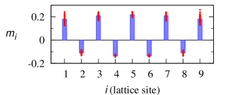
Figure 3: (Color online) Dimensionless local magnetic moments $m_{i}=\langle{0;\tfrac{1}{2}}|\sigma_{iz}|{0;\tfrac{1}{2}}\rangle$ are plotted (red dots) for all lattice sites on an odd-size spin bus with $N=9$ for an ensemble of $N_{S}=100$ random samples, with $\sigma_{J}/J_{0}=0.01$ and $B_{0}=0$. The height of the blue bars represents the local magnetic moment $m_{i}^{(0)}$ for uniform exchange couplings ($\delta J=0$). The spread of the red dots at each bus node illustrates the variations in local magnetic moments due to the random exchange couplings, with larger variations apparent at the end sites.

The effective qubit-qubit coupling $J^{(2)}_{i,j}$ is also affected by the randomness of the intra-bus exchange couplings $J_{i}$. As indicated in Eq. (8), $J^{(2)}_{i,j}$ is determined by the full bus spectrum, including both the energy levels and the excited states. Figures 2 and 3 show that the random exchange couplings $J_{i}$ in general affect the energy gaps from the ground state, $E_{n}-E_{0}$, as well as the bus eigenstates $|{n}\rangle$. Thus we expect that $J^{(2)}_{i,j}$ should be sensitive to the randomness in $J_{i}$. Figure 4 shows how the ensemble averages of the gap, $\langle\Delta_{01}\rangle_{\rm en}$, the local magnetic moment, $\langle m_{5}\rangle_{\rm en}$ (which is the normalized first-order qubit-bus coupling $J^{(1)}_{A,5}/J_{A,5}$), and the normalized second-order effective coupling, $\langle K_{i,j}\rangle_{\rm en}=\langle J^{(2)}_{i,j}\rangle_{\rm en}\,{J_{0}}/{(J_{A,1}J_{B,5})}$ depend on the fluctuations of the exchange coupling, represented by the standard deviation $\sigma_{J}$, over a 5-node bus. The blue filled circles in Fig. 4 show how the fluctuations in these quantities depend on the randomness in the exchange couplings. For example, when $\sigma_{J}/J_{0}=0.1$, $\sigma(m_{5})\sim\sigma(K_{1,5})\sim\frac{1}{6}$, which indicates that the effective qubit-bus coupling and the effective qubit-qubit coupling have similar sensitivities to the random variations in the intra-bus exchange couplings.

Furthermore, both the local magnetic moment (thus the qubit-bus coupling) and the effective qubit coupling are linear functions of $\sigma_{J}$, with their slopes depending on the size of the bus. These slopes are indicators of sensitivity of $J^{(1)}$ and $J^{(2)}$ to the exchange variations, and can be used in evaluating decoherence in such a spin bus architecture. For example, background charge fluctuations can affect exchange couplings between neighboring nodes of a spin bus. As a result, the effective qubit-qubit exchange coupling becomes a time-dependent random variable, which leads to two-qubit dephasing. HuPRL06 The relevant correlation function that determines the dephasing is $\langle J^{(2)}(t)J^{(2)}(0)\rangle$, and is given approximately by $\left[\sigma(J^{(2)})/\sigma_{J}\right]^{2}{\langle J_{i}(t)J_{i}(0)\rangle}$ HuPRL06 . The latter correlation function, $\langle J_{i}(t)J_{i}(0)\rangle$, represents fluctuations in the individual inter-node exchange couplings along the bus, whose dynamics is determined by the environmental charge noise.

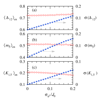
Figure 4: (Color online) For odd-size chain with $N=5$, the ensemble averages of (a) the gap $\langle\Delta_{01}\rangle_{\rm en}$ in units of $J_{0}$, (b) the dimensionless local magnetic moment $\langle m_{5}\rangle_{\rm en}$ at the end of the chain, and (c) the normalized second-order effective coupling $\langle K_{i,j}\rangle_{\rm en}=\langle J^{(2)}_{1,5}\rangle_{\rm en}J_{0}/(J_{A,1}J_{B,5})$ are plotted (open red circle) as a function of the standard deviation $\sigma_{J}$ of $\delta J_{i}$. The blue filled circles in each panel indicate the standard deviations of each data point, which is obtained by averaging over 2000 random configurations. Here $B_{0}=0$.

In summary, even when intra-bus exchange couplings of an odd-size spin chain have random but static variations, the chain can still act as a spin bus, with a ground state doublet that is well separated from the excited states, and acts as an effective spin-1/2 system with a constant magnetic moment. However, the effective qubit-bus couplings and the mediated qubit-qubit couplings are affected by the randomness in exchange, with their fluctuations linearly proportional to the randomness in exchange. Calibration would thus be needed for accurate qubit operations. The results here also have implications for spin-bus related decoherence. In essence, the strong exchange couplings allow a spin bus to process quantum information across a large distance, but also make the qubit-bus system susceptible to charge noise via both $J^{(1)}_{i,\alpha}$ and $J^{(2)}_{i,j}$.

III.2 Effects of Random Magnetic Fields in Odd-size Buses

Spin qubits are generally susceptible to magnetic noise, and the spin bus is no exception. Here we examine how random but static external magnetic fields affect the properties of an odd-size spin bus. Our results should also be a useful indicator of the sensitivity of a spin bus to temporal magnetic noise, as we will discuss later in the section. For this calculation we assume that the exchange couplings $J_{i}$ are uniform, and focus on the magnetic randomness.

The local magnetic fields, Eq. (11b), are

$$B_{i}=B_{0}+\delta B_{i}\,,$$ (13)

where the random field $\delta B_{i}$ is sampled from a normal distribution with standard deviation $\sigma_{B}$. As in the previous subsection, we consider an ensemble of $N_{S}$ spin chains, so that the ensemble average of local magnetic field $B_{i}$ is $\langle{B_{i}}\rangle_{\rm en}=B_{0}$ and $\langle{\delta B_{i}}\rangle_{\rm en}=0$ in the limit of large $N_{S}$. Such a random distribution of local magnetic field could originate from quasi-static nuclear hyperfine fields, or local paramagnetic centers in a semiconductor.

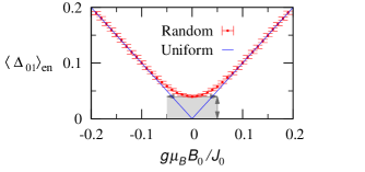
Figure 5: (Color online) Ensemble average of the gap $\langle{\Delta_{01}}\rangle_{\rm en}$ in units of $J_{0}$ between the two lowest states of a single spin as a function of the external magnetic field $B_{0}$. The height and the width of the rectangle, touching the bottom of the curve, indicates $g\mu_{B}\sigma_{B}/J_{0}$ and $\langle{\Delta_{01}}\rangle_{\rm en}/J_{0}$ at $B_{0}=0$, respectively.

As a benchmark, we first recall how an odd-size spin chain behaves in a constant uniform magnetic field. When $B_{0}=0$, the odd-size chain has two doubly degenerate ground states with the total magnetic moment $S_{z}=\pm 1/2$. A finite $B_{0}$ splits these two states like a single spin-$1/2$ particle. There are two important features that determine the behavior of the ground doublet in a magnetic field: the energy splitting $\Delta_{01}$, and the ground state spin orientation. In a uniform field the latter depends only on the $g$-factor of the material, while in a random field it also depends on the local field configuration.

We first examine how the random external magnetic field affects $\Delta_{01}$, the splitting of the ground state doublet of the odd-size bus. This dependence is a good indicator of whether the ground state doublet of an odd-size spin bus is a robust effective spin-1/2. Note that the commutation relation $[H_{C},S_{z}]=0$ holds even in a random magnetic field, so the two lowest states have $S_{z}=\pm 1/2$ (recall that the inter-node coupling is anti-ferromagnetic). Figure 5 shows that the randomness in the magnetic field induces a finite average gap at zero field. This gap opens at $B_{0}=0$ even though $\langle{\delta B_{i}}\rangle_{\rm en}=0$. This non-vanishing average gap between the two lowest states is a consequence of the statistical behavior of the random field, and can be understood using a model of $N_{S}$ single spins in a Gaussian ensemble of random external magnetic fields $\delta B$ with $B_{0}=0$. The Hamiltonian of a single spin is

$$H=-g\mu_{B}\,\delta B\,\frac{\sigma_{z}}{2}\,.$$ (14)

The energy splitting of each spin is given by $\Delta_{01}=g\mu_{B}|\delta B|$, which is always positive. It is thus not a surprise that the ensemble average of the gaps, $\langle{\Delta_{01}}\rangle_{\rm en}=g\mu_{B}\langle{|\delta B|}\rangle_{\rm en}$, is nonzero, even though $\langle{\delta B}\rangle_{\rm en}=0$—the ground state changes according to the field configuration.

To make this argument more rigorous, recall that for a normal distribution, the odd central absolute moments of a random variable $X$ with a mean of $\mu$ are given by

$${\mathbb{E}}\left(|X-\mu|^{p}\right)=\frac{\sigma^{p}(1-p)!!}{\sqrt{2\pi}}\,,$$ (15)

where $!!$ denotes the double factorial. Applying Eq. (15) to $\Delta_{01}$, we get

$$\langle{\Delta_{01}}\rangle_{\rm en}=g\mu_{B}\frac{\sigma_{B}}{\sqrt{2\pi}}\,,$$ (16)

where $\sigma_{B}$ is the standard deviation of $\delta B$. While in our case the magnetic moment of the ground state is distributed throughout the whole spin chain, its splitting is still mainly due to the Zeeman splitting of a single Bohr magneton, so that the single-spin argument provided here is still applicable. When $B_{0}\neq 0$, the average gap can be qualitatively expressed as $\langle{\Delta_{01}}\rangle_{\rm en}\propto g\mu_{B}\sqrt{\langle{(B_{0}+\delta B)^{2}}\rangle}\sim g\mu_{B}\sqrt{B_{0}^{2}+\sigma_{B}^{2}}$, which is a hyperbola that saturates at $B_{0}=0$ to $g\mu_{B}\sigma_{B}$ and approaches $g\mu_{B}B_{0}$ at large $B_{0}$. The difference in the proportionality constant originates from the difference between $\langle{|f|}\rangle$ and $\sqrt{\langle{f^{2}}\rangle}$.

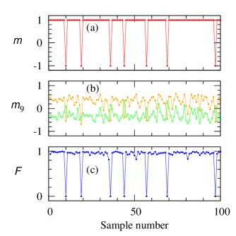
Figure 6: (Color online) (a) Total magnetic moment $m$ of the ground state $|{0}\rangle$, (b) local magnetic moment $m_{9}$ for the ground state $|{0}\rangle$ (orange solid circle) and for the first excited state $|{1}\rangle$ (green open circle), and (c) the fidelity $F$ of the ground state in the presence of random magnetic fields with respect to that in the uniform field as a function of the sample number. Here the size of spin buses is $N=9$, $g\mu_{B}B_{0}/J_{0}=0.1$, and $g\mu_{B}\sigma_{B}/J_{0}=0.065$.

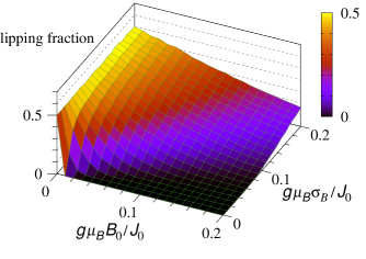
Figure 7: (Color online) The fraction of flipped ground states for $N_{s}=10000$ random realizations of odd-size chains with $N=5$, as a function of $B_{0}$ and $\sigma_{B}$.

Now we address the spin orientation of the odd-size spin bus in the ground state under random magnetic fields. The magnetic moment of a single spin (with $g=2$) in the ground state is anti-parallel to the external field. As in the single spin case, the total magnetic moment of the odd-size spin bus in the ground state is always anti-parallel to a small uniform external magnetic field. As shown in Fig. 3, the local magnetic moments align antiferromagnetically (alternation between anti-parallel and parallel alignments). Even in a random external magnetic field in the $z$-direction, the two lowest states of an odd-size spin bus are characterized by $S_{z}=1/2$ or $S_{z}=-1/2$, so one might guess the Zeeman energy would determine the spin orientation. However, this is not the case.

Figure 6 shows the total magnetic moment of the ground state $|{0}\rangle$ in an ensemble of random magnetic fields for the case when $N=9$ and $\sigma_{B}/B_{0}=0.65$. As illustrated in panels (a) and (c), seven samples, #10, #19, #36, #44, #57, #69, and #97, among 100 samples have negative total magnetic moment $m=-1$, so that their ground state is $|{n=0;S_{z}=-\tfrac{1}{2}}\rangle$ instead of $|{n=0;S_{z}=\tfrac{1}{2}}\rangle$. Panel (b) of Fig. 6 shows a strongly random local magnetic moment on the 9-node spin bus, with the seven flipped states having reversed local magnetic moments. The probability for either $|{n=0;S_{z}=-\tfrac{1}{2}}\rangle$ or $|{n=0;S_{z}=\tfrac{1}{2}}\rangle$ to be the ground state depends on the ratio of $B_{0}$ and $\sigma_{B}$, as illustrated in Fig. 7. As expected, when $B_{0}=0$, the probability is 50%. A strong uniform field $B_{0}$ (compared to $\sigma_{B}$) suppresses the flipping fraction and stabilizes one of the states as the predominant ground state.

A close inspection of the data presented in Fig. 6 reveals that Zeeman splitting of the local nodes of a spin bus does not tell the whole story of $\Delta_{10}$, so that the single-spin model has its limitations. By definition, the energy gap is

$$\Delta_{10}=E_{1}-E_{0} = \langle{1}|H_{J}|{1}\rangle-\langle{0}|H_{J}|{0}\rangle$$ (17)

$$-\mu_{B}\sum_{i}B_{i}(\,m_{i}^{1}-m_{i}^{0}\,)$$

$$= E_{J}^{1}-E_{J}^{0}+E_{Z}^{1}-E_{Z}^{0}\,.$$

Here $H_{J}$ and $H_{Z}$ represent the exchange and Zeeman components of $H_{C}$ in Eq. (10), $E_{Z}^{k}=\langle{k}|H_{Z}|{k}\rangle=-\mu_{B}\sum_{i}B_{i}m_{i}^{k}$ and $E_{J}^{k}=\langle{k}|H_{J}|{k}\rangle$ denote the Zeeman and exchange contributions to the energy of state $|{k}\rangle$, with $k=0,1$, $m_{i}^{k}\equiv\langle{k}|\sigma_{iz}|{k}\rangle$ is the local magnetic moment at bus node $i$, and we have taken $g=2$ for simplicity. When the external magnetic field is uniform, $B_{i}=B_{0}$, the exchange contribution to the energy of $|{0}\rangle$ and $|{1}\rangle$ in Eq. (17) are the same, so that $E_{J}^{1}-E_{J}^{0}=0$, and $m_{i}^{0}$ are equal in magnitude and opposite in sign to $m_{i}^{1}$. Thus the gap between the two states is given completely by the Zeeman splitting: $E_{1}-E_{0}=2\mu_{B}B\sum_{i}m_{i}^{0}=2\mu_{B}Bm^{0}$. With $g=2$, the net spin of the ground state $|{0}\rangle$ is parallel to the uniform magnetic field ${\bf B}$ like a single spin, so that $|{0;S_{z}=1/2}\rangle$ is the ground state when $B$ is positive.

Under a random magnetic field $B_{i}$, but with $B_{0}\gg\sigma_{B}$, the exchange contribution to the gap in Eq. (17) is still negligible, and the ground state spin is parallel to $B_{0}$. However, if $B_{0}$ is of the order of $\sigma_{B}$ or smaller, the ground state total spin orientation may be anti-parallel rather than parallel to $B_{0}$ . For these configurations with the “flipped” ground state, the reason for the flipping is varied. Consider the samples (from the ensemble of 9-node buses presented in Fig. 6) shown in Fig. 8 and Table 1. Here sample #0 refers to the spin bus in a uniform magnetic field. Samples #6, #10, #19 and #36 are for the bus in different random magnetic field configurations, and the later three samples have a flipped ground state, with $m^{0}=-1$. Figure 8 shows that in a random magnetic field, the local magnetic moments for the two lowest states are generally not equal in magnitude, $|m_{i}^{0}|\neq|m_{i}^{1}|$, so that the two states $|{0}\rangle$ and $|{1}\rangle$ are no-longer spin-flipped image of each other, even though $\sum_{i}m_{i}^{k}=\pm 1$. The most dramatic examples are those samples with a flipped ground state, where the ground and first excited states are far from the classical anti-ferromagnetic spin configurations. This also implies that in general the Zeeman energy $E_{Z}^{0}\neq-E_{Z}^{1}$. Samples #6 and #10 demonstrate that even if all the magnetic fields $B_{i}$ are positive, the ground state could still be either $S_{z}=1/2$ or $S_{z}=-1/2$. While in most cases the energy gap between the two lowest states in Eq. (17) is due to the Zeeman term, for samples #10 and #19 the Zeeman energies $E_{Z}^{0}$ and $E_{Z}^{1}$ are almost equal, so that there is no Zeeman gap. The energy gaps for these two samples are determined by the exchange contribution in Eq. (17), and are one or two orders of magnitude smaller than the usual Zeeman gap. For sample #36, the total energy gap is dominated by the Zeeman contribution (with significant contribution also coming from the exchange interaction), although the configuration of the random magnetic field is such that the ground state is flipped. In short, when $B_{0}\lesssim\sigma_{B}$, the local and total magnetic moments of the ground state are sensitively dependent on the distribution of the random magnetic field.

Sample No.	$E_{1}-E_{0}$	$E_{Z}^{1}-E_{Z}^{0}$	$E_{J}^{1}-E^{0}_{J}$	$\quad|\Delta E_{J}/\Delta E_{Z}|$
#0	0.2	0.2	0.0	0 %
#6	0.27083	0.25840	0.01244	4.8 %
#10	0.00403	-0.00840	0.01243	148.0 %
#19	0.06222	-0.01582	0.07804	493.3 %
#36	0.06989	0.04306	0.02683	62.3 %

Table 1: (Color online) Energy gap $E_{1}-E_{0}$ between the bus states $|{0}\rangle$ and $|{1}\rangle$, its Zeeman contribution $E_{Z}^{1}-E_{Z}^{0}$, the exchange contribution $E_{J}^{1}-E_{J}^{0}$, and the absolute ratio of these contributions for samples #0, #6, #10, #19, and #36 in Fig. 6. Here the energy is measured in units of $J_{0}$.

Our results so far indicate that random magnetic fields can seriously undermine the capabilities of a spin bus, by altering the local magnetic moments (and thus the effective qubit-bus coupling $J^{(1)}$) and the bus ground state. Fortunately, in general $\sigma_{B}$ is relatively small. For example, if the random field is due to hyperfine interaction in GaAs, $\sigma_{B}\sim 2$ mT for a 100 nm quantum dot, so that a $B_{0}>20$ mT should be more than enough to overcome the effect of the random field. Furthermore, the above discussion is applicable to the regime where the magnetic energy scales are not much smaller than the exchange energy scales (e.g., for Fig. 6 and Table 1, $\mu_{B}\sigma_{B}/J_{0}=0.0650$). If $J_{0}\gg B_{0}$ and $\sigma_{B}$, the structures of the ground and first excited states of the spin chain should be determined by the anti-ferromagnetic coupling and are less susceptible to the small magnetic field or its fluctuations. In this case the ground state spin orientation would be mostly determined by the Zeeman contribution to the energies of the two states, and we would recover the simple single-spin physical picture.

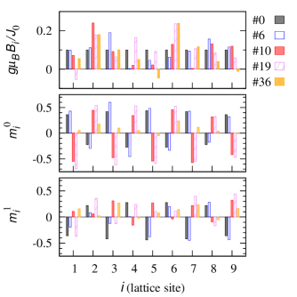
Figure 8: (Color online) Local magnetic moments of the ground and first excited states for several random field configurations in a 9-node spin bus. Here sample #0 corresponds to the case of a uniform applied field. The others correspond to the samples in Fig. 6. The total magnetic moment of the ground states of samples #0 and #6 is $m^{0}=1$, i.e., $S_{z}=1/2$. On the other hand, samples #10, #19, and #36 have the spin-flipped ground states, $m^{0}=-1$, i.e., $S_{z}=-1/2$.

The fluctuations in the local magnetic moments of the spin bus due to the random external magnetic field lead directly to fluctuations in the effective qubit-bus couplings $J^{(1)}_{i,\alpha}$ [see Eq. (7)], though this fluctuation is suppressed if $B_{0}\gg\sigma_{B}$, as illustrated by the few data points for small $\sigma_{B}/B_{0}$ in Panel (b) of Fig. 9. In addition, under a random magnetic field, the effective coupling $J_{\alpha,i}^{(1)}$, given by Eq. (7), becomes anisotropic. This is in addition to the anisotropy induced by a finite $B_{0}$.Shim12 In general, anisotropy occurs when

$$\langle{0}|\sigma_{ix}|{1}\rangle \neq\frac{1}{2}\Bigl{[}\,\langle{0}|\sigma_{iz}|{0}\rangle-\langle{1}|\sigma_{iz}|{1}\rangle\,\Bigr{]}\,,$$ (18a)

and

$$\sum_{i=1}^{N} \langle{0}|\sigma_{ix}|{1}\rangle\neq 1\,.$$ (18b)

The anisotropy appears in both $J^{(1)}$ and $J^{(2)}$ Shim11 , as illustrated in Panels (b) and (c) of Fig. 9. Based on the standard deviation data presented in panel (b), we also observe that while the transverse component of the local magnetic moment is reasonably robust against the randomness in the magnetic field, the longitudinal component is not. On the other hand, panel (c) shows that both the longitudinal and transverse components of the effective qubit-qubit coupling $J^{(2)}$ have a linear dependence on the field randomness for small $\sigma_{B}$, changing to a different slope as $\sigma_{B}$ becomes larger than $B_{0}$. Both of these observations illustrate the fact that for an odd-size spin bus to function properly, magnetic field randomness in the system needs to be minimized.

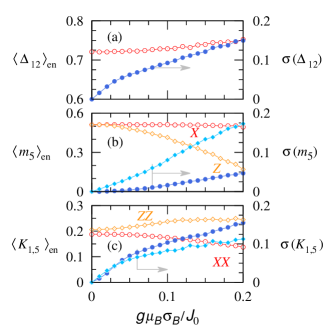
Figure 9: (Color online) For an odd-size spin bus with $N=5$, the ensemble averages of (a) the gap $\langle\Delta_{12}\rangle_{\rm en}$ in units of $J_{0}$, (b) the local magnetic moment $\langle m_{5}\rangle_{\rm en}$ on one end of the chain, and (c) the normalized second-order effective coupling $\langle K_{1,5}\rangle_{\rm en}$ are plotted as a function of the standard deviation $\sigma_{B}$ of $\delta B_{i}$. In (b), the labels “X” (symbol: red open circle) and “Z” (symbol: orange open diamond) stand for the $x$- and $z$- components of the first-order effective coupling, respectively. In (c) the labels “XX” (symbol: red open circle) and “ZZ” (symbol: orange open diamond) refer to the $xx$- and $zz$-component of the second-order effective coupling, respectively. Here $\mu_{B}B_{0}/J_{0}=0.05$. In panels (b) and (c), the solid diamonds and solid circles represent standard deviations for the data labeled by the open diamonds and open circles, respectively.

As explained in Sec. II, the effective qubit-qubit coupling $J^{(2)}$ given by Eq. (8) is well defined when the degenerate or nearly degenerate ground states of the spin bus are spin-flipped states of each other. This is the case for an odd-size spin bus near zero external magnetic field. At certain finite external fields, the ground states of the spin bus would be close to be degenerate again. However, in those regimes Eq. (8) is generally not applicable and should be modified. Shim12

In summary, the effects of the random magnetic field in the $z$-direction on an odd-size bus are as follows. First, the degeneracy in the ground states of an odd-size bus is lifted. Second, although the two lowest states have either $S_{z}=1/2$ or $S_{z}=-1/2$, the spin orientation of the ground state is not solely determined by the Zeeman energy. Third, the random magnetic fields make the first-order and the second-order effective couplings anisotropic.

III.3 Effects of Random Exchange Couplings in Even-size Buses

In this subsection, we investigate how an even-size spin bus is affected by random exchange couplings $J_{i}$. Recall that the effective Hamiltonian for an even-size bus coupled to two qubits in zero magnetic field takes the form of $H_{\rm eff}^{(2)}=J^{(2)}_{i,j}\,{\bf S}_{A}\cdot{\bf S}_{B}$, where $J^{(2)}_{i,j}$ is given by Eq. (8). The various terms in this equation are the bare qubit-bus couplings $J_{A,i}$ and $J_{B,j}$, the bus energy gaps $\Delta_{0n}=E_{n}-E_{0}$, and the transition matrix elements $\langle{0}|\sigma_{i\mu}|{n}\rangle$. Here we examine the effects of random intra-bus exchange couplings on these different terms, with a particular focus on the gap $\Delta_{01}$ between the ground and the first excited state, which is an indicator of how well the nondegenerate ground state is isolated from the excited states, and figures prominently in the expression of $J^{(2)}$.

An even-size bus can be thought of as an odd-size bus plus an extra spin-1/2 node. Thus the lowest four states of an even-size bus is a singlet and a triplet. A uniform magnetic field would split the triplet, but would not affect the singlet ground state. With random exchange couplings, similar to the case of an odd-size bus, we still have $[H,S_{z}]=0$, so that the triplet splitting is given by Zeeman splitting. The random exchange couplings do cause the energy levels and the eigenstates to vary in general. For example, Fig. 10 plots the two energy gaps, $\Delta_{01}$ and $\Delta_{12}$, as a function of $B_{0}$ for 100 samples of even-size chains with random exchange couplings. While the ground state remains nondegenerate, the gap $\Delta_{01}$ is now distributed between 0.3 and $0.5\,J_{0}$ at $B_{0}=0$. Around $B_{0}=0$, the gap $\Delta_{12}$ and the next gap $\Delta_{23}=E_{3}-E_{2}$ (not plotted) are robust against the random exchange couplings $J_{i}$, reflecting the fact that these two gaps correspond to the Zeeman splittings of the triplet bus states. This is similar to the $\Delta_{01}$ gap of an odd-size bus near zero field, which corresponds to the Zeeman splitting of the spin-1/2 doublet ground state, as shown in Fig. 2.

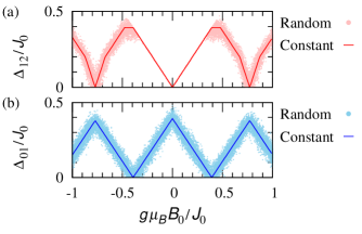
Figure 10: (Color online) For $N_{s}=100$ even-size chains with random exchange couplings, two lowest energy gaps, (a) $\Delta_{12}=E_{2}-E_{1}$ and (b) $\Delta_{01}=E_{1}-E_{0}$, are plotted as functions of $B_{0}$. The size of each chain is $N=8$ and the standard deviation $\sigma_{J}/J_{0}$ of $\delta J_{i}$ is 0.025.

The most important effect of the randomness in the exchange couplings for bus operations is on the low lying energy gaps such as $\Delta_{01}$. As shown in panel (b) of Fig. 11, the ground state itself is quite robust against the random exchange coupling in terms of state fidelity, and has zero local magnetic moments as well as zero total magnetic moment. This is in contrast with the effect of random magnetic fields on the even-size bus as shown in subsection III.4, where the local magnetic moments become non-zero. On the other hand, while the average value of the $\Delta_{01}$ gap is only weakly dependent on $\sigma_{J}$, the fluctuations in $\Delta_{01}$ depend linearly on $\sigma_{J}$, as shown in panel (a) of Fig. 11. Consequently, the fluctuations of the bus-mediated qubit-qubit coupling also has a linear dependence on the standard deviation $\sigma_{J}$ of $\delta J_{i}$, as shown in panel (c) of Fig. 11. The slope $\sigma_{J^{(2)}}/\sigma_{J}$ is quite large here, reflecting a sensitive dependence of the singlet-triplet splitting of the spin bus on the intra-bus exchange couplings. While calibration should be able to largely suppress the effects of any static randomness of the exchange coupling, the sensitivity to randomness in the local exchange, as indicated by the large $\sigma_{J^{(2)}}/\sigma_{J}$, dictates that effects of environmental charge noise on the inter-node exchange coupling $J_{i}$ need to be minimized.

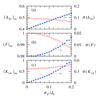
Figure 11: (Color online) For an even-size bus with $N=6$, (a) the ensemble averages of the ground energy gap $\Delta_{01}$, (b) the fidelity $F$ with respect to the uniform ground state, and (c) the normalized effective qubit-qubit coupling $K_{1,6}=J^{(2)}_{1,6}J_{0}/J_{1,A}J_{6,B}$ are plotted as functions of the fluctuation $\sigma_{J}$ of the random exchange coupling (all data are represented by red open circles). Here $B_{0}=0$ and the sample size is $N_{s}=100$. The blue solid circles represent the standard deviation of $\Delta_{01}$, $F$, and $K_{1,6}$, respectively.

III.4 Effects of Random Magnetic Fields in Even-size Buses

In this subsection, we study how an even-size bus is affected by an external magnetic field that has random local variations. In a uniform but small external magnetic field, the ground state of the even-size bus has zero local magnetic moments as well as zero total magnetic moment ($S_{z}=0$). Recall that the commutation relation $[H_{C},S_{z}]=0$ is still valid even when the bus is subject to random magnetic fields $B_{i}$ in the $z$-direction. If the random magnetic fields are weak, the even-size bus remains in the ground state with $S_{z}=0$, i.e., zero total magnetic moment. However, the local magnetic moments $m_{i}$ become non-zero in contrast with the case of a uniform magnetic field. Furthermore, the bus excited states generally do have net magnetic moments, so that they respond to both local and global magnetic fields in terms of their energies and their state composition.

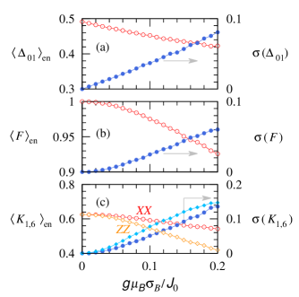
Figure 12: (Color online) Effect of random magnetic field for an even-size bus with $N=6$. (a) The average ground energy gap $\Delta_{01}$ in units of $J_{0}$, (b) the average fidelity $F$ of the ground states with respect to that without random $B_{j}$, and (c) the average of the normalized second-order effective coupling $K_{1,6}$ are plotted (in open red circles or open orange diamonds) as a function of the standard deviation of the random magnetic field $\sigma_{B}$. The standard deviations of the averages are given by the blue solid circles or blue solid diamonds, respectively. Here we take $B_{0}=0$.

In Fig. 12 we plot the effect of the locally random magnetic field on the gap $\Delta_{01}$, the ground state robustness (in terms of the fidelity $F$ with respect to the uniform field ground state), and the bus-mediated qubit-qubit interaction $J^{(2)}_{1,6}$. The average of gap $\Delta_{01}$ decreases with $\sigma_{B}$ because for any particular random field configuration, one of the polarized triplets has a lower energy compared to the zero field case and becomes the first excited state. The linear increase in the standard deviation of $\Delta_{01}$ is simply a reflection of the linear nature of the Zeeman splitting. In panel (b), the decrease in the fidelity shows that the local magnetic moments may fluctuate although their sum, i.e., the total magnetic moment is still zero. Interestingly, in panel (c), the normalized effective coupling $K_{1,6}=J^{(2)}_{1,6}J_{0}/J_{A,1}J_{B,6}$ and its standard deviation both have a super-linear dependence on $\sigma_{J}$ when it is small, making the coupling a robust quantity against field randomness. The qualitative reason for this robustness is that the ground state is not coupled to the two polarized triplet states of the bus by the random magnetic field along $z$ direction at the lowest order, while the gap between the unpolarized triplet state and the ground state only depends on the field randomness quadratically. In this calculation we did not consider a random transverse field since our focus is on static disorder. For example, for magnetic disorder caused by random nuclear polarizations, the transverse polarizations would precess around the external field, so that their effect would tend to be suppressed.

In Ref. Shim11, , we have shown that a constant external magnetic field makes the second-order effective interaction mediated by an even-size bus anisotropic. Here we find that local random variations in the magnetic field, $\delta B_{i}$, also induce anisotropy, even if $B_{0}=0$ and $\langle\delta B_{i}\rangle_{\rm en}=0$, as shown in panel (c) of Fig. 12. This anisotropy is weaker compared to the case of an odd bus in a finite $B_{0}$ as shown in Fig. 9, because the average of the local field here vanishes ($B_{0}=0$), so that the spatial isotropy is not broken as completely as in the case of Fig. 9. Note that we would normally expect an even-size bus to be operated at zero external magnetic field $B_{0}=0$, unless the anisotropy of the effective coupling is desired.

IV Conclusions

We have performed a comprehensive study of the effects of local randomness in the exchange couplings and the external magnetic field on the capabilities of a strongly coupled Heisenberg spin bus.

We find that the random exchange couplings preserve the isotropic symmetry (in the qubit-bus and qubit-qubit couplings) of the bare Heisenberg coupling. This symmetry also makes the ground Zeeman energy gap of the odd-size bus robust against small fluctuations in the exchange couplings. However, randomness in the exchange couplings does cause the eigenenergies and the eigenstates to vary, which in turn leads to randomness in the magnitudes of the effective couplings (both qubit-bus and qubit-qubit).

An external magnetic field, whether uniform or random, does break the isotropy of the Heisenberg spin bus, and leads to anisotropy in the qubit-bus and qubit-qubit effective couplings. A locally random magnetic field also lifts the ground state degeneracy of an odd-size bus, even when the average applied field vanishes. The local randomness also gives rise to the effect that the total magnetic moment of the odd size bus in the ground state may be antiparallel to the direction of the applied magnetic fields, when a single spin in the ground state would have been parallel to the magnetic field. Even-size buses are somewhat more robust against local random magnetic fields, since their ground state is non-magnetic.

We have performed ensemble calculations for the coupled qubit-bus systems we have considered, where the standard deviation of an ensemble averaged quantity (such as the qubit-bus and qubit-qubit effective couplings) represents the sensitivity of this quantity to the particular parameter randomness. Thus our results have clear implications not only for situations where static parameter randomness is present, but also for dynamical noise in the exchange coupling or the external field.

To give context to this paper, in the Appendices we provide a comprehensive overview of even and odd spin chains as quantum data buses. In particular, we derive the first- and second-order effective couplings using the projection operator method. We explore the low-energy spectra of buses coupled to zero, one or two qubits, from which we derive the first- and second-order effective Hamiltonians of the qubit-bus system. We also prove that random exchange couplings do not lift the ground state degeneracy of an odd-size bus. Finally, we present a study of the scaling properties of the bus, for up to 20 nodes.

Appendix A Derivation of the spin bus effective Hamiltonians by projection method

In this Appendix we derive the effective low-energy Hamiltonian of the full Hamiltonian (1). The weak qubit-bus couplings $J_{\alpha,i}/J_{0}\ll 1$ are used as perturbation parameters. The total Hamiltonian $H=H_{0}+H_{1}$ can be rewritten as an unperturbed Hamiltonian $H_{0}=H_{C}+H_{Q}$ and a perturbation $H_{1}=H_{QC}$. Since we are interested in the low-energy limit, we define a projection operator $P$ onto the subspace ${\cal H}_{0}$ spanned by the tensor products $|{\Phi_{k}}\rangle$ of the ground state(s) of the free bus Hamiltonian $H_{C}$ and the eigenstates of the free qubit Hamiltonian $H_{Q}$

$$P=\sum_{k\in{\cal H}_{0}}|{\Phi_{k}}\rangle\langle{\Phi_{k}}|\,.$$ (19)

Here the Zeeman energy of $H_{Q}$ is assumed to be small compared to the gap of $H_{C}$, so that the energy of the subspace ${\cal H}_{0}$ is equal or nearly equal to the ground energy $E_{0}$ of $H_{C}$. In this limit, we can set $H_{Q}=0$. The finite-field induced anisotropy is addressed elsewhere. Shim11 ; Shim12 The effective Hamiltonian acting on the subspace ${\cal H}_{0}$ is then given by Fulde ; Cohen

$$H_{\rm eff}=PHP+PHQ\,\frac{1}{E_{0}-QHQ}\,QHP\,,$$ (20)

where $Q=\mathbb{I}-P$ projects onto the sub-Hilbert-space orthogonal to ${\cal H}_{0}$. The effective Hamiltonian to second order in $H_{1}$ is given by

$$H_{\rm eff}^{(2)}=PHP+PH_{1}Q\,\frac{1}{E_{0}-H_{0}}\,QH_{1}P\,.$$ (21)

The derivation of the explicit form of the effective Hamiltonian (21) requires detailed information on $P$, which consists of the structure and spectrum of the ground manifold of $H_{C}$.

The Heisenberg spin chain Hamiltonian $H_{C}$, given by Eq. (2), is exactly albeit only partially solvable with the Bethe ansatz. Bethe The $z$ component $S_{z}$ of the total spin ${\bf S}\equiv\sum_{i}{\mathbf{s}}_{i}$ commutes with the Hamiltonian (2), $[H_{0},S_{z}]=0$, so that the energy eigenstates can be labeled by $|{n;m_{z}}\rangle$ with the energy level $n$ and the magnetic quantum number $m_{z}$, i.e., the eigenvalues of $S_{z}$. However, the general analytic expressions of the eigenstates $|{n;m_{z}}\rangle$ are not available. Traditionally, for bulk systems, the periodic boundary condition and an even number $N$ ($N\to\infty$ in thermodynamic limit) are assumed. For finite size chains, however, the eigenstates are dependent on both the boundary condition and the even-odd parity of size $N$, as shown in Figs. 13 and 15. Thus, the effective Hamiltonians for the bus-qubit system are different depending on the parity of the bus.Oh10 Here we give a more detailed description of the derivation of the effective Hamiltonians. Note that Ref. Hirjibehedin06, demonstrated experimentally the even-odd parity effect of a spin chain, by assembling chains of 1 to 10 Mn atoms on a metallic surface and measuring the parity dependent tunneling currents.

A.1 Effective Hamiltonians with an Odd-Size Bus

An odd-size antiferromagnetic chain has an odd number of spins, so that the ground state should have one uncompensated spin. For example, for $N=3$, the classical antiferromagnetic spin configurations are “up-down-up” or “down-up-down”. The exact degenerate quantum mechanical ground states of the odd-size chain with $N=3$ around $B_{0}=0$ are given by

$$|{0;+\tfrac{1}{2}}\rangle_{C} =\frac{1}{\sqrt{6}}\left(|{001}\rangle-2|{010}\rangle+|{100}\rangle\right)\,,$$ (22a)

$$|{0;-\tfrac{1}{2}}\rangle_{C} =\frac{1}{\sqrt{6}}\left(|{110}\rangle-2|{101}\rangle+|{011}\rangle\right)\,,$$ (22b)

where $|{0}\rangle$ and $|{1}\rangle$ on the right hand side represent the spin up and down states of a single spin, respectively. One can see that the basis states corresponding to classical configurations, $|{010}\rangle$ or $|{101}\rangle$, are most probable, although quantum corrections are already sizable. For longer chains, the amplitude of the classical antiferromagnetic configuration continues to decrease, while quantum fluctuation contributions increase. Although a three-node chain is small, the analytic solution can serve as a starting point for understanding how an odd-size chain acts as an effective single spin.

To study longer spin chains, we numerically solve the eigenvalues and eigenvectors of the Hamiltonian (2) with LAPACK.lapack Figure 13 (a) plots a few lowest energy levels of a spin chain with $N=7$ nodes as a function of the external magnetic field $B_{0}$. When $B_{0}=0$, the odd-size chain has two doubly degenerate ground states, with total magnetic quantum number $S_{z}=\pm 1/2$, and denoted by $|{0;\tfrac{1}{2}}\rangle_{C}$ and $|{0;-\tfrac{1}{2}}\rangle_{C}$. An external magnetic field $B_{0}$ splits the two degenerate ground states by the Zeeman energy (for small fields), labeled by $\Delta_{01}$. Thus, the odd-size spin chain can be considered as an effective single spin at small $B_{0}$ field and in the low energy limit, as shown in Fig. 13 (b).

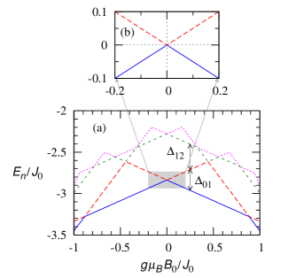
Figure 13: (Color online) (a) A few lowest energy levels of an odd-size chain with $N=7$ as a function of $B_{0}$. The two lowest levels around $B_{0}$ form up and down states of an effective single spin. Two gaps, $\Delta_{01}$ and $\Delta_{12}$ are indicated. (b) A magnified plot of the two lowest levels, offset against the ground state energy $E_{0}/J_{0}=-2.83624$ at $B_{0}=0$, shows a Zeeman splitting of a single spin $1/2$.

Two important energy scales for an odd-size chain are the energy gaps $\Delta_{01}$ and $\Delta_{12}$. The energy gap $\Delta_{12}$ gives the splitting between the ground and excited manifolds. The fact that $\Delta_{01}$ is given by the Zeeman splitting at low fields signifies that the doublet can be considered an effective spin-1/2. Figure 14 shows how the description of the odd-size chain as an effective single spin is limited by its size $N$. While the Zeeman splitting $\Delta_{01}$ is independent of the size $N$ of the spin chain around zero magnetic field, the range of the magnetic field $B_{0}$, within which the effective spin picture is valid, does depend on $N$. The crossover behavior in $\Delta_{01}$ occurs at smaller $B_{0}$ for larger $N$ because the manifold splitting, $\Delta_{12}\sim 1/N$, decreases with $N$.

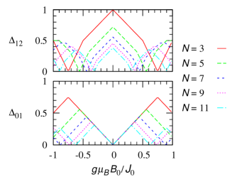
Figure 14: (Color online) Two energy gaps, $\Delta_{01}$ and $\Delta_{12}$ measured in units of $J_{0}$ are plotted as a function of $B_{0}$ for $N=3,5,7,9,11$.

Now that we have established the fact that an odd-size spin chain can be considered as an effective spin-1/2 at low energy, we can construct an effective qubit-bus Hamiltonian within the Hilbert space spanned by the bus ground doublet states and the qubit states. With the doubly degenerate ground states $|{0;\pm\tfrac{1}{2}}\rangle$ of the odd-size bus, the projection operator $P$ is written as

$$P=\mathbb{I}_{A,B}\otimes\left(\,|{0;\tfrac{1}{2}}\rangle\langle{0;\tfrac{1}{2}}|+|{0;-\tfrac{1}{2}}\rangle\langle{0;-\tfrac{1}{2}}|\,\right)_{C}$$ (23)

The effective Hamiltonian to the first order in $H_{QC}$ is

$$H_{\rm eff}^{(1)}=PHP=PH_{0}P+PH_{1}P\,,$$ (24)

where $PH_{0}P$ gives rise to a constant energy shift. In an external magnetic field, it also gives the Zeeman interaction of the effective spin-1/2 system of the spin bus or qubits, $g\mu_{B}\,{\bf B}\cdot{\bf S}_{C}$ or $g\mu_{B}\,{\bf B}\cdot{\bf S}_{\alpha}$ with the external field. With $B_{0}=0$, the first-order effective Hamiltonian Friesen07 is only given by $PH_{1}P$, and takes the form

$$H_{\rm eff}^{(1)}=J^{(1)}_{A,i}\,{\bf S}_{A}\cdot{\bf S}_{C}+J^{(1)}_{B,j}\,{\bf S}_{B}\cdot{\bf S}_{C}\,,$$ (25)

where the effective coupling between qubit $\alpha$ and the spin-bus $C$ is given by

$$J_{\alpha,i}^{(1)} =J_{\alpha,i}\,m_{i}\,,$$ (26a)

$$m_{i} =\langle{0;\tfrac{1}{2}}|\sigma_{iz}|{0;\tfrac{1}{2}}\rangle=-\langle{0;-\tfrac{1}{2}}|\sigma_{iz}|{0;-\tfrac{1}{2}}\rangle$$

$$=\langle{0;\tfrac{1}{2}}|\sigma_{ix}|{0;-\tfrac{1}{2}}\rangle\,,$$ (26b)

where $J_{\alpha,i}$ is the bare coupling between the $i$th spin of the chain and the external qubit $\alpha$, and $m_{i}$ is the dimensionless local magnetic moment at the site $i$ of the chain in the ground state. In the case of $N=3$, Equation (22) gives the local magnetic moments, $m_{1}=2/3,\,m_{2}=-1/3,\,m_{3}=2/3$, with $m_{1}+m_{2}+m_{3}=1$. The effective Hamiltonian  (25) shows again that an odd-size chain acts as an effective spin-1/2 particle that couples to the external qubits $A$ and $B$, as illustrated in Fig. 1.

The effective Hamiltonian to second-order in $H_{1}$, which is needed for longer-time operations, is given by Oh11

$$H_{\rm eff}^{(2)}=J^{(1)}_{A,i}\,{\bf S}_{A}\cdot{\bf S}_{C}+J^{(1)}_{B,j}\,{\bf S}_{B}\cdot{\bf S}_{C}+J^{(2)}_{i,j}\,{\bf S}_{A}\cdot{\bf S}_{B},$$ (27)

where the RKKY-like second-order coupling $J^{(2)}_{i,j}$ is Oh10 ; Oh11 ; RKKY

$$J^{(2)}_{i,j}\equiv\frac{J_{A,i}J_{B,j}}{2}\sideset{}{{}^{\prime}}{\sum}_{n}\frac{\langle{0}|\sigma_{i\mu}|{n}\rangle\langle{n}|\sigma_{j\mu}|{0}\rangle}{E_{0}-E_{n}}\,.$$ (28)

Here $E_{n}$ are the energy levels and $|{n}\rangle$ are the eigenstates of $H_{C}$ omitting the magnetic quantum number. The summation with a prime indicates the exclusion of the ground states. While the exact calculation of $J^{(2)}_{i,j}$ requires complete information of the eigenvalues and eigenstates of the chain, an approximate form can be obtained with only the ground state and the excitation gap. Using the closure relation $\sum|n\rangle\langle n|=1$, where $n$ sums through all the isolated-chain eigenstates, we obtain

$${J^{(2)}_{i,j}}/{(J_{A,i}J_{B,j})}$$

$$\approx\frac{1}{2\Delta_{12}}\Bigl{(}\langle{0}|\sigma_{iz}|{0}\rangle\langle{0}|\sigma_{jz}|{0}\rangle-\langle{0}|\sigma_{iz}\,\sigma_{jz}|{0}\rangle\Bigr{)}\,,$$ (29)

where $|{0}\rangle$ refers to $|{0;\pm\frac{1}{2}}\rangle_{C}$. In other words, the second-order coupling $J^{(2)}_{i,j}$ can be approximated by the difference between the spin-spin correlation function and a product of local magnetic moments of the ground state of the odd-size chain. The competition between these two terms leads to decaying oscillations in $J_{i,j}^{(2)}$. Note that a phase slip occurs when the qubit separation reaches a certain range, as discussed in Ref. Oh11, .

A.2 The Effective Hamiltonian with an Even-Size Bus

In an even-size chain with antiferromagnetic couplings, the spins are completely compensated, so that the chain has a non-degenerate ground state with both zero total magnetic moment, $|{n=0;S_{z}=0}\rangle_{C}$, and zero local magnetic moment, $\langle{0;0}|\sigma_{\mu,i}|{0;0}\rangle=0$. These properties of the even-size chain can be illustrated with the simplest case of $N=2$, when the ground state is the singlet state $|{n=0;S_{Z}=0}\rangle=\frac{1}{\sqrt{2}}(|{0,1}\rangle-|{1,0}\rangle)$. In Fig. 15 we plot the lowest energy levels of an even-size chain with $N=8$ as a function of the external magnetic field $B_{0}$. For small $B_{0}$, the non-degenerate ground state with $S_{z}=0$ is separated from the excited states by the gap $\Delta_{01}$. Similar to the odd-size chain, this gap and the field range before level crossing is limited by the size of the chain, as shown in Fig. 16.

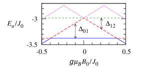
Figure 15: (Color online) The four lowest energy levels of an even-size chain with $N=8$ as a function of $B_{0}$. The two lowest energy gaps, $\Delta_{01}$ and $\Delta_{12}$ in units of $J_{0}$ are indicated.

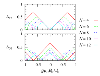
Figure 16: (Color online) The two lowest energy gaps, $\Delta_{01}$ and $\Delta_{12}$, of even-size chains with $N=4,6,8,10,12$, as functions of $B_{0}$.

Protected by the $\Delta_{01}$ gap, the low-energy Hilbert space we are interested in is spanned by the ground state of the even-size chain and the qubit basis states. The projection operator takes the form $P=\mathbb{I}_{AB}\otimes\left(|{0;0}\rangle\langle{0;0}|\right)_{C}$. The first order term in Eq. (21) is $PHP=PH_{0}P+PH_{1}P=E_{0}P$, which is just a constant energy shift. In other words, the first order perturbation term for an even-size chain induces no qubit-bus couplings, since the bus ground state by itself cannot have any dynamics. The second-order perturbation term is obtained in the same way as in the case of an odd-size chain. The effective Hamiltonian to second order in $H_{1}$ is Oh10

$$H_{\rm eff}^{(2)}=J^{(2)}_{i,j}\,{\bf S}_{A}\cdot{\bf S}_{B}\,,$$ (30)

where the RKKY-like coupling $J^{(2)}_{i,j}$ has the same form as Eq. (28), although the prime here would exclude only a single ground state. Similar to the case of the odd-size chain, $J^{(2)}_{i,j}$ can be approximated as

$${J^{(2)}_{i,j}}/{(J_{A,i}J_{B,j})}\approx-\frac{1}{2\Delta_{01}}\,\langle{0;0}|\sigma_{iz}\,\sigma_{jz}|{0;0}\rangle\,,$$ (31)

where $\Delta_{01}$ is the energy gap between the ground state and the first excited state, and $\langle{0;0}|\sigma_{iz}\,\sigma_{jz}|{0;0}\rangle$ is the spin-spin correlation function of the ground state of the chain. There is no contribution from local magnetic moments here since they vanish in the ground state of an even-size bus.

Appendix B Absence of effect on ground state splitting of an odd-size bus by random exchange couplings

Here we prove that for an odd-size spin chain, the energy splitting $\Delta_{01}$ of the ground doublet states at low uniform magnetic fields is independent of the randomness in the inter-node exchange coupling $J_{i}$. With $B_{i}=B_{0}$, the Hamiltonian (10) is

$$H_{C} =H_{C}^{(0)}+V\,,$$ (32)

where $H_{C}^{(0)}$ is the unperturbed Hamiltonian (2), and the perturbation $V$ is given by

$$V=\sum_{i=1}^{N-1}\delta J_{i}\,{\mathbf{s}}_{i}\cdot{\mathbf{s}}_{i+1}\,.$$ (33)

The two lowest eigenstates of the unperturbed Hamiltonian $H_{C}^{(0)}$ are $|{0;-\tfrac{1}{2}}\rangle=|{0^{(0)}}\rangle$ and $|{1;\tfrac{1}{2}}\rangle=|{1^{(0)}}\rangle$, when the magnetic field is applied in the positive $z$ direction, and the corresponding eigenenergies are $E_{0}^{(0)}$ and $E_{1}^{(0)}$. For the perturbed Hamiltonian $H_{C}$, we denote the two lowest eigenstates by $|{0}\rangle$ and $|{1}\rangle$, respectively, and the corresponding eigenvalues by $E_{0}$ and $E_{1}$. By definition, the energy gap $\Delta_{01}$ of $H_{C}$ can be expressed as

$$\Delta_{01}\equiv E_{1}-E_{0}=\Delta_{01}^{(0)}+(\delta E_{1}-\delta E_{0})\,,$$ (34)

where $\Delta_{01}^{(0)}=E_{1}^{(0)}-E_{0}^{(0)}$ is the lowest energy gap of the unperturbed Hamiltonian $H_{C}^{(0)}$, which is a Zeeman gap. The energy shifts of the two lowest levels, $\delta E_{0}\equiv E_{0}-E_{0}^{(0)}$ and $\delta E_{1}\equiv E_{1}-E_{1}^{(0)}$, caused by the perturbation $V$, i.e., fluctuations $\delta J_{i}$, are given by Kittel

$$\delta E_{0}=\frac{\langle{0^{(0)}}|V|{0}\rangle}{\langle 0^{(0)}|0\rangle}\,,\quad\delta E_{1}=\frac{\langle{1^{(0)}}|V|{1}\rangle}{\langle 1^{(0)}|1\rangle}\,.$$ (35)

Their difference $\delta E_{1}-\delta E_{0}$ is thus

$$\delta E_{1}-\delta E_{0}=\frac{\langle{1^{(0)}}|V|{1}\rangle}{\langle 1^{(0)}|1\rangle}-\frac{\langle{0^{(0)}}|V|{0}\rangle}{\langle 0^{(0)}|0\rangle}$$ (36a)

$$= \sum_{i=1}^{N-1}\delta J_{i}\left[\frac{\langle{1^{(0)}}|{\bf s}_{i}\cdot{\bf s}_{i+1}|{1}\rangle}{\langle 1^{(0)}|1\rangle}-\frac{\langle{0^{(0)}}|{\bf s}_{i}\cdot{\bf s}_{i+1}|{0}\rangle}{\langle 0^{(0)}|0\rangle}\right]\,.$$ (36b)

Since $[H_{C},S_{z}]=0$, the two lowest states, $|{0}\rangle$ and $|{1}\rangle$, (also $|{0^{(0)}}\rangle$ and $|{1^{(0)}}\rangle$) of an odd-size bus are spin-flipped states of each other, so that the bracket part in the above equation vanishes, which leads to $\delta E_{1}-\delta E_{0}=0$. This means that the two lowest energy states fluctuate together, as shown in Fig. 2 (a), so that their difference, i.e., the Zeeman energy gap, does not change.

We have thus proven that the Zeeman energy splitting $\Delta_{01}$ of the ground doublet states is invariant over random exchange couplings $J_{i}$. Consequently, the odd-size chain with random exchange couplings can still be regarded as an effective single spin $1/2$ in the low energy limit.

Appendix C Scaling Properties of Spin Buses

In this Appendix we discuss the scaling properties of a spin chain as a quantum data bus. While the Heisenberg spin-1/2 chain is exactly solvable with Bethe ansatz, Bethe only partial information about the ground state and the elementary excitations are available. Various numerical approaches have been applied to this system since Bonner and Fisher’s pioneering work.Bonner Although there has been tremendous advances in computational power, the exact diagonalization method can only handle a spin-$1/2$ system with sizes of up to $N\sim 40$, depending on the number of eigenvalues and eigenstates to be calculated. Indeed, one could consider such limitations as one of the motivations for building a quantum computer. Below we present our results for spin chains with $N$ up to 20.

Calculation of the first-order qubit-bus effective coupling of Eq. (26) needs only knowledge on the ground state of an odd-size chain. On the other hand, calculation of the second-order coupling, Eq. (28), requires the full knowledge of the eigenvalues and eigenstates of the spin chain. We have solved the full spectrum of spin chains with sizes of up to $N=14$ on a personal computer using LAPACK lapack , and obtained a few lowest energy eigenvalues and eigenstates for spin chains with sizes up to $N=20$ using PRIMME. Stathopoulos11

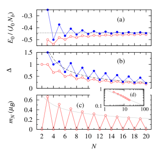
Figure 17: (Color online) (a) The ground state energy $E_{0}/J_{0}$ per bond of the open chains (open red circle) and rings (solid blue circle), (b) the gap $\Delta$ between the ground state and the excited state, (c) the local magnetic moment $m_{N}$ at the end of the open-chain as a function of the size $N$, and (d) a log-log plot of $m_{N}$ for odd-size chains. The dashed line in panel (a) indicates $E_{0}/(J_{0}N)=\frac{1}{4}-\ln 2\approx-0.4431$ obtained from the Bethe ansatz Bethe . The dashed line in panel (b) represents $\Delta/J_{0}=\pi^{2}/N$ from Ref. Lieb61, . The gray lines in panels (c) and (d) represent an $m_{N}\propto 1/\sqrt{N}$ fit.

Figure 17 shows our results on the ground state energy $E_{0}$ per bond, the gap between the ground and the excited states, and the end-point local magnetic moment of the odd-size chain for finite chains of size $N=2$ to $20$. As shown in Fig. 17 (a), the ground state energy per bond approaches the analytic value of $E_{0}/(N_{b}J_{0})=\frac{1}{4}-\ln 2\approx-0.4431$ in the thermodynamics limit, obtained from the Bethe ansatz. Here the number $N_{b}$ of bonds is given by $N_{b}=N-1$ for open chains and $N_{b}=N$ for rings. The ground state energy oscillates, depending on the even-odd parity, as the size of the chain $N$ increases. However, this finite-size effect diminishes in the large-$N$ limit. Figure 17 (b) plots the ground state energy gap $\Delta$ as a function of the size of the chain $N$, with $\Delta=\Delta_{01}$ for even-size chains and $\Delta=\Delta_{12}$ for odd-size chains. The numerical result follows the well-known analytical estimate $\Delta\sim\pi^{2}{J_{0}}/2{N}$ as the size $N$ increases. Lieb61 Although the ground energy $E_{0}$, the spin-spin correlation function for the ground state $\langle{\bf s}_{i}\cdot{\bf s}_{j}\rangle$, and the ground energy gap $\Delta$ are well known, Caspers ; Nolting the scaling property of the local magnetic moment of the odd-size chain is less well understood. Friesen07 Figure 17 (c) plots the dependence of the end-site local magnetic moment on the size $N$. Our numerical data points to a $m_{N}\propto 1/\sqrt{N}$ dependence (possibly slightly faster), as indicated in panel (d) of Fig. 17. Further work is still needed to clarify this $N$-dependence.

References

- (1) D. Loss and D. P. DiVincenzo, Phys. Rev. A 57, 120 (1998).
- (2) J. I. Cirac and P. Zoller, Phys. Rev. Lett. 74, 4091 (1995).
- (3) A. Blais, R.-S. Huang, A. Wallraff, S. M. Girvin, and R. J. Schoelkopf, Phys. Rev. A 69, 062320 (2004).
- (4) S. Bose, Phys. Rev. Lett. 91, 207901 (2003); Contem. Phys. 48, 13 (2007).
- (5) M. Friesen, A. Biswas, X. Hu, and D. Lidar, Phys. Rev. Lett. 98, 230503 (2007).
- (6) S. Oh, M. Friesen, and X. Hu, Phys. Rev. B 82, 140403(R) (2010).
- (7) Y.-P. Shim, S. Oh, X. Hu, and M. Friesen, Phys. Rev. Lett. 106, 180503 (2011).
- (8) S. Oh, L.-A. Wu, Y.-P. Shim, J. Fei, M. Friesen, and X. Hu, Phys. Rev. A84, 022330 (2011).
- (9) S. Oh, Phys. Rev. B 65, 144526 (2002); X. Hu and S. Das Sarma, Phys. Rev. A66, 012312 (2002).
- (10) I.A. Merkulov, A.L. Efros, and M. Rosen, Phys. Rev. B 65, 205309 (2002).
- (11) M. A. Ruderman and C. Kittel, Phys. Rev. 96, 99 (1954); T. Kasuya, Prog. Theor. Phys. 16, 45 (1956); K. Yoshida, Phys. Rev. 106, 893 (1957).
- (12) Quantum Annealing and Related Optimization Methods ed. by A. Das and B. K. Chakrabarti (Springer-Verlag, Berlin, 2005).
- (13) D. Scherrington and S. Kirkpatrick, Phys. Rev. Lett. 35, 1792 (1975).
- (14) S. F. Edwards and P. W. Anderson, J. Phys. F 5, 965 (1975).
- (15) X. Hu and S. Das Sarma, Phys. Rev. Lett. 96, 100501 (2006).
- (16) P. Fulde, Electron Correlations in Molecules and Solids (Springer-Verlag, Berlin, 1991).
- (17) C. Cohen-Tannoudji, J. Dupont-Roc, and G. Grynberg, Atom-Photon Interactions (John Wiley & Sons, New York, 1992)
- (18) H. Bethe, Z. Phys. 71, 205 (1931).
- (19) C. F. Hirjibehedin, C. P. Lutz, and A. J. Heinrich, Science 312, 1021 (2006).
- (20) E. Anderson, Z Bai, C. Bischof, S. Blackford, J. Demmel, J. Dongarra, J. Du Croz, A. Greenbaum, S. Hammarling, A. McKenney, and D. Sorensen, LAPACK Users’ Guide, 3rd Ed. (SIAM, Phiadelphia, 1999).
- (21) C. Kittel, Quantum Theory of Solids (John Wiley & Sons, Inc., New York, 1963).
- (22) Y.-P. Shim et al. (in preparation).
- (23) J. C. Bonner and M. E. Fisher, Phys. Rev. 135, A640 (1964).
- (24) A. Stathopoulos and J. R. McCombs, ACM Transaction on Mathematical Software, 37, 21 (2011).
- (25) E. Lieb, T. Schultz, and D. Mattis, Ann. Phys. (N.Y.) 16, 407 (1961).
- (26) W. J. Caspers, Spin Systems (World Scientific, Singapore, 1989).
- (27) W. Nolting and A. Ramakanth, Quantum Theory of Magnetism (Springer-Verlag, Heidelberg, 2009).