Thesis
figure \chapterstylemadsen \maxsecnumdepthsubsection
This version has been modified for the arXiv. The original version with higher quality figures can be found at http://sns.ias.edu/~rein/ .
![[Uncaptioned image]](/html/1012.0266/assets/x1.png)
Chapter 0 Abstract
The increasing number of discovered extra-solar planets opens a new opportunity for studies of the formation of planetary systems. Their diversity keeps challenging the long-standing theories which were based on data primarily from our own solar system. Resonant planetary systems are of particular interest because their dynamical configuration provides constraints on the otherwise unobservable formation and migration phase.
In this thesis, formation scenarios for the planetary systems HD128311 and HD45364 are presented. N-body simulations of two planets and two dimensional hydrodynamical simulations of proto-planetary discs are used to realistically model the convergent migration phase and the capture into resonance. The results indicate that the proto-planetary disc initially has a larger surface density than previously thought.
Proto-planets are exposed to stochastic forces, generated by density fluctuations in a turbulent disc. A generic model of both a single planet, and two planets in mean motion resonance, being stochastically forced is presented and applied to the system GJ876. It turns out that GJ876 is stable for reasonable strengths of the stochastic forces, but systems with lighter planets can get disrupted. Even if a resonance is not completely disrupted, stochastic forces create characteristic, observable libration patterns.
As a further application, the stochastic migration of small bodies in Saturn’s rings is studied. Analytic predictions of collisional and gravitational interactions of a moonlet with ring particles are compared to realistic three dimensional collisional N-body simulations with up to a million particles. Estimates of both the migration rate and the eccentricity evolution of embedded moonlets are confirmed. The random walk of the moonlet is fast enough to be directly observable by the Cassini spacecraft.
Turbulence in the proto-stellar disc also plays an important role during the early phases of the planet formation process. In the core accretion model, small, metre-sized particles are getting concentrated in pressure maxima and will eventually undergo a rapid gravitational collapse to form a gravitationally bound planetesimal. Due to the large separation of scales, this process is very hard to model numerically. A scaled method is presented, that allows for the correct treatment of self-gravity for a marginally collisional system by taking into account the relevant small scale processes. Interestingly, this system is dynamically very similar to Saturn’s rings.
Chapter 1 Preface and Acknowledgements
This thesis is the result of my own work and includes nothing which is the outcome of work done in collaboration except where specifically indicated.
The formation scenario presented in chapter 3 was done in collaboration with Professor Wilhelm Kley and has been published as a highlighted article in Astronomy and Astrophysics (Rein et al., 2010). The analysis of chapter 4 is based on Rein & Papaloizou (2009). The results of chapter 6 are the outcome of work done in collaboration with Geoffroy Lesur and Zoë Leinhardt. I have contributed more than two thirds to all of these studies. In particular, all simulations and their analysis have been performed by myself. The analytic calculation in appendix 10 has been made by Professor John Papaloizou.
I would like to thank my supervisor, Professor John Papaloizou, for his time and support during the last three years. I would like to thank Zoë Leinhardt, Geoffroy Lesur, Sijme-Jan Paardekooper, Gordon Ogilvie, Aurélien Crida, James Stone and Adrian Barker for stimulating discussions. For proofreading a draft of this thesis, I would like to thank Min-Kai Lin, Adrian Barker, Katy Richardson, Zoë Leinhardt, Aurélien Crida and Chris Donnelly. I appreciate the help of Professor Wilhelm Kley who provided me with data for various code comparisons.
This work was supported by an Isaac Newton studentship and an STFC studentship (ST/F003803/1). I am grateful for financial support for travel from St John’s College Cambridge, the Department of Applied Mathematics and Theoretical Physics, the Institute for Advanced Study in Princeton, AstroSim, the Cambridge Philosophical Society and the Tokyo Institute of Technology. I would also like to thank the Isaac Newton Institute in Cambridge for their support and hospitality during the DDP workshop and associated conferences.
I would like to thank the 800th Anniversary Team for the permission to reprint the drawing of Isaac Newton, copyright Quentin Blake 2009.
Für meine Mutter.
Chapter 2 Introduction
And if the fixed Stars are the Centers of other like systems, these, being form’d by the like wise counsel, must be all subject to the dominion of One, […].
Isaac Newton, General Scholium, translated by Motte, 1729
In 1713 Isaac Newton wrote this sentence in an essay attached to the third edition of his famous Principia Mathematica. In other words, he expected to see planets around other stars. Almost three centuries later, astronomers discovered the first planet beyond our own solar system, a so-called exo-planet. The number of known planets has increased rapidly ever since. To date, 461 extra-solar planets have been discovered (Schneider, 2010). At least 10% of all nearby solar type stars host planets (Cumming et al., 2008). With this tremendous observational success, it is now the theoreticians’ turn to explain the discovered systems. One important aspect is to find out if, and if so why, these systems formed differently compared to the solar system.
In this chapter, first the discoveries of exo-planets in recent years are presented. Then, suggested formation scenarios of planets, planetary systems and their evolution are reviewed.
This thesis discusses stochastic phenomena in a range of astrophysical systems. The analytic model presented in chapter 4 is the key in understanding the effects of stochastic forces and turbulence in those systems. It forms the basis of the physical understanding in many celestial systems in which stochastic forces are present.
A detailed formation scenario of the planetary system HD45364 is presented in chapter 3. In chapter 4 another formation scenario is presented, this time for the planetary system HD128311. Both systems are resonant systems and their dynamical states provide important constraints on their formation history.
HD45364 formed most likely in a massive disc and had a phase of rapid convergent migration. On the other hand, the current observed orbital parameters of the system HD128311 are consistent with the formation in a strongly turbulent disc.
In chapter 5, these formalism developed in chapter 4 is applied to Saturn’s rings and a moonlet. Saturn’s rings also exert stochastic forces. The rings, together with embedded moons, resemble a small scale version of the proto-planetary disc.
Finally, the issue of numerical convergence in simulations of planetesimal formation is discussed in section 6. Planetesimals are likely to form in turbulent proto-stellar discs via gravitational instability. It turns out that the system can be simulated consistently only if the relevant small scale processes are included. The dynamical evolution is then very similar to Saturn’s rings, except that the final clump is gravitationally bound.
In chapter 7 we summarise the results. The main numerical codes that have been used in chapters 3, 4, 5 and 6 are described in the appendices 12 and 11.
1 Methods of detecting extra-solar planets
For thousands of years, the observation of planets was limited to the major planets of our own solar system. Since then, our knowledge of the solar system has been growing constantly and has reached an overwhelming magnitude. However, the fundamental question of whether we inhabit a special place in the universe or not hasn’t been answered yet. This is deeply linked to our spiritual desire to know if there are lifeforms on other planets. Luckily, we are living in a time of great technological and scientific progress and it is not unreasonable to assume that those questions can be answered within the next 50 years.
The first steps have already been taken, namely the discovery of planets beyond our own solar system. Various groups around the world have successfully detected exo-planets using different techniques. Each method has both advantages and disadvantages which will be summarised in this section. This is important because the sparse information that we get from these observations determines the predictability of theoretical studies.
- Radial velocity measurements.
-
Most planets have been discovered by the radial velocity (RV) method. A periodic Doppler shift in the spectral lines of the host star can be measured with high precision spectroscopy. The Doppler effect occurs because the star is moving around the centre of mass (of both the star and the planet). Only the radial part of this movement is measurable. The period of the oscillation is simply the planet’s orbital period. The mass of the star can be calculated by stellar evolution models. If we assume that we observe the system in the plane of the planet’s orbit, we can then use Newton’s third law , where , , and are the masses and velocities of the host star and the planet respectively, to calculate the planet’s mass.
This method biases the detection of massive planets on short orbits (hot Jupiters) as the gravitational influence of the planet on the star (and therefore the measured ) is bigger in those cases. Note that there is a degeneracy in the inclination because it is not possible to measure the non-radial part of the velocity. Thus, we can only get a lower limit on the mass of the planet and the mass might actually be larger:
(1) Because of this degeneracy, only a limited number of parameters can be obtained by the RV method. Finding orbital parameters of multiplanetary systems beyond the planet masses and the orbital periods is even more challenging. Each new planet adds 7 degrees of freedom, such that solutions are highly degenerate. Especially the fitting of the eccentricities is very unreliable (see discussion in chapter 3). Furthermore, it is difficult to find precise orbital parameters for very long period planets as it can take many years to sample a full period of the light curve.
The first extra-solar planet discovered by the radial velocity method is 51 Pegasi b (Mayor & Queloz, 1995).
- Transit light curves.
-
Another method that has been very successful is the transit method. This is mainly due to space based missions such as CoRoT and Kepler. The idea is to find planets by observing variations in the star light caused by transits of planets in front of the host stars. This effect also occurs in our own solar system, known as Mercury and Venus transits. However, transits of extra-solar planets are rare because the host star, the exo-planet and the Earth must be aligned exactly in one line for a transit to occur. The first exo-planet discovered by the transit method is OGLE-TR-56 b (Konacki et al., 2003).
The transit method is capable of measuring the density of exo-planets, a parameter inaccessible to the RV method. It is even possible to do spectroscopy on the atmosphere of the planet during the transit and the secondary transit (when the planet is occulted by the star) to create a temperature map of the exo-planet (Knutson et al., 2007).
Furthermore, the Rossiter-McLaughlin effect allows one to measure the sky projected angle between the orbit and the rotation axis of the host star. To do that, one has to combine transit and RV measurements. A recently submitted paper suggests that a large number of planets might be on retrograde orbits (Triaud et al, in preparation).
Dedicated ground and space based missions promise to detect a large number of planets in the near future. Furthermore, by observing tiny variations in the transit timing (TTV) and transit duration (TDV), it might be possible to find other planets in systems in which only one planet is transiting. Even the possibility to discover exo-moons has been discussed (Kipping et al., 2009).
- Gravitational microlensing.
-
Planets can also be discovered by gravitational microlensing. If the star is aligned in one line with the Earth and a bright object in the background (e.g. another star), the light from the background object bends around the star and can be detected by an increase in luminosity. A planet in an orbit around the star disturbs the light curve and theoretical models can determine the planet’s mass and some orbital parameters. This event happens only once per star, so good timing and a global collaboration is needed to perform a continuous measurement of the light curve. The orbital parameters cannot be determined with high precision because one only obtains a snapshot of the system without any dynamical evolution. The first exo-planet was discovered by gravitational microlensing in 2004 by Bond et al..
- Direct imaging.
-
In 2004 Chauvin et al. reported the first detection of a giant planet candidate by direct imaging. Since then, several planetary systems have been imaged. These are all massive planets, far away from the host star (hundreds of AU). Maybe the most interesting of those planets is Fomalhaut b, which seems to be embedded in a debris disc (Kalas et al., 2008). As all those planets have long orbital periods, it is, similar to the gravitational microlensing method, difficult to determine the precise orbital configuration, especially in multi-planetary systems.
- Pulsar timing.
-
Despite the recent success of the detection methods presented above, the first exo-planet was discovered using the pulsar timing method (Wolszczan & Frail, 1992) by measuring slight variations in the regular timings from a pulsar. This is sensitive down to very small mass planets. However, pulsars are rare compared to normal stars and the focus has shifted away from the pulsar timing method.
2 Observed objects
Extrasolar planets have been observed around a variety of parent stars from pulsars to solar-type stars to M-dwarfs (see e.g. Chauvin et al., 2004; Wolszczan & Frail, 1992) indicating that planet formation is common and successful in a broad range of environments. Almost all extra-solar planetary systems are distinct from the solar system. Many of the detected objects are so-called hot Jupiters. Their size and mass is comparable to Jupiter, but their orbits are very close to their host star ( AU). Most methods described above bias the detection in favour of these objects.
The existence of hot Jupiters was very surprising because in the solar system all gas giants are located beyond several AU. This still results in difficulties for planet formation theories, although planetary migration is one solution, as described below.
Other observed objects are very heavy and are more likely to be brown dwarfs rather than planets. The International Astronomical Union (IAU) defines an extra-solar planet as follows:
Objects with true masses below the limiting mass for thermonuclear fusion of deuterium (currently calculated to be 13 Jupiter masses for objects of solar metallicity) that orbit stars or stellar remnants are planets (no matter how they formed). The minimum mass/size required for an extra-solar object to be considered a planet should be the same as that used in our Solar System. (WGESP, 2003)
Thus, many of the massive objects, at separations of hundreds of AU, detected by direct imaging, could actually be brown dwarfs.
In cases where the planet’s mean density can be observed, evolutionary models seem to be in broad agreement with observations, although many hot Jupiters have a large surface temperature and are subject to tidal heating. Their atmospheres are not well understood and first studies show a broad range of possible configurations. Observations furthermore suggest that their densities might be rather low (see e.g. Anderson et al., 2010).
The Holy Grail for exo-planet hunters is another Earth-like planet that orbits the host star within the habitable zone. At the present day, the planet that is closest to one Earth mass is Gliese 581 e which has a mass of approximately 2 Earth masses (Mayor et al., 2009).
3 Formation of planets
1 Accretion disc
Stars form out of giant gas clouds that become gravitationally unstable. Because of angular momentum conservation, an accretion disc forms around every new star. As the name suggests, an accretion disc will eventually accrete most of its material onto the star, leaving only a small fraction of it as planets or a debris disc in orbit around the star. Observations of accretion rates in proto-planetary discs suggest that accretion timescales are of the order of a few years (Enoch et al., 2008).
Usually one assumes that the Navier-Stokes equations are a good approximation to describe the fluid motion within the disc. However, to reproduce the measured accretion rates, a purely molecular viscosity is not efficient enough. It is generally believed that this large viscosity originates from turbulence (Pringle, 1981). The mass flux in a steady state Keplerian disc is then given by
| (2) |
where is the effective kinematic viscosity and the surface density. From observations of proto-stars, a value of has been inferred, but with considerable uncertainty.
The magneto rotational instability (MRI, Balbus & Hawley, 1991) is the most likely candidate to be responsible for the anomalous value of which is often characterised using the Shakura & Syunyaev (1973) parameter, defined as , with being the local sound speed and being the orbital period. For the most likely situation of small or zero net magnetic flux, recent MHD simulations have indicated . This value is very uncertain when realistic values of the actual transport coefficients are employed due in no small part to numerical resolution issues (see Fromang & Papaloizou, 2007; Fromang et al., 2007). Which parts of proto-planetary discs are adequately ionised, or constitute a dead zone, is also an issue (Gammie, 1996; Sano et al., 2000).
Putting aside all those issues for a moment, the MRI always creates density fluctuations in the disc, resulting in a stochastic force that is exerted on embedded planets which are otherwise decoupled from the gas motion (ignoring migration, which is a laminar effect and acts on timescales much longer than one orbit). In this thesis, we do not attempt to simulate the MRI directly and rather describe it in an empirical way. We therefore avoid all problems mentioned above and can understand the physical scaling of our results. Only two quantities are needed for our analytic model, the root mean square value of the stochastic gravitational force and the corresponding auto correlation time. Laughlin et al. (2004) propose a more complicated model, in which random modes with random decay times create a gravitational potential that is supposed to mimic the MRI. Our, much simpler and more intuitive description, allows us to survey a large parameter space and understand the resulting physical processes, as discussed in chapter 4.
2 Minimum mass solar nebula and snowline
A standard model of a proto-planetary disc assumes a steady state and a vertical equilibrium (see also appendix 2). The gas and dust components are furthermore assumed to be fully mixed. The resulting disc is flared, although still geometrically thin. For sufficiently low mass accretion rates () the dominant heating source is stellar irradiation (Chiang & Goldreich, 1997).
Hayashi (1981) prescribes the so-called minimum mass solar nebula (MMSN) which is comprised of just enough mass to make all planets of the solar system. This model became the standard disc model and has been used excessively in recent years with different normalisations. One can describe the surface density and temperature profiles as
| (3) |
Typical normalisation values at are and . Standard values of range from to , those of from to (Hayashi, 1981; Cuzzi et al., 1993). The typical mass of the disc is about one percent of the stellar mass. Although the choice of disc model is essential for most aspects of planet formation, little emphasis has been placed on alternatives (see e.g. Desch, 2007; Crida, 2009).
To form planets and planetary cores, dust is an important ingredient (see also below). In the model of Hayashi (), the radius at which temperatures drop below 170 K is around 2.7 AU. At larger radii, the temperatures are low enough for water ice to exist. This transition radius is called the snow line. Recent studies, including more detailed models of accretional heating and radiative transfer show that the snow line could come as close as 1 AU (Sasselov & Lecar, 2000).
3 Planet formation mechanism
Planets are believed to form in proto-stellar discs as a natural by-product of star formation. These discs are made of the same material as the star itself: gas and dust. Current theories give two possible explanations of the formation of giant planets inside the disc. Both models favour planet formation at large radii, beyond the snowline. However, it is important to keep in mind that the process of planet formation itself is not directly observable (yet), leaving theory and numerical simulations to fill in the blanks between observations of hot circumstellar discs around young stars and planets orbiting main sequence stars.
Core accretion
One of the most important unanswered questions in the theory of planet formation is to find out what the mechanism for planetesimal formation is, i.e., the process by which the building blocks of planets are formed. In the core accretion model, solid components of the disc stick together, forming bigger and bigger objects until a core of about 15 Earth masses is formed (Bodenheimer & Pollack, 1986; Pollack et al., 1996a). The proto-planet can then start to accrete gas and form a gas giant.
Again, there are two main theories for planetesimal formation via the core accretion model: mutual collisions (e.g., Hayashi et al., 1977) and gravitational instability in the dust layer (Goldreich & Ward, 1973). In the first hypothesis, dust particles grow as the result of accretion-dominated collisions. Although the formation of planetesimals by mutual collisions is consistent with meteoritic evidence, the collision speed between dust particles (or aggregates) must be much slower than the typical velocity dispersion in a standard proto-stellar disc to avoid destructive collisions (Blum & Wurm, 2008). In addition, the planetesimal formation process is so slow that metre-sized particles are in danger of spiralling into the star before growing large enough to decouple from the gas (Weidenschilling, 1977b). Even if km-sized planetesimals were able to form, they would be in danger of being ground down again by mutual collisions (Stewart & Leinhardt, 2009).
Gravitational instability is often considered to be a solution to most of these problems because the intermediate sizes are avoided all together. In this theory, the dust layer becomes dense enough for the Keplerian shear and velocity dispersion of the dust particles to be unable to support the dust against its own self gravity. The dust then collapses into clumps that eventually cool via drag forces and mutual collisions into planetesimals. Many different groups have been working on this subject. Until recently, the focus has been on quiet, non-turbulent, and low density regions of the accretion disc (see e.g., Michikoshi et al., 2009, 2007; Tanga et al., 2004).
However, the turbulent gas in the proto-planetary nebula stirs the dust, which increases the velocity dispersion of the dust particles. Several ideas have been proposed to overcome the turbulence-induced mixing of the dust particles and create localised clumps. For example, Cuzzi et al. (2008) suggest that the same turbulence that stirs the dust on larger scales may also collect the dust particles on small scales. A similar idea was proposed by Johansen et al. (2007), in which dust particles are localised into clumps promoted by both turbulence and the streaming instability (Youdin & Goodman, 2005). These dense clumps then become gravitationally unstable. A third hypothesis suggests that large structures, such as vortices, may be able to collect and protect dust particles from the turbulent background (Barge & Sommeria, 1995; Lyra et al., 2009).
In chapter 6, we focus on the gravitational collapse in a very dense and turbulent region of the proto-planetary disc. We look carefully at the numerical requirements of modelling gravitational instability accurately and test the validity of using super-particles in a high density region. The results suggest that some of the early results of graviational collapse from other authors may have been too optimistic.
Gravitational fragmentation
In this model, gas planets form directly as a result of gravitational instability within the disc (Boss, 2001); no solid core is needed. However, the planet can accrete dust particles later on, and hence form a core.
For the gravitational instability to occur, it is necessary to have a Toomre parameter of order unity (Toomre, 1964). The precise criterion depends strongly on the thermodynamics on the disc, especially the cooling time. However, it is unlikely that the physical conditions in a proto-planetary disc are compatible with this constraint. If so, this is most likely to occur at large radii ( AU). It therefore cannot be the formation mechanism for most discovered exo-planets.
4 Evolution of planetary systems
1 Migration
Many observed planets are very close to their host star. It is implausible that they have formed at such small radii (see section 2), even taking into account the strong selection effect of discovering close in exo-planets (see section 1).
Tidal interactions with the proto-planetary disc give the planet some radial mobility and might therefore be the solution to this problem (Goldreich & Tremaine, 1980). The mutual angular momentum exchange depends on many parameters of both the planet and the disc. Several population synthesis simulations were able to reproduce the observed mass-period distribution using migration (e.g. Ida & Lin, 2004). Planet migration can be classified in the following four main categories.
Type I
Planets are completely embedded in a proto-planetary disc for sufficiently low mass. Density waves are excited in the disc, both interior and exterior to the planet, at so-called Lindblad resonances. The waves carry angular momentum and produce a torque on the planet that leads to planetary migration (Goldreich & Tremaine, 1979). The direction of migration depends on parameters of the disc model such as the gradients of the surface density, sound speed and scale height (Ward, 1997). In most cases, the outer torque is bigger than the inner one and the planet migrates inward. This effect is called type I migration.
If the migration rate is very fast, low mass planets are in danger of spiralling into the star within the disc lifetime. The precise speed and direction in a realistic disc model are still subject to debate, where recently the focus has been on non-isothermal equations of state and the effects of co-rotation torques (Paardekooper et al., 2010; Paardekooper & Papaloizou, 2009).
Type II
If the planet is massive enough, it can open a gap in the disc. For most disc models about a Jupiter mass is needed to clear a clean gap. The process is similar to the gaps opening in Saturn’s rings with moons orbiting within the gap. The gap establishes a flow barrier to the disc material, effectively locking the planet to the viscous disc evolution (Lin & Papaloizou, 1986). Thus, the planet still migrates, the regime being called type II migration. However, the migration timescale is set by the disc evolution timescale which is in general much longer than the type I migration timescale.
Type III
In a disc with a relatively large surface density (several times the MMSN), the density distribution in the co-orbital region of the planet can be asymmetric. This leads to a self-sustained torque that is proportional to the migration rate. In this regime, called type III migration, the planet can fall inward on a timescale much shorter than the disc evolution time obtained for type II migration, even shorter than the timescales associated with type I migration. The planet moves faster than the disc can respond to its perturbation, thus maintaining an asymmetry. The net torque can cause both inward or outward migration (Pepliński et al., 2008a, b, c).
In chapter 3 we present the first observable indication that type III migration is indeed responsible for shaping planetary systems.
Type IV
The different migration regimes have all been studied in quiet non-turbulent discs. However, a proto-planetary disc is thought to be at least partially turbulent (see section 1). Assuming the simplest scenario in which the effects of turbulence and the net migration are separable, one can describe the stochastic migration as a diffusion process in a distribution of planets on top of the net orbital migration, described above. We call this regime type IV.
This idea leads to a Fokker-Planck description (Adams & Bloch, 2009). There are two limits to this approach. The first, in which the net migration dominates and the effects of turbulence are negligible (mostly for heavy planets). The second, in which the net migration can be ignored and the turbulence driven diffusion dominates on short timescales (mostly for small mass planets and planetesimals). We are in an intermediate regime if the migration and diffusion timescales are comparable. It is unlikely that the interplay of stochastic migration and net migration plays an important role in determining the final semi major axis of planets because the associated timescales would have to be very similar. However, resonant systems are more sensitive to stochastic forces and might therefore provide observational constraints on the strength of turbulence that was present at early times.
So far, only preliminary work has been done on studying the effect of the turbulence on resonances (Adams et al., 2008; Nelson & Papaloizou, 2004). If the turbulence is active long enough, it will eventually kick the planets out of resonance. This might happen even if the stochastic forces are not strong enough to cause significant orbital migration. However, the timescale needed for destroying a resonance is not well constrained. New results on this issue are presented in chapter 4.
5 Mean motion resonances
Resonances in celestial mechanics can occur when there is a simple numerical relation between two frequencies (Murray & Dermott, 2000). For example, a planet could feel a periodic gravitational force from another planet that is a multiple of its own orbital frequency. This can either lead to an unstable situation in which angular momentum is exchanged until the resonance ceases to exist or a planet gets ejected from the system, or a stable configuration.
Resonances can form when dissipative forces act on the planets, for example in a proto-planetary disc (see e.g. Malhotra (1993) and appendix 9). When there are two (or more) planets in the disc, the migration rates might differ for various reasons. One possibility is that the planets are in different migration regimes (see section 1). The resulting differential migration changes the ratio of orbital periods and the ratio of semi major axes . These ratios are related by Kepler’s third law, .
The planets can become locked into a mean motion resonance (MMR) if the ratio of orbital periods gets close to a rational number with small integers and , e.g. or . The numbers and can be interpreted as the number of completed orbits after the same time. Some of these resonances are stable and planets can stay in resonance over a long period of time, migrating together and keeping the ratio of their orbital periods constant. Beside the presence of Hot Jupiters, resonance capturing is admitted as strong evidence that planets undergo a phase of orbital migration. This idea was successful in explaining the observed resonant multi-planet systems GJ876 and 55 Cancri (Lee & Peale, 2001; Snellgrove et al., 2001) which are in a 2:1 resonance. In chapter 3, we discuss the first successful formation scenario for a system that is in a 3:2 resonance.
Chapter 3 The dynamical origin of the multi-planetary system HD45364
Truth is ever to be found in simplicity, and not in the multiplicity and confusion of things.
Issac Newton, unpublished manuscript, Frank E. Manuel 1974
The recently discovered planetary system HD45364, which consists of Jupiter- and Saturn-mass planets, is very likely in a 3:2 mean motion resonance. The standard scenario for forming planetary commensurabilities involves convergent migration of two planets embedded in a proto-planetary disc. However, when the planets are initially separated by a period ratio larger than two, convergent migration will most likely lead to a stable 2:1 resonance, incompatible with current observations.
Rapid type III migration of the outer planet crossing the 2:1 resonance is one possible way around this problem. Here, we investigate this idea in detail. We present an estimate of the required convergent migration rate in section 2 and confirm this with N-body simulations in section 2 and hydrodynamical simulations in section 3. If the dynamical history of the planetary system had a phase of rapid inward migration that forms a resonant configuration as we suggest here, then we predict that the orbital parameters of the two planets will always be very similar and should show evidence of that.
We use the orbital parameters from our simulation to calculate a radial velocity curve and compare it to observations in section 5. Our model provides a fit that is as good as the previously reported one. However, the eccentricities of both planets are considerably smaller and the libration pattern is different. Within a few years, it will be possible to observe the planet-planet interaction directly and thus distinguish between these different dynamical states.
This is the first prediction of orbital parameters for a specific extra-solar planetary system derived from planet migration theory alone. It provides strong evidence on how the system formed.
1 The planetary system HD45364
1 The standard formation scenario and its problems
The planets in this system have masses of and and are orbiting the star at a distance of and , respectively (Correia et al., 2008). The period ratio is close to . This alone does not imply that the planets are in a 3:2 mean motion resonance. However, a stability analysis shows that the three body system (two planets and a star) is only stable if the planets are in a 3:2 mean motion resonance. Furthermore, the region of greatest stability also contains the best statistical, Keplerian fit to the radial velocity measurements (Correia et al., 2008).
In the core accretion model, a solid core is firstly formed by dust aggregation. After a critical core mass is attained (Mizuno, 1980), the proto-planet accretes a gaseous envelope from the nebula (Bodenheimer & Pollack, 1986).
As explained in more detail in section 2, the planets have most likely formed further out in cooler regions of the proto-stellar disc as water ice, which is an important ingredient for dust aggregation, can only exist beyond the snow line. The snow line is generally assumed to be at radii larger than (Sasselov & Lecar, 2000).
When the planets have obtained a substantial part of their mass, they migrate due to planet disc interactions (see section 1). Although the details of this process are still being hotly debated, the existence of many resonant multiplanetary systems and hot Jupiters supports this idea and suggests that planets preferably migrate inwards. Both planets in the HD45364 system are inside the snow line, implying that they should have migrated inwards significantly.
The migration rate depends on many parameters of the disc such as surface density, viscosity, and the mass of the planets. The planets are therefore in general expected to have different migration rates, which leads to the possibility of convergent migration. In this process the planets approach orbital commensurabilities. If they do this slowly enough, resonance capture may occur (Goldreich, 1965), after which they migrate together maintaining a constant period ratio thereafter.
Studies by several authors have shown that when two planets, either of equal mass or with the outer one more massive, undergo differential convergent migration, capture into a mean motion commensurability is expected provided that the convergent migration rate is not too fast (Snellgrove et al., 2001). The observed inner and outer planet masses are such that, if (as is commonly assumed for multiplanetary systems of this kind) the planets are initially separated widely enough that their period ratio exceeds a 2:1 commensurability is expected to form at low migration rates (e.g. Nelson & Papaloizou, 2002; Kley et al., 2004).
Pierens & Nelson (2008) have studied a similar scenario where the goal was to resemble the 3:2 resonance between Jupiter and Saturn in the early solar system. They also find that the 2:1 resonance forms in early stages; however, in their case the inner planet had the higher mass, whereas the planetary system that we are considering has the heavier planet outside. In their situation the 2:1 resonance is unstable, enabling the formation of a 3:2 resonance later on, and the migration rate can stall or even reverse (Masset & Snellgrove, 2001).
For the planetary system HD45364, this standard picture poses a new problem. Assuming that the planets have formed far apart and were not much smaller during the migration phase, the outcome is almost always a 2:1 mean motion resonance, not 3:2 as observed. The 2:1 resonance that forms is found to be extremely stable. One possible way around this is a very rapid convergent migration phase that passes quickly through the 2:1 resonance.
2 Avoiding the 2:1 mean motion resonance
We found that, if two planets with masses of the observed system are in a 2:1 mean motion resonance, which has been formed via convergent migration, this resonance is very stable. An important constraint arises, because at the slowest migration rates, the 2:1 resonance is expected to form rather than the observed 3:2 commensurability provided the planets start migrating outside any low-order commensurability.
We can estimate the critical relative migration timescale above which a 2:1 commensurability forms with the condition that the planets spend at least one libration period migrating through the resonance. The resonance’s semi-major axis width associated with the 2:1 resonance can be estimated from the condition that two thirds of the mean motion difference across be equal in magnitude to over the libration period. This gives
| (1) |
where and are the semi major axis and the mean motion of the outer planet, respectively. The libration period can be expressed in terms of the orbital parameters (see e.g. Goldreich, 1965; Rein & Papaloizou, 2009, and also chapter 4) but is here measured numerically, for convenience. If we assume the semi-major axes of the two planets evolve on constant (but different) timescales and , the condition that the resonance width is not crossed within a libration period gives
| (2) |
to pass through the 2:1 MMR.
If the planets of the HD45364 system are placed in a 2:1 resonance with the inner planet located at , the libration period is found to be approximately . Thus, a relative migration timescale shorter than is needed to pass through the 2:1 resonance. For example, if we assume that the inner planet migrates on a timescale of 2000 years, then the outer planet has to migrate with a timescale of
| (3) |
2 N-body simulations
We ran -body simulations to explore the large parameter space and confirm the estimate from the previous section. In an N-body simulation all objects (stars, planets) are treated as point masses interacting only gravitationally with each other. To model the planet-disc interaction, one can explicitly add dissipative and stochastic forces. Thus, the total force acting on an object is a sum of the following terms
| (4) |
The first term is due to the gravitational interaction. In units where we have
| (5) |
where we sum over all particles in the system, except the -th particle. In the heliocentric coordinate system which is used here, the star is located at a fixed position at . That brings about an additional indirect term as we are in an accelerated, non-inertial frame,
| (6) |
The next two terms in eqation 4 are due to the laminar planet-disc interaction. In a first approximation the interaction damps the semi-major axis and the eccentricity on time scales and , respectively. The exact terms depend on the orbital parameters of the planet and are given in appendix 9. It is common practice to define the ratio between the timescales . To obtain those timescales, we have to compare the N-body simulations to full hydrodynamical simulations which will be done in the following section. An N-body simulation is much faster than a hydrodynamical simulation and thus can be integrated over a longer time span. This is essential because resonance capturing and migration act on timescales years and we might even want to integrate over millions of years. The last term in equation 4 adds stochastic forces, simulating the turbulent nature of proto-planetary discs. The implementation is discussed in chapter 4.
Newton’s second law together with equation 4 forms a system of ordinary differential equations. To solve them, a new N-body code has been developed which is highly modular and easily expandable. It incorporates different modules for stochastic forces, migration, data output and time-stepping.
The choice of integrator depends on the problem. The following algorithms have been implemented:
- Runge-Kutta Method (RK4)
-
The classical, fourth order Runge-Kutta method is a widely-used standard integrator. It is an explicit method that needs four function evaluations per time-step. The main disadvantage of the RK4 method is the fixed time-step. We have to set a specific value at the beginning of the computation that is not refined later on.
- Runge-Kutta-Fehlberg Method (RKF45)
-
The Runge-Kutta-Fehlberg method is a fifth order explicit method with an embedded fourth order method (Fehlberg, 1969). We can use the two different results to estimate the numerical error and a new time-step. We repeat the step with a smaller time-step if the error is larger than a specified limit .
- Midpoint Method
-
The midpoint method belongs to the class of second order Runge-Kutta methods. Due to the low order it is not efficient to use it on its own, but it is used as a sub-timestep integrator by the Bulirsch-Stoer Method.
- Bulirsch-Stoer Method (BS)
-
This method (Stoer & Bulirsch, 2002; Press et al., 1992) is based on a stepwise extrapolation. For each time-step we calculate the new positions and velocities several times with different sub-time-steps using the modified midpoint method. We then perform an extrapolation to a perfect sub-step in the limit where . This allows the use of very large time-steps while still obtaining a high accuracy. We can also use the extrapolation to estimate the error and thus make the method adaptive.
The code has been used in Rein & Papaloizou (2009) and Rein et al. (2010), usually with the Bulirsch-Stoer integrator and a precision of . A symplectic integrator has not been implemented, although it would have better long term conservation properties. This is because the integrator would formally not be symplectic any more once velocity dependent forces have been added. This is the case in all simulations presented here, which include either migration or stochastic forces. Note that in some cases it is possible to find a symplectic integrator for systems with velocity dependent forces, for example for Hill’s equations (Quinn et al., 2010). Such an integrator (a modified version of the leap-frog algorithm) has been used in shearing sheet calculations of planetary rings, presented in chapter 5.
1 Parameter space survey
[Period ratio as a function of time (-axis) and migration timescale of the outer planet (-axis).] \subbottom[Eccentricity of the inner planet as a function of time (-axis) and migration timescale of the outer planet (-axis).] \subbottom[Eccentricity of the outer planet as a function of time (-axis) and migration timescale of the outer planet (-axis).]
[Period ratio as a function of time (-axis) and migration timescale of the outer planet (-axis).] \subbottom[Eccentricity of the inner planet as a function of time (-axis) and migration timescale of the outer planet (-axis).] \subbottom[Eccentricity of the outer planet as a function of time (-axis) and migration timescale of the outer planet (-axis).]
[Period ratio as a function of time (-axis) and migration timescale of the outer planet (-axis).] \subbottom[Eccentricity of the inner planet as a function of time (-axis) and migration timescale of the outer planet (-axis).] \subbottom[Eccentricity of the outer planet as a function of time (-axis) and migration timescale of the outer planet (-axis).]
With the new N-body code, we can now easily scan the parameter space and confirm the analytic estimate of the critical migration rate needed to capture into the 3:2 resonance.
We place both planets on circular orbits at and initially. The migration timescale for the inner planet is fixed at , while the migration timescale for the outer planet is varied. In figures 1, 2 and 3 we plot the period ratio and the eccentricities of both planets as a function of time for different migration timescales . In all cases, there is a sharp transition of the final resonant configuration from 2:1 to 3:2 at around . This value agrees closely with the analytic estimate given by equation 3. Note that once the planets are in resonance, the eccentricities quickly reach an equilibrium value as the planets migrate adiabatically.
In figure 2 the eccentricity damping corresponds to and is therefore three times stronger than in figure 1. A value of is rather high and probably unphysical. It can be seen that a smaller eccentricity damping timescale pushes the boundary towards a longer migration time-scale. Although this effect is rather weak (a three times stronger eccentricity damping shifts the boundary by only 4%), it can be easily understood within the toy model presented above. The eccentricities have to rise quickly, while the planets are within the resonance width. This is more difficult for short eccentricity damping timescales.
In figure 3 the eccentricity damping corresponds to and is therefore ten times weaker than in figure 1. Again, a value of is probably unphysical. This results in a rapid rise of eccentricities as soon as the planets are in resonance. Systems that are in a 3:2 resonance become unstable within a few thousand years. On the other hand, systems that are in a 2:1 resonance remain stable, although eccentricities are high ().
The results show clearly that, if the planets begin with a period ratio exceeding two, to get them into the observed 3:2 resonance, the relative migration time has to be shorter than what is obtained from the standard theory of type II migration applied to these planets in a standard model disc (Nelson et al., 2000). In that case one expects this timescale to be larger than years, being effectively the disc evolution timescale. However, it is possible to obtain the required shorter migration timescales in a massive disc in which the planets migrate in a type III regime (see e.g. Masset & Papaloizou, 2003; Pepliński et al., 2008a). In this regime, the surface density distribution in the co-orbital region is asymmetric, leading to a large torque which is able to cause the planet to fall inwards on a much shorter timescale than the disc evolution time obtained for type II migration. Other parameters such as the eccentricity damping timescale do not have a strong effect on capture probabilities.
We explore the feasibility of this scenario in more detail in the following sections.
3 Hydrodynamical simulations
| Run | Result | |||||
|---|---|---|---|---|---|---|
| F1 | 0.05 | 0.6 | 0.001 | 768 | 768 | 3:2 |
| F2 | 0.05 | 0.6 | 0.0005 | 768 | 768 | 3:2 D |
| F3 | 0.05 | 0.6 | 0.00025 | 768 | 768 | 2:1 D |
| F4 | 0.04 | 0.6 | 0.001 | 768 | 768 | 3:2 D |
| F5 | 0.07 | 0.6 | 0.001 | 768 | 768 | 3:2 |
| R1 | rad | 1.0 | 0.0005 | 300 | 300 | 3:2 |
Two-dimensional, grid-based hydrodynamic simulations of an accretion disc with two gravitationally interacting planets were performed to test the rapid migration hypothesis. The simulations performed here are similar in concept to those performed by Snellgrove et al. (2001) of the resonant coupling in the GJ876 system that may have been induced by orbital migration resulting from interaction with the proto-planetary disc. We performed studies using the FARGO code (Masset, 2000) with a modified locally isothermal equation of state. Those runs are indicated by the letter F.
Willy Kley also ran simulations including viscous heating and radiative transport using the RH2D code. Those runs are indicated by the letter R and more details can be found in Rein et al. (2010).
Further simulations have been performed with a new hydrodynamics code called Prometheus, which is described in appendix 12. The code is similar to FARGO, using operator splitting, a staggered grid and fast orbital advection. However, it it can be run in two dimensions (cylindrical grid) and in three dimensions (spherical coordinates). Furthermore, it includes a particle and an MHD module.
1 Initial configuration and computational set up
We use a system of units in which the unit of mass is the central mass the unit of distance is the initial semi-major axis of the inner planet, and the unit of time is . Thus the orbital period of the initial orbit of the inner planet is in these dimensionless units. The parameters for some of the simulations we conducted, as well as their outcomes, are given in table 1.
In all simulations presented here, the mass ratio of the inner and outer planet is and , respectively. The mass ratios adopted are those estimated for HD45364. The initial separation of the planets is . The viscosity is chosen to be . The simulations have the inner and outer boundary of the 2D grid at and , respectively. In all simulations, a smoothing length has been adopted, where is the disc thickness at the planet’s position. This corresponds to about 4 zone widths in a simulation with a resolution of . The role of the softening parameter that is used in two-dimensional calculations is to account for the smoothing that would result from the vertical structure of the disc in three dimensional calculations (e.g. Masset et al 2006). We find that the migration rate of the outer planet is only independent of the smoothing length if the sound speed is given by equation 7 (see next section).
The planets are initialised on circular orbits, slowly turning on their mass in the first 5 orbits. We assume there is no mass accretion, so that these remain fixed in the simulation (see discussion in Pepliński et al., 2008a, and also Sect. 4). The initial surface density profile is constant, and tests indicate that varying the initial surface density profile does not change the outcome very much. The total disc mass in the simulations listed in table 1 ranges from 0.014 to 0.055 solar masses. Non-reflecting boundary conditions have been used throughout this chapter.
2 Equation of state
The outer planet is likely to undergo rapid type III migration, and the co-orbital region will be very asymmetric. We find, in accordance with Pepliński et al. (2008a), that the standard softening description does not lead to convergent results (for a comparative study see Crida et al., 2009). Because of the massive disc, a high density spike develops near the planet. Any small asymmetry will then generate a large torque, leading to erratic results. We follow the prescription of Pepliński et al. (2008a) and increase the sound speed near the outer planet since the locally isothermal model breaks down in the circum-planetary disc. The new sound speed is given by
| (7) |
where and are the distance to the star and the outer planet, respectively. and are the Keplerian angular velocity and and are the aspect ratio, both of the circumstellar and circum-planetary disc, respectively. The parameter is chosen to be , and the aspect ratio of the circum-planetary disc is . The sound speed has not been changed in the vicinity of the inner, less massive planet as it will not undergo type III migration and the density peak near the planet is much lower.
In radiative simulations (R), we go beyond the locally isothermal approximation and include the full thermal energy equation, which takes the generated viscous heat and radiative transport into account. In this radiative formulation, the sound speed is a direct outcome of the simulation, so we do not use equation 7 (Rein et al., 2010).
3 Simulation results


We find several possible simulation outcomes. These are indicated in the final column of table 1, which gives the resonance obtained in each case with a final letter D denoting that the migration became ultimately divergent, resulting in a loss of the commensurability. We find that convergent migration could lead to a 2:1 resonance that was set up in the initial stages of the simulation (F3). Cases F1,F2,F4,F5,R1 provide more rapid and consistent convergent migration than F3 and can attain a 3:2 resonance directly.
Thus avoidance of the attainment of sustained 2:1 commensurability and the effective attainment of 3:2 commensurability required a rapid convergent migration, as predicted by the N-body simulations and the analytic estimate (see section 2). That is apparently helped initially by a rapid inward migration phase of the outer planet which shows evidence of type III migration. The outer planet went through that phase in all simulations with a surface density higher than , and a 3:2 commensurability was obtained. Thus, a surface density comparable to the minimum solar nebula (MMSN, Hayashi, 1981), as used in simulation F3, is not sufficient to allow the planets undergo rapid enough type III migration. As soon as the planets approach the 3:2 commensurability, type III migration stops due to the interaction with the inner planet and the outer planet starts to migrate in a standard type II regime.
This imposes another constraint on the long-term sustainability of the resonance. The inner planet remains embedded in the disc and thus potentially undergoes a fairly rapid inward type I migration. If the type II migration rate of the outer planet is slower than the type I migration rate of the inner planet, then the planets diverge and the resonance is not sustained. A precise estimate of the migration rates is impossible in late stages, as the planets interact strongly with the density structure imposed on the disc by each other.
Accordingly, outflow boundary conditions at the inner boundary that prevent the build up of an inner disc are more favourable to the maintenance of a 3:2 commensurability because the type I migration rate scales linearly with the disc surface density. However, those are not presented here, as the effect is weak and we stop the simulation before a large inner disc can build up near the boundary.
The migration rate for the inner planet depends on the aspect ratio . It is decreased for an increased disc thickness (Tanaka et al., 2002). That explains why models with a large disc thickness (F5,R1) tend to stay in resonance, whereas models with a smaller disc thickness (F2,F4) tend towards divergent migration at late times. The larger thickness is consistent with radiative runs (R1) which give a thickness of (see Rein et al., 2010).
As an illustration of the evolution of typical configuration (F5) that forms and maintains a 3:2 commensurability during which the orbital radii contract by a factor of at least we plot the evolutions of the semi-major axes, the period ratio, and eccentricities in figure 5. We also provide surface density contour plots in figure 6 after 20, 40, 60, 80, 100, 120, 140, 160 and 180 initial inner planet orbits. The eccentricity peak in figure 5 at comes from passing through the 2:1 commensurability. At , the 3:2 commensurability is reached and maintained until the end of the simulation. The surface density in this simulation is approximately 5 times higher than the MMSN at (Hayashi, 1981).
We also present an illustration of the evolution of the semi major axes and eccentricities, as well as surface density plots from a simulation (F4) that does form a 3:2 commensurability, but loses it because the inner planet is migrating too fast in figures 5 and 7. One can see that a massive inner disc has piled up. This and the small aspect ratio of make the inner planet go faster than the outer planet, which has opened a clear gap. The commensurability is lost at .
In the radiative run R1, the initial type III migration rate is slower when compared to run F5 because the surface density is lower. After the the 2:1 resonance is passed, the outer planet migrates in a type II regime, so that the capture into the 3:2 resonance appears later. However, the orbital parameters measured at the end of the simulations are very similar to any other run that we performed. This indicates that the parameter space that is populated by this kind of planet-disc simulation is very generic.
We tested the effect of disc dispersal at the late stages in our models to evolve the system self-consistently to the present day. In model F5 after we allow the disc mass to exponentially decay on a timescale of . This timescale is shorter than the photo-evaporation timescale (Alexander et al., 2006). However, this scenario is expected to give a stronger effect than a long timescale (Sándor & Kley, 2006). In agreement with those authors, we found that the dynamical state of the system does not change for the above parameters. At a late stage, the resonance is well established and the planets undergo a slow inward migration. Strong effects are only expected if the disc dispersal happens during the short period of rapid type III migration, which is very unlikely. We observed that the eccentricities show a trend toward decreasing and the libration amplitudes tend toward slightly increasing during the dispersal phase. However, these changes are not different than what has been observed in runs without a disappearing disc.
Even though we use a high surface density in our simulations, the Toomre parameter is still larger than unity at the outer boundary (typically 1.8). This gives us confidence that we do not need to include the effects of self-gravity in the calculation. Furthermore, it is not expected that self-gravity plays an important role for the migration rate of the outer planet which undergoes type III migration (M.K. Lin, private communication).
4 Other scenarios for the origin of HD45364
In the above discussion, we have considered the situation when the planets attain their final masses while having a wider separation than required for a 2:1 commensurability, and found that convergent migration scenarios can be found that bring them into the observed 3:2 commensurability by disc planet interactions. However, it is possible that they could be brought to their current configuration in a number of different ways as considered below. It is important to note that, because the final commensurable state results from disc planet interactions, it should have similar properties to those described above when making comparisons with observations.
It is possible that the solid cores of both planets approach each other more closely than the 2:1 commensurability before entering the rapid gas accretion phase and attaining their final masses prior to entering the 3:2 commensurability. Although it is difficult to rule out such possibilities entirely, we note that the cores would be expected to be in the super earth mass range, where in general closer commensurabilities than 2:1 and even 3:2 are found for typical type I migration rates (e.g. Papaloizou & Szuszkiewicz, 2005; Cresswell & Nelson, 2008). One may also envisage the possibility that the solid cores grew in situ in a 3:2 commensurability, but this would have to survive expected strongly varying migration rates as a result of disc planet interactions as the planets grew in mass.
Another issue is whether the embedded inner planet is in a rapid accretion phase. The onset of the rapid accretion phase (also called phase 3) occurs when the core and envelope mass are about equal (Pollack et al., 1996b). The total planet mass depends at this stage on the boundary conditions of the circum-planetary disc. When these allow the planet to have a significant convective envelope, the transition to rapid accretion may not occur until the planet mass exceeds (Wuchterl, 1993), which is the mass of the inner planet (see also model J3 of Pollack et al. 1996b, and models of Papaloizou & Terquem 1999). Because of the above results, it is reasonable that the inner planet is not in a rapid accretion phase.
Finally we remark that proto-planetary discs are believed to maintain turbulence in some part of their structure. Using the prescription of Rein & Papaloizou (2009), we can simulate the turbulent behaviour of the disc by adding stochastic forces to an N-body simulation (see also chapter 4). These forces will ultimately eject the planets from the 2:1 resonance should that form. Provided they are strong enough, this can happen within the lifetime of the disc, thus making a subsequent capture into the observed 3:2 resonance possible.
We confirmed numerically that such cases can occur for moderately large diffusion coefficients (as estimated by Rein & Papaloizou, 2009). However, this outcome seems to be the exception rather than the rule. Should the 2:1 resonance be broken, a planet-planet scattering event appears to be more likely. In all the simulations we performed, we find that only a small fraction of systems ( - ) eventually end up in a 3:2 resonance.
5 Comparison with observations
Table 2 lists the orbital parameters that Correia et al. (2008) obtained from their best statistical fit of two Keplerian orbits to the radial velocity data. The radial velocity data collected so far is insufficient for detecting any interactions between the planets. This is borne out by the fact that the authors did not obtain any improvement in terms of minimising when a 3-body Newtonian fit rather than a Keplerian fit was carried out. However, a stability analysis supports the viability of the determined parameters, as these lie inside a stable region of orbital parameter space. The best-fit solution shows a 3:2 mean motion commensurability, although no planet-planet interactions have been observed from which this could be inferred directly. It is important to note that the large minimum associated with the best-fit that could be obtained indicates large uncertainties that are not accounted for by the magnitudes of the errors quoted in their paper.
There are two main reasons why we believe that the effective errors associated with the observations are large. First, many data points are clustered and clearly do not provide a random time sampling. This could result in correlations that effectively reduce the total number of independent measurements. Second, the high minimum value that is three times the quoted observational error indicates that there are additional effects (e.g. sunspots, additional planets, etc.) that produce a jitter in the central star (M. Mayor, private communication), which then enhances the effective observational error.
No matter what process generates the additional noise, we can assume in a first approximation that it follows a Gaussian distribution. We then have to conclude that the effective error of each observation is a factor larger than reported in order to account for the minimum , given the quoted number of independent observations. Under these circumstances, we would then conclude that any fit with in the range would be an equally valid possibility.
In the following, we show that indeed a variety of orbital solutions match the observed RV data with no statistically significant difference when compared to the quoted best fit by Correia et al. (2008). As one illustration, we use the simulation F5 obtained in section 3. We take the orbital parameters at a time when the orbital period of the outer planet is closest to the observed value and integrate them for several orbits with our N-body code. The solution is stable for at least one million years. There are only two free parameters available to fit the reflex motion of the central star to the observed radial velocity: the origin of time (epoch) and the angle between the line of sight and the pericentre of the planets.
| Correia et al. (2008) | Simulation F5 | ||||
| Parameter | Unit | b | c | b | c |
| 0.1872 | 0.6579 | 0.1872 | 0.6579 | ||
| 0.82 | 0.82 | ||||
| 0.6813 | 0.8972 | 0.6804 | 0.8994 | ||
| 0.036 | 0.017 | ||||
| 352.5 | 153.9 | ||||
| 111Note that is not well constrained for nearly circular orbits. | 87.9 | 292.2 | |||
| 2.79 | 2.76222Radial velocity amplitude was scaled down by . (3.51) | ||||
| Date | [JD] | 2453500 | 2453500 | ||
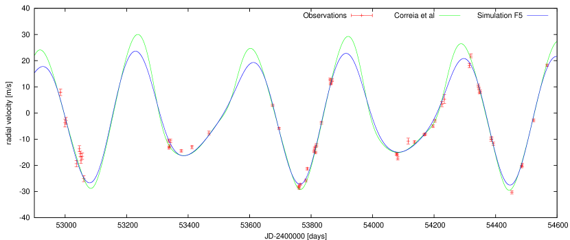
We can safely assume that the planet masses and periods are measured with high accuracy and that only the shape of the orbit contains large errors. Our best fit results in an unreduced value of . According to the above discussion, this solution is statistically indistinguishable from a solution with .
It is possible to reduce the value of even further, when assuming that the planet masses are not fixed. In that case, we have found a fit corresponding to where we have reduced the radial velocity amplitude by (effectively adding one free parameter to the fit). This could be explained by either a heavier star, less massive planets, or a less inclined orbit. The orientation of the orbital plane has been kept fixed () in all fits.
The results are shown in figure 8. The blue curve corresponds to the outcome of simulation F5 and we list the orbital parameters in table 2. We also plot the best fit given by Correia et al. (2008) for comparison (green curve). In accordance with the discussion given above, it is very difficult to see any differences in the quality of these fits, which indeed suggests that the models are statistically indistinguishable.
However, there is an important difference between the fits obtained from our simulations and that of Correia et al. (2008). Our models consistently predict lower values for both eccentricities and (see table 2). Furthermore, the ratio of eccentricities is higher than the previously reported value of . The eccentricities are oscillating and the ratio is on average .
This in turn results in a different libration pattern: the slow libration mode (see figure 3a in Correia et al., 2008) that is associated with oscillations of the angle between the two apsidal lines is absent, as shown in figure 10. Thus there is a marked difference in the form the interaction between the two planets takes place.
It is hoped that future observations will be able to resolve this issue. The evolution of the difference in radial velocity over the next few years between our fit from simulation F5 and the fit found by Correia et al. (2008) is plotted in figure 9. There is approximately one window each year that will allow further observations to distinguish easily between the two models. The large difference at these dates is not caused by the secular evolution of the system, but is simply a consequence of smaller eccentricities.


All runs that yield a final configuration with a 3:2 MMR are very similar in their dynamical behaviour, as found for model F5. They are characterised by an antisymmetric () state with a relatively small libration of and . This is a generic outcome of all convergent disc-planet migration scenarios that we performed.
6 Conclusions
The planets in the multi-planetary system HD45364 are most likely in a 3:2 mean motion resonance. This poses interesting questions on its formation history. Assuming that the planets form far apart and migrate with a moderate migration rate, as predicted by standard planet formation and migration theories, the most likely outcome is a 2:1 mean motion resonance, contrary to the observation of a 3:2 MMR.
In this chapter, we investigated a possible way around this problem by letting the outer planet undergo a rapid inward type III migration. We presented an analytical estimate of the required migration rate and performed both N-body and hydrodynamical simulations.
We find that it is indeed possible to form a 3:2 MMR and avoid the 2:1 resonance, thus resembling the observed planetary system using reasonable disc parameters. Hydrodynamical simulations suggest that the system is more likely to sustain the resonance for high aspect ratios, as the migration of the inner planet is slowed down, thus avoiding divergent migration.
Finally, we used the orbital configuration found in the hydrodynamical formation scenario to calculate a radial velocity curve. This curve was then compared to observations and the resulting fit has an identical value to the previously reported best fit.
Our solution is stable for at least a million years. It is in a dynamically different state, both planets having lower eccentricities and a different libration pattern. This is the first time that planet migration theory can predict a precise orbital configuration of a multiplanetary system. This might also be the first direct evidence for type III migration if this scenario turns out to be true.
The system HD45364 remains an interesting object for observers, as the differences between the two orbital solutions can be measured in radial velocity within a couple of years.
Chapter 4 The survival of mean motion resonances in a turbulent disc
Every body continues in its state of rest, or of uniform motion in a right line, unless it is compelled to change that state by forces impressed upon it.
Isaac Newton, Principia Mathematica, 1687
As shown for the system HD45364 in chapter 3, resonant configurations can be established as a result of dissipative forces acting on the planets which lead to convergent migration. The previous chapter assumes a laminar disc. However, in general the disc is thought to be turbulent because, as discussed in more detail in chapter 2, the molecular viscosity is not large enough to drive the observed outward angular momentum flux. The most promising mechanism to drive turbulence is the magneto-rotational instability, MRI (Balbus & Hawley, 1991), although other possibilities are still being discussed (see e.g. Lesur & Papaloizou, 2009).
In this chapter, we study the effects of density perturbations in the disc resulting from any kind of turbulence on planetary systems. We do not solve the full 3D magneto hydrodynamics equations, but rather assume a parametrisation for the forces acting on planets. This has two main advantages. First, we can understand the relevant dynamical processes much more easily. Second, there is a large diversity of simulations of the MRI in the literature which exhibit different diffusion coefficients, varying by several orders of magnitude. By parametrising the forces, we avoid these difficulties altogether.
Using this approach, we study the response of both a single planet and planetary systems in a 2:1 mean motion commensurability to stochastic forcing. The forcing could for example result from MRI turbulence. We first develop an analytic model from first principles. We can isolate two distinct libration modes for the resonant angles which react differently to stochastic forcing.
Systems are quickly destabilised if the magnitude of the stochastic forcing is large. The growth of libration amplitudes is parametrised as a function of the diffusion coefficient and other relevant physical parameters. We also perform numerical N-body simulations with additional stochastic forcing terms to represent the effects of disc turbulence. These are in excellent agreement with the analytic model.
Stochastic forcing due to disc turbulence may have played a role in shaping the configurations of observed systems in mean motion resonance. It naturally provides a mechanism for accounting for the HD128311 system, for which the fast mode librates and the slow mode is apparently near the borderline between libration and circulation.
1 Basic equations
We begin by writing down the equations of motion for a single planet moving in a fixed plane under a general Hamiltonian in the form (see e.g. Snellgrove et al., 2001; Papaloizou, 2003)
| (1) | |||||
| (2) | |||||
| (3) | |||||
| (4) |
Here the angular momentum of the planet is and the energy is . For a Keplerian orbital motion around a central point mass we have
| (5) | |||||
| (6) |
where is the gravitational constant, the semi-major axis and the eccentricity (see appendix 8). For an elliptical orbit around a point mass, equation 3 results in a linear growth of the mean longitude
| (7) |
where is the mean motion, being the time of periastron passage and being the longitude of periastron. All other equations of motion are trivial as the right hand side equates to zero.
1 Additional forcing of a single planet
In order to study phenomena such as stochastic forcing, we need to consider the effects of an additional external force per unit mass , which may or may not be described using a Hamiltonian formalism. However, as may be seen by considering general coordinate transformations starting from a Cartesian representation, the equations of motion are linear in the components of . Because of this we may determine them by considering forces of the form for which the Cartesian components are constant. Having done this we may then suppose that these vary with coordinates and time in an arbitrary manner. Following this procedure we note that when as in the above form is constant, we can derive the equations of motion by replacing the original Hamiltonian with a new Hamiltonian defined through
| (8) |
The additional terms proportional to the components of correspond to the Gaussian form of the equations of motion (Brouwer & Clemence, 1961).
The various derivatives involving can be calculated by elementary means and expressed in terms of and One thus finds additional contributions to the equations of motion 1 - 4, indicated with a subscript in the form
| (9) | |||||
| (10) | |||||
| (11) | |||||
| (12) | |||||
| (13) |
where the true anomaly is defined as the difference between the true longitude and the longitude of periastron, (see also appendix 8). Note that from equation 10 we obtain
| (14) |
and from equation 9 together with equation 10 we obtain
| (15) |
In the limit this becomes (ignoring terms and smaller)
| (16) |
Furthermore in this limit we may replace by
Note that that the above formalism results in equation 12 for , which diverges for small as . This comes from the choice of coordinates used and is not associated with any actual singularity or instability in the system. This is readily seen if one uses and as dynamical variables rather than and . The former set behave like Cartesian coordinates, while the latter set are the corresponding cylindrical polar coordinates. When the former set is used, potentially divergent terms do not appear. This can be seen from equations 12 and 16 which give in the small limit
| (17) | |||||
| (18) |
Abrupt changes to may occur when and pass through the origin in the plane. But this is clearly just a coordinate singularity rather than a problem with the physical system which changes smoothly on transition through the origin. The abrupt changes to the coordinate occur because very small perturbations to very nearly circular orbits produce large changes to this angle.
2 Multiple planets
Up to now we have considered a single planet. We now generalise the formalism so that it applies to a system of two planets. We follow closely the discussions in Papaloizou (2003) and Papaloizou & Szuszkiewicz (2005). Excluding stochastic forcing for the time being, we start from the Hamiltonian formalism describing their mutual interactions using Jacobi coordinates (Sinclair, 1975). In this formalism the motion of the outer planet is described around the centre of mass of the star plus the inner planet rather then the star alone. Thus, the radius vector of the inner planet of mass is measured from the star with mass and that of the outer planet, of mass is referred to the centre of mass of and . The reduced masses of and are then defined as and . We also define and . From now on we consistently adopt subscripts and for coordinates related to the outer and inner planets respectively. Note that this is different from the previous chapter.
The required Hamiltonian, is given by (Murray & Dermott, 2000, p.440ff):
| (19) |
Here is the relative position vector between the objects with subscript and , where 0 denotes the star. The Hamiltonian can be expressed in terms of and the time . The energies are given by and the angular momenta with and denoting the semi-major axes and eccentricities respectively. The mean motions are . As , we replace by and by from now on.
The interaction Hamiltonian (the term in equation 19) can be expanded in a Fourier series involving linear combinations of the three angular differences and (e.g. Brouwer & Clemence, 1961). Near a first order resonance, we expect that both and will be slowly varying. Following standard practice (see e.g. Papaloizou, 2003; Papaloizou & Szuszkiewicz, 2005) only terms in the Fourier expansion involving linear combinations of and as argument are retained because only these are expected to lead to large long term perturbations.
The resulting Hamiltonian may then be written in the general form where the interaction Hamiltonian is given by
| (20) |
where in the above and similar summations below, the sum ranges over all positive and negative integers and the dimensionless coefficients depend on and the ratio of semi-major axes only.
Equations of motion for two planets
The equations of motion for each planet can now be easily derived, that take into account the contributions due to their mutual interactions (see Papaloizou, 2003; Papaloizou & Szuszkiewicz, 2005) and contributions from 9 - 13. The latter terms arising from external forcing are indicated with a subscript . We obtain to lowest order in the perturbing masses:
| (21) | |||||
| (22) |
| (24) | |||||
| (25) | |||||
| (26) |
Here
| (27) | |||||
| (28) | |||||
and
| (29) | |||||
Note that is the angle between the two apsidal lines of the two planets. We also comment that, up to now, we have not assumed that the eccentricities are small and that, in addition to stochastic contributions, the external forcing terms may in general contain contributions from very slowly varying disc tides.
Modes of libration
We first consider two planets in resonance with no external forces, to identify the possible libration modes. In the absence of external forces, equations 21 - 26 can have a solution for which and are constants and the angles and are zero. In general, other values for the angles may be possible but such cases do not occur for the numerical examples presented below. When the angles are zero, equations 25 and 26 provide a relationship between and (see e.g. Papaloizou, 2003).
We go on to consider small amplitude oscillations or librations of the angles about their equilibrium state. Because two planets are involved there are two modes of oscillation, which we find convenient to separate and describe as fast and slow modes. Assuming the planets have comparable masses, the fast mode has a libration frequency and the slow mode has a libration frequency . These modes clearly separate as the planet masses are changed while maintaining fixed eccentricities.
Fast mode
To obtain the fast mode we linearise equations 21 - 26 and neglect second order terms in the planet masses. This is equivalent to neglecting the variation of and in equations 25 and 26 which then require that very nearly for this mode. Noting that for linear modes of the type considered here and in the next section, equations 21 - 24 imply that and are proportional to linear combinations of the librating angles, differentiation of either of equations 25 or 26 with respect to time then gives for small amplitude oscillations
| (30) |
where
| (31) |
and we have used the resonance condition that which is satisfied to within a correction of order . Note that for this mode the fact that very nearly, implies that is small. Thus that quantity does not participate in the oscillation.
Slow mode
Now, we look for low frequency librations with frequency . Equations 25 and 26 imply that, for such oscillations, to within a small relative error of order , throughout.
Equations 21 and 22 then imply that the two angles are related by , where . Subtracting equation 26 from equation 25, differentiating with respect to time and using this condition results in an equation for
| (32) |
where
| (33) |
with
and
Although the expressions for the mode frequencies are complicated, the fast frequency scales as the square root of the planet mass and the slow frequency scales as the planet mass. Both frequencies scale with the characteristic mean motion of the system.
Librations with external forcing
When external forcing is included source terms appear on the right hand sides of equations 30 and 32. We assume that the forcing terms are small so that terms involving products of these and both the libration amplitudes and the planet masses may be neglected. Then, in the case of the slow mode, repeating the derivation given above including the forcing terms, we find that equation 32 becomes
| (34) |
The quantities are readily obtained for each planet from equation 12. From this we see that for small eccentricities, , indicating large effects when is small. As already discussed, this feature arises from a coordinate singularity rather than physically significant changes to the system.
A similar description may be found for the fast mode. In this case, neglecting terms of the order of the square of the planet masses or higher, one may use equations 25 and 26 to obtain an equation for in the form
| (35) |
Equations 35 and 34 form a pair of equations for the stochastically forced fast and slow modes respectively. This mode separation is not precise. However, it can be made so by choosing appropriate linear combinations of the above modes. Numerical results confirm that predominantly manifests the fast mode and the slow mode, so we do not expect such a change of basis to significantly affect conclusions.
We further comment that because contains but not , for small eccentricities there are only potential forcing terms that occur when forcing is applied to the inner planet. As this planet has the larger eccentricity for the situations we consider, small eccentricities are not found to play any significant role in this case.
Each mode responds as a forced oscillator. The forcing contains a stochastic component which tends to excite the respective oscillator and ultimately convert libration into circulation. But we stress that the above formulation as well as developments below assume small librations, so we may only assess the initial growth of oscillation amplitude. However, inferences based on the structure of the non linear governing equations and an extrapolation of the linear results enable successful comparison with numerical results.
3 Stochastic forces
We assume that turbulence causes the external force per unit mass acting on each planet to be stochastic. For simplicity we shall adopt the simplest possible model. Each component of the force satisfies the relation
| (36) |
where the auto-correlation function is such that , where is the correlation time and is the root mean square value of the component. Note that an ensemble average is implied on the left hand side. Again, for simplicity we assume that different components acting on the same planet as well as components acting on different planets are uncorrelated. The root mean square values as well as may in general depend on , but we shall not take this into account here and simply assume that these quantities are constant and the same for each force component.
The stochastic forces make quantities they act on undergo a random walk. Thus, if for example for some quantity111Constants or slowly varying quantities originally multiplying may be absorbed by a redefinition of and so do not affect the discussion given below. , the square of the change of occurring after a time interval is given by
| (37) | |||||
Here we take the limit where is very large corresponding to an integration time of many correlation times and is the diffusion coefficient.
When the evolution of a stochastically forced planetary orbit is considered, it is more appropriate to consider a model governing equation for of the generic form
| (38) |
where we recall that is the orbital period (but note that a different value could equally well be considered). We note in passing that, by shifting the origin of time, an arbitrary phase may be added to the argument without changing the results given below. One readily finds that equation 37 is replaced by
| (39) | |||||
where we introduce a new correction factor . If , corresponding to the correlation time being much less than the orbital period, then . For larger gives a reduction factor for the amount of stochastic diffusion. For example if we adopt, an exponential form for the auto-correlation function such that
we find
| (40) |
and for the purposes of simplicity and comparison with numerical work we shall use this from now on.
Stochastic forcing of an isolated planet
In the case of a stochastically forced single planet we may obtain a statistical estimate for the characteristic growth of the orbital parameters as a function of time by directly integrating equations 10, 12, 16, 17 and 18 with respect to time. We may then apply the formalism leading to the results expressed in generic form through equations 37 - 40 to obtain estimates for the stochastic diffusion of the orbital elements in the limit of small eccentricity in the form
| (41) | |||||
| (42) | |||||
| (43) | |||||
| (44) | |||||
| (45) | |||||
| (46) |
As mentioned before, the dependence of which arises from the coordinate singularity does not appear for and . Note that the definitions of and imply, consistently with the above, that
| (47) | |||||
| (48) |
The evolution of the longitude
Of special interest is also the evolution of the planet’s mean longitude. In observations of Saturn’s rings, for example, it is much easier to measure a shift of the longitude of an embedded moonlet compared to a direct measurement of the change in its semi-major axis. The time derivative of the mean motion is given by
| (49) |
Assuming a nearly circular () orbit, the mean longitude is thus given by the double integral
| (50) | |||||
| (51) |
The root mean square of the difference compared to the unperturbed orbit is
| (52) | |||||
| (53) | |||||
| (54) | |||||
| (55) | |||||
| (56) |
where we have taken the limit of in the last line. We also assume an exponentially decaying auto-correlation function because the integral in equation 54 can not be solved analytically for an arbitrary function . Note that on short timescales, other terms in equation 56 may dominate the growth of .
Instead of a stochastic migration, let us also assume a laminar migration with constant migration rate , given by
| (57) |
As above, we can calculate the longitude as a function of time as the following double integral
| (58) | |||||
| (59) |
and thus
| (60) |
Note that equation 60 is an exact solution, whereas equation 56 is a statistical quantity, describing the root mean square value in an ensemble average. In the stochastic and laminar case, grows like and , respectively. This allows to discriminate the different mechanisms by observing over an extended period of time.
Stochastic variation of the resonant angles in the two planet case
We now consider the effects of stochastic forcing on the resonant angles. The expressions are more complicated than in the previous section because there are more variables involved. However, we basically follow the same formalism.
While the libration amplitude is small enough for linearisation to be reasonable, the evolution is described by equations 34 and 35. These may be solved by the method of variation of parameters. Assuming the amplitude is zero at , the solution of equation 34 is given by
| (61) |
where . Equation 61 may be regarded as describing a harmonic oscillator whose amplitude varies in time such that the square of the amplitude after a time interval is given by
| (62) |
The corresponding expression for equation 35 is
| (63) |
where
We now evaluate the expectation values of these using the formalism of the previous section. For simplicity we specialise to the case when stochastic forces act only on the outer planet. This is also what has been considered numerically later. Taking equation 62, we perform an integration by parts, neglecting the end point contributions as these are sub-dominant (they increase less rapidly than for large ), to obtain
| (64) |
In dealing with equation 63 we neglect in because after integration by parts this leads to a contribution on the order smaller than that derived from . Thus, we simply obtain
We again follow the procedures outlined in the previous section to obtain the final growth estimates
| (65) | |||||
| (66) |
where the corrections factors are given by
| (67) | |||||
| (68) |
The correction factors and compare the relevant timescales of the system (here, the libration periods) to the correlation time of the stochastic force.
Growth of libration amplitudes
Equations 65 and 66 express the expected growth of the resonant angle libration amplitudes as a function of time. These expressions can be simply related to those obtained for a single planet. Thus equations 41 and 66 applied to the outer planet imply that
As we are interested in the case , the width of the libration zone is , we see that the time for to reach unity is comparable for the semi-major axis to diffuse through the libration zone.
For fixed eccentricity of the inner planet , equation 65 indicates that , being the angle between the apsidal lines of the two planets, diffuses in the same way as for an isolated outer planet subject to stochastic forces. Thus, in the small amplitude regime, the way this diffusion occurs would appear to be essentially independent of whether the planets are in resonance.
An important consequence of equation 65 is the behaviour of for small . The latter quantity was assumed constant in the analysis. As already discussed earlier, abrupt changes to are expected when the eccentricity of one planet gets very small. Then, even an initially small amplitude libration is converted to circulation. Thus if is small, then equation 65 indicates that a time , is required to convert libration to circulation. This can be small if is small. Even if is not small initially, it is important to note that it also undergoes stochastic diffusion (see equation 43) as well as oscillations through its participation in libration. Should attain very small values through this process, then from equation 65 we expect the onset of a rapid evolution of . This is particularly important when already starts from relatively small values.
In fact, application of equations 65 and 66 to the numerical examples discussed below, adopting the initial orbital elements, indicate that the diffusion of is significantly smaller than unless starts out with a very small value. This would suggest that reaches circulation before . However, this neglects the coupling between the angles that occurs once the libration amplitudes become significant. It is readily seen that it is not expected that could circulate while remains librating as it was initially. One expects to recover standard secular dynamics for from the governing equations 21 - 25, when these are averaged over an assumed circulating with constant . As a libration of the initial form would not occur under those conditions, we expect, and find, large excursions or increases in the libration amplitude of to be correlated with increases in the libration amplitude of . This in turn increases the oscillation amplitude of the eccentricity , allowing it to approach zero. The consequent rapid evolution of then enables it to pass to circulation. Thus, the breaking of resonance is ultimately found to be controlled by the excitation of large amplitude librations for , which induce to pass to circulation somewhat before itself.
2 Numerical simulations
We have performed numerical simulations of one and two planet systems that allow for the incorporation of additional stochastic forces with the properties described above. These forces provide a simple prescription for estimating the effects of stochastic gravitational forces produced by density fluctuations associated with disc turbulence. The results have been obtained using the N-body code described in chapter 3. We have checked that results are converged and do not depend on the integrator used.
We first discuss the expected scaling of the stochastic forces with the physical parameters of the disc and their implementation in N-body integrations. In order to clarify the physical mechanisms involved, and to check the analytic predictions for stochastic diffusion given by equations 41 - 45, we consider simulations of a single planet undergoing stochastic forcing first. We then move on to consider two planet systems with and without stochastic forcing. We focus on the way a 2:1 commensurability is disrupted and highlight the various evolutionary stages a system goes through as it evolves from a state with a strong commensurability affecting the interaction dynamics, to one where the commensurability is completely disrupted. We find that in some cases a strong scattering occurs. We consider a range of different planet masses and eccentricities (see table 1).
1 Stochastic forces
In order to mimic the effects of turbulence, for example produced by the MRI, it is necessary to calibrate these forces with reference to MHD simulations. As described above, the basic parameters characterising the prescription for stochastic forcing that we have implemented are the root mean square value of the force components per unit mass (in cylindrical coordinates) and the auto correlation time .
From our analytic considerations, we conclude that stochastic forces make the orbital parameters undergo a random walk that is dependent on the force model primarily through the diffusion coefficient but also through the dimensionless correction factors and .
For planets under the gravitational influence of a proto-planetary disc, the natural scale for the force per unit mass components, , is , where is the characteristic disc surface density (see e.g. Papaloizou & Terquem, 2006). is the gravitational force per unit mass due to a small circular disc patch of radius at a distance from its centre assuming that all its mass is concentrated there. See also figure 1. This is independent of . The natural correlation time is the inverse of the orbital angular frequency . We adopt a minimum mass solar nebula model (MMSN, see Weidenschilling, 1977b) with
| (69) |
This provides a natural scale for as a function of the local disc radius and the central stellar mass through222The scaling in Rein & Papaloizou (2009) is incorrect due to a missing factor of . The value in this thesis has been corrected.
| (70) |
where is a dimensionless constant. There are several factors which contribute to the value of :
-
•
The density fluctuations found in MRI simulations are typically of the order (e.g. Nelson, 2005).
-
•
The presence of a dead zone in the mid plane regions of the disc, where the MRI is not active, has been found to cause reductions in the magnitude of by one order of magnitude or more, as compared to active cases (Oishi et al., 2007).
-
•
Massive planets open a gap in the disc. Oishi et al. (2007) found that most of the contribution to the stochastic force comes from density fluctuations within a distance of one scale-height from the planet. When a gap forms, this region is cleared of material leading to a substantial decrease in the magnitude of turbulent density fluctuations. Consequently should be reduced on account of a lower ambient surface density. A factor of seems reasonable, although it might be even smaller (de Val-Borro et al., 2006).
- •
If it is appropriate to include reduction factors to account for all of the above effects, one finds and we expect a natural scale for the diffusion coefficient to be specified through
| (71) |
The same value of D may be equivalently scaled to the orbital parameters of the planets without reference to the disc by writing
| (72) |
Thus, a value in cgs units corresponds to a ratio of the root mean square stochastic force component to that due to the central star of about for a central solar mass at AU. It is a simple matter to scale to other locations.
Of course we emphasise that the value of this quantity is very uncertain, a situation that is exacerbated by its proportionality to the square of the magnitude of the stochastic force per unit mass. For this reason we perform simulations for a range of , covering many orders of magnitude.
| Planet | () | (AU) | (days) | ||
|---|---|---|---|---|---|
| GJ876 c | 0.790 | 0.131 | 30.46 | 0.263 | |
| b | 2.530 | 0.208 | 60.83 | 0.031 | |
| GJ876 LM c | 0.13 | 0.131 | 30.46 | 0.263 | |
| b | 0.42 | 0.208 | 60.83 | 0.031 | |
| GJ876 SE c | 0.013 | 0.131 | 30.46 | 0.263 | |
| b | 0.042 | 0.208 | 60.83 | 0.031 | |
| GJ876 E c | 0.0013 | 0.0131 | 30.46 | 0.263 | |
| b | 0.0042 | 0.208 | 60.83 | 0.031 | |
| GJ876 LM HE c | 0.13 | 0.131 | 30.46 | 0.41 | |
| b | 0.42 | 0.208 | 60.83 | 0.09 | |
| GJ876 SE HE c | 0.013 | 0.131 | 30.46 | 0.41 | |
| b | 0.042 | 0.208 | 60.83 | 0.09 | |
| HD128311 b | 1.56 | 1.109 | 476.8 | 0.38 | |
| c | 3.08 | 1.735 | 933.1 | 0.21 |
2 Numerical implementation of correlated noise
The procedure we implemented, uses a discrete first order Markov process to generate a correlated, continuous noise that is added as an additional force. This statistical process is defined by two parameters, the root mean square of the amplitude and the correlation time (Kasdin, 1995). It has a zero mean value and has no memory. This has the advantage that previous values do not need to be stored in memory. The auto-correlation function decays exponentially and thus mimics the auto-correlation function measured in MHD simulations by Oishi et al. (2007). It is also consistent with the assumptions made in the previous sections.
The procedure for generating noise in a variable x with an auto-correlation time tau and root mean square value of 1 is as follows. The update of x from t to t+dt in pseudo code is
x *= exp( -dt / tau)
x += Xi * sqrt( 1 - exp( 2 * dt / tau ) )
where Xi is a random variable with normal distribution and a variance of unity.
3 Stochastic forces acting on a single planet


We first investigate the long-term effect of stochastic forces on a single isolated planet. The initial orbital parameters are taken to be the observed parameters of GJ876 b (see table 1). In this simulation, we use the reduced diffusion coefficients
which can be represented by a correlation time of half the orbital period and a specific force with root mean square values , and , respectively (see also equation 72). In that case the correction factor evaluates to .
The growth rates of the root mean square values for , and in 200 simulations are plotted in figure 2. We also plot the analytic predictions (equations 41, 45 and 43) as solid lines. The numerical simulations and the analytic model are in excellent agreement and scale as expected. We have performed simulations for a variety of diffusion coefficients and get results that are fully consistent in all cases.
We also plot the analytic growth rates coming from equations 45 and 43 while setting , which corresponds to uncorrelated noise. The resulting curves (dashed lines) do not agree with simulation results. This shows clearly that correlation effects are important, and have to be taken into account. The model presented by Adams et al. (2008) makes use of such an uncorrelated force (random kicks), leading to an overestimated diffusion coefficient by almost a factor . Note that only orbital parameters involving the geometry of the orbit are affected, i.e., not the semi-major axis.
4 Illustration of the modes of libration in a two planet system
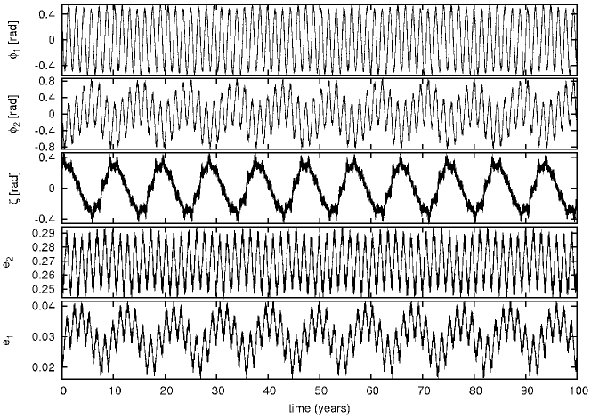
We now go on to consider two planet systems. As an illustrative example we discuss the GJ876 system (see table 1). We begin by considering the evolution of the system without stochastic forcing in order to characterise the modes of libration of the resonant angles and other orbital parameters. In particular, we identify the fast and slow modes discussed in section 2.
The time evolution of the resonant angles and the eccentricities of the unperturbed system is plotted in figure 4. Clearly visible are the slow and fast oscillation modes. The fast mode, which is seen to have a period of about 1.4 years, dominates the librations of and while also being present in those of . On the other hand the slow mode, which is seen to have a period of about 10 years, dominates the librations of while also being present in those of and
We emphasise the fact that the eccentricities of the two planets participate in the librations, and are therefore not constant. In particular, the eccentricity of GJ876 b oscillates around a mean value of with an amplitude . This behaviour involving the attainment of smaller values of the eccentricity has important consequences for stochastic evolution as discussed above (section 3) and also below.
We remark that similar behaviour occurs for all the systems we have studied, these having a wide range of eccentricities and planet masses. The fast and slow mode periods scale with the planet masses as given by equations 31 and 33 respectively. These indicate, as confirmed by our simulations, that if both masses are reduced by a factor then the period of the fast mode scales as and the period of the slow mode scales as

In figure 5 we plot the librations in and variables. The left plots show one period of the slow mode libration, corresponding to one complete circle around the origin. Super-imposed on that are slow mode librations with higher frequency. The frequency ratio is , thus the hexagon shape. The even higher frequency modes correspond to the orbital period itself. The right plots show many libration periods.
3 Two planets with stochastic forcing
We now consider systems of two planets with stochastic forcing. For simplicity we begin by applying additional forces only to the outer planet. We have found that adding the same form of forcing to the inner planet tends to speed up the evolution by approximately a factor of two without changing qualitative details. For illustrative purposes we again start with the GJ876 system and consider two diffusion coefficients and . In all of our simulations a constant value of is used by maintaining both parameters and constant. For the cases considered here, there is little orbital migration so that this effect can be ignored.
The time evolution of the eccentricities is plotted for two runs in the first and third plot in figure 6. We see fast oscillations superimposed on a random walk. The amplitude of the oscillations, as well as the mean value, change with time.
Our simple analytic model assumes slowly changing background eccentricities and semi-major axes. Accordingly, it does not incorporate the oscillations of the eccentricity due to the resonant interaction of the planets. In order to make a comparison, we perform a time average over many periods to get smoothed quantities whose behaviour we can compare with that expected from equations 41 - 45. When this procedure is followed (see second and forth plot in figure 6), the evolution is in reasonable accord with that expected from the analytic model provided that allowance is made for the importance of small values of in determining the growth of the libration amplitude of the angle between the apsidal lines of the two planets (see equation 45). The presence of this feature results in the behaviour of the libration amplitude being more complex than that implied by a process governed by a simple diffusive random walk. This is discussed in the following sections.
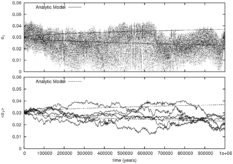
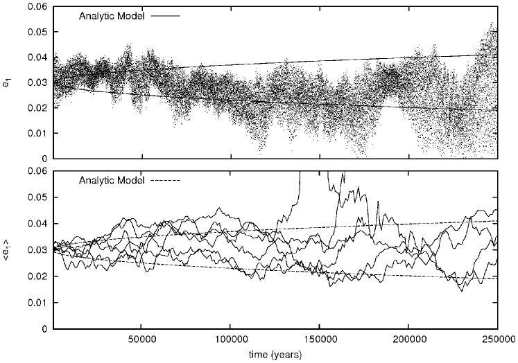
1 Disruption of a resonance in stages
Systems with mean motion commensurabilities can be in many different configurations. Here we describe the important evolutionary stages as they appear in a stochastically forced system starting from a situation in which all the resonant angles show small amplitude libration. Observations of GJ876 suggest that the system is currently in such a state with the ratio of the orbital periods oscillating about a mean value of
Attainment of circulation of the angle between the apsidal lines
When the initial eccentricity of the outer planet, , is small, the excitation of the libration amplitudes of the resonant angles readily brings about a situation where attains even smaller values. This then causes the periastron difference to undergo large oscillations and eventually reach circulation (see equation 45). Should stochastic forces cause to reach zero, on account of the coordinate singularity, becomes undefined. Note that this occurs without a large physical perturbation to the system. Thus, the occurrence of this phenomenon does not imply the system ceases to be in a commensurability.
In this context we note that the eccentricity of GJ876 b initially is such that with values often being attained during libration cycles. Thus only a small change may cause the above situation to occur. In all cases that we have considered, we find that enters circulation prior to the fast angle , which may remain librating until that too is driven into circulation.
Attainment of circulation of the fast angle
Both before and after enters circulation, stochastic forces increase the libration amplitude of the fast mode . This mode dominates both the librations of the resonant angle and the semi-major axes. Eventually starts circulation. Shortly afterwards, commensurability is lost and starts to undergo a random walk with a centre that drifts away from 2. Note that it is possible for some realisations to re-enter commensurability. For systems with the masses of the observed GJ876 system, the most likely outcome is a scattering event that causes complete disruption of the system.

Because the eccentricities do not play an important role in the attainment of circulation of the fast angle, we can use equation 66 to calculate the growth rate. The root mean square values of as a function of time, taken from both, analytical and numerical results, are plotted in figure 7. Here, we use . Note that as mentioned above, is circulating first (in the presented case this happens after years). However, this does not influence the growth of .
2 A numerical illustration
In order to illustrate the evolutionary sequence described above we plot results for two realisations of the evolution of the GJ876 system in figure 8. For these runs we adopted the diffusion coefficient . Note that increasing only decreases the evolutionary time which has been found, both analytically and numerically to be (see below).
The times at which the transition from libration to circulation occurs for both the slow and fast angles, are indicated by the vertical lines in figure 8.
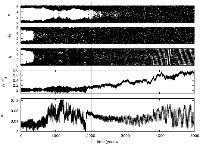
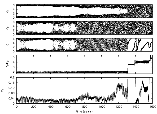
Several of the features discussed above and in section 3 can be seen in figure 8. In particular the tendency for the occurrence of very small values of to be associated with transitions to circulation of can be seen for the realisation plotted in the lower panels at around years and years. Such episodes always seem to occur when the libration amplitude of the fast angle is relatively boosted, indicating that this plays a role in boosting the slow angle. If the duration for which attains small values is small and recovers small amplitude librations, the slow angle returns to circulation. Thus, the attainment of long period circulation for the slow angle is related to the diffusion time for . We also see from figure 8 that the angle , which has a large contribution from the slow mode, behaves in the same way as as far as libration/circularisation is concerned. We have verified by considering the results from the simulations of GJ876 LM HE, which started with a larger value of that, as expected, the attainment of circulation of the slow angle takes relatively longer in this case, the time approaching more closely the time when attains circulation. Also as expected, the time when attains circulation is not affected by the change in .
3 Dependence on the diffusion coefficient
We now consider the stability of the systems listed in table 1 as a function of . These systems have a variety of masses and orbital eccentricities. In particular, in view of the complex interaction between the resonant angles discussed above, we wish to investigate whether the mean amplitude growth at a given time is indeed proportional to . As also mentioned above, the value of the diffusion parameter that should be adopted, is very uncertain. We have therefore considered values of ranging over five orders of magnitude. The correlation time is always taken to be given by while the RMS value of the force is changed. In order to determine the lifetime of a resonant angle, we monitor whether it is librating or circulating. Numerically, libration is defined to cease when the angle is first seen to reach absolute values larger than . We note that the angle can in general regain small values afterwards. However, this is a transient effect and changes the lifetime by no more than a factor of in all our simulations.
In this context we consider the fast angle and the slow angle . As we saw above, the latter can be replaced by which exhibits the same behaviour. Because is the last to start circulating, the resonance is defined to be broken at that point.
Equations 66 and 65 estimate the spreading of the resonant angles as a function of time. We plot both the numerical and analytical results in figure 9. To remove statistical fluctuations and obtain a mean spreading time, the numerical values for a particular value of were obtained by averaging over realisations.
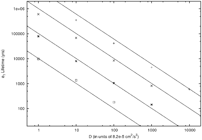
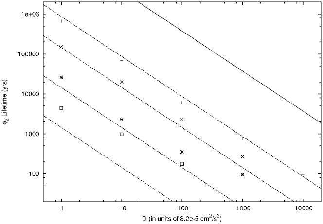
From figure 9 it is apparent that the evolutionary times scale is for varying by many orders of magnitude. The analytic estimates for the libration survival times of , dominated by the fast mode, obtained using equation 66 adopting the initial orbital elements and with the fast libration frequency determined from the simulations, are plotted in the upper panel of figure 9. These are in good agreement with the numerical results. However, the estimate for based on equation 65 using the initial value of overestimates the lifetime by a factor of at least (see solid line in the lower plot of figure 9). Furthermore equation 65 has no dependence on planet mass which is in clear conflict with the numerical results. As discussed above, this is due to the temporary attainment of small eccentricities. This causes the disruption of the libration of earlier than predicted assuming being constant. In fact this disruption occurs at times that can be up to times shorter than those required to disrupt . We estimate the lifetime of librations of by calculating the time needs to reach values close to (see dashed lines in the lower plot of figure 9). As explained above in section 3, large amplitude variations of are expected to couple to and excite the slow mode. Variations induced in the eccentricity allow to reach zero and we lose libration of . These simple estimates are in good agreement with the numerical results and accordingly support the idea that and are indeed coupled in the non-linear regime. For low mass planets this simple analytic prediction underestimates the lifetime of by a factor of , suggesting that the coupling between the two modes depends slightly on the planet masses.
To confirm our understanding of these processes, we have repeated the calculations with systems that are in the same state as the system discussed above but have higher eccentricities (see GJ876 LM HE and GJ876 SE HE in table 1). The lifetime of the librating state of is unchanged, as this does not depend significantly on the eccentricity. However, the lifetime of the librating state of is a factor of longer. This is due to the fact that a larger excitation of is needed to make reach small values in these simulations.
The random walk description breaks down completely when the anticipated disruption time becomes shorter than the libration period. This is expected to happen for small enough masses as can be verified from figure 9. It is because the disruption time decreases linearly with the planet masses while the libration period increases as the square root of the planet masses. Then we cannot average over many libration periods. This situation is apparent in figure 9 for very short disruption times of the order 100-1000 years where survival times cease to vary linearly with .
4 Formation of HD128311
Having understood the effects of stochastic forces on resonances, we now go on to discuss the application of these ideas to the formation of the orbital configuration of the planetary system HD128311. This is (with 99% confidence) in a 2:1 mean motion resonance, with the angle librating and the angle circulating so that there is no apsidal co-rotation (Vogt et al., 2005). However, the orbital parameters are not well constrained. The original Keplerian fit by Vogt et al. (2005) is such that the planets undergo a close encounter after only 2000 years. The values in table 1 have been obtained from a fit to the observational data that includes interactions between the planets. The values quoted have large error bars. For example the eccentricities and have an uncertainty of 33% and 21%, respectively. Although the best fit doesn’t manifest apsidal co-rotation, the system could undergo large amplitude librations and still be stable.
According to Lee & Peale (2002) the planets should have apsidal co-rotation if the commensurability was formed by the two planets undergoing sufficiently slow convergent inward migration, and if they then both migrated inwards significantly while maintaining the commensurability (see also Snellgrove et al., 2001). Accordingly Sándor & Kley (2006) suggested a possible formation scenario with inward migration as described above, but with an additional perturbing event, such as a close encounter with an additional third planet occurring after the halting of the inward migration. This perturbation is needed to alter the behaviour of , so that it undergoes circulation rather than libration and thus producing orbital parameters similar to the observed ones.
We showed above that stochastic forcing possibly resulting from turbulence driven by the MRI readily produces systems with commensurabilities without apsidal co-rotation if the eccentricities are not too large. This suggests that a scenario that forms the commensurability through disc-induced inward convergent migration might readily produce commensurable systems without apsidal co-rotation if stochastic forcing is included. Such scenarios are investigated in this section.
We present simulations of the formation of HD128311 that include migration and stochastic forcing due to turbulence but do not invoke artificial perturbation events involving additional planets. We find that model systems with orbital parameters resembling the observed ones are readily produced and are better matches than those provided by Sándor & Kley (2006). The planets in this system are of the order of several Jupiter masses and the eccentricity of one planet can get very small during one libration period. The observed orbital parameters are given in table 1 and their time evolution (due to planet-planet interactions) is plotted on the right hand side of figures 10, 11 and 12. The mass of the star is .
1 Migration forces
We incorporate the non-conservative forces exerted by a proto-stellar disc that lead to inward migration by following the approach outlined in appendix 9. The migration process is characterised by migration and eccentricity damping timescales, and , respectively. This procedure is now widely used (e.g. Sándor & Kley, 2006; Crida et al., 2008). We also use the ratio of the above timescales, , as defined in chapter 3. This ratio determines the eccentricities in the state of self-similar inward migration of the commensurable system that is attained after large times.
In this work we allow the planets to form a commensurability through convergent inward migration with stochastic forcing included. The disc is then removed through having its surface density reduced to zero on a 2000 year timescale. This reduces both the migration forces and the stochastic forces simultaneously. This procedure is very similar to that adopted by the above authors but we have included stochastic forcing and removed the disc on longer, more realistic, time-scales.
The stochastic forces need to have the right balance with respect to the migration rate. We have found that inward migration imparts stability to the resonant system. If the migration rate is too fast relative to the stochastic forcing the migration keeps down the libration amplitudes and we do not get circulation. On the other hand large eccentricity damping favours broken apsidal co-rotation. This might look counter intuitive at first sight, but remember that the diffusion of depends on and .
Due to the stochastic nature of the problem, it is hard to present a continuum of solutions so we restrict ourselves to the discussion of three representative examples. However, we comment that we are able to obtain similar end states for a wide range of migration parameters.
As above, the parameters and are kept constant, so maintaining constant, for the duration of the simulation, with being determined for the initial location of the outer planet. As discussed above, these values may scale with the radius of the planet and we thus expect them to change during migration. However, the semi-major axis of the outer planet changes only by % during the simulation. Consequently, we ignore this effect.
2 Model 1

The planets are initially on circular orbits at radii AU and AU. Stochastic forcing is applied to the outer planet only, with a diffusion coefficient of . Note that although this value is 64 times larger than the scaling given by equation 71, corresponding to a force that is 8 times larger than the simple estimate given in section 1, corresponding to smaller reduction factors resulting from a gap or dead zone, it is too small for the angle to be brought to circulation during our runs. The results given above and summarised in figure 9, and further tests, indicate that similar results would be obtained if is reduced, but on a longer time-scale provided the migration rate is also ultimately reduced appropriately so that the system can survive for long enough to enable to be driven into circulation.
The outer planet is made to migrate inwards on a timescale years. The inner planet migrates slowly outwards on a timescale of years. This results in convergent migration. For both planets we use an eccentricity to semi-major axis damping ratio of . The resulting evolutionary timescales are significantly larger than those used by Sándor & Kley (2006) and more easily justified by hydrodynamical simulations.
The time evolution is shown in the left plot of figure 10. After resonance capturing all angles are either initially librating or on the border between libration and circulation. The slow mode has a period of years, whereas the fast mode period is 20 times shorter.
It can be seen from figure 10 and other similar figures below, that while migration continues, libration amplitudes tend to be controlled apart from when becomes either zero or very close to zero. Then, due to stochastic forcing, and start circulating. Subsequently, libration is recovered over time intervals for which does not attain very small values but eventually additional stochastic forcing together with the repeated attainment of small values for causes to remain circulating for the remainder of the simulation. After years, both the forces due to migration and turbulence are reduced smoothly on a timescale of years. The result is a stable configuration that resembles the observed system very well.
3 Model 2
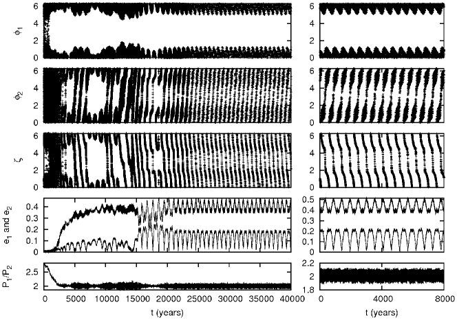
For this simulation, we lengthen the migration timescales by a factor of 2 to show that the results are generic. We also decrease the value of to . All other parameters are the same as for model 1. This results in larger eccentricities and the final state better resembled our representation of the observed system. However, it should be kept in mind that the eccentricities are not well constrained by the observations.
The time evolution is plotted in figure 11. The resonant angles librate immediately after the capture into resonance, as predicted for sufficiently slow migration. However, in the same way as for model 1 described above, stochastic forces make circulate soon afterwards. Once the migration forces and stochastic forces are removed between and years, the system stays in a stable configuration with no apsidal co-rotation.
4 Model 3
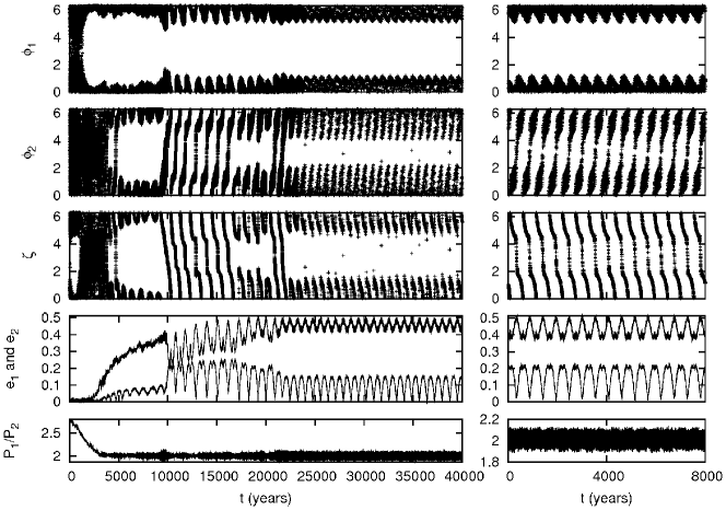
All parameters are the same as for model 2. Accordingly, model 3 represents another statistical realisation of that case. The time evolution is plotted in figure 12. The final state is very close to the boundary between libration and circulation of . As discussed above, large uncertainties in the orbital parameters mean that the actual system could be in such a state.
Due to stochastic forces, which may result from local turbulence, we are able to generate a broad spectrum of model systems. Some of them undergo a strong scattering during the migration process. However, the surviving systems resemble the observed system very well. Although the orbital parameters are not well constrained yet, we showed that values in the right range are naturally produced by a turbulent disc.
5 Conclusions
In this chapter, we have presented a self-consistent analytical model of both a single planet, and two planets in a mean motion resonance, being subject to external stochastic forcing. The stochastic forces could result from MRI-driven turbulence within the proto-planetary disc but our treatment is equally applicable to any other source, for example from a gravitoturbulent disc such as Saturn’s A-ring (see chapter 5).
We considered the evolution of a stochastically forced two planetary system that is initially deep inside a MMR (i.e., the two independent resonant angles librate with small amplitude). Stochastic forces cause libration amplitudes to increase in the mean with time until all resonant angles are eventually driven into circulation, at which point the commensurability is lost. Often a strong scattering occurs soon afterwards for systems composed of planets in the Jovian mass range.
We isolated a fast libration mode which is associated with oscillations of the semi-major axes and a slow libration mode which is mostly associated with the motion of the angle between the apsidal lines of the two planets. These modes respond differently to stochastic forcing, the slow mode being more readily converted to circulation than the fast mode. This slow mode is sensitive to the attainment of small eccentricities, which cause rapid transitions between libration and circulation. The amplitude of the fast mode grows more regularly in the mean, with the square of the libration amplitude in most cases increasing linearly with time and being proportional to the diffusion coefficient . Of course this discussion is simplified and there are limitations. For example if the total mass of the system is reduced, the disruption time eventually becomes comparable to the libration period. In that case the averaging process that we use in the derivation is no longer valid and the lifetime no longer scales as
The analytic model was compared to numerical simulations which incorporate stochastic forces. Those forces, parametrised by the mean square values of each component in cylindrical coordinates and the auto-correlation time, are applied in a continuous manner giving results that could be directly compared with the analytic model. The simulations are in broad agreement with analytic predictions and we presented illustrative examples of the disruption process. We performed the simulations for a large range of diffusion parameters, planet masses and initial eccentricities to verify the scaling law for the commensurability disruption time summarised hereafter.
To summarise our results, recalling that the slow angle is driven into circulation before the fast angle, so that the ultimate lifetime is determined by the time taken for the fast angle to achieve circulation, we determine the lifetime, , using equation 66, setting together with , we obtain
| (73) |
We showed above that this gives good agreement with our numerical results. Using we can express this result in terms of the relative magnitude of the stochastic forcing in the form
| (74) |
where is the orbital period of the outer planet. Here the first quantity in brackets represents the ratio of the square of the central force per unit mass to the mean square stochastic force per unit mass acting on the outer planet. The other quantities in brackets, scaled to the GJ876 system are expected to be unity, while the last factor is the ratio of the total mass ratio of the system to the same quantity for GJ876. Here, it is assumed that the two planets in the system have comparable masses.
From equation 74, we see that a non-migrating system such as GJ876 could survive in resonance for years if the stochastic force amplitude is times the central force. This expression enables scaling to other systems at other disc locations for other stochastic forcing amplitudes. Inference of survival probabilities for particular systems depends on many uncertain aspects, such as the proto-planetary disc model and the strength of the turbulence. However, the mass ratio dependence in equation 74 indicates that survival is favoured for more massive systems. At the present time the number of observed resonant systems is too small for definitive conclusions to be made. However, the fact that several systems exhibiting commensurabilities have been observed indicates that resonances are not always completely disrupted by stochastic forces due to turbulence, but rather may be modified as in our study of HD128311.
The most likely orbital configuration of the HD128311 system is such that the fast mode librates with the slow mode being near the borderline between libration and circulation. We found that such a configuration was readily produced in a scenario in which the commensurability was formed through a temporary period of convergent migration, with the addition of stochastic forcing. During a migration phase moderate adiabatic invariance applied to the libration modes together with eccentricity damping leads to increased stabilisation and a longer lifetime for the resonance. However, the time evolution of the eccentricity, and in particular the attainment of small values, plays an important role in causing the slow mode to circulate. This corresponds to the loss of apsidal co-rotation. Thus we expect that a large eccentricity damping rate does not necessarily stabilise the apsidal co-rotation of a system. Additional simulations have shown that this is lost more easily for large damping rates (). On the other hand, it should be noted that this has less significance when one of the orbits becomes nearly circular.
Further observations of extra-solar planetary systems leading to better statistics may lead to an improved situation for assessing the role of stochastic forcing.
Chapter 5 Stochastic migration of small bodies in Saturn’s rings
Have not the small particles of bodies certain powers, virtues, or forces, by which they act at a distance, not only upon the rays of light for reflecting, refracting, and inflecting them, but also upon one another for producing a great part of the Phenomena of nature?
Isaac Newton, Optiks, Query 31, 1729
In the previous chapter, we discussed the stochastic migration of planets, embedded in a circum-stellar disc. A very similar process also occurs in the circum-planetary disc known as Saturn’s rings. However, both the length and time scales involved are three orders of magnitude smaller. The bodies of interest are small moonlets. These sized bodies have been predicted both analytically and numerically (Spahn & Sremčević, 2000; Sremčević et al., 2002; Seiß et al., 2005). They create propeller shaped structures due to their disturbance of the rings and have been observed only recently by the Cassini spacecraft in the A and B ring (Tiscareno et al., 2006, 2008).
They can migrate within the rings, similar to proto-planets which migrate in a proto-stellar disc. Depending on the disc properties and the moonlet size, this can happen in either a smooth or in a stochastic (random walk) fashion. We refer to those migration regimes as type I and type IV, respectively, in analogy to the terminology in disc-planet interactions (see section 1). Crida et al. (2010) showed that there is a laminar type I regime that might be important on very long timescales. This migration is qualitatively different to the migration in a pressure supported gas disc. However, the migration of moonlets in the A ring is generally dominated by type IV migration, at least on short timescales.
We here study their dynamical evolution in the type IV regime analytically, including important effects such as collisions which were not present in the discussion in chapter 4. We also perform realistic three dimensional collisional N-body simulations with up to a quarter of a million particles. A new set of pseudo shear periodic boundary conditions is used which reduces the computational costs by an order of magnitude compared to previous studies. The numerical simulations confirm our analytic estimates to within a factor of two.
For low ring surface densities, the main effects on the evolution of the eccentricity and the semi-major axis are found to be due to collisions and the gravitational interaction with particles in the vicinity of the moonlet. For large surface densities, the gravitational interaction with self-gravitating wakes becomes important. These stochastic forces are very similar to what has been discussed earlier, in chapter 4.
On short timescales the evolution is always dominated by stochastic effects caused by collisions and gravitational interaction with self-gravitating ring particles. These result in a random walk of the moonlet’s semi-major axis. The eccentricity of the moonlet quickly reaches an equilibrium value due to collisional damping. The average change in semi-major axis of the moonlet after 100 orbital periods is 10-100m. This translates to an offset in the azimuthal direction of several hundred kilometres. We expect that such a shift is easily observable.
We start be reviewing the basic equations governing the moonlet and the ring particles in a shearing box approximation in section 1. Then, in section 2, we estimate the eccentricity damping timescale due to ring particles colliding with the moonlet and ring particles on horseshoe orbits as well as the effect of particles on circulating orbits. In section 3 we estimate the excitation of the moonlet eccentricity caused by stochastic particle collisions and gravitational interactions with ring particles. This enables us to derive an analytic estimate of the equilibrium eccentricity.
In section 4 we discuss and evaluate processes, such as collisions and gravitational interactions with ring particles and self-gravitating clumps, that lead to a random walk in the semi-major axis of the moonlet.
We describe our numerical setup and the initial conditions used in section 5. The results are presented in section 6. All analytic estimates are confirmed both in terms of qualitative trends and quantitatively to within a factor of about two in all simulations that we performed. We also discuss the long term evolution of the longitude of the moonlet and its observability, before summarising our results in section 7.
1 Basic equations governing the moonlet and ring particles
1 Epicyclic motion
We adopt a local right handed Cartesian coordinate system with its origin being in circular Keplerian orbit with semi-major axis and rotating uniformly with angular velocity This orbit coincides with that of the moonlet when it is assumed to be unperturbed by ring particles. The axis coincides with the line joining the central object of mass and the origin. The unit vector in the direction, points away from the central object. The unit vector in the direction points in the direction of rotation and the unit vector in the direction, points in the vertical direction being normal to the disc mid-plane (see also appendix 11).
In general, we shall consider a ring particle of mass interacting with the moonlet which has a much larger mass A sketch of three possible types of particle trajectory in the vicinity of the moonlet is shown in figure 1. These correspond to three distinct regimes, a) denoting circulating orbits, b) and c) denoting orbits that result in a collision with particles in the vicinity of the moonlet and directly with the moonlet respectively, and d) denoting horseshoe orbits. All these types of trajectory occur for particles that are initially in circular orbits, both interior and exterior to the moonlet, when at large distances from it.
Approximating the gravitational force due to the central object by its first order Taylor expansion about the origin leads to Hill’s equations (see equations 8-10), governing the motion of a particle of mass of the form
| (1) |
where is position of a particle with mass and is the gravitational potential acting on the particle due to other objects of interest such as the moonlet.
The square amplitude of the epicyclic motion can be defined through
| (2) |
Note that neither the eccentricity , nor the semi-major axis are formally defined in the local coordinate system. However, in the absence of interaction with other masses is conserved, and up to first order in the eccentricity we may make the identification We recall the classical definition of the eccentricity in a coordinate system centred on the central object
| (3) |
Here, is the position vector and is the velocity vector of the particle relative to the mean shear associated with circular Keplerian motion as viewed in the local coordinate system plus the circular Keplerian velocity corresponding to the orbital frequency of the origin. Thus
| (4) |
All eccentricities considered here are very small () so that the difference between the quantities defined through use of equations 2 and 3 is negligible, allowing us to adopt as a measure of the eccentricity throughout this chapter.
Let us define another quantity, , that is also conserved for non interacting particle motion, which is the coordinate of the centre of the epicyclic motion and is given by
| (5) |
We identify a change in as a change in the semi-major axis of the particle, again, under the assumption that the eccentricity is small.
2 Two interacting particles
We now consider the motion of two gravitationally interacting particles with position vectors and Their corresponding masses are and , respectively. The governing equations of motion are
| (6) | |||||
| (7) |
where the interaction gravitational potential is . The position vector of the centre of mass of the two particles is given by
| (8) |
The vector also obeys equation 1 with , which applies to an isolated particle. This is because the interaction potential does not affect the motion of the centre of mass. We also find it useful to define the vector
| (9) |
Then, consistently with our earlier definition of , we have The amplitude of the epicyclic motion of the centre of mass is given by
| (10) |
Here is the angle between and It is important to note that is conserved even if the two particles approach each other and become bound. This is as long as frictional forces are internal to the two particle system and do not affect the centre of mass motion.
2 Effects leading to damping of the eccentricity of the moonlet
We begin by estimating the moonlet eccentricity damping rate associated with ring particles that either collide directly with the moonlet, particles in its vicinity, or interact only gravitationally with the moonlet.
1 The contribution due to particles impacting the moonlet
Particles impacting the moonlet in an eccentric orbit exchange momentum with it. Let us assume that a ring particle, identified with has zero epicyclic amplitude, so that far away from the moonlet. The moonlet is identified with and has an initial epicyclic amplitude . The epicyclic amplitude of the centre of mass is therefore
| (11) |
where we have assumed that .
The moonlet is assumed to be in a steady state in which there is no net accretion of ring particles. Therefore, for every particle that either collides directly with the moonlet or nearby particles bound to it (and so itself becomes temporarily bound to it), one particle must also escape from the moonlet. This happens primarily through slow leakage from locations close to the and points such that most particles escape from the moonlet with almost zero velocity (as viewed from the centre of mass frame) and so do not change its orbital eccentricity. However, after an impacting particle becomes bound to the moonlet, conservation of the epicyclic amplitude associated with the centre of mass motion together with equation 11 imply that each impacting particle will reduce the eccentricity by a factor
It is now an easy task to estimate the eccentricity damping timescale by determining the number of particle collisions per time unit with the moonlet or particles bound to it. To do that, a smooth window function is used, being unity for impact parameters that always result in an impact with the moonlet or particles nearby that are bound to it, being zero for impact parameters that never result in an impact.
To ensure that the impact band is well defined, we assume that the epicyclic amplitude is smaller than the moonlet’s Hill radius, which is the case in all simulations discussed below. However, if this were not the case, one could simply calculate the collisions per time units by other means, for example by using the velocity dispersion and the geometrical cross section of the moonlet.
The number of particles impacting the moonlet per time unit, , is obtained by integrating over the impact parameter with the result that
| (12) |
We note that allowing to be negative enables impacts from both sides of the moonlet to be taken into account.
Therefore, after using equation 11 we find that the rate of change of the moonlet’s eccentricity , or equivalently of it’s amplitude of epicyclic motion , is given by
| (13) |
where defines the circularisation time arising from collisions with the moonlet. We remark that the natural unit for is the Hill radius of the moonlet, so that the dimensional scaling for is given by
| (14) |
which we find to also apply to all the processes for modifying the moonlet’s eccentricity discussed below. If we assume that can be approximated by a box function, being unity in the interval and zero elsewhere, we get
| (15) |
2 Eccentricity damping due the interaction of the moonlet with particles on horseshoe orbits
The eccentricity of the moonlet manifests itself in a small oscillation of the moonlet about the origin. Primarily ring particles on horseshoe orbits will respond to that oscillation and damp it. This is because only those particles on horseshoe orbits spend enough time in the vicinity of the moonlet, i.e. many epicyclic periods.
In appendix 10, we calculate the amplitude of epicyclic motion (or equivalently the eccentricity ) that is induced in a single ring particle in a horseshoe orbit undergoing a close approach to a moonlet which is assumed to be in an eccentric orbit. In order to calculate the circularisation time, we have to consider all relevant impact parameters. Note that each particle encounter with the moonlet is conservative and is such that for each particle, the Jacobi constant, applicable when the moonlet is in circular orbit, is increased by an amount by the action of the perturbing force, associated with the eccentricity of the moonlet, as the particle passes by. Because the Jacobi constant, or energy in the rotating frame, for the moonlet and the particle together is conserved, the square of the epicyclic amplitude associated with the moonlet alone changes by Accordingly the change in the amplitude of epicyclic motion of the moonlet , consequent on inducing the amplitude of epicyclic motion in the horseshoe particle, is given by
| (16) |
Note that this is different compared to equation 11. Here, we are dealing with a second order effect. First, the eccentric moonlet excites eccentricity in a ring particle. Second, because the total epicyclic motion is conserved, the epicyclic motion of the moonlet is reduced.
Integrating over the impact parameters associated with ring particles and taking into account particles streaming by the moonlet from both directions by allowing negative impact parameters gives
| (17) |
where is the circularisation time and, as above, we have inserted a window function, which is unity on impact parameters that lead to horseshoe orbits, otherwise being zero. Using given by equation 18, we obtain
| (18) |
For a sharp cutoff of at we find the value of the integral in the above to be . Thus, in this case we get
| (19) |
However, note that this value is sensitive to the value of adopted. For is a factor of larger.
3 The effects of circulating particles
The effect of the response of circulating particles to the gravitational perturbation of the moonlet on the moonlet’s eccentricity can be estimated from the work of Goldreich & Tremaine (1980) and Goldreich & Tremaine (1982). These authors considered a ring separated from a satellite such that co-orbital effects were not considered. Thus, their expressions may be applied to estimate effects due to circulating particles. However, we exclude their corotation torques as they are determined by the ring edges and are absent in a local model with uniform azimuthally averaged surface density. Equivalently, one may simply assume that the corotation torques are saturated. When this is done only Lindblad torques act on the moonlet. These tend to excite the moonlet’s eccentricity rather than damp it.
We replace the ring mass in equation 70 of Goldreich & Tremaine (1982) by the integral over the impact parameter and switch to our notation to obtain
| (20) |
where is the appropriate window function for circulating particles. Assuming a sharp cutoff of at , we can evaluate the integral in equation 20 to get
| (21) |
where we have adopted , consistently with the simulation results presented below. We see that, although corresponds to growth rather than damping of the eccentricity, it scales in the same manner as the circularisation times in sections 1 and 2 scale (see equation 14).
This timescale and the timescale associated with particles on horseshoe orbits, , are significantly larger than the timescale associated with collisions, given in equation 15. We can therefore ignore those effects for most of the discussion in this chapter.
3 Processes leading to the excitation of the eccentricity of the moonlet
In section 2 we assumed that the moonlet had a small eccentricity but neglected the initial eccentricity of the impacting ring particles. When this is included, collisions and gravitational interactions of ring particles with the moonlet may also excite its eccentricity.
1 Collisional eccentricity excitation
To see this, assume that the moonlet initially has zero eccentricity, or equivalently no epicyclic motion, but the ring particles do.
As above we consider the conservation of the epicyclic motion of the centre of mass in order to connect the amplitude of the final epicyclic motion of the combined moonlet and ring particle to the initial amplitude of the ring particle’s epicyclic motion. This gives the epicyclic amplitude of the centre of mass after one impact as
| (22) |
Assuming that successive collisions are uncorrelated and occur stochastically with the mean time between consecutive encounters being , the evolution of is governed by the equation
| (23) |
where can be expressed in terms of the surface density and an impact window function (see equation 12). The quantity is the mean square value of for the ring particles. Using equation 2, this may be written in terms of the mean squares of the components of the velocity dispersion relative to the background shear, in the form
| (24) |
We find in numerical simulations for almost all ring parameters. This value is mainly determined by the coefficient of restitution (see e.g. figure 4 in Morishima & Salo, 2006).
2 Stochastic excitation due to circulating particles
Ring particles that are on circulating orbits, such as that given by path (a) in figure 1, exchange energy and angular momentum with the moonlet and therefore change its eccentricity. Goldreich & Tremaine (1982) calculated the change in the eccentricity of a ring particle due to a satellite. We are interested in the change of the eccentricity of the moonlet induced by a ring of particles and therefore swap the satellite mass with the mass of a ring particle. Thus, rewriting their results (equation 64 in Goldreich & Tremaine (1982)) in our local notation without reference to the semi-major axis, we have
| (25) |
Supposing that the moonlet has very small eccentricity, it will receive stochastic impulses that cause its eccentricity to undergo a random walk that will result in increasing linearly with time, so that we may write
| (26) |
where is the mean encounter rate with particles which have an impact parameter in the interval . is the window function describing the band of particles in circulating orbits. Setting we obtain
| (27) |
For high surface densities an additional effect can excite the eccentricity when gravitational wakes occur. The Toomre parameter is defined as
| (28) |
where is the velocity dispersion of the ring particles111The Toomre criterion used here was originally derived for a flat gaseous disc. To make use of it we replace the sound speed by the radial velocity dispersion of the ring particles.. When the surface density is sufficiently high such that approaches unity, transient clumps will form in the rings. The typical length scale of these structures is given by the critical Toomre wave length (Daisaka et al., 2001)
| (29) |
which can be used to estimate a typical mass of the clump:
| (30) |
Whenever strong clumping occurs, should be used in the above calculation instead of the mass of a single particle :
| (31) |
where is the appropriate window function. For typical parameters used in section 6, this transition occurs at .
3 Equilibrium eccentricity
Putting together the results from this and the previous section, we can estimate an equilibrium eccentricity of the moonlet. Let us assume the eccentricity , or the amplitude of the epicyclic motion , evolves under the influence of excitation and damping forces as follows
| (32) | |||||
The equilibrium eccentricity is then found by setting the above equation equal to zero and solving for .
To make quantitative estimates we need to specify the window functions , and that determine in which impact parameter bands the particles are in (see figure 1). To compare our analytic estimates to the numerical simulations presented below, we measure the window functions numerically. Alternatively, one could simply use sharp cutoffs at some multiple of the Hill radius (see also section 1). We already made use of this approximation as a simple estimate in the previous sections. The results may vary slightly, but not significantly.
However, as the window functions are dimensionless, it is possible to obtain the dimensional scaling of by adopting the length scale applicable to the impact parameter to be the Hill radius and simply assume that the window functions are of order unity. As already indicated above, all of the circularisation times scale as , or equivalently . Assuming the ring particles have zero velocity dispersion, the eccentricity excitation is then due to circulating clumps or particles and the scaling of due to this cause is given by equations 27 and 31 by
| (33) |
where is either or We may then find the scaling of the equilibrium value of from consideration of equations 32 and 13 as
| (34) |
This means that the expected kinetic energy in the non circular motion of the moonlet is which can be viewed as stating that the non circular moonlet motion scales in equipartition with the mass moving with speed This speed applies when the dispersion velocity associated with these masses is zero indicating that the shear across a Hill radius replaces the dispersion velocity in that limit.
In the opposite limit when the dispersion velocity exceeds the shear across a Hill radius and the dominant source of eccentricity excitation is due to collisions, equation 32 gives
| (35) |
so that the moonlet is in equipartition with the ring particles. Results for the two limiting cases can be combined to give an expression for the amplitude of the epicyclic motion excited in the moonlet of the form
| (36) |
where is a constant of order unity. This indicates the transition between the shear dominated and the velocity dispersion dominated limits.
4 Processes leading to a random walk in the semi-major axis of the moonlet
We have established estimates for the equilibrium eccentricity of the moonlet in the previous section. Here, we estimate the random walk of the semi-major axis of the moonlet. In contrast to the case of the eccentricity, there is no tendency for the semi-major axis to relax to any particular value, so that there are no damping terms and the deviation of the semi-major axis from its value at time grows on average as for large
Depending on the surface density, there are different effects that dominate the contributions to the random walk of the moonlet. For low surface densities, collisions and horseshoe orbits are most important. For high surface densities, the random walk is dominated by the stochastic gravitational force of circulating particles and clumps. In this section, we try to estimate the strength of each effect.
1 Random walk due to collisions
Let us assume, without loss of generality, that the guiding centre of the epicyclic motion of a ring particle is displaced from the orbit of the moonlet by in the inertial frame, whereas in the co-rotating frame the moonlet is initially located at the origin with . When the impacting particle becomes bound to the moonlet, the guiding centre of the epicyclic motion of the centre of mass of the combined object, as viewed in the inertial frame, is then displaced from the original moonlet orbit by
| (37) |
This is the analogue of equation 22 for the evolution of the semi-major axis. For an ensemble of particles with impact parameter the average centre of epicyclic motion is . Thus we can write the evolution of due to consecutive encounters as
| (38) | |||||
| (39) |
which should be compared to the corresponding expression for the eccentricity in equation 23.
2 Random walk due to stochastic forces from circulating particles and clumps
Particles on a circulating trajectory (see path (a) in figure 1) that come close the moonlet will exert a stochastic gravitational force. The largest contributions occur for particles within a few Hill radii. Thus, we can crudely estimate the magnitude of the specific gravitational force (acceleration) due to a single particle as
| (40) |
When self-gravity is important, gravitational wakes (or clumps) have to be taken into account, as was done in section 2. Then a rough estimate of the largest specific gravitational force due to self gravitating clumps is
| (41) |
where has been replaced by . This allows for the fact that could be significantly larger than , in which case the approximate distance of the clump to the moonlet is (see also figure 1 and discussion in section 1).
Following the formalism of chapter 4, we define a diffusion coefficient as where is an acceleration, is the correlation time and the angle brackets denote a mean value. We here take the correlation time associated with these forces to be the orbital period, This is the natural dynamical timescale of the system and has been found to be a reasonable assumption from an analysis of the simulations described below. Using eqation 41, we may estimate the random walk in due to circulating particles and self-gravitating clumps to be given by
| (42) | |||||
| (43) | |||||
| (44) | |||||
| (45) |
This is only a crude estimate of the random walk undergone by the moonlet. In reality several additional effects might also play a role. For example, circulating particles and clumps are clearly correlated, the gravitational wakes have a large extent in the azimuthal direction and particles that spend a long time in the vicinity of the moonlet have more complex trajectories. Nevertheless, we find that the above estimates are correct up to a factor 2 for all the simulations that we performed (see below).
3 Random walk due to particles in horseshoe orbits
Finally, let us calculate the random walk induced by particles on horseshoe orbits. Particles undergoing horseshoe turns on opposite sides of the planet produce changes of opposite sign. Encounters with the moonlet are stochastic and therefore the semi-major axis will undergo a random walk. A single particle with impact parameter will change the semi-major axis of the moonlet by
| (46) |
Analogous to the analysis in section 1, the time evolution of is then governed by
| (47) | |||||
| (48) |
Note that this equation is identical to equation 39 except a factor 4, as particles with impact parameter will leave the vicinity of the moonlet at .
5 Numerical Simulations
| Name | |||||
|---|---|---|---|---|---|
| EQ5025 | m | 4s | 7.2k | ||
| EQ5050 | m | 4s | 7.2k | ||
| EQ20025 | m | 4s | 28.8k | ||
| EQ20050 | m | 4s | 28.8k | ||
| EQ40025 | m | 4s | 57.6k | ||
| EQ40050 | m | 4s | 57.6k | ||
| EQ40050DT | m | 40s | 57.6k | ||
| EQ5050DTW | m | 40s | 28.8k | ||
| EQ20050DTW | m | 40s | 115.2k | ||
| EQ40050DTW | m | 40s | 230.0k |
We perform realistic three dimensional simulations of Saturn’s rings with an embedded moonlet and verify the analytic estimates presented above. The nomenclature and parameters used for the simulations are listed in table 1.
1 Methods
We use the GravTree code and a symplectic integrator for Hill’s equations (Quinn et al., 2010). Both are described in more detail in appendix 11. The gravitational forces are calculated with a Barnes-Hut tree (Barnes & Hut, 1986).
To further speed up the calculations, we run two coupled simulations in parallel. The first adopts the main box which incorporates a moonlet. The second adopts an auxiliary box which initially has the same number of particles but which does not contain a moonlet. This is taken to be representative of the unperturbed background ring. We describe these so called pseudo shear periodic boundary conditions in more detail in appendix 11.
The moonlet is allowed to move freely in the main box. However, in order to prevent it leaving the computational domain, as soon as the moonlet has left the innermost part (defined as extending one eighth of the box size), all particles are shifted together with the box boundaries, such that the moonlet is returned to the centre of the box. This is possible because the shearing box approximation is invariant with respect to translations in the plane (see equation 1).
Collisions between particles are resolved using the instantaneous collision model and a velocity dependent coefficient of restitution given by Bridges et al. (1984):
| (49) |
where is the impact speed projected on the axis between the two particles.
2 Initial conditions and tests
Throughout this chapter, we use a distribution of particle sizes, , ranging from m to m with a slope of . Thus The density of both the ring particles and the moonlet is taken to be . This is at the lower end of what has been assumed reasonable for Saturn’s A ring (Lewis & Stewart, 2009). The moonlet radius is taken to be either or We found that using a larger ring particle and moonlet density only leads to more particles being bound to the moonlet. This effectively increases the mass of the moonlet (or equivalently its Hill radius) and can therefore be easily scaled to the formalism presented here. Simulating a gravitational aggregate of this kind is computationally very expensive, as many more collisions have to be resolved each time-step.
The initial velocity dispersion of the particles is set to for the and components and for the component. The moonlet is placed at a semi-major axis of , corresponding to an orbital period of . Initially, the moonlet is placed in the centre of the shearing box on a circular orbit.
The dimensions of each box, as viewed in the plane, are specified in table 1. Because of the small dispersion velocities, the vertical motion is automatically strongly confined to the mid-plane. After a few orbits, the simulations reach an equilibrium state in which the velocity dispersion of particles does not change any more.
We ran several tests to ensure that our results are converged. Simulation EQ40050DT uses a ten times larger time step than simulation EQ40050. Simulations EQ5050DTW, EQ20050DTW and EQ40050DTW use a box that is twice the size of that used in simulation EQ40050. Therefore, four times more particles have been used. No differences in the equilibrium state of the ring particles, nor in the equilibrium state of the moonlet have been observed in any of those test cases.
A snapshot of the particle distribution in simulation EQ40050DTW is shown in figure 2. Snapshots of simulations EQ5025, EQ5050, EQ20025, EQ20050, EQ40025 and EQ40050, which use the smaller box size, are shown in figures 3, 4 and 5. In all these cases, the length of the wake that is created by the moonlet is much longer than the box size. Nevertheless, the pseudo shear periodic boundary conditions allow us to simulate the dynamical evolution of the moonlet accurately.
[, ]
 \subbottom[, ]
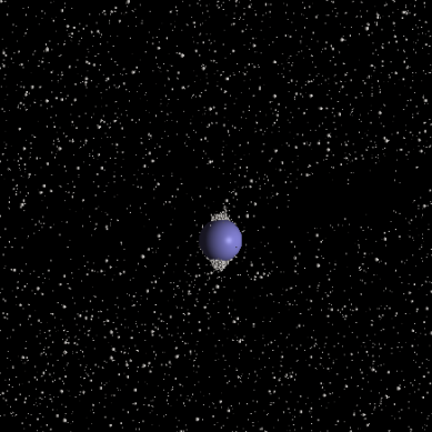
[, ]
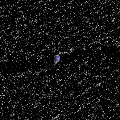 \subbottom[, ]
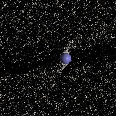
[, ]
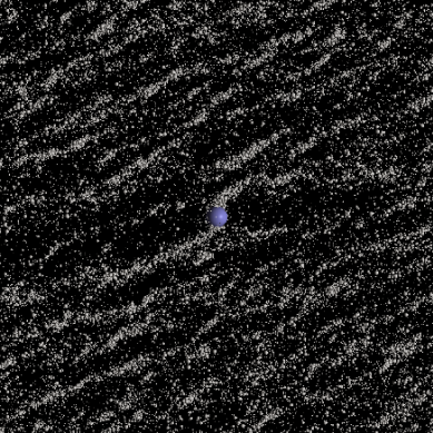 \subbottom[, ]
6 Results
1 Impact bands
The impact band window functions , and are necessary to estimate the damping timescales and the strength of the excitation. To measure those, each particle that enters the box is labelled with its impact parameter. The possible outcomes are plotted in figure 1: (a) being a circulating particle which leaves the box on the opposite side, (b) representing a collision with other ring particles close to the moonlet where the maximum distance from the centre of the moonlet has been taken to be twice the moonlet radius, (c) being a direct collision with the moonlet and finally (d) showing a horseshoe orbit in which the particle leaves the box on the same side that it entered.
The impact band (b) is considered in addition to the impact band (c) because some ring particles will collide with other ring particles that are (temporarily) bound to the moonlet. Thus, these collisions take part in the transfer the energy and momentum to the moonlet. Actually, if the moonlet is simply a rubble pile of ring particles as suggested by Porco et al. (2007), then there might be no solid moonlet core and all collisions are in the impact band (b).
Figures 6 and 7 show the impact bands, normalised to the Hill radius of the moonlet for simulations EQ5025, EQ20025, EQ40050, EQ5050, EQ20050 and EQ40050. For comparison, we also plot sharp cutoffs, at and , as these have been used in same of the scaling laws presented above.
Note that because ring particles are shifted from time to time when the moonlet is too far away from the origin (see section 1). In this process, particles with the same initial impact parameter might become associated with the more than one impact band.
Our results show no sharp discontinuity because of the velocity dispersion in the ring particles which is . The velocity dispersion corresponds to an epicyclic amplitude of or equivalently and (for and , respectively). Note that the Hill radius is approximately equal to the physical radius of the moonlet. This is because the moonlet will always fill its Roche lobe with ring particles (see also Porco et al., 2007).
The impact bands are almost independent of the surface density and depend only on the Hill radii and the mean epicyclic amplitude of the ring particles, or, more precisely, the ratio thereof. Thus we expect the impact bands to have a cutoff width of . A simple approximation of the impact bands may then be given by
| (50) | |||||
| (51) | |||||
| (52) |
These curves are plotted on the right hand side of figures 6 and 7, being qualitatively very similar to the measured impact bands. This approximation ignores the non-spherical shape of the Roche lobe and assumes .
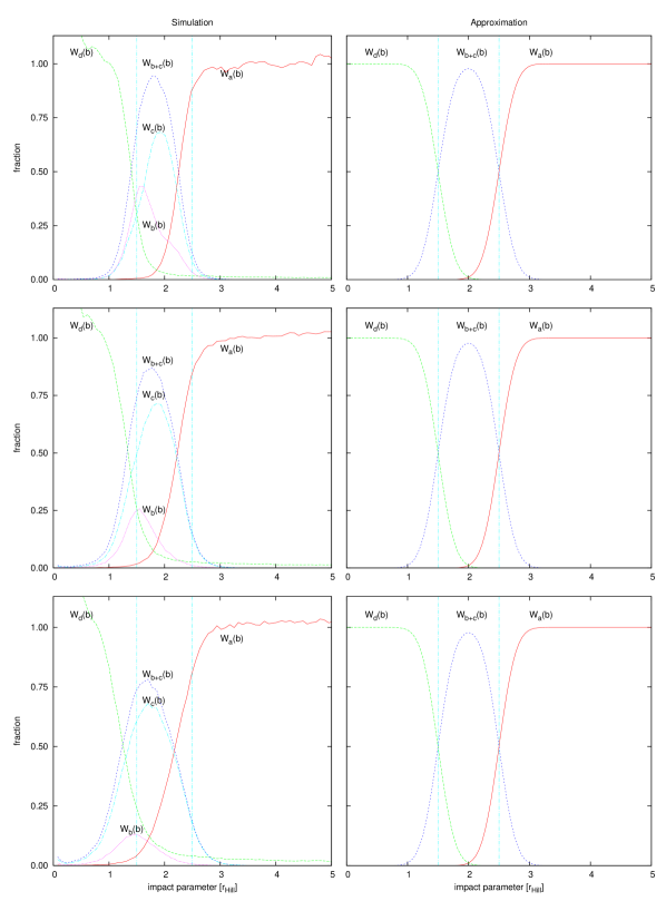
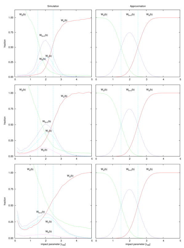
2 Eccentricity damping timescale
To measure the eccentricity damping timescale, we first let the ring particles and the moonlet reach an equilibrium and integrate them for 200 orbits. We then change the velocity of the moonlet and the ring particles within . The new velocity corresponds to an eccentricity of , which is well above the equilibrium value. We then measure the decay timescale by fitting a function of the form
| (53) |
The results are given in table 2. They are in good agreement with the estimated damping timescales from section 1 and 2, showing clearly that the most important damping process, in every simulation considered here, is indeed through collisional damping as predicted by comparing equation 15 with equations 19 and 21.
| Name | Numerical results | Analytic results | |
|---|---|---|---|
| collisions | horseshoe | ||
| EQ5025 | 18.9 | 18.4 | 1712 |
| EQ5050 | 27.6 | 33.8 | 3424 |
| EQ20025 | 9.0 | 3.9 | 428 |
| EQ20050 | 12.9 | 8.5 | 856 |
| EQ40025 | 2.8 | 2.1 | 214 |
| EQ40050 | 5.5 | 4.4 | 428 |
3 Mean moonlet eccentricity
| Name | Numerical results | Analytic results | |||
|---|---|---|---|---|---|
| collisions | circulating particles | circulating clumps | total | ||
| EQ5025 | |||||
| EQ5050 | |||||
| EQ20025 | |||||
| EQ20050 | |||||
| EQ40025 | |||||
| EQ40050 | |||||
| Name | Numerical results | Analytic results | ||||
|---|---|---|---|---|---|---|
| horseshoe | collisions | circulating particles | circulating clumps | total | ||
| EQ5025 | 22.7m | 9.0m | 10.5m | 17.6m | 0.3m | 22.4m |
| EQ5050 | 12.6m | 4.5m | 4.8m | 4.4m | 0.1m | 7.9m |
| EQ20025 | 38.1m | 18.1m | 25.1m | 17.6m | 15.7m | 38.9m |
| EQ20050 | 22.7m | 13.6m | 9.6m | 4.4m | 4.8m | 14.7m |
| EQ40025 | 78.1m | 25.6m | 36.5m | 17.6m | 86.6m | 100.7m |
| EQ40050 | 45.6m | 12.8m | 13.4m | 4.4m | 31.4m | 36.7m |
The time averaged mean eccentricity of the moonlet222Here, we are calculating the mean eccentricity, not the root-mean-square eccentricity. is measured in all simulations after several orbits when the ring particles and the moonlet have reached an equilibrium state. To compare this value with the estimates from section 1 we set equation 32 equal to zero and use the analytic damping timescale listed in table 2. The analytic estimates of the equilibrium eccentricity are calculated for each excitation mechanism separately to disentangle their effects. They are listed in the third, fourth and fifth column in table 4. The sixth column lists the analytic estimate for the mean eccentricity using the sum of all excitation mechanisms.
For all simulations, the estimates are correct within a factor of about 2. For low surface densities, the excitation is dominated by individual particle collisions. For larger surface densities, it is dominated by the excitation due to circulating self gravitating clumps (gravitational wakes). The estimates and their trends are surprisingly accurate, as we have ignored several effects (see below).
4 Random walk in semi-major axis
The random walk of the semi-major axis (or equivalently the centre of epicyclic motion in the shearing sheet) of the moonlet in the numerical simulations are measured and compared to the analytic estimates presented in section 4. We run one simulation per parameter set. To get a statistically meaningful expression for the average random walk after a given time , we average all pairs of and for which . In other words, we assume the system satisfies the Ergodic hypothesis.
then grows like and we can fit a simple square root function (see chapter 4). This allows us to accurately measure the average growth in after orbits by running one simulation for a long time and averaging over time, rather than running many simulations and performing an ensemble average. The measured values are given in the second column of table 4. The values that correspond to the analytic expressions in equations 48, 39, 43 and 45 are listed in columns three, four, five and six, respectively.
For low surface densities, the evolution of the random walk is dominated by collisions and the effect of particles on horseshoe orbits. For large surface densities, the main effect comes from the stochastic gravitational force due to circulating clumps (gravitational wakes).
The change in semi-major axis is relatively small, a few tens of metres after 100 orbits ( days). The change in longitude that corresponds to this is, however, is much larger.
Using the results from chapter 4, namely equations 56 and 60, we can predict the long term evolution of . In the stochastic and laminar case, grows like and , respectively. This behaviour allows us to discriminate between a stochastic and laminar migration by observing over an extended period of time.
Results from individual simulations (i.e. not an ensemble average) are plotted in figure 8. Here, is expressed in terms of the azimuthal offset relative to a Keplerian orbit. One can see that for an individual moonlet, the shift in azimuth can appear to be linear, constant or oscillating on short timescales (see curve for simulation EQ20025). This is partly because of the lower order terms in equation 55, though, on average, the azimuthal offset grows very rapidly, as for (see equation 56).

7 Conclusions
In this chapter, we have discussed the dynamical response of an embedded moonlet in Saturn’s rings to interactions with ring particles both analytically and by the use of realistic three dimensional many particle simulations. Both the moonlet and the ring particle density were taken to be . Moonlets of radius and were considered. Particle sizes ranging between and were adopted.
We estimated the eccentricity damping timescale of the moonlet due to collisions with ring particles and due to the response of ring particles to gravitational perturbations by the moonlet analytically. We found the effects due to the response of particles on horseshoe and circulating orbits are negligible. On the other hand the stochastic impulses applied to the moonlet by circulating particles were found to cause the square of the eccentricity to grow linearly with time as did collisions with particles with non zero velocity dispersion. A balance between excitation and damping processes then leads to an equilibrium moonlet eccentricity.
We also estimated the magnitude of the random walk in the semi-major axis of the moonlet induced by collisions with individual ring particles and the gravitational interaction with particles and gravitational wakes. There is no tendency for the semi-major axis to relax to any particular value, so that there are no damping terms. The deviation of the semi-major axis from its value at time grows on average as for large
From our simulations we find that the evolution of the eccentricity is indeed dominated by collisions with ring particles. For large surface densities (more than ) the effect of gravitational wakes also becomes important, leading to an increase in the mean steady state eccentricity of the moonlet. When the particle velocity dispersion is large compared to we obtain approximate energy equipartition between the moonlet and ring particles as far as epicyclic motion is concerned.
Similarly, the random walk in the semi-major axis was found to be dominated by collisions for low surface densities and by gravitational wakes for large surface densities. In addition we have shown that on average, the difference in longitude of a stochastically forced moonlet grows with time like for large
The radial distance travelled within 100 orbits (50 days at a distance of 130000km) is, depending on the precise parameters, of the order of 10-100m. This translates to a shift in longitude of several hundred kilometres. The shift in is not necessarily monotonic on short timescales (see figure 8). We expect that such a shift should be easily detectable by the Cassini spacecraft. And indeed, Tiscareno et al. (2010) report such an observation, although the data is not publicly available yet, at the time when this thesis was submitted.
There are several effects that have not been included in this study. The analytic discussions in sections 2, 3 and 4 do not model the motion of particles correctly when their trajectories take them very close to the moonlet. Material that is temporarily or permanently bound to the moonlet is ignored. The density of both the ring particles and the moonlet are at the lower end of what is assumed to be reasonable (Lewis & Stewart, 2009), which has the advantage that for our computational setup only a few particles (with a total mass of less than 10% of the moonlet) are bound to the moonlet at any given time.
Chapter 6 Planetesimal formation in a turbulent disc
To explain all nature is too difficult a task for any one man or even for any one age. ’Tis much better to do a little with certainty, & leave the rest for others that come after you, than to explain all things by conjecture without making sure of any thing.
Isaac Newton, unpublished preface to Opticks, 1704
In chapter 4, we discussed the evolution of planets and planetary systems under the effect of stochastic forces resulting from turbulence. The stochastic migration of moonlets in Saturn’s rings was discussed in chapter 5. In this chapter, we look at another system, in which turbulence is important, namely the formation of planetesimals, the building blocks of planets.
The formation mechanism of planetesimals in proto-planetary discs is hotly debated. Currently, the favoured model involves the accumulation of metre-sized objects within a turbulent disc. These high spatial densities then promote the formation of planetesimals, for example via gravitational instability as discussed in more detail in chapter 2. In numerical simulations that model this process, one can at most simulate a few million particles as opposed to the several trillion metre-sized particles expected in a real proto-planetary disc. Therefore, single particles are often used as super-particles to represent a distribution of many smaller particles. It is assumed that small-scale phenomena do not play a role and particle collisions are not modelled. However, the super-particle approximation can only be valid in a collision-less or strongly collisional system. In many recent numerical simulations this is not the case.
Here, a scaled system is studied that does not require the use of super-particles. We compare this new method to the standard super-particle approach. We find that the super-particle approach produces unreliable results that depend on numerical artifacts such as the gravitational softening in both the requirement for gravitational collapse and the resulting clump statistics. Our results show that short-range interactions (collisions) have to be modelled properly.
The outline of this chapter is as follows. In section 1, we review the important timescales in the problem and show that the super-particle approach breaks down in high density regions. In section 2, we discuss both the super-particle and the scaled particle method. The numerical implementation and the initial conditions of the simulations are presented in section 3. Results of numerical simulations using both the super-particle approach and our scaling method are presented in section 4. We conclude with presenting resolution constraints for numerical simulations and discuss the implications for the planetesimal formation process through gravitational instability in section 5.
1 Orders of magnitude
1 Definition of timescales
The aim of this work is to simulate the dynamics of dust (or particles) interacting gravitationally inside a turbulent proto-planetary disc. Each particle is subject to five different physical processes, each operating on a typical timescale:
-
Stopping time
Each particle of size feels the effects of the surrounding gas through a linear drag force. This force can be written as , where is the stopping time of a particle of mass , is the velocity of the gas, and is the velocity of the particle (Weidenschilling, 1977a). The stopping time depends on the degree of coupling to the gas (e.g. Chiang & Youdin, 2009):
(1) where and are the internal density of the particles and the density of the gas, respectively. is the mean free path of gas particles and the sound speed.
-
Physical collision timescale
Dust particles will suffer a physical collision with another dust particle on a timescale of , where is the geometrical cross-section of the particles, is the particle velocity dispersion, and is the number density of particles in a homogeneous medium.
-
Orbital timescale
The timescale associated with the particles orbiting the central object in a local shearing patch is the epicyclic period , where is the angular velocity at the semi-major axis of the shearing box.
There are two limits for the gravitational interactions between dust particles, long and short range. The long-range interaction can be seen as a collective process involving interactions between clouds of particles. On the other hand, the short-range interaction is important for resolving close approaches between pairs of particles, i.e. gravitational scattering. For the sake of clarity, we separate these two processes.
-
Gravitational collapse timescale
On a length scale , where is the average distance between neighbouring dust particles, the long-range interaction of the dust particle distribution can be approximated by a continuous density . The gravitational collapse timescale, which is of the order of the free fall time of the system, can be defined by .
-
Gravitational scattering timescale
Short-range gravitational interactions are interactions between a pair of single particles that can result in a scattering event. As with physical collisions, the timescale for a gravitational interaction depends on the cross-section, . Here, is the gravitational cross-section of the particle. Note that the cross-section is velocity dependent, which makes it qualitatively different from physical (billard ball) collisions between two particles.
Particles might also be affected by excitation from a turbulent background state on a timescale defined by the turbulence itself. Unlike in chapter 4, we here model the excitation in an even more simplified way, in which the turbulence is scale independent and has no timescale associated with it.
2 The real physical system
To identify the dominant physical processes in a proto-planetary disc, one has to quantify and compare the relevant timescales as defined above. In the following discussion and in the numerical simulations, we assume AU, a gas disc thickness of , and a minimum mass solar nebula (MMSN) with surface gas density111Note that there are different values for MMSN in the literature. This value here is a factor 5 smaller than the one used in chapter 4. . One usually assumes a solid to gas ratio of . We, however, assume a solid to gas ratio of unity. This value is justified by numerical simulations (Johansen et al., 2007, 2009) that demonstrate over-densities of the order of can easily occur because of the interaction with a turbulent gas disc, the streaming instability, or vertical settling. Thus, we are only interested in the late stages of the planetesimal formation process. The details of how the initial over-density has been achieved are not relevant for the discussion presented in this chapter. We also note that significantly different models of the solar nebula have been proposed (Desch, 2007). However, all results can easily be scaled to different scenarios.
We simplify the system by assuming that all solid components of the disc are in metre-sized particles. We assume that these boulders have a typical velocity dispersion caused by gas turbulence , where is the local sound speed, in accordance with numerical results (Johansen et al., 2007). Since , the particles tend to sediment toward the mid-plane, forming a finite thickness dust layer due to the non-zero velocity dispersion.
For metre-sized boulders, the physical cross-section is , whereas the gravitational scattering cross-section is showing clearly that gravitational scattering is irrelevant to the dynamics of dust particles embedded in a disc. However, all other timescales are roughly equivalent. Metre-sized boulders are weakly coupled to the gas with a stopping time (Weidenschilling, 1977a). The physical collision timescale is and the long-range gravitational interaction timescales is .
This physical system is expected to become gravitationally unstable, according to the Toomre criterion (Toomre, 1964). The instability occurs when the gravitational collapse timescale is shorter than the transit time due to random particle motions and the orbital timescale. Assuming that the particles can be modelled by an isotropic gas222This is formally not valid in the studied regime, as it is not strongly collisional. with a sound speed , the system becomes unstable when (equation 28). In that case, the most unstable wavelength is given by equation 29. In the following, we compare the physical parameters from this section to their counterpart in numerical simulations. We first summarise the super-particle approach before presenting the scaling method.
2 Methods
Two different kinds of simulation are considered in this chapter:
-
1.
Particles are assumed to be point masses and have no physical size, the gravitational field of the particles being approximated with a smoothing length to avoid numerical divergences (see section 1).
-
2.
Particles have a physical size and, therefore, no gravitational smoothing is required but physical collisions must be included.
We refer to the particles as super-particles and scaled particles, respectively.
1 Super-particle approximation
Let us quickly review the standard approach using super-particles before moving on to studying our favoured method that uses scaled particles.
A super-particle represents many smaller particles. The dynamics of the small particles are not calculated exactly. It is assumed that all particles behave similarly and in a collective manner. To simulate gravitational interactions between super-particles, one has to use a softened potential. Without this, the gravitational scattering cross-section of super-particles becomes too large and super-particles undergo gravitational scattering events, which are unphysical since these events never occur in a real system. Individual particle-particle collisions are not modelled.
There are various examples where this approach is used successfully. For example, smoothed particle hydrodynamics (SPH) uses the super-particle approximation to simulate many gas molecules (Lucy, 1977). These systems are often assumed to be strongly collisional to ensure thermodynamical equilibrium inside each super-particle. One can therefore assign collective properties to clouds of particles such as pressure and temperature. Another example is the evolution of galaxies. When two galaxies collide, individual particles (stars) will usually not undergo gravitational scattering events or physical collisions. In that case, the super-particle approach models a collision-less system in which collective dynamics are the only important physical process. In both cases, the super-particle approximation is a valid approach for simulating the system numerically, but will break down as soon as the system is marginally collisional.
As an example, we consider two clouds of particles undergoing a “collision”. In the strongly collisional case, the clouds will slowly merge and the thermodynamic variables (e.g., temperature) will diffuse between the clouds, the particles inside each cloud following a random walk trajectory due to numerous collisions. On the other hand, in the collision-less regime, the two clouds simply do not see each other because there is no short-range interaction present between the particles. In a marginally collisional regime, some particles will collide with particles of the other cloud, leading to a partial thermalisation of the velocity distribution, but some other particles will not have any collision at all and will follow approximately a straight line. Evidently, the outcome of this event cannot be described using a super-particle approach.
2 Scaling method
The idea of the scaling method is that one should keep all important timescales in a numerical simulation as close to those of the real physical system as possible and model all particle collisions explicitly.
The numerical system consists of particles in a box with length , simulating a patch of the disc at a fixed radius . The particle mass is ( is the box size and one scale height). Thus, the density in the box and the long-range gravitational interactions are unchanged compared to the real system.
The gravitational scattering cross-section of the numerical system is then given by
| (2) |
For the initial surface density and velocity dispersion used in the simulation (see above), one finds
| (3) |
The physical collision cross-section in the simulation is where , is the radius of the particles in the simulation. We derive two constraints from the physical and gravitational collision cross-sections:
-
1.
Same mean free path in simulation and real physical systems
That means , where and are the geometrical cross-section and the number of particles in a region of size in a real disc, respectively. In other words, this condition ensures that the physical collision timescale in the simulation is exactly the same as in the real system.
-
2.
Negligible gravitational scattering
When two particles approach each other, the outcome should be a physical collision, which means that . The gravitational scattering timescale remains long compared to the physical collision timescale.
The first condition places a constraint on the particle size in the simulation. With and a particle radius of as found in a real disc within a box of volume , using the parameters from above one finds that
| (4) |
We note that once this condition is satisfied in the initial conditions it will be automatically satisfied at all times. In simulations, we typically find that the collision timescale is reduced by more than one order of magnitude during the gravitational collapse.
The second condition is then satisfied by changing the number of particles. An interesting result is that if , the second condition is easily satisfied if the first one is satisfied. However, depends strongly on the velocity dispersion. In particular, a velocity dispersion 5 times smaller than the initial value (as found in some simulations) leads to an increase by a factor of 600 in the gravitational scattering cross-section. Therefore, we suggest using a large safety factor () to ensure that the second condition is always satisfied, even for significantly smaller . This condition also allows us to estimate when our approach breaks down, namely when the number of clumps in the system is so low () that gravitational scattering becomes important.
Although it would be helpful as a further simplification, it is not possible to perform the above mentioned simulation in two dimensions. In that case, the filling factor, which is defined to be the ratio of the volume (or area) of all particles to the total volume (or area), is of the order of one for the above parameters. We note that in 2D an increase in particle number (and decrease in particle size as required by equation 4) does not decrease the filling factor if the collisional lifetime remains constant.
3 Numerical simulations
We perform our simulations in a cubic box with shear periodic boundary conditions in the radial () and periodic boundary conditions in the azimuthal () and vertical () directions, as described in appendix 11. In the local approximation, the force per mass on each particle is a sum of the contributions from Hill’s equations (see equations 8-10) and interaction terms. The interaction terms are divided into components related to self gravity (including vertical gravity), physical collisions between particles, or drag and excitation forces:
| (5) |
We solve the resulting equations of motion with a leap frog (kick drift kick) time-stepping scheme. In the following subsections, we describe how each of these terms are calculated and what their physical relevance is.
The box size of was chosen such that there are always several unstable modes in the box, when the system is pushed into the regime of gravitational collapse, as estimated by equation 29.
1 Self gravity
In the -body problem that we consider, we have to solve Newton’s equations of universal gravitation for a large number of particles . Calculating the gravity for each particle from each other particle results in operations. To reduce the number of operations, we use an approximation, namely a Barnes-Hut (BH) tree code (see appendix 11).
We use rings of ghost boxes in the radial and azimuthal direction. The system that we are interested in is only marginally gravitationally stable and due to the finite number of ghost boxes, we introduce a slight asymmetry that will become important after several orbits. In the beginning of our simulations, we integrate for many orbits in order to reach a stable equilibrium. We then push the system into a gravitationally unstable regime (see section 5 for details). During the stable phase, horizontal over-concentrations are to be expected and are indeed observed because of this asymmetry. However, since in a real proto-planetary disc the gravitational instability is considered to appear locally (e.g., inside a vortex or a similar structure), this effect of having a preferred location for gravitational instability is not unphysical and does not affect any conclusions made. We tested this by applying a linear cut-off to the gravitational force at a distance of one box length (A. Toomre, private communication). In this case, there was no preferred location in the box and the simulation evolved in exactly the same way.
2 Physical collisions
Physical collisions between particles are treated by checking whether any two particles are overlapping after each time-step. Using the already existing tree structure from the gravity calculation, one can again reduce the computational costs from to . There is a small probability that we might miss a collision if the time-step is too large. To ensure that our results are converged, we tested that a reduced time-step does not alter the outcome. See appendix 11 for more details on how collisions are resolved.
The particle radius is given by equation 4. In order to keep the collision timescale close to unity, which is numerically the worst case scenario because all timescales are equivalent, we increase the radius by a factor of 4 in all simulations.
3 Drag force
Each particle feels a drag force. The background velocity of the gas is assumed to be a steady Keplerian profile
| (6) |
Although accretion flows are turbulent, we choose to use a simple velocity profile so that the behaviour of self-gravitating particles can be understood in conditions that can be easily controlled.
4 Random excitation
The system of particles described above is dynamically unstable even without self-gravity, as the coefficient of restitution and the stopping time do not depend on the particle velocities. The particles can either settle down in the mid-plane and create a razor-thin disc if the stopping time is too short, or they can expand vertically forever if the stopping time is above some critical value and the excitation mechanism is provided only by collisions. Dust particles in accretion discs are found in the settling regime. However, a complete settling never occurs in accretion discs because the background flow is always turbulent due to the Kelvin-Helmholtz instability (Johansen et al., 2006), the MRI, or other hydrodynamic instabilities (see e.g. Lesur & Papaloizou, 2009) which diffuse particles vertically (Fromang & Papaloizou, 2006). This stirring process of turbulence is not present in the gas velocity field of the simulations presented here (see equation 6). To approximate the turbulent mixing, we add a random excitation (white noise in space and time) to the particles in the simulation. This allows us to have a well defined equilibrium in which the system is stable rather than starting from unstable initial conditions that might influence the final state.
We perturb the velocity components of each particle after each time-step by , where is the current time-step and is a random variable with a normal distribution around and variance . This excitation mechanism heats up the particles and allows us to have a well defined three dimensional equilibrium as shown in section 4. In our simulations, we use a value of and for the simulations without and with collisions, respectively. These values were chosen such that the equilibrium state is approximately equivalent for both types of simulations.
In comparison to chapter 4, here we try to simplify things as far as possible. Thus, the description of stochastic forces used leads to uncorrelated and scale independent noise.
5 Initial conditions
All particles, which have equal mass, smoothing length, and physical size, are placed randomly inside the box in the plane. We note that particles have either a physical size or a smoothing length associated with them, depending on the type of simulation we perform. In the z-direction, the particles are placed in a layer with an initially Gaussian distribution about the mid-plane and a standard deviation of 0.05 H. We allow the system to reach equilibrium by integrating it until ().
We tested various ways of pushing the system into the unstable regime. We here present two different scenario. First, one can switch off the excitation mechanism. The systems starts to cool down and thus becomes unstable. Second, one can shorten the stopping time, which leads to enhanced cooling.
Following one of the above descriptions, the system becomes gravitationally unstable and bound clumps form within a few orbits. We did not see any qualitative differences as long as we started from a well defined equilibrium state. This shows that, even though we simplified the treatment of turbulent stirring and gas drag, the results are generic.
4 Results
1 Super particles
We first present simulations without physical collisions (super-particles) which rely on the smoothing length to avoid any divergences. Although we use a tree code and a smoothed potential for the force calculation is assumed, the results are equivalent to an FFT-based method (Fast Fourier Transform) where the grid length acts as an effective smoothing length. In general, to check the numerical resolution, the particle number is increased and the smoothing length is reduced independently. A simulation is resolved when the result is independent of both and . This turns out to be impossible in the present situation. The main reason is that the smallest scale in a gravitational collapse will ultimately depend on the smoothing length. By varying both parameters at the same time, an empirical scaling of works fairly well if is large enough. The square root in this scaling comes from the fact that we are basically treating a two dimensional system. However, this procedure is not justified and is unphysical. The smoothing length was introduced to avoid divergent terms and not to model any small-scale physical process. Therefore, it should not have any impact on the physical outcome of the simulation. Incidentally, the existence of this dependency indicates that short-range interactions are important for the result of these simulations and should be modelled with care.
In figure 1, we plot the velocity dispersion as a function of time. The simulations begin from the stable equilibrium described in section 2. After , we switch off the excitation mechanism. The system continues to cool and it becomes gravitationally unstable within one orbit, as estimated by equation 28. Once clumping occurs, the velocity dispersion begins to rise again. All simulations use the particle radius given by equation 4 as a smoothing length except the ones labelled LS, which use a value ten times larger. The larger softening length is approximately -th of the box length and illustrates the kind of evolution expected from an FFT method using a grid. This is the resolution used in other studies, such as Johansen et al. (2007).
The velocity dispersion evolution is also plotted in figure 2 for those simulations, in which the damping timescale has been decreased while keeping the excitation unchanged. The results are qualitatively very similar to those presented in figure 1.
Snapshots of the particle distribution of two simulations are shown in figure 3. Both simulations use 160 000 particles and all parameters, except the smoothing length, are the same. The top row is the simulation with a smoothing length given by equation 4, whereas the bottom row uses a smoothing length that is ten times larger. The simulations correspond to the blue (medium dashed) and red (solid) curve in figure 1. We show the snapshots to illustrate the importance of the smoothing length in simulations without physical collisions. One can see that the simulations differ already before clumps form. Stripy structures appear on a scale given by equation 29. As soon as we enter the unstable regime at (i.e., the velocity dispersion begins to rise, see also figure 1) the simulations evolve very differently. The simulation on the top row of figure 3 forms many clumps at an early time, whereas the bottom row simulation forms only a few, more massive clumps at later times.
This can be confirmed by looking at spectra of the same two simulations as shown in figure 5. These spectra were generated by mapping the particles onto a grid in the plane and computing the fast Fourier transform of the mapping in the direction. The resulting spectra were finally averaged in the direction (see Tanga et al., 2004, for a complete description of the procedure). As suggested by the snapshots, the nonlinear dynamics of the gravitational instability strongly depends on the smoothing length used. In particular, one observes that smaller scales are amplified more slowly for larger smoothing lengths. The resulting spectra at also differ significantly. With a small enough smoothing length, the spectrum looks almost flat, whereas a large smoothing length introduces a cutoff at . We also note that the smoothing length in the latter case is of the order of the grid size (). The cutoff observed clearly demonstrates that the smoothing length modifies the dynamics on scales up to 10 times larger than the smoothing length itself.
[Super-particles. The simulation labelled LS has a ten times larger smoothing length. The curves do not overlap because the simulations have not converged. ]
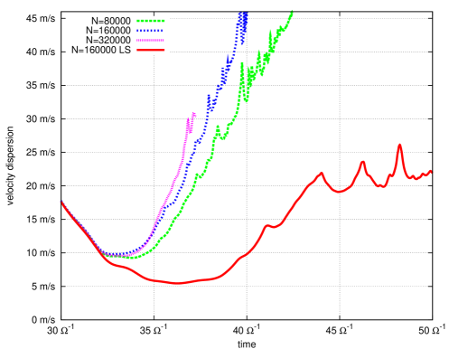 \subbottom[Scaled-particles. All curves overlap at early times because the simulations are converged (see text). ]
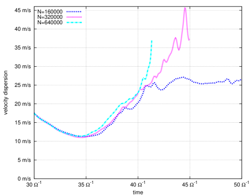
[Super-particles. The simulation labelled LS has a ten times larger smoothing length. The curves do not overlap because the simulations have not converged. ]
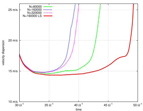 \subbottom[Scaled-particles. All curves overlap because the simulations are converged. ]
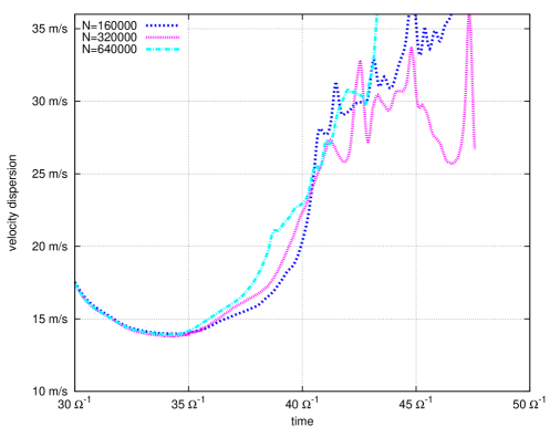
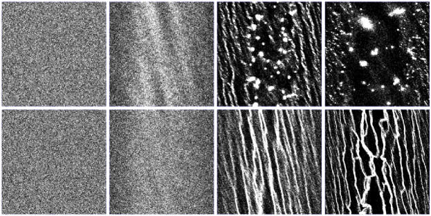

2 Scaled particles
[Super-particles: Spectrum with 160 000 particles and two different smoothing lengths that differ by a factor 10 at times (red, solid curve), (green, long dashed curve), and (blue, short dashed curved). The spectra at similar times are not on top of each other because the simulations have not converged.]
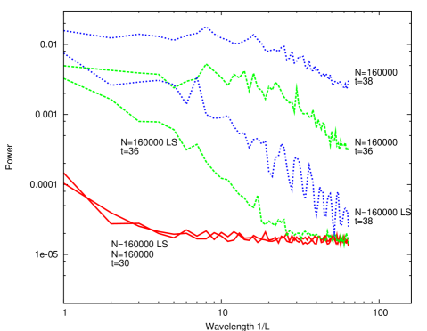 \subbottom[Scaled particles: Spectrum with 160 000, 320 000, and 640 000 particles (colours are equivalent to figure 5). At each time, the spectra are converged, i.e., the spectra are on top of each other and independent of the particle number, besides the noise level on very small scales. At late times (, blue curve), one begins to see more structure on small scales in simulations with larger number of particles (see text). ]
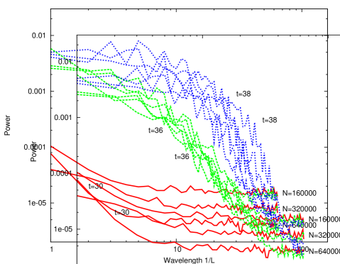
The velocity dispersion evolution of simulations with particles including physical collisions is presented in figure 1 and figure 2. In these runs, no gravitational smoothing length is needed. Again, the simulations start from a stable equilibrium and after , we change the same parameters as in the non-collisional case to push the system into the gravitationally unstable regime. In figure 1 we increase the damping timescale, whereas we switch off the excitation in figure 2. Snapshots of the particle distribution for three runs are plotted in figure 4. The middle and bottom rows of snapshots correspond to the purple (medium dashed) and dark blue (long dashed) lines of figure 1.
One can see in figures 1, 2 as well as figure 4 that the intermediate and high resolution runs produce very similar results. We call those simulations converged, as a change in particle number does not change the outcome. An additional, lower resolution run () has not converged because the filling factor is too large in dense regions, preventing clumps from being gravitationally bound. The problem does not occur in the non-collisional cases because particles are allowed to overlap. Since the filling factor scales with particle number as , this issue is resolved for runs with more than a few hundred thousand particles. We note that the velocity dispersion might differ at later stages for the converged runs because the final clump radius is still determined by the physical particle radius and therefore by the particle number. This can be seen in particular in figure 1 where the velocity dispersion of the run reaches an equilibrium value before the runs with larger particle number. Note however, that up to that point, the results are converged.
We show the density distribution spectrum in figure 5 as a function of the number of particles. The resulting spectra do not depend on the number of particles in the system, as expected. In comparison with figure 5, the simulations with collisions are converged since the dynamic has not controlled by the numerical parameter , which is the only free parameter in the system.
At very late times (), the spectra begin to show a systematic trend towards more structure on smaller scales for runs with larger . This is due to the filling factor, already mentioned above. When the size of a clump in the simulation is only determined by the size of the individual scaled particles that it consists of, our approach breaks down. One can also see these clumps forming by looking at the velocity dispersion in figure 1. The particles inside a clump begin to dominate the velocity dispersion over the background after . A clear indication of this is the spiky structure with a typical correlation time of corresponding to different clumps interacting and merging with each other. One way around this issue, which will be considered in future work, is to allow particles to merge (Michikoshi et al., 2009). Using this specific accretion model, the mass of the clump can then be used as an upper limit of the clump mass. Eventually, one should also worry about possible effects leading to the destruction of an already formed clump.
5 Discussion and implications
In this chapter, we have shown that convergence in -body simulations of planetesimal formation via gravitational instability can be achieved when taking into account all relevant physical processes. It is absolutely vital to simulate gravity, damping, excitation, and physical collisions simultaneously, as the related timescales are of the same order and therefore all effects are strongly coupled.
A set of simulations is defined to be converged when the results do not depend on the particle number or any other artificial numerical parameter such as a smoothing length. As a test case, a box with shear periodic boundary conditions was used, containing hundreds of thousands of self-gravitating (super-)particles in a stratified equilibrium state. The particles were then pushed into a self gravitating regime that eventually led to gravitational collapse. Simulations with and without physical collisions were studied for a range of particle numbers to test convergence.
In cases without physical collisions, convergence can not be achieved. However, it was possible to change multiple free simulation parameters at the same time, namely the particle number and the smoothing length , such that in special cases the results did not depend on the particle number. We note however that there is a free parameter in the simulation (i.e., the smoothing length) that effects the outcome and makes it impossible to find the real physical solution.
In the proto-planetary disc, physical collisions dominate over gravitational scattering. In the case of planetesimal formation, the system is marginally collisional. Physical collisions will partially randomise the particle distribution, whereas a smoothing length does not because the softening length is very large compared to the gravitational cross-section. Even if the gravitational particle-particle scattering becomes important, it can be seen from equation 2 that the velocity dependence of the cross-section differs fundamentally from the velocity independent cross-section . We therefore argue that the super-particle approach should not be used when collisions become important.
With collisions, the simulation outcome is both quantitatively and qualitatively very different from simulations with no physical collisions. The initial size of the clumps is larger and the number of clumps is smaller. As there is no smoothing length, there is effectively one fewer free parameter. Changing the particle number while keeping the collision time constant does not change the outcome. We therefore call these simulations converged.
Additional tests including inelastic collisions with a normal coefficient of restitution of have been performed to confirm that the results do not depend on the way physical collisions are modelled. As expected, the qualitative outcome in terms of number of clumps and clump size is different because the physical properties of the system have been changed. However, once individual collisions are resolved the results converge in exactly the same manner as in those simulations presented above which have a coefficient of restitution of .
This chapter focused on the numerical requirements to study gravitational instability and the formation of planetesimals in proto-planetary discs. The initial conditions were chosen such that the equilibrium is a well defined starting point for the convergence study. The collision, damping, collapse and orbital timescales are all of the same order, which is effectively the worst case scenario. To provide any constraints on planetesimal formation itself, one would have to properly simulate the turbulent background gas dynamics which is a far bigger task.
However, we were able to determine the numerical resolution needed to resolve dust particles in a proto-planetary disc. Assuming that one wishes to simulate dust particles realistically, including collisions, and that the particles are uniformly distributed in a box of base and height , the size of each particle is determined by the collision rate in the real disc (see equation 4)
| (7) |
where and are the size and number of particles in the volume of the real disc. The number of particles in the simulation has to be large enough to ensure that the filling factor is low until clumps form. The requirement that the filling factor is less than unity at is given by
| (8) |
where is a safety factor. Although would be enough to resolve collisions initially, it is insufficient to simulate the collapse phase. During the collapse, the filling factor rises rapidly. Assuming that one wishes to resolve collisions correctly when the particles have contracted by one order of magnitude, one has to include a safety factor of . If the collapse occurs mainly in two dimensions, as in the simulations presented here, a factor of is sufficient. Furthermore, one has to ensure that the box contains at least a few unstable modes (see equation 29). All this together places tight numerical constraints on numerical simulations of planetesimal formation via gravitational instability.
In the future, the discussion should be expanded to include more physics, namely a proper treatment and feedback of the background gas turbulence. This will allow us to further clarify the behaviour of planetesimals in the early stages of planet formation and eventually test the different formation scenarios.
Chapter 7 Summary
If I have seen further it is only by standing on the shoulders of giants.
Issac Newton, in a letter to Robert Hooke, 1676
Several hundred extra-solar planets have been discovered in recent years. This led to a revival of planet formation theory. The remarkable differences of extra-solar planetary systems and our own solar system keep challenging long standing theories.
In this thesis, four main results are presented and summarised below. They can be categorised into two groups. One group is concerned with the formation of resonant multi-planetary systems. The other group discusses the effects of stochastic forcing on orbiting bodies such as planets, moonlets and dust.
1 Main results
1 Most resonant planetary systems are stable
In chapter 4, we develop a consistent framework for the treatment of stochastic forces in celestial mechanics. The growth rates of all orbital parameters are given as a function of the diffusion coefficient in the most generic way. Furthermore, several important correction factors which take into account a finite correlation time are included. Previous studies have overestimated the diffusion efficiency by more than an order of magnitude by ignoring these effects.
We apply this framework to a single, stochastically forced planet and to two planets that are in resonance. The results show that most planetary systems are stable against the random forces originating from MRI turbulence. This remains true even when we take into account the considerable uncertainties in the amplitude of those forces.
We find that resonant planetary systems have two different modes, which respond differently to stochastic forcing. Thus, systems that did undergo a random walk phase during their evolution should show evidence of that. One system, in which this might have been observed, is HD128311. We present several successful formation scenarios of this system which can reproduce the observed libration pattern. This cannot be obtained using laminar convergent migration alone.
The framework has a wide range of applications including Saturn’s rings (see chapter 5) and promises to have a large impact on future studies involving stochastic forces of any type.
2 First prediction of orbital parameters of exo-planets
The planetary system HD45364 is in a 3:2 resonance. The system cannot be formed by convergent migration with moderate migration rates. The final configuration is always a 2:1 resonance, not the observed 3:2 resonance.
In chapter 3, we present a successful formation scenario that involves a short phase of rapid inwards type III migration. A disc with a mass about five times that of the minimum mass solar nebula is sufficient to drive type III migration. Furthermore, a large disc scale height is favourable for the long term sustainability of the resonance. These results imply that planets form in discs which are more massive than previously thought.
Finally, the outcome of hydrodynamical simulations are directly compared to the measured radial velocity curve. We find a new orbital solution, based on the simulation results, that has a lower value than the previously reported best fit. The eccentricities of both planets are considerably smaller. The results are generic, as in all simulations we perform and that form a 3:2 commensurability, the orbital parameters are almost identical. This difference is the first prediction of the precise orbital configuration of an extra-solar planetary system. It can be verified with new radial velocity measurements within the next few years.
This study opens a new window to quantitative and predictive studies of the dynamics of planetary systems beyond our own solar system.
3 Moonlets in Saturn’s rings migrate stochastically
An analytic estimate of both the random walk in semi-major axis and the mean equilibrium eccentricity of a small moonlet which is embedded in Saturn’s rings is presented in chapter 5. We show that the most important effects that determine the dynamical evolution of the moonlet are collisions with ring particles. If the surface density of the rings is sufficiently large that gravitational wakes can form, then those exert an additional force on the moonlet which becomes dominant eventually. No matter how the moonlet is excited, it will migrate stochastically, with its semi-major axis changing on average like for large .
We perform realistic three dimensional collisional N-body simulation of up to half a million self-gravitating ring particles and confirm the analytic estimates within a factor of two. New, pseudo shear periodic, boundary conditions are used which allow us to use a much smaller shearing patch than previous authors and we therefore get a large performance boost.
The random walk in semi-major axis leads to changes in the longitude that are observable with the Cassini spacecraft. If confirmed, this can be used to calculate an upper limit on the age of the propellers and eventually the ring system itself.
4 Physical collisions are vital in numerical simulations of planetesimal formation
In chapter 6, we revisit the numerical requirements in simulations of planetesimal formation via gravitational instability. We find that the inclusion of collisions is indispensable to obtain a consistent model. If collisions are not included, gravitational scattering is the only small scale process present. It will therefore become very important as soon as clumping occurs. Naively, one might think that gravitational close encounters could be treated as if these were physical collisions. However, properties such as the cross section are different compared to physical collisions and gravitational scattering can therefore not resemble the real system.
The results show that earlier studies should not be trusted beyond the initial clumping phase. Estimates on the minimum number of particles required for convergent results are given.
Future studies on planetesimal formation will have to address this issue and the method presented here shows a clear way on how to do that. This will lead to self-consistent results in future simulations.
2 Future work
1 Multi-planetary systems
The results on multi-planetary systems in this thesis, as successful as they might be, have been restricted to only two systems. However, over a third of the discovered planets are confirmed to be in multi-planetary systems.
Having developed all necessary tools in chapters 3 and 4, it is now an easy task to study many systems in a similar fashion. In the following years, I will select up to 15 multi-planetary systems and study their evolution with both N-body as well as two and three dimensional hydrodynamic simulations. This will be the first survey of realistic formation scenarios among multi-planetary systems. The results will be more precise and not as degenerate as population synthesis models of single planets.
New observations suggest that a substantial fraction of hot Jupiters might be in retrograde orbits (Triaud et al. 2010, in preparation). There are various ways to form these systems, such as Kozai Migration or planet-planet scattering (Fabrycky & Tremaine, 2007; Nagasawa et al., 2008). So far, these methods have not been studied in combination with the traditional ideas of planet-disc interaction. I will use Prometheus to study highly inclined systems in the presence of gas discs.
I also want to continue studying the effects of MRI turbulence on planetary systems. The strength of stochastic forces coming from turbulence is not well constrained yet. For that reason a large interval of possible values of the diffusion coefficient had to be studied in chapter 4. Using the MHD module of Prometheus or a different MHD code such as Athena, I will explore the parameter space in a systematic way with global non-ideal MHD simulations. The measurements of statistical properties of MRI turbulence will improve the predictive capability of our analytic random walk model significantly.
One needs at least 16 (maybe 32 or even 64) grid cells per scale-height to simulate the turbulent proto-stellar disc accurately. Assuming one wants to simulate a radial domain ranging from 1 to 4 AU and 6 scale-heights in the vertical direction, one needs a 96x480x502 grid. This is a challenging task. During my PhD, I have gained knowledge on how to speed up calculations using CPU specific hardware features. If the performance of the code becomes an issue and it turns out that higher resolution is required to simulate the relevant scales in the system, I can implement these changes to speed up the simulations.
With these new results, I am going to show that a broad selection of systems can be formed in a turbulent disc and prove if there is statistically significant observational evidence of turbulence in the exo-planet distribution or not.
2 Saturn’s rings
The work presented in chapter 5 was limited to a rather small subset of the parameter space. I plan to extend this study to a wider range of parameters, especially to higher internal densities and a broader size distribution to reduce granularity. As soon as observational data has been published, I will investigate the constraints arising from the measured random walk of moonlets. If the random walk is indeed as strong as predicted, it is possible to obtain an upper limit on the age of the ring system.
Direct simulations of planetary rings are constrained to a local model. Although this is a valid approximation in most circumstances, it has also certain drawbacks. For example, simulations presented in chapter 5 capture the random walk in semi-major axis but do not capture the net migration over long timescales (Crida et al., 2010).
I plan to extend direct simulations of Saturn’s rings to a global model. Periodic boundary conditions in the azimuthal and pseudo shear periodic boundary conditions in the radial direction, in a similar manner to those presented in chapter 5 and appendix 11, can be used to extend the shearing box to a wedge that extends radially over several tens or hundres of kilometres. We can get rid of Hill’s equations and solve the planet’s gravitational force directly.
Numerically, this is a challenging task, as the number of particles will be very large. Therefore, the particles have to be distributed across processors. As outlined in some detail in appendix 11, MPI is not ideally suited for parallelising tree structures. In this case, however, the fact that one dimension is much larger than the others comes in handy because boxes far away do not have to communicate directly with each other so that their interaction can be pre-calculated.
3 Planetesimal formation
The results on planetesimal formation presented in this thesis are preliminary, showing that it is indeed possible to simulate the gravitational collapse of a self-gravitating planetesimal population. To do this self consistently, one has to include collisions and gas dynamics. The former part has been completed in chapter 6. The latter part has been done by other authors (e.g. Johansen et al., 2007). A combination of both is the logical next step.
Many groups are currently working on planetesimal formation in a turbulent disc. I plan to focus on the differences between global simulations and the local shearing box approximation which has been used by most authors. This is essential to understand the importance of effects such as the streaming instability which rely on a large over-density in the solid to gas ratio. In a local simulation with periodic boundary conditions, this ratio is set by the initial conditions and cannot change. However, in a real proto-stellar disc, as well as in global models, the ratio is controlled by large scale structures in the disc such as pressure and temperature gradients.
To gain a better understanding of these global effects, I will couple the new method that treats particles correctly to a global MHD simulation. The method to solve the non-ideal MHD equations will be the same as for the study of multi-planetary systems. To simulate the self-gravity and collisions in the dust layer, I will re-use the GravTree code, presented in appendix 11, which is ideally suited for this project and already fully developed and tested.
4 Numerical codes
The primary codes that have been written for this thesis, Prometheus and GravTree, will be made publicly available. Both codes will be hosted on github at http://github.com/hannorein/ under the open source license GPL. They are easily portable to different architectures as they are written in C and C++, respectively, using only standard libraries such as OpenGL, OpenMP and libpng. Compilation is controlled by the GNU autotool suite.
Providing the source code is, in my opinion, a necessity as numerical codes are part of the initial conditions. All results should be easily reproducible. Firstly, this helps to make progress in the subject, and secondly, it also increases the chance to find bugs in the code. It is therefore a win-win situation.
Chapter 8 Orbital elements
In this appendix, the orbital elements of an elliptical orbit are defined. It is a solution to the two body problem, the simplest non-trivial problem in celestial mechanics.
We consider a test particle on an orbit around a central object with mass at the origin. The specific force on the particle is given by where is the position of the particle. Thus, the equation of motion is simply
| (1) |
Taking the vector product of the above equation with evaluates to zero on the right hand side and gives after integrating
| (2) |
where is a constant of motion. The absolute value of is the specific angular momentum. The position and velocity vectors are in the same plane and allowing us to restrict ourselves to the two dimensional case. By switching to polar coordinates and , we can rewrite equation 2, giving . We also rewrite equation 1, giving
| (3) |
The solution to equation 3 can then be written as
| (4) |
where is the eccentricity, is the longitude of pericentre and the semilatus rectum which can be written as . We restrict the further discussion to an elliptic orbit for which . In that case , where is the semi major axis. We define the true anomaly as . We can further more define an average angular velocity, , called the mean motion, where is the orbital period, given by
| (5) |
For a circular orbit, the mean motion is simply , where . Now that we have a mean angular velocity, we can also define a mean angle (the mean longitude), measured from the pericentre of the planet, via
| (6) |
Here, is the time of pericentre passage. grows linearly in time.
Finally, we would like to get an equation for and . The time dependence of equation 4 is hidden in . It turns out that an explicit form does in general not exist and the solution can only be calculated iteratively. We can see this by introducing another angle, the eccentric anomaly (see figure 1). It can be shown (Murray & Dermott, 2000) that a relation between the mean longitude and the eccentric anomaly exists such that
| (7) |
This equation is transcendental but can be solved iteratively, for example with a Newton-Raphson method.
Most of the quantities defined above are plotted in figure 1 for illustrative purposes.
Chapter 9 Dissipative forces
Additional terms can be added to the equations of motion in N-body simulations to describe eccentricity and semi-major axis damping. These forces could result from various sources, including a gaseous disc, a planetesimal disc or tides. The derivation follows Lee & Peale (2001) and some expressions are taken from Murray & Dermott (2000).
We have two additional, non-conservative terms in the equations for both the velocity and acceleration. In a Cartesian coordinate system, these are
| (1) | |||||
| (2) |
The expressions are analogue for the and coordinates. In order to differentiate with respect to and , we have to write the cartesian coordinates in terms of orbital elements. The positions can be expressed as
| (3) | |||||
which simply follow from the definition of the orbital parameters (see appendix 8). By differentiating once, we get expressions for the velocities
We also need expressions for the radius , the time derivative of the radius , and in terms of , , and :
| (5) | |||||
| (6) | |||||
| (7) |
To complete the list of equations, we compute several other derivatives needed to calculate the partial derivatives in equation 1 and 2
| (8) | |||||
Putting everything together, we arrive at the following expressions
| (9) | |||||
| (10) | |||||
| (11) |
The additional terms for each of , , are distinct for variations in :
| (14) |
The final equations 9-14 are then used to calculate the dissipative forces and included in the N-body code (see section 2). Note that the orbital elements have to be calculated every sub-timestep. Depending on the integrator and the required number of force evaluations, this can be numerically expensive.
Chapter 10 Response calculation of particles on horseshoe orbits
In this appendix, we calculate the amplitude of epicyclic motion that is induced by an eccentric moonlet in a small particle on a horseshoe orbit.
Appendix 10.A Interaction potential
Due to some finite eccentricity, the moonlet undergoes a small oscillation about the origin in the local Hill Cartesian coordinate system (see section 1). Its Cartesian coordinates then become , with these being considered small in magnitude. The components of the equation of motion for a ring particle with Cartesian coordinates are
| (1) | |||||
| (2) |
where the interaction gravitational potential due to the moonlet is
| (3) |
with the cylindrical coordinates of the particle and moonlet being and respectively. This may be expanded correct to first order in in the form
| (4) |
The moonlet undergoes small amplitude epicyclic oscillations such that where is its small eccentricity and is an arbitrary phase. Then may be written as
| (5) |
where
| (6) |
gives the part of the lowest order interaction potential associated with the eccentricity of the moonlet.
We here view the interaction of a ring particle with the moonlet as involving two components. The first, due to the first term on the right hand side of equation 4 operates when and results in standard horseshoe orbits for ring particles induced by a moonlet in circular orbit. The second term, equation 6, perturbs this motion when is small. We now consider the response of a ring particle undergoing horseshoe motion to this perturbation. In doing so we make the approximation that the variation of the leading order potential equation 4 due to the induced ring particle perturbations may be neglected. This is justified by the fact that the response induces epicyclic oscillations of the particle which are governed by the dominant central potential.
Appendix 10.B Response calculation
Setting where is the small response displacement induced by equation 6 and linearising equations 2, we obtain the following equations for the components of
| (7) | |||||
| (8) |
From these we find a single equation for in the form
| (9) |
When performing the time integral on the right hand side of the above, as we are concerned with a potentially resonant epicyclic response, we retain only the oscillating part.
The solution to equation 9 which is such that vanishes in the distant past when the particle is far from the moonlet may be written as
| (10) |
where
| (11) |
After the particle has had its closest approach to the moonlet and moves to a large distance from it it will have an epicyclic oscillation with amplitude and phase determined by
| (12) |
In evaluating the above we note that, although vanishes when the particle is distant from the moonlet at large it also oscillates with the epicyclic angular frequency which results in a definite non zero contribution. This is the action of the co-orbital resonance. It is amplified by the fact that the encounter of the particle with the moonlet in general occurs on a horseshoe libration time scale which is much longer than We now consider this unperturbed motion of the ring particles.
Appendix 10.C Unperturbed horseshoe motion
The equations governing the unperturbed horseshoe motion are equations 2 with
| (13) |
We assume that this motion is such that varies on a time scale much longer than so that we may approximate the first of these equations as Consistent with this we also neglect in comparison to in equation 13. From the second equation we than find that
| (14) |
which has a first integral that may be written
| (15) |
where as before is the impact parameter, or the constant value of at large distances from the moonlet. The value of for which the horseshoe turns is then given by At this point we comment that we are free to choose the origin of time such that it coincides with the closest approach at which Then in the approximation we have adopted, the horseshoe motion is such that is a symmetric function of
Appendix 10.D Evaluation of the induced epicyclic amplitude
Using equations 6, 9 and 15 we may evaluate the epicyclic amplitudes from equation 12. In particular we find
| (16) |
When evaluating equation 12, consistent with our assumption that the epicyclic oscillations are fast, we average over an orbital period assuming that other quantities in the integrands are fixed, and use equation 15 to express the integrals with respect to as integrals with respect to We then find and where
| (17) |
with From this we may write
| (18) |
where is the final epicyclic motion of the ring particle and the dimensionless integral is given by
| (19) |
We remark that the dimensionless quantity with being the Hill radius of the moonlet. It is related to the impact parameter by Thus for an impact parameter amounting to a few Hill radii, in a very approximate sense, is of order unity, is of order and the induced eccentricity is of order .
Appendix 10.E Numerical verification
We verify the analytic calculation with the numerical code GravTree (see appendix 11). A moonlet with Hill radius is setup on an eccentric orbit with and . A ring particle is placed on an initially circular orbit far away from the moonlet with different impact parameters that all lead to horseshoe orbits.
The amplitude of epicyclic motion of the ring particle, , is plotted in figure 1 for four test cases with , , and . We also plot the analytic estimates of the final epicyclic motion given by equation 18 as straight lines. The agreement is very good, showing some differences at large . Note that an impact parameter greater than leads to impacts so that the departure from the analytic estimate does not influence the circularisation time calculated in chapter 5 significantly.

Chapter 11 N-body simulations with GravTree
This appendix describes the GravTree code that has been written to solve many body systems. The particles might interact gravitationally and through physical collisions. Modules incorporating gas drag and stochastic forces have also been implemented.
First, the relevant equations of motions are presented, followed by a description of the special symplectic integrator used for these. Second, the Barnes Hut tree code is explained. Finally, tests and optimisation strategies that have been implemented are discussed.
Appendix 11.A Hill’s equations
In many situations it is impossible to simulate an entire accretion disc or planetary ring. For example, in the case of a proto-planetary disc there are about one trillion () metre-sized particles. Numerically, we can only simulate a few million, at most.
Fortunately, it is usually sufficient to simulate a small patch of the disc that includes most of the physics. In such a patch (also known as a shearing sheet) the shear is linearised and geometric effects are ignored. This leads to a well defined set of equations with shear periodic boundary conditions in the radial and azimuthal directions (Wisdom & Tremaine, 1988).
Let us start from the equations of motion of a test particle around a single star at the origin with mass such that the gravitational force can be described by
| (1) |
where is the distance from the star. We now move to a non-inertial frame, rotating with angular frequency . The time derivative of a vector quantity in the new frame is given by
| (2) |
where subscripts i and r denote the inertial and rotating frames, respectively. The acceleration in the rotating frame is thus given by
| (3) |
where is the velocity and is the position vector in the rotating frame. Adopting a coordinate system in the rotating frame where corresponds to the radial direction, to the azimuthal direction and to the rotation axis, setting the origin at a distance away from the star, we can simplify the above equation to get
| (4) | |||||
| (5) |
Linearising equation 1 around gives
| (6) | |||||
| (7) |
where we have assumed a Keplerian rotation, . Thus, the linearised equations of motion for an unperturbed particle orbiting in the rotating frame are
| (8) | |||||
| (9) |
where we have dropped the subscript r. We can also linearise the gravity in the vertical direction to get
| (10) |
This set of local approximations is known as Hill’s equations. We solve these with a symplectic leap frog, kick drift kick, time-stepping scheme which is discussed in more detail in the next section.
Appendix 11.B Symplectic integrator
Symplectic integrators in celestial mechanics have several attractive features, such as conservation of energy up to machine precision. We would therefore like to use such an integrator for solving Hill’s equations numerically. A widely used standard symplectic integrator is leap-frog which can be described by a kick, followed by a drift and another kick sub-time-step (KDK). A possible C implementation of one full time-step with length dt is
void kdk(double* x, double* v, double* a, double dt){
// Kick
v[0] += 0.5 * dt * a[0];
v[1] += 0.5 * dt * a[1];
v[2] += 0.5 * dt * a[2];
// Drift
x[0] += dt * v[0];
x[1] += dt * v[1];
x[2] += dt * v[2];
// Kick
update_force(x,v,a);
v[0] += 0.5 * dt * a[0];
v[1] += 0.5 * dt * a[1];
v[2] += 0.5 * dt * a[2];
}
Here, x, v and a are pointers to the position, velocity and acceleration vectors, respectively. This integrator is symplectic if the forces calculated in update_force(x,v,a) do not depend on the velocities. However, Hill’s equations do depend on the velocities (see equations 8 and 9). Note that the component (equation 10) does not depend on the velocities and thus can be integrated with a standard method. Quinn et al. (2010) describe a new symplectic integrator for Hill’s equations. The changes to the KDK algorithm are minimal and only one additional value per particle has to be saved. A modified version of the above code is
void kdk_quinn(double* x, double* v, double* a, double* Py, double dt){
// Kick
v[0] += -0.5*dt * (OMEGA*OMEGA * r[0] - a[0]);
Py = v[1] + 2.0*OMEGA * r[0] + 0.5*dt * a[1];
v[0] += dt * OMEGA * Py;
v[1] = Py - OMEGA * r[0] - OMEGA * (r[0] + dt * v[0]);
v[2] += 0.5*dt * a[2];
// Drift
x[0] += dt * v[0];
x[1] += dt * v[1];
x[2] += dt * v[2];
// Kick
update_force(x,a);
v[0] += dt * OMEGA * Py;
v[0] += -0.5*dt * (OMEGA*OMEGA * r[0] - a[0]);
v[1] = Py - 2.0*OMEGA * r[0] + 0.5*dt * a[1];
v[2] += 0.5*dt * a[2];
}
Here, OMEGA is the orbital frequency and Py is initialised to v[1] + 2.0*OMEGA * r[0]. Py is a conserved quantity for an unperturbed orbit. Note that the drift step is unmodified. This allows for an unchanged collision detection algorithm, usually performed during the drift sub-time-step. The function update_force() does not include the terms due to Hill’s equation anymore, only additional forces (e.g. gravity from other particles, gas drag, …).
The symplectic integrator has proven to be very useful for integrations of moonlets in Saturn’s rings, where the eccentricity is generally very small and the system is integrated for hundreds of orbits.
Appendix 11.C Gravity calculation
In the -body problem that we are considering here, we have to solve Newton’s equations of universal gravitation for a large number of particles . The gravitational force on the -th particle is given by
| (11) |
where is the smoothing length used to avoid divergencies in numerical simulations. In simulations where particles have a finite size and physical collisions are included we can safely set . The unit vector in the direction of the gravitational force between the -th and -th particle is . Calculating the gravity for each particle from each other particle results in operations. To reduce the number of operations, one can use different approximations to equation 11. Here, we use a Barnes-Hut (BH) tree code (Barnes & Hut, 1986). The BH tree reduces the number of calculations to .
A tree code in three dimensions works by sub-dividing the original box into eight smaller cells with half the length of the original box. This can be done iteratively, by adding one particle to the box at a time. The new particle is given to the root box first. If the root box has already been sub-divided into smaller boxes, the particle is passed down to the next level. If the particle ends up in a box that has not yet been sub-divided, but already contains a particle, then this box is divided into smaller boxes and the particle that was in this cell is removed. The original and the new particles are then re-added. This process is repeated until all particles are inserted. The depth of the tree in a homogeneous medium is approximately . The next step is to pre-calculate the total mass and the centre of mass for each cell at each level of the tree.
To get the force acting on a particle, one starts at the top of the tree and descends into the tree as far as necessary to achieve a given accuracy. If the current cell is far away from the particle for which the force is calculated, then the detailed density structure within this cell is not important. All that matters is the box’s monopole moment (total mass and centre of mass)111This could be easily extended to include higher order moments.. One therefore does not have to descend into this branch any further. This criteria can be quantified by an opening-angle , which is defined as the ratio of the box width and the distance from the particle to the centre of the box, as shown in figure 1. In all simulations we use .
Appendix 11.D Boundary conditions
Our implementation can handle arbitrary aspect ratios of the box, which is especially useful if a small annulus has to be simulated. We use ghost rings made of ghost boxes in the radial and azimuthal directions as shown in figure 2. The figure shows one ghost ring. A ghost box is either simply a shifted copy of the main box or a completely separate simulation, depending on the type of simulation (see below).
The gravity on each particle is then calculated by summing over contributions from each (ghost) box. This setup approximates a medium of infinite horizontal extent and avoids large force discontinuities at the boundaries. In general no ghost boxes are used in the vertical direction because the disc is stratified.
1 Shear periodic boundary conditions
In a standard simulation, we consider the main box together with eight ghost boxes that are all identical copies of the main box shifted according to the mean shear. On account of this motion ghost boxes are removed when their centres are shifted in azimuth by more than times their length from the centre of the main box and then reinserted in the same orbit on the opposite side of the main box so that the domain under consideration is prevented from shearing out.
If a particle in the main box crosses one of its boundaries, it is reinserted on the opposite side so that the total number of particles is conserved. The gravity acting on a particle in the main box, is calculated by summing over the particles in the main box and all ghost boxes.
A finite number of ghost rings can only act as an approximation of an infinite medium and the gravitational force will tend to concentrate particles horizontally in the centre of the box. In simulations of planetesimals (see chapter 6), we use 8 ghost rings, corresponding to 63 ghost boxes. The asymmetry of the gravitational force between the centre and the faces of the box is reduced by a factor of 20 compared to using no ghost rings at all. Note, however, that a small asymmetry remains in every simulations and leads to higher a concentration of particles in the box centre. In other simulations, such as Tanga et al. (2004), this effect can not be seen because the system is initially gravitationally unstable and integrated for only one orbit. Some systems that we are interested in are marginal gravitationally unstable and this slight asymmetry might become important after many orbits (see chapter 6).
2 Pseudo shear periodic boundary conditions
If a strong perturber is present in the simulation, such as a moonlet in chapter 5, we use a different setup that we call pseudo shear periodic boundary conditions. In that case, all ghost, or auxiliary, boxes are identical copies whose centres are shifted according to the background shear as in a normal shearing sheet. However, the auxiliary boxes are a completely separate simulation, mimicking the background state of the ring system without a perturber.
If a particle in the main box crosses one of its boundaries, it is discarded. If a particle in the auxiliary box crosses one of its boundaries, it is reinserted on the other side of this box, according to normal shear periodic boundary conditions. But in addition it is also copied into the corresponding location in the main box.
Other simulations (Lewis & Stewart, 2009) use a very long box (about 10 times longer than the typical box size that we use) to ensure that particles are completely randomised between encounters with the moonlet. We are in general not interested in the long wavelength response that is created by the moonlet. Effects that are most important for the moonlet’s dynamical evolution are found to happen within a few Hill radii. Using the pseudo shear periodic boundary conditions, we ensure that incoming particles are uncorrelated and do not contain prior information about the perturber.
The gravity acting on a particle in the main box, which also contains the moonlet, is calculated by summing over the particles in the main box and all auxiliary boxes. The gravity acting on a particle in the auxiliary box is calculated the standard way, by using ghost boxes which are identical copies of the auxiliary box.
This setup speeds up our calculations by more than an order of magnitude.
Appendix 11.E Collision detection
The collision detection algorithm makes use of the already existing tree structure to search for nearest neighbours. Again, this reduces the complexity from to , and can easily be done in parallel. We search for overlapping particles that are approaching each other. The order in which multiple collisions involving the same particle are resolved are not important in our case. We can ignore this effect as long as the time-step is sufficiently small.
This approach might lead to another problem. Consider two particles that are constantly touching; they might sink into each other over long timescales due to numerical errors and other dissipative effects. To avoid this fate, we limit the minimal impact velocity to a tiny fraction of the random velocity dispersion. has to be small enough to not affect the global evolution of the system.
Collisions are then resolved using energy and angular momentum conservation and a (velocity dependent) coefficient of restitution. This is done by moving to a reference frame in which one particle is at rest at the origin and the other particle is on the -axis, as shown in figure 3.
Appendix 11.F Optimisations
Cache
The tree structure leads to a large number of random memory accesses. This can potentially harm the performance of the code if many cache misses occur. When a cache miss occurs, the CPU has to request the data from the main memory, which is much slower than a request that can be handled by the cache. Using a simple heuristic branch prediction, one can speed up the calculation. We do this by pre-caching lower level tree branches before working on the current level. In C++, using non-standard MMX extensions, a typical tree walking subroutine looks as follows:
#include <xmmintrin.h>
void cell::walk_tree(){
// Try to cache position and tree structures of next lower level
for (int i =0; i<8; i++) {
if (d[i]!=NULL){
_mm_prefetch((const char*) &(d[i]->pos), _MM_HINT_NTA);
_mm_prefetch((const char*) d[i]->d, _MM_HINT_NTA);
}
}
// Do calculations here
// ...
// Then descent into next level
for (int i =0; i<8; i++){
if (d[i]!=NULL){
d[i]->walk_tree();
}
}
}
While calculations on the current level are performed, the CPU can try to cache data for future calculations in idle CPU cycles. This trick can give a performance boost of up to 20%.
MPI
Parallelising tree codes on distributed memory systems is hard. This is not a shortcoming of the algorithm itself but rather the implementation of interconnect libraries such as MPI. A standard MPI program knows in advance when to send and receive data. This is a reasonable approach for grid based hydrodynamic codes for example, where exactly the same boundary cells have to be transmitted each time-step.
In a tree code, as described above, the situation is different. It is not possible to predict which cells will have to be opened during the calculation of the gravitational force for one particle. Thus, if the cell structures are distributed over many machines, we have to pull the required data instantaneously.
With the current implementations of the MPI library, this is not possible without large overhead. Thus, we use a brute force method to do calculations on distributed memory machines.
Each machine holds an exact copy of the entire tree. The tree construction and reconstruction is done on a single node and only the computationally expensive calculations are done in parallel. These include gravity calculation and collision detection.
This kind of parallelisation is limited by the number of particles, as the memory usage of each node scales with . Furthermore, the communication (usually all-to-all and one-to-all) scale also as . Nevertheless, it has proven to be very practical up to .
Appendix 11.G Tests

We begin with testing several conserved quantities. In figure 4 the amplitude and the centre of epicyclic motion of a test particle in the shearing box are plotted as a function of time. One can see that both quantities are conserved accurately without any asymmetry over many dynamical timescales, as expected for the symplectic integrator. Furthermore, we made sure that the treatment of collisions is working correctly, especially across ghost cell boundaries.
Next, we present a comparison between GravTree and the results obtain by Schmidt et al. (2009). This is a comprehensive sample of runs including of both self-gravity and collisions. In every simulation, the particle density is , and the box width corresponds to four critical Toomre wavelengths. The coefficient of restitution is . By changing the optical depth and semi-major axis of the planetary ring, one can sweep through different regimes. Snapshots of the density distribution are plotted in figure 5. Those should be compared to figure 14.7 in Schmidt et al. (2009).
One can clearly see different regimes. On the right hand side of the plot, particles clump into aggregates. On the top right boundary, strong gravitational wakes are visible. For , and simulations close by, viscous overstability can be observed as strong azimuthal structures. Overall, the agreement with Schmidt et al. (2009) is very good. For large , the simulations performed with GravTree have a trend to form aggregates slightly earlier.
As a further, more quantitative test, we reproduce the results from Daisaka et al. (2001). Therefore, the translational, collisional and gravitational components of the ring viscosity are measured, as defined by equation 19 in said paper. The results are shown in figure 6 and should be compare to the left hand side of figure 7 in Daisaka et al. (2001). The viscosity is in units of the particle radius and the orbital frequency, the Hill radius (we here use the slightly different convention ) is normalised by the particle radius. One can see that for small Hill radii (low density particles), the effects of self-gravity are not important. Again, very good agreement with the previous study is achieved.

Appendix 11.H Visualisations
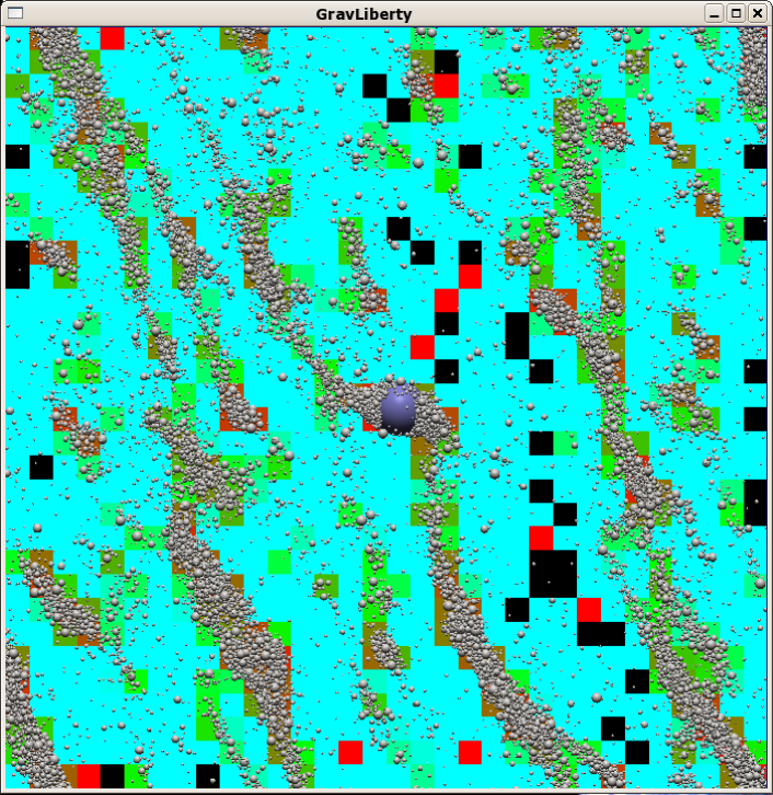
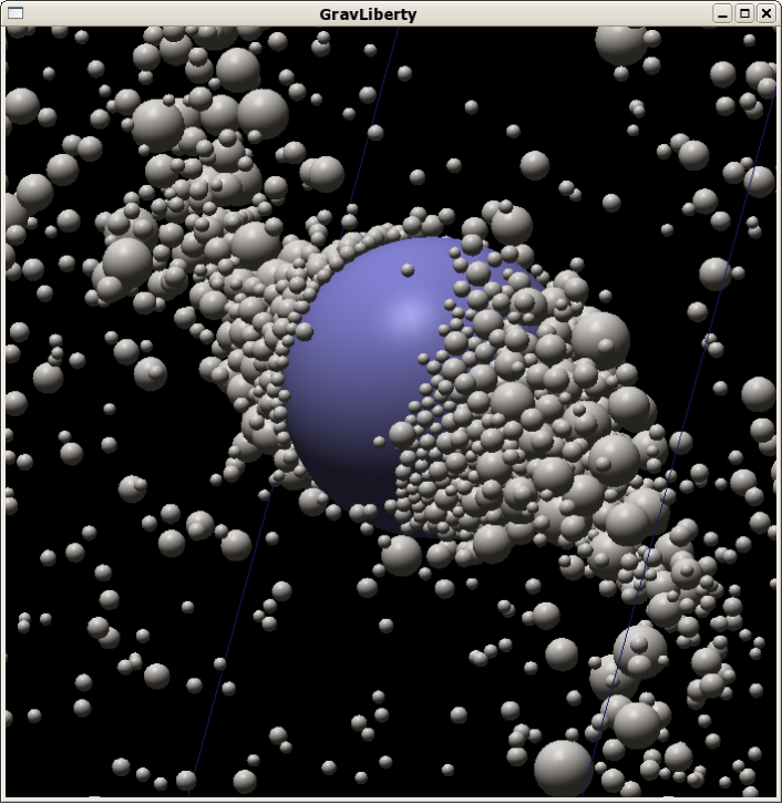
The visualisation of large data sets plays an increasingly important role in the scientific process. GravTree comes with a visualisation module, based on the OpenGL API. It can be used to visualise simulations in real time while they are running or in a standalone playback mode. The real time mode has proven to be especially useful during the development process.
Beside the particle distribution itself, average quantities such as the velocity dispersion and the filling factor can be shown as a transparent overlay. The tree structure can also be plotted. All graphic routines are easily expandable to incorporate any diagnostic that the current project requires. Two screenshots are shown in figures 7 and 8.
Chapter 12 Hydrodynamical simluations with Prometheus
Simulations of planets embedded in an accretion disc have been performed by a large number of authors in recent years. There are two main types of algorithm that can be used to simulate gas dynamics: finite difference methods such as ZEUS (Stone & Norman, 1992), NIRVANA (Ziegler & Yorke, 1997) and FARGO (Masset, 2000) or Godunov methods like RODEO (Paardekooper & Mellema, 2006) and ATHENA (Stone et al., 2008). As the name suggests, finite difference codes evaluate partial derivatives with a finite difference approximation. Godunov methods solve (exactly or approximately) a Riemann problem at every cell interface.
In this appendix, the code Prometheus is presented, which is a finite difference code in spherical coordinates, specialised for planet disc interactions. It is similar to the FARGO code but can also run simulations in three dimensions and has a module for solving the full MHD equations. This appendix can not be a comprehensive discussion of finite difference codes in general and merely lists the main concepts and implementation specific features of Prometheus.
Prometheus is written entirely in C and requires no external libraries. It can be compiled with a visualisation module, in which case it has to be linked to OpenGL, GLUT and libpng. Prometheus will be made publicly available at http://github.com/hannorein/prometheus.
Appendix 12.A Navier-Stokes equations
For many astrophysical processes collisions between gas particles are frequent enough such that a continuum description can be used. Here, the proto-planetary disc is treated as a gas whose motion is described by the Navier-Stokes equations. Although an MHD module has already been written for this code, it is not described here, due to current lack of testing and it has also not been used in scientific runs yet. We therefore restrict this discussion to the classical Navier-Stokes equations without magnetic fields, which we list in the following for both two and three dimensions.
1 Three dimensions
In spherical coordinates as defined in figure 1, the inviscid Navier-Stokes equations in conservative form are
| (1) | |||||||
| (2) | |||||||
| (3) | |||||||
| (4) | |||||||
Here, is the density, the velocity, the pressure and the acceleration due to the star, planets or other forces (e.g. from a rotating coordinate system). The terms on the left hand side describe advection, the terms on the right hand side are source terms. Equations 1-4 are the continuity equation, the radial momentum equation, the meridional momentum equation and the angular momentum equation, respectively. The system of equations is closed with an equation of state, determining the pressure . All simulations presented in this thesis use an isothermal equation of state , where the sound speed might vary with radius.
2 Two dimensions
One can simplify the equations in the previous section by averaging over the component, or for cylindrical coordinates, to obtain a two dimensional system of equations. The vertically averaged surface density is given as the integral over the density
| (5) |
Thus, in two dimensional polar coordinates the Navier-Stokes equations can be written as
| (6) | |||||||
| (7) | |||||||
| (8) | |||||||
Here, is the velocity two-vector , sometime also written as . Equation 6 is the two dimensional continuity equation, equation 7 is the radial momentum equation and equation 8 is the angular momentum equation.
In general the two dimensional system is a good approximation in planet disc simulations. In two dimensions, a smoothed planet potential is used to simulate the vertical structure of the circum-planetary disc (see equation 11). The smoothing length is approximately half the local disc scale height.
3 Viscosity
Strong physical viscosity is often used to model the effective viscosity resulting from turbulence (see section 1). This can be achieved by an additional source term in equations 1-4 and 7-8. Here, we restrict ourselves to the two dimensional case in which the additional terms to equations 7 and 8 are given by (see e.g. Masset, 2002)
| (9) | |||||
| (10) |
The components of the symmetric viscous stress tensor are given by
| (11) | |||||
| (12) | |||||
| (13) |
where we have used
| (14) | |||||
| (15) | |||||
| (16) |
Here, is the shear viscosity and the bulk viscosity has been assumed to be zero. can be expressed in terms of the parameter (Shakura & Syunyaev, 1973) via , with being the local sound speed and being the orbital period.
Appendix 12.B Discretisation
To solve equations 1-4 or 6-8 numerically, we discretise them on a grid. A staggered grid, where the velocities are face-centred and the densities are cell-centred has been used, as illustrated in the two dimensional case in figure 2. The discretisation is identical to that used in the ZEUS code. A staggered grid has the advantage that spacial derivatives are automatically second order accurate, but does also add some complexity, especially in three dimensions.
In the radial direction, the boundary conditions can be chosen to be either reflecting or damping. In the azimuthal direction, the boundary conditions are periodic. It is also possible to simulate only a wedge of the disc (without any planets). In three dimensions, periodic boundary conditions are used in the direction.
1 Operator splitting
Prometheus makes use of the operator splitting technique, where the equations are solved in small chunks. To do that, a time-step is divided into several sub-time-steps. Figure 3 illustrates the main loop in Prometheus, including the additional function calls for the MHD module, which are not discussed any further here.
First, the source terms (right hand side of equations 1-4 and 6-8) are added. Then, the advection terms (left hand side of equations 1-4 and 6-8) are solved using the half updated values after the source step, ignoring all terms on the right hand side. We further use dimensional splitting, solving the advection in the radial, azimuthal and meridional directions consecutively.
This method is only a simplified approximation to the real solution, but has proven to be more accurate than a single time-step. It is (approximately) second order accurate in time. Furthermore, it has the advantage that new physics can be easily incorporated as additional sub-time-steps. In this code we make use of this when an MHD module is added. However, operator splitting can also lead to spurious results in special circumstances, as shown in section 2.
2 Constrained transport
The transport step is solved using the integral representation of equations 1-4 and 6-8 to ensure conservation of mass and (angular-)momentum up to machine precision. We therefore need to have the fluxes at cell boundaries. There are different ways of estimating the cell faced, time centred flux at each interface, whose discussion goes beyond the scope of this section. In general, higher order methods are less diffusive but computationally more expensive. Both the first order donor cell method and the second order van Leer method have been implemented.
Additionally, a concept called constrained transport is used, where the momentum flux calculations are constrained, such that they are consistent with the mass flux. This leads to improved conservation properties. It is physically motivated, as all conserved quantities are advected by the fluid.
3 Splitting the angular momentum equation
Masset (2000) proposes a method, called FARGO (Fast Advection in Rotating Gaseous Objects), to speed up calculations in which there is a large mean background flow, as it is the case in a sheared accretion disc. The idea is to rewrite the advection terms, the second column in equations 1-4 and 6-8, by replacing the angular velocity by the sum . We choose to be the mean angular velocity of the annulus, rounded such that is an integer multiple of the grid spacing . is the remainder of the rounding operation and thus less or equal than . Both and are independent of and defined for an annulus with constant . The residual velocity is given by . Thus, the contribution from the component in a generic advection term of the form can be written as
| (17) |
where can be any quantity. The term (c) is just like the old advection term, but with a different velocity, as if we were in a rotating frame. The terms (a) and (b) can be interpreted as a simple shift. Because we’ve chosen such that is an integer multiple of the grid spacing , the term (a) corresponds to shifting the whole ring of cells, which is numerically very inexpensive. Because and the time-step constraint arising from the CFL condition allows us now to use much larger time-steps and the terms (b) and (c) can be solved using a standard advection algorithm. The splitting of the advection term gives an efficiency boost of a factor , in a typical simulation.
Appendix 12.C Tests
1 Shock-tube problems

Shock-tube problems are a standard test in numerical codes (see e.g. Stone & Norman, 1992). Even though these test are in general not very thorough and easy to pass, we present a one dimensional example in Cartesian geometry, mainly for comparison with a low Mach number shock in section 2.
The Mach number of the shock front is . An equidistantly spaced grid with 256 grid points, a CFL condition of 0.5 and a sound speed of is used. The density profile after together with the analytic solution is plotted in figure 4. One can see that the artificial viscosity smears out the discontinuity over several grid cells. Furthermore, the rarefaction wave results in some undershooting. These effects are expected and present in any finite difference code.
2 Dispersion error
Finite difference codes are known to have a numerical dispersion error because they do not, contrary to Godunov methods, solve the equations along wave characteristics. The fluid equations are solved using operator splitting. Each part, namely the source and transport step, are evaluated successively. Propagating sound waves involve both operators. The advection of a passive scalar, contrariwise, requires only one operator.
In most situations, this does not create any problems, as the error associated with the operator splitting is small and mostly affects the highest frequency modes which appear on the grid scale. However, if there is a discontinuity in the flow, large frequencies are present that can lead to a large dispersion error. For supersonic shocks, the artificial viscosity takes care of this, by smearing out discontinuities over a few grid cells, as shown in section 1. For low amplitude, subsonic shocks this might not be the case. The shock behaves like a travelling wave package, where the package includes a discontinuity.
Unfortunately, we are exactly in this situation for a low mass planet being embedded in an accretion disc. The wake of the planet contains a discontinuity and its amplitude depends on the planet’s mass. For sufficiently small masses, the discontinuity becomes subsonic and we expect noticeable numerical dispersion to occur. Since the wake is stationary in a frame co-rotating with the planet, the result will also be a stationary pattern.
In the following, we will first illustrate the problem with a shock tube test in a Cartesian box. We will then show that the same pattern appears in simulations of low mass planets and outline possible solutions such as physical viscosity and Godunov methods.
Low Mach number shock-tube tests
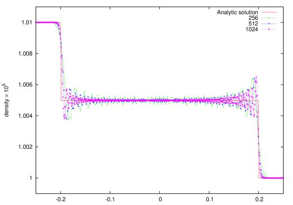
We set up a simple test problem that shows the problematic behaviour. We work in a Cartesian grid with resolutions 256x256, 512x512 and 1024x1024 and use an isothermal equation of state with sound speed in dimensionless units. The box has periodic boundary conditions and we set up a shock-tube problem by increasing the density in the left part of the box by 1%. The analytic solution after is plotted as a solid line in figure 5. Due to the low amplitude of the initial perturbation, the waves are basically sound packages travelling at the speed of sound, i.e. the rarefraction wave is very steep. Large ringing can be observed in the numerical solutions, which are also plotted in figure 5. This is because the numerical dispersion error is largest for the smallest wavelength. As expected for a Gibbs-like phenomenon, the over and under-shoots do not die out with increasing resolution. However, they get more concentrated near the discontinuity.
Note that in all simulations, the Neumann and Richtmyer artificial viscosity is switched on. The artificial viscosity does not kill the overshoots as it is quadratic in the velocities. This is reasonable approach in strong shocks (Stone & Norman, 1992, section 1). However, the velocity perturbations are very small compared to the sound speed in this case.
Low mass planets
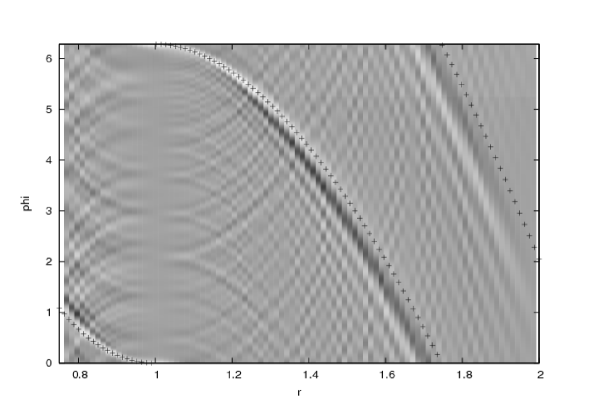
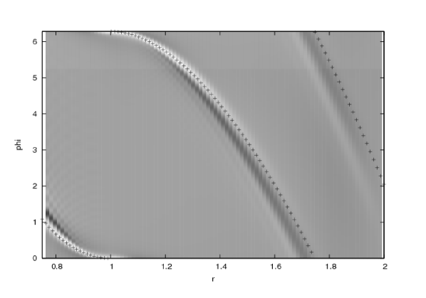
A similar phenomenon can be observed in simulations of planet disc interactions. All integrations were performed with Prometheus. The results have been confirmed with a variety of codes (FARGO, NIRVANA and RH2D) and do not depend on the implementation.
The phenomenon is stronger for low mass planets, as the shocks that appear in the wake are weaker and eventually become subsonic. Therefore, a planet with a very low mass of is used in these simulations. The cylindrical grid is spaced equidistantly in the radial direction and has a resolution of 128x384. We plot the surface density contours of one simulation with and without physical viscosity in figure 6. We over-plot the analytic position of the wake (Ogilvie & Lubow, 2002).
One can clearly see that there are over-shootings occurring, similar to those discussed above. Including a small amount of physical viscosity smears out the phenomenon. Increasing the resolution also helps to reduce the strength of the over-shootings. Numerical diffusion becomes more important if more grid cells, and therefore also a smaller time-step, are used.
For reasonable resolutions (), the torque on the planet is not significantly affected by this effect for two reasons. Firstly, the over-shootings appear a few scale heights away from the planet. Secondly, the gravitational torque from the over and under-shootings cancel and give almost no net effect. However, note that this is not necessarily the case for multi planetary systems or situations in which the saturation of co-rotation torques plays an important role (Paardekooper & Papaloizou, 2009). In those cases, finite difference codes should only be used with great care and possibly with explicit physical viscosity.
The phenomenon described here does not occur in Godunov codes such as RODEO (S.-J. Paardekooper, private communication). This is expected, as those schemes do solve the hydrodynamical equations along characteristics and therefore do not have a dispersion error.
3 Planet torques

As a further test, we calculate the torques for low mass planets in various disc models. A planet mass of and a smoothing length of is used, so that the simulations can be easily compared to those performed by Paardekooper & Papaloizou (2009). We first test the two dimensional version of Prometheus without physical viscosity. The specific torque felt by the planet is plotted in figure 7, normalised by the square of the planet mass ratio time the disc surface density for four different surface density profiles with slope . It can be seen by comparing figure 7 to figure 7 in Paardekooper & Papaloizou (2009) that the measured torques (and therefore the migration rates) are in very good agreement. In particular the case is in accord with linear theory (since it does not vary on a libration timescale). The long term trend visible towards the end of the simulation is due to different boundary conditions used (damping).
4 Planet disc interaction in three dimensions

We now go on and test a three dimensional simulation of planet disc interaction. Therefore, the results from Prometheus are compared to those of Kley et al. (2009).
A 20 Earth mass planet is set up on an eccentric and inclined orbit () and embedded in a stratified, three dimensional disc. The disc mass in the computational domain () is and the aspect ratio of the disc is 0.05. The grid resolution used is . We use no viscosity and a planet potential which is smoothed over a fraction (0.43) of a scale height. Note that this is a slightly different setup, compared to Kley et al. (2009).
Appendix 12.D Visualisations
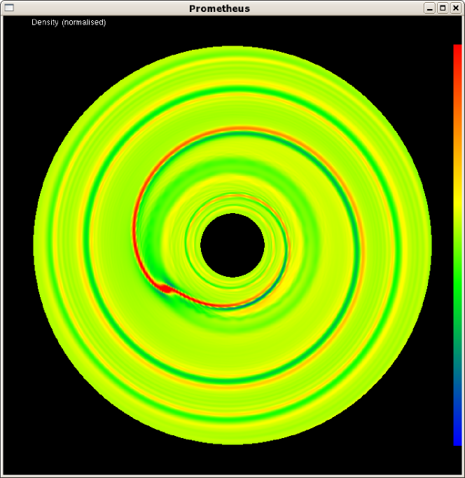
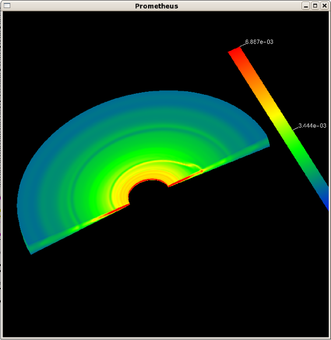
Similar to the visualisation module presented in appendix 11, Prometheus comes with a visualisation module, based on the OpenGL API. It can be used to visualise simulations in real time while they are running or in a standalone playback mode. Standard quantities, such as density, velocity, divergence of velocity and vorticity can be plotted in both, two and three dimensional simulations in either a cylindrical/spherical or Cartesian representation. Two screenshots are shown in figures 9 and 10.
The visualisation module is also easily adaptable to allow for direct user interaction with the simulation. For example, this can be used to add perturbations or additional planets to the simulation and watch the simulation change instantaneously. This provides an astonishing new way to easily understand physical phenomena.
Furthermore, an iPhone version of Prometheus is available on the Apple AppStore at http://itunes.apple.com/us/app/hydro/id341643251?mt=8.
References
- Adams & Bloch (2009) Adams, F. C. & Bloch, A. M. 2009, ApJ, 701, 1381
- Adams et al. (2008) Adams, F. C., Laughlin, G., & Bloch, A. M. 2008, ApJ, 683, 1117
- Alexander et al. (2006) Alexander, R. D., Clarke, C. J., & Pringle, J. E. 2006, MNRAS, 369, 229
- Anderson et al. (2010) Anderson, D. R., Hellier, C., Gillon, M., et al. 2010, ApJ, 709, 159
- Balbus & Hawley (1991) Balbus, S. A. & Hawley, J. F. 1991, ApJ, 376, 214
- Barge & Sommeria (1995) Barge, P. & Sommeria, J. 1995, A&A, 295, L1
- Barnes & Hut (1986) Barnes, J. & Hut, P. 1986, Nature, 324, 446
- Blum & Wurm (2008) Blum, J. & Wurm, G. 2008, ARA&A, 46, 21
- Bodenheimer & Pollack (1986) Bodenheimer, P. & Pollack, J. B. 1986, Icarus, 67, 391
- Bond et al. (2004) Bond, I. A., Udalski, A., Jaroszynski, M., et al. 2004, The Astrophysical Journal, 606, L155
- Boss (2001) Boss, A. P. 2001, ApJ, 563, 367
- Bridges et al. (1984) Bridges, F. G., Hatzes, A., & Lin, D. N. C. 1984, Nature, 309, 333
- Brouwer & Clemence (1961) Brouwer, D. & Clemence, G. M. 1961, Methods of celestial mechanics (New York: Academic Press, 1961)
- Chauvin et al. (2004) Chauvin, G., Lagrange, A.-M., Dumas, C., et al. 2004, A&A, 425, L29
- Chiang & Youdin (2009) Chiang, E. & Youdin, A. 2009, ArXiv e-prints
- Chiang & Goldreich (1997) Chiang, E. I. & Goldreich, P. 1997, ApJ, 490, 368
- Correia et al. (2008) Correia, A. C., Udry, S., Mayor, M., et al. 2008, å
- Cresswell & Nelson (2008) Cresswell, P. & Nelson, R. P. 2008, A&A, 482, 677
- Crida (2009) Crida, A. 2009, ApJ, 698, 606
- Crida et al. (2009) Crida, A., Baruteau, C., Kley, W., & Masset, F. 2009, A&A, 502, 679
- Crida et al. (2010) Crida, A., Papaloizou, J., Rein, H., Charnoz, S., & Salmon, J. 2010, AJ, submitted
- Crida et al. (2008) Crida, A., Sándor, Z., & Kley, W. 2008, A&A, 483, 325
- Cumming et al. (2008) Cumming, A., Butler, R. P., Marcy, G. W., et al. 2008, PASP, 120, 531
- Cuzzi et al. (1993) Cuzzi, J. N., Dobrovolskis, A. R., & Champney, J. M. 1993, Icarus, 106, 102
- Cuzzi et al. (2008) Cuzzi, J. N., Hogan, R. C., & Shariff, K. 2008, ApJ, 687, 1432
- Daisaka et al. (2001) Daisaka, H., Tanaka, H., & Ida, S. 2001, Icarus, 154, 296
- de Val-Borro et al. (2006) de Val-Borro, M., Edgar, R. G., Artymowicz, P., et al. 2006, MNRAS, 370, 529
- Desch (2007) Desch, S. J. 2007, ApJ, 671, 878
- Enoch et al. (2008) Enoch, M. L., Evans, II, N. J., Sargent, A. I., et al. 2008, ApJ, 684, 1240
- Fabrycky & Tremaine (2007) Fabrycky, D. & Tremaine, S. 2007, ApJ, 669, 1298
- Fehlberg (1969) Fehlberg, E. 1969, Low-order Classical Runge-Kutta Formulas with Stepsize Control and Their Application to Some Heat Transfer Problems (NASA)
- Fromang & Papaloizou (2006) Fromang, S. & Papaloizou, J. 2006, A&A, 452, 751
- Fromang & Papaloizou (2007) Fromang, S. & Papaloizou, J. 2007, A&A, 476, 1113
- Fromang et al. (2007) Fromang, S., Papaloizou, J., Lesur, G., & Heinemann, T. 2007, A&A, 476, 1123
- Gammie (1996) Gammie, C. F. 1996, ApJ, 457, 355
- Goldreich (1965) Goldreich, P. 1965, MNRAS, 130, 159
- Goldreich & Tremaine (1979) Goldreich, P. & Tremaine, S. 1979, ApJ, 233, 857
- Goldreich & Tremaine (1980) Goldreich, P. & Tremaine, S. 1980, ApJ, 241, 425
- Goldreich & Tremaine (1982) Goldreich, P. & Tremaine, S. 1982, ARA&A, 20, 249
- Goldreich & Ward (1973) Goldreich, P. & Ward, W. R. 1973, ApJ, 183, 1051
- Hayashi (1981) Hayashi, C. 1981, Progress of Theoretical Physics Supplement, 70, 35
- Hayashi et al. (1977) Hayashi, C., Nakazawa, K., & Adachi, I. 1977, PASJ, 29, 163
- Ida & Lin (2004) Ida, S. & Lin, D. N. C. 2004, ApJ, 604, 388
- Johansen et al. (2006) Johansen, A., Henning, T., & Klahr, H. 2006, ApJ, 643, 1219
- Johansen et al. (2007) Johansen, A., Oishi, J. S., Low, M.-M. M., et al. 2007, Nature, 448, 1022
- Johansen et al. (2009) Johansen, A., Youdin, A., & Mac Low, M. 2009, ApJ, 704, L75
- Kalas et al. (2008) Kalas, P., Graham, J. R., Chiang, E., et al. 2008, Science, 322, 1345
- Kasdin (1995) Kasdin, N. J. 1995, Proceedings of the IEEE, 83
- Kipping et al. (2009) Kipping, D. M., Fossey, S. J., & Campanella, G. 2009, MNRAS, 400, 398
- Kley et al. (2009) Kley, W., Bitsch, B., & Klahr, H. 2009, A&A, 506, 971
- Kley et al. (2004) Kley, W., Peitz, J., & Bryden, G. 2004, A&A, 414, 735
- Knutson et al. (2007) Knutson, H. A., Charbonneau, D., Allen, L. E., et al. 2007, Nature, 447, 183
- Konacki et al. (2003) Konacki, M., Torres, G., Jha, S., & Sasselov, D. D. 2003, Nature, 421, 507
- Laughlin et al. (2004) Laughlin, G., Steinacker, A., & Adams, F. C. 2004, ApJ, 608, 489
- Lee & Peale (2001) Lee, M. H. & Peale, S. J. 2001, in Bulletin of the American Astronomical Society, Vol. 33, Bulletin of the American Astronomical Society, 1198
- Lee & Peale (2002) Lee, M. H. & Peale, S. J. 2002, ApJ, 567, 596
- Lesur & Papaloizou (2009) Lesur, G. & Papaloizou, J. C. B. 2009, ArXiv e-prints
- Lewis & Stewart (2009) Lewis, M. C. & Stewart, G. R. 2009, Icarus, 199, 387
- Lin & Papaloizou (1986) Lin, D. N. C. & Papaloizou, J. 1986, ApJ, 309, 846
- Lucy (1977) Lucy, L. B. 1977, AJ, 82, 1013
- Lyra et al. (2009) Lyra, W., Johansen, A., Klahr, H., & Piskunov, N. 2009, A&A, 493, 1125
- Malhotra (1993) Malhotra, R. 1993, Icarus, 106, 264
- Masset (2000) Masset, F. 2000, A&AS, 141, 165
- Masset & Snellgrove (2001) Masset, F. & Snellgrove, M. 2001, MNRAS, 320, L55
- Masset (2002) Masset, F. S. 2002, A&A, 387, 605
- Masset & Papaloizou (2003) Masset, F. S. & Papaloizou, J. C. B. 2003, ApJ, 588, 494
- Mayor et al. (2009) Mayor, M., Bonfils, X., Forveille, T., et al. 2009, A&A, 507, 487
- Mayor & Queloz (1995) Mayor, M. & Queloz, D. 1995, Nature, 378, 355
- Michikoshi et al. (2007) Michikoshi, S., Inutsuka, S.-i., Kokubo, E., & Furuya, I. 2007, ApJ, 657, 521
- Michikoshi et al. (2009) Michikoshi, S., Kokubo, E., & Inutsuka, S.-i. 2009, ApJ, 703, 1363
- Mizuno (1980) Mizuno, H. 1980, Progress of Theoretical Physics, 64, 544
- Morishima & Salo (2006) Morishima, R. & Salo, H. 2006, Icarus, 181, 272
- Murray & Dermott (2000) Murray, C. D. & Dermott, S. F. 2000, Solar System Dynamics (Cambridge University Press)
- Nagasawa et al. (2008) Nagasawa, M., Ida, S., & Bessho, T. 2008, ApJ, 678, 498
- Nelson (2005) Nelson, R. P. 2005, A&A, 443, 1067
- Nelson & Papaloizou (2002) Nelson, R. P. & Papaloizou, J. C. B. 2002, MNRAS, 333, L26
- Nelson & Papaloizou (2004) Nelson, R. P. & Papaloizou, J. C. B. 2004, MNRAS, 350, 849
- Nelson et al. (2000) Nelson, R. P., Papaloizou, J. C. B., Masset, F., & Kley, W. 2000, MNRAS, 318, 18
- Ogilvie & Lubow (2002) Ogilvie, G. I. & Lubow, S. H. 2002, MNRAS, 330, 950
- Oishi et al. (2007) Oishi, J. S., Mac Low, M.-M., & Menou, K. 2007, ApJ, 670, 805
- Paardekooper et al. (2010) Paardekooper, S., Baruteau, C., Crida, A., & Kley, W. 2010, MNRAS, 401, 1950
- Paardekooper & Mellema (2006) Paardekooper, S. & Mellema, G. 2006, A&A, 450, 1203
- Paardekooper & Papaloizou (2009) Paardekooper, S. & Papaloizou, J. C. B. 2009, MNRAS, 394, 2283
- Papaloizou (2003) Papaloizou, J. C. B. 2003, Celestial Mechanics and Dynamical Astronomy, 87, 53
- Papaloizou & Szuszkiewicz (2005) Papaloizou, J. C. B. & Szuszkiewicz, E. 2005, MNRAS, 363, 153
- Papaloizou & Terquem (1999) Papaloizou, J. C. B. & Terquem, C. 1999, ApJ, 521, 823
- Papaloizou & Terquem (2006) Papaloizou, J. C. B. & Terquem, C. 2006, Reports of Progress in Physics, 69, 119
- Pepliński et al. (2008a) Pepliński, A., Artymowicz, P., & Mellema, G. 2008a, MNRAS, 386, 164
- Pepliński et al. (2008b) Pepliński, A., Artymowicz, P., & Mellema, G. 2008b, MNRAS, 386, 179
- Pepliński et al. (2008c) Pepliński, A., Artymowicz, P., & Mellema, G. 2008c, MNRAS, 387, 1063
- Pierens & Nelson (2008) Pierens, A. & Nelson, R. P. 2008, A&A, 482, 333
- Pollack et al. (1996a) Pollack, J. B., Hubickyj, O., Bodenheimer, P., et al. 1996a, Icarus, 124, 62
- Pollack et al. (1996b) Pollack, J. B., Hubickyj, O., Bodenheimer, P., et al. 1996b, Icarus, 124, 62
- Porco et al. (2007) Porco, C. C., Thomas, P. C., Weiss, J. W., & Richardson, D. C. 2007, Science, 318, 1602
- Press et al. (1992) Press, W. et al. 1992, Numerical recipes in C (Cambridge University Press Cambridge)
- Pringle (1981) Pringle, J. E. 1981, ARA&A, 19, 137
- Quinn et al. (2010) Quinn, T., Perrine, R. P., Richardson, D. C., & Barnes, R. 2010, AJ, 139, 803
- Rein & Papaloizou (2009) Rein, H. & Papaloizou, J. C. B. 2009, A&A, 497, 595
- Rein et al. (2010) Rein, H., Papaloizou, J. C. B., & Kley, W. 2010, A&A, 510, A260000+
- Rivera et al. (2005) Rivera, E. J., Lissauer, J. J., Butler, R. P., et al. 2005, ApJ, 634, 625
- Sándor & Kley (2006) Sándor, Z. & Kley, W. 2006, A&A, 451, L31
- Sano et al. (2000) Sano, T., Miyama, S. M., Umebayashi, T., & Nakano, T. 2000, ApJ, 543, 486
- Sasselov & Lecar (2000) Sasselov, D. D. & Lecar, M. 2000, ApJ, 528, 995
- Schmidt et al. (2009) Schmidt, J., Ohtsuki, K., Rappaport, N., Salo, H., & Spahn, F. 2009, Dynamics of Saturn’s Dense Rings (Springer), 413–458
- Schneider (2010) Schneider, J. 2010, http://exoplanet.eu
- Seiß et al. (2005) Seiß, M., Spahn, F., Sremčević, M., & Salo, H. 2005, Geophys. Res. Lett., 32, 11205
- Shakura & Syunyaev (1973) Shakura, N. I. & Syunyaev, R. A. 1973, A&A, 24, 337
- Sinclair (1975) Sinclair, A. T. 1975, MNRAS, 171, 59
- Snellgrove et al. (2001) Snellgrove, M. D., Papaloizou, J. C. B., & Nelson, R. P. 2001, A&A, 374, 1092
- Spahn & Sremčević (2000) Spahn, F. & Sremčević, M. 2000, A&A, 358, 368
- Sremčević et al. (2002) Sremčević, M., Spahn, F., & Duschl, W. J. 2002, MNRAS, 337, 1139
- Stewart & Leinhardt (2009) Stewart, S. T. & Leinhardt, Z. M. 2009, ApJ, 691, L133
- Stoer & Bulirsch (2002) Stoer, J. & Bulirsch, R. 2002, Introduction to Numerical Analysis (Springer)
- Stone et al. (2008) Stone, J. M., Gardiner, T. A., Teuben, P., Hawley, J. F., & Simon, J. B. 2008, ApJS, 178, 137
- Stone & Norman (1992) Stone, J. M. & Norman, M. L. 1992, ApJS, 80, 753
- Tanaka et al. (2002) Tanaka, H., Takeuchi, T., & Ward, W. R. 2002, ApJ, 565, 1257
- Tanga et al. (2004) Tanga, P., Weidenschilling, S. J., Michel, P., & Richardson, D. C. 2004, A&A, 427, 1105
- Tiscareno et al. (2008) Tiscareno, M. S., Burns, J. A., Hedman, M. M., & Porco, C. C. 2008, AJ, 135, 1083
- Tiscareno et al. (2006) Tiscareno, M. S., Burns, J. A., Hedman, M. M., et al. 2006, Nature, 440, 648
- Tiscareno et al. (2010) Tiscareno, M. S., Burns, J. A., Sremcevic, M., et al. 2010, in Bulletin of the American Astronomical Society, Vol. 41, Bulletin of the American Astronomical Society, 939–+
- Toomre (1964) Toomre, A. 1964, ApJ, 139, 1217
- Vogt et al. (2005) Vogt, S. S., Butler, R. P., Marcy, G. W., et al. 2005, ApJ, 632, 638
- Ward (1997) Ward, W. R. 1997, Icarus, 126, 261
- Weidenschilling (1977a) Weidenschilling, S. J. 1977a, MNRAS, 180, 57
- Weidenschilling (1977b) Weidenschilling, S. J. 1977b, Ap&SS, 51, 153
- WGESP (2003) WGESP. 2003, http://www.dtm.ciw.edu/boss/definition.html
- Wisdom & Tremaine (1988) Wisdom, J. & Tremaine, S. 1988, AJ, 95, 925
- Wolszczan & Frail (1992) Wolszczan, A. & Frail, D. A. 1992, Nature, 355, 145
- Wuchterl (1993) Wuchterl, G. 1993, Icarus, 106, 323
- Youdin & Goodman (2005) Youdin, A. N. & Goodman, J. 2005, ApJ, 620, 459
- Ziegler & Yorke (1997) Ziegler, U. & Yorke, H. W. 1997, Computer Physics Communications, 101, 54