Modeling and Analysis of Time-Varying Graphs

Abstract

We live in a world increasingly dominated by networks – communications, social, information, biological etc. A central attribute of many of these networks is that they are dynamic, that is, they exhibit structural changes over time. While the practice of dynamic networks has proliferated, we lag behind in the fundamental, mathematical understanding of network dynamism. Existing research on time-varying graphs ranges from preliminary algorithmic studies (e.g., Ferreira’s work on evolving graphs) to analysis of specific properties such as flooding time in dynamic random graphs. A popular model for studying dynamic graphs is a sequence of graphs arranged by increasing snapshots of time. In this paper, we study the fundamental property of reachability in a time-varying graph over time and characterize the latency with respect to two metrics, namely store-or-advance latency and cut-through latency. Instead of expected value analysis, we concentrate on characterizing the exact probability distribution of routing latency along a randomly intermittent path in two popular dynamic random graph models. Using this analysis, we characterize the loss of accuracy (in a probabilistic setting) between multiple temporal graph models, ranging from one that preserves all the temporal ordering information for the purpose of computing temporal graph properties to one that collapses various snapshots into one graph (an operation called smashing), with multiple intermediate variants. We also show how some other traditional graph theoretic properties can be extended to the temporal domain. Finally, we propose algorithms for controlling the progress of a packet in single-copy adaptive routing schemes in various dynamic random graphs.

1 Introduction

We live in a world increasingly dominated by networks – communications, social, biological etc – imagine, for instance, an ad hoc infrastructureless communications network of constantly mobile soldiers. A central feature of many of these networks is that they are dynamic, that is, they exhibit structural changes over time. While the practice of dynamic networks has proliferated, especially in the area of military communications networks, we lag behind in the fundamental, mathematical understanding of network dynamism.

Time-varying graphs have been a topic of active research recently [12, 9, 5, 19]. They are useful in the study of communication networks with intermittent connectivity such as delay-tolerant networks [15] and even disruption-tolerant social networks [14]; duty cycling wireless sensor networks [3, 7, 4], and the like. Existing research on time-varying graphs ranges from algorithmic studies on graph journeys  [12] to analysis of specific properties such as flooding time in dynamic random graphs [9, 5]. Empirical simulation-based analysis of certain temporal graph properties such as temporal distance and temporal efficiency has also been a topic of recent research [21].

In this paper, we propose a model of time-varying graphs called Temporal Graphlets which are essentially a time-series of static graph snapshots. While similar models have been studied in the literature before, albeit with alternative names such as space-time graphs [18], we propose new research directions in temporal graph theory and present analytical results on two different aspects of this temporal graph model.

First, a directed stacked graph is created from all the temporal snapshots of the time-varying graph and we show how certain standard graph theoretic properties such as reachability, connectivity, etc. can be extended to this model. Then we propose a technique named smashing for collapsing all or parts of the temporal graph and analyze how the reachability property is affected due to the loss of temporal ordering information. We also introduce an intermediate model of $m$-smashed graphs which selectively collapse parts of the temporal graph while preserving the remaining stacked structure. We show how the degree of smashing can impact graph properties by means of a thorough comparative probabilistic analysis of the reachability property for the simple time-varying line network. This is potentially useful for online analysis of large temporal graphs where accuracy can be traded for speed and complexity.

We study two different metrics for measuring latency in this paper: (a) Store-or-advance; and (b) Cut-through. In the former, a message can be forwarded to only a neighbor in a unit time step, whereas in the latter, a message can be routed to any neighbor in the currently connected component instantaneously. In this paper, we study theoretical aspects of reachability in temporal graphs under various random edge-dynamics models. In particular, we characterize the exact probability distributions for latency (not just the first moment) and also a recursive form for message location in two popular dynamic random graph models for the dynamic line graph (or linear network topology), namely, the independent probabilistic model and the two-step Markov chain model.

Finally, we propose an adaptive routing algorithm that minimizes expected traversal time between a source and a destination node in the independent probabilistic temporal graph model.

This paper is organized as follows. Section 2 introduces deterministic and random models of temporal graphs. Section 3 presents results on the probabilistic analysis of latency along dynamically changing random paths in graphs. Section 4 presents stacked and smashed graph models for temporal graphs and presents comparative probabilistic analysis of latency under both models for time-varying random paths. Section 5 presents an adaptive routing algorithm in time-varying graphs. Section 6 concludes the paper with a discussion on future research directions.

2 Models of Temporal Graphs

Time-varying graphs occur commonly in the real world, and it is necessary to have mathematical models for their representation. We first introduce a deterministic model for representing a series of time-varying graphs, and propose two different models for routing in such graphs. We then propose enhancements to well known dynamic random graph models, which are used throughout this paper for analysis.

2.1 Temporal Graphlets: A Deterministic Model of Dynamic Graphs

Assume slotted time starting at time $0$. Slot $t$ starts just after time $t-1$ and ends at time $t$. A Temporal Graphlet Sequence $TGS(T_{1},T_{2})=\{G(t)=(V(t),E(t))\},T_{1}\leq t\leq T_{2}$ is our basic deterministic model for a dynamic network and attempts to capture its space-time trajectory (see Figure 1). Each $G(t)$ is referred to as a Temporal Graphlet or simply Graphlet. Alternate notations that we will use, depending on the emphasis, include $G(T_{1},T_{2})$, $G[1,T]$ (shifting the frame of reference maintains properties), $G[T]$ (reference shifting is implied).

While traditional graph theory only considers properties in the “horizontal” (space) dimension, we consider properties across the “vertical” (time) dimension as well. For instance, $u\rightarrow v$ is $T$-reachable iff there exists a sequence of edges $(u_{1},u_{2}),(u_{2},u_{3}),...(u_{m-1},u_{m})$, $u=u_{1}$, $v=u_{m}$ and $(u_{i},u_{i+1})$ $\in$ $V(t_{j})$, $1\leq i<m$, $t_{j}\geq t_{j-1}$, $1\leq t_{j}\leq T$.

For example, in Figure 1, every graphlet is disconnected, but T-reachability holds for $a\rightarrow f$. Similarly, a T-cut is the removal of a set of vertices $X\subset V(1)\cup V(2)\cup V(3)\ldots\cup V(t)$ that results in some $u$ and $v$ losing their T-reachability property. Special or restricted temporal graphlets are also possible, e.g., a T-$k$-regular graph is one in which every node makes unique contact exactly $k$ times during its lifetime.

Assume a node $v$ wants to send a message to a certain node $u$. At the beginning of a slot the node that has the message can store it or forward it to another neighboring node. At the end of the slot the graph may change according to the TGS. There are two models for measuring progress accomplished by a message under the circumstances.

Definition 2.1.

In the Store or Advance (SoA) model, a node can forward the message only to one of its direct neighbors, and that is assumed to take a time slot. Even if the neighbor’s neighboring edges are active right now, one may not be able to avail those edges right away. Instead, one has to wait for at least one (generally more) time slot(s) until the message reaches the neighbor.

Definition 2.2.

In the Cut-through (CuT) model, a node may send the message to any node in its connected component, and the entire connected component can be traversed instantaneously or at least in a much shorter time scale than that of edge dynamics.

While the SoA model finds more applications in most time-varying networks such as MANETs, DTNs, and social networks [14], the CuT model is interesting in its own right, and has been proposed in certain applications in low latency MANET design [20].

Figure 1: Temporal Graphlets for $t$ = 1,2,3. $V(1)=V(2)=V(3)$ = {a,b,c,d,e,f}. Although this figure does not illustrate it, vertex set need not be the same (nodes could be added or deleted)

In Section 4, we show how the deterministic temporal graphlet model can be useful for extending static graph theoretic properties to dynamic graphs. A related concept of slices has been proposed recently [19]. They define coupling variables between instances of the same node in consecutive slices. However, the focus of this work is on detecting communities over time.

2.2 Stochastic Models of Dynamic Graphs

Random graph models are very useful for studying a plethora of graph properties in a probabilistic sense. A classic example of random graphs is the family of Erdos-Renyi graphs $ER(n,p)$ which are static graphs on $n$ nodes with any of the $n\choose 2$ edges existing with probability $p$. The probability of the existence of an edge is independent of that of another edge in the graph. Although too simplistic and perhaps unrealistic for many application scenarios, random graphs have played a big role in the development of a good understanding of key physical phenomena such as phase transitions and percolation [13].

Researchers have proposed adding a time dimension to the static random graph model such that time is slotted and each edge in the graph exists in each time slot with probability $p$ and does not exist with probability $1-p$ [10]. We refer to this graph as the dynamic Erdos-Renyi graph.

Definition 2.3.

Dynamic $ER(p)$ graphs: $G_{t}$ which is the graph at the end of slot $t$ and at the beginning of slot $t+1$ is drawn from the family of graphs $ER(n,p)$. $G_{0}$ is the initial graph and $G_{T}$ is the final graph if the time horizon ends at time $T$.

Definition 2.4.

Markovian $(q,p)$ graphs: In this model of dynamic random graphs [9], each edge in $G_{t}$ can be in one of two states, ON or OFF, and the probability distribution is governed by a two-state Markov chain. The transition probabilities are given by $P(OFF\rightarrow ON)=p$, $P(OFF\rightarrow OFF)=1-p$, $P(ON\rightarrow OFF)=q$, and $P(ON\rightarrow ON)=1-q$.

We propose a generic enhancement to these two dynamic random graph models. Instead of allowing a stochastic process to act on all of the possible $n\choose 2$ edges, we restrict it to act on only the edges in a given underlying graph, $G_{u}$. Clearly, when $G_{u}=K_{n}$, the complete graph, these stochastic process applies to all possible edges, and then this is equivalent to the older model.

Observation 2.1.

The Markov $(1,1)$ dynamic graph corresponds to the family of perfectly alternating graphs, $(G_{t},G_{t+1})$, such that $G_{t+1}$ has all the edges that do not exist in $G_{t}$, and vice versa.

Observation 2.2.

At any time slot, if $G_{u}=K_{n}$, the $(1-p,p)$ Markov graph is equivalent to the dynamic $ER(p)$ graph.

Observation 2.3.

Another special case is the $(p,p)$-stochastic model. Here, define $p$ to be the stability factor. For small $p$, there are few changes from $G_{t}$ to $G_{t+1}$ and the graph is stable. For large $p$, there could be many changes from $G_{t}$ to $G_{t+1}$ and the graph is unstable. A special case of this special case is the $(1,1)$-stochastic model in which edges and non-edges alternate at each time slot.

3 Analyzing Latency along Dynamic Paths

Many routing schemes determine a path (say, according to a shortest path calculation), and then stay on that path even though it may be intermittently connected due to edges on it appearing and disappearing according to one of the aforementioned stochastic processes.

Hence we consider the simplest case which is amenable to mathematical analysis – the underlying graph $G_{u}=L_{n}$, the line graph with $n$ vertices and $n-1$ edges in which vertex $1$ wants to send a message to vertex $n$. We denote these graphs by $ER(n,p,L_{n})$ and $MC(q,p,L_{n})$. Clearly a message should either be stored or be either advanced as much as possible (under the CuT model) or one hop per time slot (under the SoA model).

We now study how random variables such as time taken to reach node $n$ from node $1$ behave as a function of $n,p,q,G_{u}$. We first show how simple expected value analysis can yield first moments, and then characterize the entire probability distributions as a function of such parameters. The results of this analysis will be applicable to the analysis of Temporal Graphlets in Section 4.

3.1 The $(1,1)$-Stochastic Model

For the $(1,1)$-stochastic model, one can compute the exact arrival time. Define a configuration as a binary string of length $n-1$. If the $i$-th bit is $1$ then the $i$-th edge on the line exists otherwise it does not exist. For a given binary string $B$, let $k(B)$ be the number of changes from $0$ to $1$ or from $1$ to $0$ and let $b(B)$ be the value of the first bit of $B$. For example, $k(001110011001)=5$.

Observation 3.1.

The routing in the CuT model takes $k+1-b$ slots.

Observation 3.2.

The routing in the SoA model takes $2n-k-b$ slots.

Corollary 3.1.

The best configuration for CuT is $111\cdots 1$ for which the routing takes $0$ slot

Corollary 3.2.

The worst configuration for CuT is $0101\cdots$ for which the routing takes $n-1$ slots.

Corollary 3.3.

The best configuration for SoA is $1010\cdots$ for which the routing takes $n-1$ slots.

Corollary 3.4.

The worst configuration for SoA is $000\cdots 0$ for which the routing takes $2(n-1)$ slots.

We now compute the average routing time assuming a uniform distribution for all the $2^{n-1}$ configurations.

Observation 3.3.

The average routing time for CuT is $\frac{1}{2}(n-1)$ slots.

Observation 3.4.

The average routing time for SoA is $\frac{3}{2}(n-1)$ slots.

3.2 The $(1-p,p)$-Stochastic Model

This is equivalent to the $ER(n,p,L_{n})$ model. We first begin with computation of expected values of advancement of a message until it hits a non-edge and the expected routing latency. Subsequently we derive the exact probability distributions of the spatio-temporal location of the message as well the distribution of the routing latency under both the SoA and CuT models.

Observation 3.5.

In SoA the expected advance is $p\cdot 1+(1-p)\cdot 0=p$.

Observation 3.6.

In CuT the expected advance is upper-bounded by $(1-p)\sum_{i=1}^{\infty}ip^{i}=\frac{p}{1-p}$.

The following corollaries follows since the length of the route is $n-1$.

Corollary 3.5.

In SoA the expected time for the routing time is $\frac{n-1}{p}$.

Corollary 3.6.

In CuT the expected time for the routing time is $\frac{(n-1)(1-p)}{p}$.

SoA latency

Consider an Erdos-Renyi line graph on $n$ nodes which denoted by $ER^{t}(n,p,L_{n})$ at the $t$-th time instant. There are a maximum of $n-1$ edges in this graph, and at each time instant, each edge exists with probability $p$. We want to send a packet from node $1$ to node $n$; if an edge $(u,v)$ is up at time instant $t$, and $u$ has the packet, then it will transmit to $v$ in that instant, otherwise, it will hold it until a later time instant when the edge becomes active. We want to track the probability distribution of the packet over time as a function of $n$ and $p$.

Let $N_{t}$ be a random variable denoting the node that the packet has reached at time $t$, and $e_{k}$ be the $k$-th edge.

$$P(N_{t}=k) = P(N_{t-1}=k-1)P(e_{k-1})+P(N_{t-1}=k)P(\overline{e_{k}})$$ (1)

$$= P(N_{t-1}=k-1)p+P(N_{t-1}=k)(1-p)$$

It is difficult to solve the above bivariate recurrence to attain a closed form for $P(N_{t}=k)$, hence we compute the probabilities numerically. Figure 2 shows an example of a probability distribution for a small line graph. The example considers a line graph on $n=10$ nodes for $p=0.25$. It is easy to see that since the expected waiting time for every hop is $\frac{1}{p}$, each hop takes approximately 4 time slots to traverse. Hence at $t=20$, the packet would have traversed a mean of 5 hops, which is indicated in the figure.

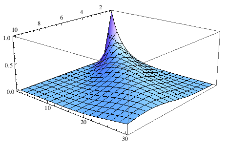
Figure 2: Probability distribution of the packet as function of space and time for $ER(n=10,p=0.25,L_{n})$ for $t=30$

Let $T$ be a random variable denoting the number of time slots needed for a packet to reach from node $1$ to node $n$. It is easy to see that $P(T<n-1)=0$ since it takes at least $n-1$ slots to reach node $n$. The general distribution of $T$ is given by the following:

$$P(T=n-1+j)={n+j-2\choose j}(1-p)^{j}p^{n-1},\forall{j}\geq 0$$ (2)

This is because there are exactly $j$ time slots when the packet has to wait at one of the nodes $1,2,3,\ldots,n-1$, and there are ${n+j-2\choose j}$ number of ways of assigning these $j$ slots to the $n-1$ nodes. Figure 3 plots this distribution.

It can easily be verified that $E[T]=\sum_{k=0}^{\infty}kP(T=k)=\frac{n-1}{p}$, which is in agreement with Corollary 3.5.

CuT latency

We now characterize the distribution of routing times in terms of the cut-through metric. It is assumed that the time taken to cut through the edges in a connected component do not cost any time slots and time elapses only due to waiting for an inactive link to become active.

Let $T$ be the random variable denoting the number of time slots taken to reach node $n$ from node $1$ if nodes were forwarding the packet as much as possible toward the destination in the current connected component.

$$P(T=k) = Pr\{\textrm{Wait for $k$ slots at $\{1,2,\ldots,n-1\}$}\}$$ (3)

$$= {n+k-2\choose k}(1-p)^{k}p^{n-1}$$

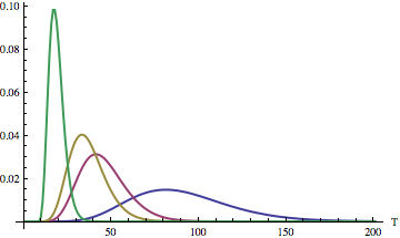
Figure 3: Probability distribution of time taken to traverse the dynamic line graph $ER(10,p,L_{10})$ for values of $p=\{0.1,0.2,0.25,0.5\}$

This is because the number of ways of assigning $k$ waiting slots at one or more of nodes $\{1,2,\ldots,n-1\}$ is the same as number of ways putting $k$ balls in $n-1$ distinct bins with no restrictions on the number of balls in a particular bin, and this is given by ${n+k-2\choose k}$. Note that the only reason the packet needs to wait for a slot at node $j$ is if the edge $(j,j+1)$ is inactive at that time instant. This contributes to the $p^{k}$ term.

It can be verified that $E[T]=\sum_{k=0}^{\infty}kP(T=k)=(n-1)\frac{1-p}{p}$, which is consistent with Corollary 3.6. Also, the variance is given by: $Var[T]=E[T^{2}]-E[T]^{2}=(n-1)\frac{1-p}{p^{2}}$. Not surprisingly the mean time elapsed when using the CuT metric is smaller than that in case of the SoA metric.

3.3 The $(q,p)$-Markov Model

Now we study routing on dynamic line graphs $MC(p_{0},q,p,L_{n})$, where $p_{0}$ is the probability of an edge existing in the first graphlet.

Observation 3.7.

It is easy to see that this Markov chain has a stationary distribution $\pi=(\pi_{on},\pi_{off})=(\frac{p}{p+q},\frac{q}{p+q})$. To eliminate the effect of transients, we assume that the Markov chain has converged (or mixed) before node $1$ sends the message to node $n$; in other words, $p_{0}=\pi_{on}=\frac{p}{p+q}$.

Observation 3.8.

In CuT the expected advance on an infinite line is upper-bounded by $\frac{p}{q}$.

Observation 3.9.

In SoA the expected advance is $\frac{p}{p+q}$.

Corollary 3.7.

In CuT the expected time for the routing time is $\frac{(n-1)q}{p(p+q)}$. [Proof omitted]

Corollary 3.8.

In SoA the expected time for the routing time is $n-1+\frac{(n-1)q}{p(p+q)}$. [Proof omitted]

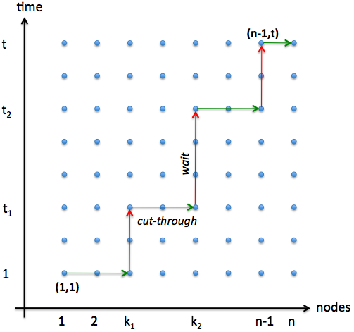
Figure 4: Analyzing the CuT latency in a dynamic random line graph

CuT latency

Figure 4 illustrates a sample path from $1\rightarrow n$ over time. There are several such paths possible depending on the state of the edges, and the computation here is more involved than the $ER(n,p,L_{n})$ case.

Any path through this space-time can be characterized by its constituent segments: $\{1,k_{1},t_{1},k_{2},t_{2},\ldots,k_{m},t_{m},n\}$, where $t_{m}=t$. Clearly $1\leq m\leq\min(n-1,t-2)$.

Let $X_{\tau}^{e}$ correspond to a binary random variable that denotes the status of edge $e$ at time instant $\tau$. The probability that path $P=\{1,k_{1},t_{1},k_{2},t_{2},\ldots,k_{m},t_{m},n\}$ exists is given by the following:

$$Pr\{P\} = Pr\{X_{1}^{1},X_{1}^{2},\ldots,X_{1}^{k_{1}-1},\overline{X}_{1}^{k_{1}},\overline{X}_{2}^{k_{1}},\ldots,\overline{X}_{t_{1}-1}^{k_{1}},X_{t_{1}}^{k_{1}},$$ (6)

$$\ldots,X_{t}^{k_{m}},\ldots,X_{t}^{n-1}\}$$

$$= P(X_{1}^{1})\cdots P(X_{1}^{k_{1}-1})P(\overline{X}_{1}^{k_{1}},\overline{X}_{2}^{k_{1}},\ldots,\overline{X}_{t_{1}-1}^{k_{1}},X_{t_{1}}^{k_{1}})$$

$$\cdots P(X_{t}^{k_{m}})P(X_{t}^{n-1})$$

$$= \pi_{on}^{k_{1}-1}\pi_{off}(1-p)^{t_{1}-2}p\times$$

$$\pi_{on}^{k_{2}-k_{1}-1}\pi_{off}(1-p)^{t_{2}-t_{1}-1}p\times$$

$$\cdots\pi_{on}^{n-k_{m}-1}$$

$$= \pi_{on}^{n-m-1}\pi_{off}^{m}(1-p)^{t-m-1}p^{m}$$ (7)

$$= (\frac{p}{p+q})^{n-m-1}(\frac{q}{p+q})^{m}(1-p)^{t-m-1}p^{m}$$ (8)

$$= \frac{p^{n-1}q^{m}(1-p)^{t-m-1}}{(p+q)^{n-1}},\quad\textrm{ where }p>0,q>0$$ (9)

Equation 6 follows from Eq. 6 by using the fact that probabilities of statuses of various edges are independent of each other. However, the probability of existence of an edge (say $k_{1}$) at successive time instants are related by the Markov chain parameters, $p$ and $q$. Therefore, we have:

$$P(\overline{X}_{1}^{k_{1}},\overline{X}_{2}^{k_{1}},\ldots,\overline{X}_{t_{1}-1}^{k_{1}},X_{t_{1}}^{k_{1}})$$ (10)

$$= P(\overline{X}_{1}^{k_{1}})P(\overline{X}_{2}^{k_{1}}|\overline{X}_{1}^{k_{1}})\cdots P(X_{t_{1}}^{k_{1}}|\overline{X}_{t_{1}-1}^{k_{1}})$$

$$= \pi_{off}\>(1-p)^{t_{1}-2}\>p$$

For each segment corresponding to waiting, the probability of the existence of that segment is given by Equation 10. Using the fact that there exist $m$ such ”wait” segments and $m$ ”cut-through” segments, Eq. 7 can be simplified from Eq. 6.

Let the number of paths that have exactly $m$ bends be $N_{m}$. We observe that a path may be generated by independently choosing $m$ bending points each on the space and time axes. The number of ways of doing so are ${n-1\choose m}$ and ${t-2\choose m-1}$ respectively. Hence $N_{m}={n-1\choose m}{t-2\choose m-1}$. Therefore, the latency probability distribution for $p>0,q>0$ is given by:

$$P(T=t-1)$$ (11)

$$= \sum_{m=1}^{n-1}{n-1\choose m}{t-2\choose m-1}\frac{p^{n-1}q^{m}(1-p)^{t-m-1}}{(p+q)^{n-1}}$$

If $p+q=1$, the Markov chain reduces to the independent $ER(n,p,L_{n})$ scenario, and it can be verified that Equation 11 reduces to Equation 3 (with $k$ substituted for $t-1$). We have also numerically verified that for $p\rightarrow 1,q\rightarrow 1$, $E[T]=\frac{1}{2}(n-1)$, in agreement with Observation 3.3, and that the general case is in agreement with Corollary 3.7.

SoA latency

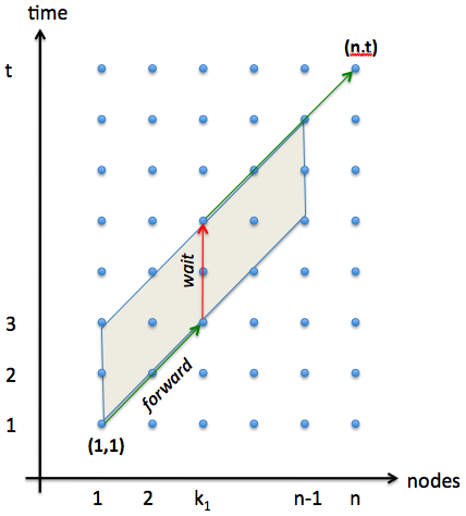
Figure 5: Analyzing the SoA latency in a dynamic random line graph

Figure 5 illustrates the latency under the SoA model. Since each forwarding action to the neighbor costs a time slot, the latency $t-1$ obeys $t-1\geq n-1$, with the best case scenario being the diagonal green path from $(1,1)$ to $(n,t)$. Hence if we want to compute $P(T=t-1)$, we have to consider all paths that use the diagonal ”forward” segments and vertical ”wait” segments, and are contained in the shaded parallelogram; these segments eventually reach $(n,t)$. The width of this parallelogram is $t-n$.

We borrow the techniques used in the CuT probability computation previously and note that paths with $m$ waiting points are possible inside this parallelogram with $1\leq m\leq\min(n-1,t-n)$. Using similar techniques as the CuT computation, we can compute the probability of a certain path $P$ inside the parallelogram with $m$ waiting points (or “bends”) as follows:

$$Pr\{P\} = \pi_{on}^{n-m-1}\pi_{off}^{m}(1-p)^{t-n-m}p^{m}$$ (12)

Let the number of paths that have exactly $m$ waiting points (or “bends”) be $N_{m}$. Since a path may be generated by independently choosing $m$ bending points each on the diagonal and vertical axes of the parallelogram, $N_{m}={n-1\choose m}{t-n-1\choose m-1}$. Therefore, the latency probability distribution for $p>0,q>0$ is given by:

$$P(T=t-1)$$

$$= \sum_{m=1}^{\min({n-1,t-n})}{n-1\choose m}{t-n-1\choose m-1}\frac{p^{n-1}q^{m}(1-p)^{t-n-m}}{(p+q)^{n-1}}$$

where $t\geq n$. If $p+q=1$, the Markov chain reduces to the independent $ER(n,p,L_{n})$ scenario, and it can be verified that Equation 3.3 reduces to Equation 2. We have also numerically verified that for $p\rightarrow 1,q\rightarrow 1$, $E[T]=\frac{3}{2}(n-1)$, in agreement with Observation 3.4, and that the general case is in agreement with Corollary 3.8.

4 Stacked and Smashed Representations of Temporal Graphlets

Since there is a solid theory of traditional non-temporal graphs, an obvious question to ask is if the study of some temporal properties may be reduced to studying the same property on an equivalent single non-temporal graph. We consider two such representations – the stacked graph (StG) and the smashed graph (SmG). A stacked graph is constructed by drawing directed edges in the direction of time between successive temporal graphlets in a TGS; a smashed graph is a “collapsed” version of the stacked graph. Alternatively, it is union of the TGs. Clearly, an SmG is a “lossy” version. However, it is far more succinct, and therefore it would be interesting to know when, if at all, it will suffice.

The study of such “reducibility” is helpful in that it will allow us to use well-known graph-theoretic algorithms (and code) on the appropriate representation to easily evaluate whether properties such as reachability, connectivity etc. hold.

We note that the “evolving graph” representation proposed in [12] which labels edges with the times at which they are active is equivalent to the stacked graph but an evolving graph not a traditional graph. Hence reducing to an evolving graph does not allow us to easily leverage existing algorithms or code. It is imaginable that a smashed graph (or its $m$-smashed variant defined later) can be used to quickly answer on-line queries for graph properties in massive temporal graphs even though such queries may only be answered approximately. Therefore, it is interesting and worthwhile to compare the complexity vs. accuracy tradeoffs of smashing for various temporal graphs.

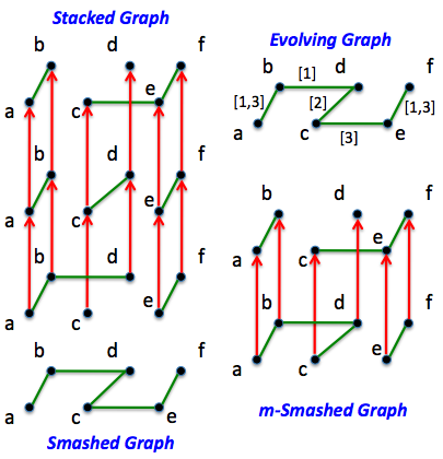
Figure 6: Various representations of temporal graphlets for the TGS in Fig. 1

4.1 Definitions and Basic Properties

We begin with some definitions.

Definition 4.1.

Given a temporal graphlet sequence $G[1,T]$, the stacked graph (StG) of $G[1,T]$ is $StG=(V_{S},E_{S})$, where $V_{S}=\cup_{t}V(t)$, $E_{S}=\cup_{t}E(t)\cup E_{C}$ where $E_{c}$ is a set of “cross edges” connecting vertices of adjacent (in time) graphlets. That is, $E_{c}=\cup_{t,i}(u_{i}(t),u_{i}(t+1))$.

Definition 4.2.

Given a temporal graphlet sequence $G[1,T]$, the smashed graph (SmG) of $G[1,T]$ is $SmG=(V_{M},E_{M})$, where each sequence of $u(t),u(t+1),\ldots$ is replaced by a single vertex $u\in V_{M}$, and $E_{M}=\cup_{t}E(t)$ with endpoints of edges mapped to the replaced vertices in $V_{M}$.

Definition 4.3.

Given a temporal graphlet sequence $G[1,T]$, the $m$-smashed graph (m-SmG) of $G[1,T]$ is $m$-$SmG=(V_{M},E_{M})$, where the smashing operation is not performed on the entire $G[1,T]$ but on each of $G[1,m],G[m+1,2m],G[2m+1,3m],\ldots$ instead.

The various aforementioned representations of the temporal graphlet sequence shown in Figure 1 are illustrated in Figure 6. As mentioned earlier, the StG and Ferreira’s evolving graph model are equivalent in terms of information content. On the contrary SmG is lossy since temporal ordering information is lost during smashing of graphlets. This can result in some false positives (e.g., in the smashed graph, $e\rightarrow b$ is a valid spatio-temporal path, whereas that is not the case in reality).

The technique of $m$-smashing tries to balance the tradeoffs between StG (or evolving graphs) and SmG by restricting the smashing to a smaller number of graphlets at a time. For example, in Figure 6, the first two graphlets are smashed into one, and the result is stacked with the third graphlet. Note that some false positives that were deduced from the SmG (e.g., $e\rightarrow b$ and $e\rightarrow d$) disappear in $m$-SmG. However, some other false positives such as $c\rightarrow b$ still remain.

We note that StG and SmG are non-temporal, or traditional graphs. Consider a property $P$ (definitions of some basic properties studied in this paper are in Table 1). Can the question of whether $P$ is true in $G[1,T]$ be answered by evaluating $P$ on $StG$? If we can, we call such a property stacked-graph reducible (StG-reducible). Similarly, if it can be answered by evaluating $P$ on $SmG$ then we call it smashed-graph reducible (SmG-reducible).

Definition 4.4.

Let $P(H)$ be a function denoting the value (including true/false) of a property P on a structure H where H could be a temporal graphlet sequence or a graph. Then, property $P$ is StG-reducible iff $P(G[1,T]))$ = $P(StG))$, and $P$ is SmG-reducible iff $P(G[1,T]))$ = $P(SmG))$.

Table 1: Examples of temporal graph properties

T-* Property	Definition
T-adjacent$(u,v)$	$\exists(u,v)\in G[1,T]$
T-reachable$(u,v)$	$\exists\{(u,v_{1}),\ldots,(v_{k},v)\}\in G[1,T]$
T-clique	$\max\{X|X\subset V(1),\forall_{u,v}\in X,\textrm{ T-adjacent}(u,v)\}$
T-$k$-connected	$\forall S=\{v_{1},\ldots,v_{k-1}\}\in V_{S}$, if $S$ is removed,
	$\forall_{u,v}$ T-reachable$(u,v)$

We first consider StG-reducibility. We note that some properties such as clique are not “well formed” for directed graphs. In such a case, we admit the use of the undirected version, that is, if $P$ is evaluated on $StG$ by simply ignoring the direction of the edges. We now consider a few properties.

Observation 4.1.

T-reachability is StG-reducible. This is because the cross edges are tantamount to the “store” action.

Observation 4.2.

T-clique is not StG reducible. .

Observation 4.3.

T-$k$-connectivity is StG-reducible if and only if $k$ = 1.

Proof.

That 1-connectivity is StG-reducible follows by repeated application of Observation 4.1. That 2-connectivity is not SG-reducible is illustrated by the “temporal triangle” which is defined as follows: $V(1)=V(2)=V(3)=\{a,b,c\}$, $E(1)=(a,b)$, $E(2)=(b,c)$, $E(3)=(c,a)$. G[T] is 2-connected, but in $G_{S}$ the cross edge between c(1) and c(2) is a bridge. It is easy to see that this is extensible to 3-connectivity in temporal $K_{4}$ and so on. ∎

We now consider Smashed Graphs (SmG) and SmG-reducibility. Since SmG is lossy, it is clear that for the arbitrary case it is not reducible. However, there are two questions: 1) how close can we come? 2) are there special cases when it is reducible? The first question is the subject of later sections, here we state some simple results.

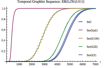
Figure 7: Probability distribution of reachability on a $ER(n,p,L_{n})$ TGS. SmG(all) corresponds to SmG and SmG($m$) correspond to $m$-SmG.

Observation 4.4.

T-clique is SmG-reducible.

Observation 4.5.

T-reachability is SmG-reducible if either of the following holds: (a) there is some G(t=T) that is identical to SmG; (b) there do not exist G(t) and G(t+1) such that the number of connected components increases.

Consider observation 4.5(a) when the identical graphlet either occurs as the first or last in the sequence.

Corollary 4.1.

T-reachability is SmG-reducible if either (a) no edges are ever added; (b) no edges are ever deleted.

Observation 4.5 allows arbitrary additions and deletions, but in a manner that preserves reachability. In practice, these conditions are easily checkable on a sequence of TGs and if they “pass”, we can use the SmG as a way to get the value of graph theoretic properties such as reachability, clique, etc.

The StG- and SmG-reducibility of numerous other graph theoretic concepts is interesting and open.

4.2 Probabilistic Analysis of Smashing

We analyze the properties of stacking and smashing on a random TGS constructed from a sequence of random Erdos-Renyi line graphs given by $\{ER(n,p,L_{n})\}_{t=1}^{T}$.

The probability that a path of latency $t$ time slots (under CuT metric) exists from node $1$ to $n$ is given by Eq. 3. Hence the probability that node $1$ can reach node $n$ within $T=t$ graphlets is given by:

$$P(T<t)=\sum_{\tau=0}^{t-1}{n+\tau-2\choose\tau}(1-p)^{\tau}p^{n-1}$$ (14)

If all the $T$ graphlets are smashed into a single graph, then we can compute the probability of existence of a path from node $1$ to $n$ on the smashed graph SmG. $(j,j+1)\in SmG$ iff $\exists G_{i}\in\{G_{1},G_{2},\ldots,G_{T}\}\>\textrm{s.t.}\>(j,j+1)\in G_{i}$. The probability of this happening is given by:

$$Pr\{(j,j+1)\in SmG\} = 1-Pr\{(j,j+1)\notin SmG\}$$

$$= 1-(1-p)^{t}$$

Therefore, the probability that a path exists within $T$ graphlets is given by the following (since all $n-1$ edge probabilities are independently distributed):

$$P(T_{SmG}<t)=(1-(1-p)^{t})^{n-1}$$ (15)

If we decide to smash $m$ graphlets at a time into one but preserve the rest of the stacked structure, then we have $\frac{T}{m}$ graphlets instead of $T$. The probability of existence of an edge in any of these smashed graphlets is $1-(1-p)^{m}$. Hence the probability distribution of the existence of a path in an $m$-smashed TGS is given by:

$$P(T_{SmG}^{(m)}<t)=\sum_{\tau=0}^{\frac{t}{m}-1}{n+\tau-2\choose\tau}(1-p)^{m\tau}(1-(1-p)^{m})^{n-1}$$ (16)

Figure 7 illustrates the probability distributions of stacked, smashed, and $m$-smashed graphlets. We can observe that while smashed graphs yield only a crude upper bound on the real probabilities (i.e. stacked graphs), the procedure of $m$-smashing is useful since it can yield probability distributions that are much better upper bounds especially for low values of $m$. For graphs where there exist multiple potential paths between source and destination, this process is likely to be even more useful.

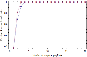
Figure 8: Fraction of reachable node pairs in $MC(n=20,p_{0}=0.005,p=0.5,q=0.05)$ TGS. Squares correspond to SmG and circles to StG

While we have only shown the $ER(n,p,L_{n})$ scenario for the CuT scenario here, it is easy to extend it to the $MC(n,p_{0},p,q,L_{n})$ scenario, since one can apply Eq. 3.3 in this setting to compute the probability of existence of a path within $T=t$ units of time. The probability of existence of an edge in a smashed graphlet in this model can is given by:

$$P(T_{SmG}<t)=(1-\frac{q}{p+q}(1-p)^{t-1})^{n-1}$$ (17)

We omit further details due to paucity of space.

The effect of smashing was also investigated on another derivative metric, namely, the number (or fraction) of reachable pairs over a given time budget $T$ for $G_{u}=K_{n}$. We found by simulations that while the gap between SmG an StG was large for the $ER(n,p)$ scenario (hence motivating $m$-smashing as shown earlier), for the $MC(p_{0},q,p)$ scenario, there were parameter values for which the gap was much lower (as exemplified by Fig. 8). A thorough analysis of the $(q,p)$ parameter space with respect to the reachability metric is a topic of future research.

5 Adaptive Routing in Dynamic Random Graphs

Traditional shortest paths problems attempt to find a path of minimum total distance from $s$ to $t$ and are solved by classical algorithms that satisfy the suboptimal path property [6] (e.g., Dijkstra’s and Bellman-Ford). Shortest paths, routing, and related problems have been considered in various stochastic models (when edges disappear permanently, when they do so periodically, etc.; see [8, 2, 15, 1, 17, 16, 11]) but to the best of our knowledge, have not before been studied in the model considered here. Specifically, we consider the $ER^{t}(n,p,G_{u})$ model with SoA. In the adaptive generalization of the shortest paths concept to temporal graphs (sometimes called “next-hop routing”), the task is to choose, at each routing stage, the best neighbor to route to, if any, in order to minimize the remaining expected travel time. We solve the problem optimally, using a variant of Dijkstra’s algorithm. Because in the adaptive setting we make a routing decision adaptively, each time we arrive at a node, based on its current set of outgoing edges, the algorithm performs its computation going from $t$ to $s$, rather than from $s$ to $t$. To motivate the algorithm, we make the following observations.

Observation 5.1.

In an unweighted graph, an optimal move from a neighbor $v$ of $t$ is to remain at $v$ until the edge $(v,t)$ appears, and then traverse it.

Proof.

Since traversing the edge takes one birth/death time step, the likelihood of being able to traverse edge $(v,t)$ at the next time step is the same as that of being able to traverse $(v^{\prime},t)$ for some mutual neighbor $v^{\prime}$. ∎

Corollary 5.1.

In a weighted graph, an optimal move from $t$’s nearest neighbor $\hat{v}$ will be to remain at $\hat{v}$ until the edge $(\hat{v},t)$ appears.

Observation 5.2.

In an optimal adaptive routing path, there will without loss of generality be no backtracking.

Proof.

Suppose in an optimal solution, we move from node $v$ to $u$. Assume we move only when it gives us a strict improvement, i.e., $METT[u]<METT[v]$. In that case, once at $u$, we will never move to a node with expected remaining travel time greater than $u$’s. ∎

Given this, the optimal deterministic routing algorithm simply moves greedily in order to decrease the remaining minimum expected traversal time ($METT$): at time step, move from the current node $v$ to a neighbor $u\in N(v)$ of minimum $METT(u)$ from $t$, if there is one such that $METT(u)<METT(v)$; otherwise, remain at node $v$ until the next time step. This algorithm assumes an oracle to compute $METT(v)$ for each node $v$, which is done by Algorithm 1.

Algorithm 1 Computing minimum expected traversal times

1:  for each $v$ do

2:     $METT[v]=\infty$

3:  end for

4:  $METT[t]=0$

5:  $Q\leftarrow V$

6:  while $Q\neq\emptyset$ do

7:     $u\leftarrow$ extract-min$(Q)$

8:     for each $v\in N(u)\cap Q$ do

9:        $d_{v}\leftarrow f(p,\{METT[\hat{u}]:\hat{u}\in N(v)-Q\})$

10:        if $d_{v}<METT[v]$ then

11:           $METT[v]=d_{v}$

12:        end if

13:     end for

14:  end while

Let $N(v)$ indicate the neighbors of $v$, and $f(p,S)$ indicate the function computing the $METT$ from a node $v$ to $t$, along a path whose next-hop node is a member of $S$. Given the expected traversal times of the nodes in $S$, $f$ can easily be computed in time $O(|N(v)|\log|N(v)|)$: sort the neighbor nodes $v$ in order of $METT[v]$. The set of neighbor nodes chosen to consider as next-hop candidates in the event that we arrive at node $u$ is the prefix of the $v$ sequence that minimizes the expected remaining traversal time from $v$ to $t$.

Lemma 5.1.

Restricted to an available set of nodes $S$ to use as next hop, and based on the correct $METT$ values of the members of $S$, the function $f(p,S)$ correctly computes $METT[u]$.

Proof.

We need a policy that tells us, when offered a set of the choices, which we should accept, if any, or whether we should instead wait a timestep and try again. Since the graph is Erdos-Renyi, a memoryless policy suffices, i.e., we make the decision based only on the set of available choices, independent of how long we have spent at the current node. Given this, if the cheapest-cost edge is available right now, clearly it should be chosen. If an optimal policy says to take the $k$th cheapest edge (among all the potential choices), if it happens to be the best available, then it follows that we should also take the $j$th cheapest edge, for $1\leq j\leq k$, if it happens to be available. Therefore the only thing to determine then is the best value $k$, i.e., the one leading to the policy that minimizes $METT$ from this node. ∎

Theorem 5.1.

Algorithm 1 correctly computes the $METT$ values for the SoA model.

Proof.

We prove by induction on the nodes removed from $Q$. The expected traversal time of 0 for $t$ is correct by definition. Moreover, by the proof of Corollary 5.1, the expected traversal time of $t$’s nearest neighbor $u$ is $1/p+1$.

Suppose there is at least one node whose computed $METT$ value is incorrect, i.e., larger than optimal. Among such nodes, let $u$ be one whose true $METT$ value is minimum. Note that if $v_{i}$ is removed before $v_{j}$, then $METT[v_{i}]\leq METT[v_{j}]$. This follows from the fact that we remove nodes by performing extract-min operations, and that the function $f(p,\cdot)$ is non-decreasing. There must be at least one path from $u$ to $t$, i.e., $u$ must have at least one neighbor whose true optimal expected time to $t$ is strictly less than $u$’s. In fact, $u$ may have several such neighbors. Call them $v_{1},...,v_{\ell}$. If the true $METT$ values of $v_{1},...,v_{\ell}$ are all smaller than $u$’s. then by the induction assumption their $METT$ values are correct, and hence so is $u$’s.

Now suppose some such $v_{i}$ has not yet been removed. This implies that its computed $METT$ value will be at least $u$’s, even though $v_{i}$’s true $METT$ value is smaller than $u$’s, which contradicts the induction hypothesis. ∎

We can now redefine the CuT model as the one in which all edge weights are 0. The effect of this is that $v$ neighbor set $N(v)$ is replaced in the routing algorithm with the set of all nodes reachable from $v$, since upon arrival at $u$, we can consider cutting through instantly to any node that 1) would be an improvement over $u$ and 2) to which there currently is an accessible path from $u$.

Corollary 5.2.

Modified appropriately, Algorithm 1 correctly computes the optimal traversal times for the CuT model, as well as for the nonnegative integer-weighted model subsuming SoA and CuT.

Proof.

An oracle to compute the probability that there exists an edge between $v$ and $u$, for all pairs $(v,u)$ can be computed in polynomial time by dynamic programming. We omit the details due to lack of space. ∎

6 Discussion and Future Work

This paper marks the first step toward a research program aimed at developing a theory of temporal graphs from both stochastic and deterministic (or classical) points of view. We plan to develop the research program in multiple directions. First, the probability distribution results in Sec. 3 need to be extended beyond simple scenarios such as dynamic random path, especially to scenarios where there are multiple possible (intermittent) paths between the source and the destination. Second, in addition to the T-* properties discussed in Sec. 4 other properties such as chromatic number, independent set, and dominating set are worth investigating. One interesting question is whether $m$-smashing can be improved by a non-uniform choice of $m$. If the deterministic sequence of graphs is known, then this is akin to a compression problem where more graphlets will be smashed around times when the temporal ordering does not matter much, and less graphlets will be smashed around other times, thus preserving the temporal structure. However, for a given dynamic random graph model, it may be interesting to develop rules of thumb for non-uniform smashing. In addition to graphlet union (or SmG), graphlet intersection can be interesting since it can be used to quantify redundancy in spatio-temporal paths in a TGS.

References

- [1] Aruna Balasubramanian, Brian Neil Levine, and Arun Venkataramani. Dtn routing as a resource allocation problem. In SIGCOMM, pages 373–384, 2007.
- [2] Amotz Bar-Noy and Baruch Schieber. The canadian traveller problem. In SODA, pages 261–270, 1991.
- [3] Prithwish Basu and Chi-Kin Chau. Opportunistic forwarding in wireless networks with duty cycling. In Proc. of ACM MobiCom Workshop on Challenged Networks (CHANTS), September 2008.
- [4] Prithwish Basu and Saikat Guha. Effect of limited topology knowledge on opportunistic forwarding in ad hoc wireless networks. In Proc. WiOpt), Avignon, France, June 2010.
- [5] H. Baumann, P. Crescenzi, and P. Fraigniaud. Parsimonious flooding in dynamic graphs. In Proc. of ACM Symposium on Principles of Distributed Computing (PODC), Calgary, Alberta, Canada, August 2009.
- [6] Dimitri P. Bertsekas. Data Networks. Prentice Hall, 2nd edition, 1992.
- [7] Chi-Kin Chau and Prithwish Basu. Exact analysis of latency of stateless opportunistic forwarding. In Proc. of IEEE INFOCOM, Rio de Janeiro, Brazil, April 2009.
- [8] Shuchi Chawla and Tim Roughgarden. Single-source stochastic routing. In APPROX-RANDOM, pages 82–94, 2006.
- [9] A. E. F. Clementi, C. Macci, A. Monti, F. Pasquale, and R. Silvestri. Flooding time in edge-markovian dynamic graphs. In Proc. of ACM Symposium on Principles of Distributed Computing (PODC), Toronto, Canada, August 2008.
- [10] A. E. F. Clementi, A. Monti, F. Pasquale, and R. Silvestri. Communication in dynamic radio networks. In Proc. of ACM Symposium on Principles of Distributed Computing (PODC), Portland, OR, August 2007.
- [11] Camil Demetrescu and Giuseppe F. Italiano. Experimental analysis of dynamic all pairs shortest path algorithms. ACM Transactions on Algorithms, 2(4):578–601, 2006.
- [12] A. Ferreira. Building a reference combinatorial model for manets. IEEE Network, 18(5):24–29, 2004.
- [13] Geoffrey Grimmett. Percolation. Springer, 1999.
- [14] Pan Hui, Augustin Chaintreau, Richard Gass, James Scott, Jon Crowcroft, and Christophe Diot. Pocket switched networking: Challenges, feasibility, and implementation issues. In Proc. of Workshop on Autonomic Communication (WAC), Greece, October 2005.
- [15] Sushant Jain, Kevin Fall, and Rabin Patra. Routing in a delay tolerant network. In SIGCOMM ’04: Proceedings of the 2004 conference on Applications, technologies, architectures, and protocols for computer communications, pages 145–158, New York, NY, USA, 2004. ACM.
- [16] Goran Konjevod, Soohyun Oh, and Andréa W. Richa. Finding most sustainable paths in networks with time-dependent edge reliabilities. In LATIN, pages 435–450, 2002.
- [17] Shouwen Lai and Binoy Ravindran. On distributed time-dependent shortest paths over duty-cycled wireless sensor networks. In INFOCOM, pages 1685–1693, 2010.
- [18] Shashi Merugu, Mostafa Ammar, and Ellen Zegura. Space-time routing in wireless networks with predictable mobility. Technical Report GIT-CC-04-07, Georgia Institute of Technology, College of Computing, March 2004.
- [19] Peter J. Mucha, Thomas Richardson, Kevin Macon, Mason A. Porter, and Jukka-Pekka Onnela. Community structure in time-dependent, multiscale, and multiplex networks. Science, 328(5980):876–878, 2010.
- [20] Ram Ramanathan. Challenges: A radically new architecture for next generation mobile ad hoc networks. In Proc. of ACM MobiCom, Cologne, Germany, August 2005.
- [21] J. Tang, M. Musolesi, C. Mascolo, and V. Latora. Temporal distance metrics for social network analysis. In Proc. ACM SIGCOMM Workshop on Online Social Networks (WOSN), Barcelona, Spain, August 2009.