$(\alpha,\beta)$ Fibonacci Search

Abstract

Knuth [12, Page 417] states that “the (program of the) Fibonaccian search technique looks very mysterious at first glance” and that “it seems to work by magic”. In this work, we show that there is even more magic in Fibonaccian (or else Fibonacci) search. We present a generalized Fibonacci procedure that follows perfectly the implicit optimal decision tree for search problems where the cost of each comparison depends on its outcome.

1 Introduction

Binary search is the most common algorithm for comparison-based search in sorted arrays in which random access is permitted. The worst-case complexity is logarithmic on the length $n$ of the sequence. A general information-theoretic lower bound based on decision trees shows that any comparison-based search algorithm needs in the worst-case at least logarithmic steps to locate an item in a sorted array.

In the analysis of binary search, the cost of each comparison step is usually some fixed constant. However, there are natural problems where the cost of a comparison depends on its outcome. For example, during the search an overestimation of the unknown value may cost more than an underestimation or the opposite. An interesting example is provided by TCP (Transmission Control Protocol) flows that transmit data over the Internet. Each TCP flow has a parameter called the congestion window, which is used to regulate its transmission rate. A small congestion window will cause the flow to use less than the available bandwidth whereas a large congestion window will cause delays and packet losses in case of overflows. Most TCP flows use the AIMD (Additive Increase Multiplicative Decrease) algorithm to adjust their congestion window to the current network conditions [11, 6]. The cost induced to a TCP flow for underestimating the optimal congestion window differs from the cost of overestimating it.

We consider the following toy-example of asymmetric cost binary search. Assume that we want to experimentally estimate the minimum speed at which the airbags of a particular car will deploy. Assuming that all other parameters of the experiment are held constant (ceteris paribus assumption), we want to identify the minimum speed with one decimal digit precision, at which the airbags deploy. We are given the information that the requested minimum speed is in the closed interval 10-20 km/h (interval of uncertainty). Finally, there is asymmetry in the cost of each comparison (crash test). The damage caused by a crash test in the interval of uncertainty is 500€ if the airbags do not deploy and 1500€ if the airbags open. What is the minimum worst-case cost to identify the requested speed? The solution of this example is given in Section 7. A similar example is the leaky shower problem described in [10].

An amusing example of a closely related search problem is given in the lecture notes of [15]. Given two absolutely identical eggs, how many times do we have to drop an egg to identify how strong the eggs are? In this problem, the unknown value has to be found with at most two overestimates. The cracking eggs problem is an example of asymmetric cost binary search where there is a fixed bound on the number of the outcomes of one type, usually the overestimates. Binary search with a bounded number of overestimates is discussed in [3, 16], where it is shown that it is related to binomial trees.

In this work, we consider the problem of searching in a sorted array when the cost of each comparison depends on its outcome. For example, in the binary case, each comparison with outcome “$\leq$” has a fixed cost $\alpha$ and each comparison with outcome “$>$” a fixed cost $\beta$. We assume that $\alpha$ and $\beta$ are integers or rational multiples of each other, such that $\alpha\geq 1$ and $\beta\geq 1$. We then generalize the results to the case of searching with more than two outcomes. A problem related to the (binary) search procedure is the construction of (binary) search trees. An $O(n)$ time algorithm to construct a binary search tree for $(\alpha,\beta)$ binary search is presented in [5]. The results of [5] are based on an interesting relation of the search tree structure to the Pascal’s triangle and are valid for any positive numbers $\beta\geq\alpha>0$. The case of $(1,2)$ binary search trees is further discussed in [14] where the relation of the $(1,2)$ binary search problem to the original Fibonacci sequence is identified. Binary trees with choosable edge lengths are discussed in [13]. A general treatment of binary search with asymmetric costs is given in [10]. The costs of binary search in [10] can be real numbers, but the search procedure proposed is only near optimal. The same problem is studied in [9] with tools from dynamic programming. Tree structures for searching with asymmetric costs when the number of outcomes of each comparison may be larger than two is discussed in [4] where optimal lopsided trees are analyzed.

The focus of this work is on a lightweight search algorithm for asymmetric cost search and not on the explicit construction of the corresponding search tree. As such, the main contribution of this work is an optimal lightweight search procedure for $(\alpha,\beta)$ binary search without the explicit construction of the binary search tree. Furthermore, we show that the results of this work are valid for search trees of higher degrees. The generalization of the Fibonacci sequences used in this work seems to naturally fit the search problem and gives simple, optimal results. Even though the problem has been studied in the past, no algorithm that is both optimal with respect to its running time and the cost of the generated solution has been presented.

Interestingly, there is an early search algorithm called Fibonacci search or Fibonaccian search [7, 12], which uses the classic Fibonacci sequence to lead the item selection procedure in the sorted array. Fibonacci search is a variation of binary search that avoids the division operations required in binary search to select the middle item. At that early days of computer science a division by two or even a simple shift operation could be an undesirably expensive operation for a computer program.

Knuth [12, Page 417] states that “the (program of the) Fibonaccian search technique looks very mysterious at first glance” and that “it seems to work by magic”. In this work, we show that there is even more magic in Fibonaccian (or else Fibonacci) search. The generalized Fibonacci procedure of this work follows perfectly the implicit optimal decision tree for search problems where the cost of each comparison depends on its outcome.

Contribution. We present $(\alpha,\beta)$ Fibonacci search, an optimal lightweight search procedure for searching with asymmetric costs. The algorithm is simple and intuitive and the first, to our knowledge, optimal algorithm for a classic problem when the comparison costs are fixed integers or rationally multiples of each other. We define Fibonacci decision trees and use them to prove the information theoretic lower bounds of the search problem. Even though this structure exists implicitly in more general works like [4], its significance for search and decision problems has not been sufficiently stressed so far. Moreover, we present and solve an interesting guessing game with $h$ outcomes per comparison and discuss applications of it in prefix codes. Finally, we present an abstract class definition and an implementation of the search algorithm.

The rest of this work is organized as follows: The asymmetric cost search problem is defined in Section 2. In Section 3, Fibonacci-like sequences are defined. The lower bound on the worst-case cost is presented in Section 4. The $(\alpha,\beta)$ Fibonacci search algorithm is described in Section 5. Applications of $(\alpha,\beta)$ Fibonacci search are presented in Section 6 and a final discussion is given in Section 7.

2 $(\alpha,\beta)$ Binary Search

The formal definition of the asymmetric binary search problem follows.

Definition 1

The $(\alpha,\beta)$ binary search problem. An array $V$ of $n$ items sorted in increasing order is given. Each item of the array can be accessed in time $O(1)$. For any value $x$ and any item $v_{k}$ of $V$ the cost of the comparison $x\leq v_{k}$ is

$\mbox{cost of }(x\leq v_{k})=\left\{\begin{array}[]{ll}\alpha,\;\mbox{ if the outcome if true, }\\ \beta,\;\mbox{ if the outcome is false. }\end{array}\right.$

Parameters $\alpha$ and $\beta$ are strictly positive integers. The cost of a search is equal to the sum of the costs of all comparison operations $x\leq v_{k}$ performed during the search.

We assume that the searched item $x$ is in the array $V.$ The results of this work can be extended to searches for items that may not belong to $V$ by comparing at the end of the search the requested item with the item found.

Cost and complexity. The cost metric in the search procedure can be used to model diverse criteria. For example in [14] the cost corresponds to computational complexity; underestimation costs one processor operation and overestimation two processor operations. The cost can also correspond to other metrics like the budget in the airbags example or some efficiency criterion in the TCP flow example.

3 Sequences

In the analysis of the lower bound and the search algorithm for the $(\alpha,\beta)$ search problem we will use a generalization of Fibonacci sequences. In this Section we provide the necessary definitions of the sequences that we will use. We start with the well-known Fibonacci sequence.

Definition 2

The Fibonacci sequence is given by the recurrence relation

$$f(k)=f(k-1)+f(k-2)\quad,$$ (1)

with initial values $f(k)=0$, for $k\leq 0$, and $f(1)=1$.

We define the following generalization of the Fibonacci sequence where each term is the sum of two preceding terms, which however may not be the immediately preceding terms.

Definition 3

The $(\alpha,\beta)$ Fibonacci sequence. Given integers $\alpha\geq 1$ and $\beta\geq 1$, the $(\alpha,\beta)$ Fibonacci sequence is given by the recurrence relation

$$g(k)=g(k-\alpha)+g(k-\beta)\quad,$$ (2)

with initial values, unless otherwise specified, $g(k)=0$, for $k<0$, and $g(0)=1$.

The $(\alpha,\beta)$ Fibonacci sequence is actually a family of generalized Fibonacci sequences. Some well known sequences that are related to members of the $(\alpha,\beta)$ Fibonacci family are:

• The classic Fibonacci sequence for $\{\alpha,\beta\}=\{1,2\}$ and initial values $f(0)=0$ and $f(1)=1$.

• The Padovan sequence and the Perrin sequence for $\{\alpha,\beta\}=\{2,3\}$ and initial values $f(0)=f(1)=f(2)=1$ and $f(0)=3,f(1)=0,f(2)=2$, respectively.

Given the parameters $\alpha$ and $\beta$ of an $(\alpha,\beta)$ Fibonacci sequence, let

$$\ell=\min\{\alpha,\beta\}\mbox{ and }u=\max\{\alpha,\beta\}\quad.$$ (3)

In the analysis of the $(\alpha,\beta)$ binary search problem we will encounter the following sequence, in which the term $k$ of the sequence is equal to the sum of the last $\ell$ terms of the corresponding $(\alpha,\beta)$ Fibonacci sequence.

Definition 4

Given integers $\alpha\geq 1$ and $\beta\geq 1$, let $\ell=\min\{\alpha,\beta\}$. Then let

$$G(k)=\sum_{i=1}^{\ell}g(k+1-i)\quad,$$ (4)

where $g(k)$ is the $(\alpha,\beta)$ Fibonacci sequence.

It turns out that the $G(k)$ sequence is also an $(\alpha,\beta)$ Fibonacci sequence but with its own initial values.

Proposition 1

$G(k)$ is an $(\alpha,\beta)$ Fibonacci sequence.

Proof

$$G(k)=\sum_{i=1}^{\ell}g(k-i+1)=\sum_{i=1}^{\ell}g(k-i+1-\alpha)+\sum_{i=1}^{\ell}g(k-i+1-\beta)$$

$$\Rightarrow G(k)=G(k-\alpha)+G(k-\beta)\quad.$$

The appropriate initial values for $G(k)$ are $G(k)=0$ for $k<0$ and $G(k)=1$ for $0\leq k<u$.

Note that if $\ell=1$ then, as expected, the sequences $G(k)$ and $g(k)$ coincide (for the same parameters $\alpha$ and $\beta$).

Closed form expressions are known for example for the terms of the classic Fibonacci sequence, the Padovan sequence and the Perrin sequence. Since every member of the $(\alpha,\beta)$ Fibonacci sequences is defined by a linear recurrence, there exists a closed-form solution for each sequence. However, we are not aware of a general closed form expression for the complete $(\alpha,\beta)$ Fibonacci family. Closed form estimations of terms of generalized Fibonacci sequences are given for example in [4, 19, 9, 10]. The following Proposition follows directly from Lemma 1 of [9] and provides upper and lower bounds on the terms of the $G(k)$ Fibonacci sequence.

Proposition 2

For strictly positive integers $\alpha$ and $\beta$ it holds

$$2^{\frac{k+1-u}{u}}\leq G(k)\leq 2^{\frac{k+2-u}{\ell}}\quad.$$ (5)

4 The Lower Bound

We present an information-theoretic lower bound on the worst-case cost of the $(\alpha,\beta)$ binary search problem. Like the known lower bounds for binary search, the approach is based on decision trees. To handle the asymmetry of the comparison costs we define a special type of decision tree.

Definition 5

The $(\alpha,\beta)$ decision tree. The root node of the tree has level $0$. Let $v$ be a node at level $d_{v}$ of the tree. Then
$\mbox{ node }v\left\{\begin{array}[]{ll}\mbox{ is either a leaf of the tree, }\\ \mbox{ or it has a left child at level $(d_{v}+\alpha)$ and a right child at level $(d_{v}+\beta)$. }\end{array}\right.$

Note that the term level is used to represent the weighted depth of the tree nodes. Each level of the tree corresponds to a particular cost value.

Definition 6

The level of an $(\alpha,\beta)$ decision tree is the maximum level of any of its nodes. The depth of a node is the common depth of tree nodes, i.e., the number of links from the root to the node. The depth of an $(\alpha,\beta)$ decision tree is the maximum depth of any of its nodes.

The distinguishing property of $(\alpha,\beta)$ decision trees is that nodes which have the same parent may be located at different tree levels. The general form of an $(\alpha,\beta)$ decision tree is shown in Figure 1a. Two instances of $(\alpha,\beta)$ decision trees are presented in Figure 2.

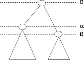
(a) An $(\alpha,\beta)$ decision tree.

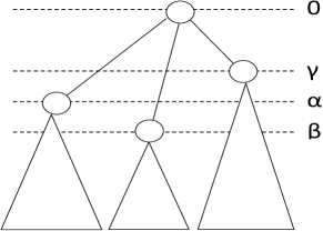
(b) An h-decision tree for h=3.

Figure 1: Two instances of asymmetric cost decision trees.

Proposition 3

The number of nodes at level $k$ of a complete $(\alpha,\beta)$ decision tree is the value of term $g(k)$ of corresponding $(\alpha,\beta)$ Fibonacci sequence of Equation 3.

Proof

The number of nodes at level $k$ is equal to the sum of the number of nodes at levels $(k-\alpha)$ and $(k-\beta)$. Furthermore, there is one node at level $0$, the root node.

Proposition 4

The number of leaf nodes of a complete $(\alpha,\beta)$ decision tree of level $k$ is $G(k)$, where $G(k)$ is the $(\alpha,\beta)$ Fibonacci sequence of Equation 4.

Proof

The nodes of level $k$ are of course leaf nodes of the tree. Additionally, any node with level in $(k-1),(k-2),\dots,(k+1-\ell)$ must also be a leaf node since the node cannot have any descendants with level at most $k$.

Proposition 5

The wort-case cost for an $(\alpha,\beta)$ binary search problem with $n$ items is at least $k$, where $k$ is the minimum index such that $G(k)\geq n$.

Proof

Any search procedure for an $(\alpha,\beta)$ binary search problem can be represented with a corresponding $(\alpha,\beta)$ decision tree. The level of the decision tree corresponds to the worst-case cost of the respective search procedure. From Proposition 4 we know that any $(\alpha,\beta)$ decision tree with level up to $k-1$ can have at most $G(k-1)$ leaves. Hence any search procedure will have worst-case cost at least $k$, where $k$ is such that $G(k)\geq n$.

5 $(\alpha,\beta)$ Fibonacci Search

We propose $(\alpha,\beta)$ Fibonacci search, an algorithm for the $(\alpha,\beta)$ binary search problem. The proposed algorithm is a dichotomic search algorithm like binary search but uses the $G(k)$ sequence numbers to dichotomize the item sets and to select the items to be examined. The algorithm is a generalization of Fibonacci search [7] to $(\alpha,\beta)$ Fibonacci sequences.

5.1 The Algorithm (short version)

Algorithm $(\alpha,\beta)$ Fibonacci search

Input:

A sorted array $V$ with $n$ items and a requested item $x$ in $V$. The items in V are indexed from $0$ to $n-1$.

Step 0:

$(\alpha,\beta)$ Fibonacci numbers. Prepare the $(\alpha,\beta)$ Fibonacci numbers up to index $k$ such that $G(k)\geq n$.

Step 1:

Initializations. Let $z=k-\alpha$, $left=0$, $right=n-1$.

Step 2:

Search Loop.
While $(left<right)$

1. $index=left+G(z);$ if $(index>right)$ then $\{index=right\};$

2. $value=v[index]$

3. Compare $(x\leq value)$

   true:

   $right=index;z=z-\alpha;$

   false:

   $left=index+1;z=z-\beta;$

Step 3:

Check if $(V[index]==x).$ This step is only necessary if the requested item x may not belong to V.

First the algorithm prepares the sequence of $G(k)$ numbers up to the first term $G(k)$ of the sequence such that $G(k)\geq n$. Then, the algorithm enters the search loop. In each round, the algorithm selects either the left subtree or the right subtree of the implicit $(\alpha,\beta)$ decision tree. If the current subtree has $G(z)$ leaves then the number of leaves of the left tree is $G(z-\alpha)$ and of the right subtree $G(z-\beta)$. If the current subtree has less than $G(z)$ leaves (if $n$ is not an $(\alpha,\beta)$ Fibonacci number), then the right subtree will also have less than $G(z-\beta)$ leaves.

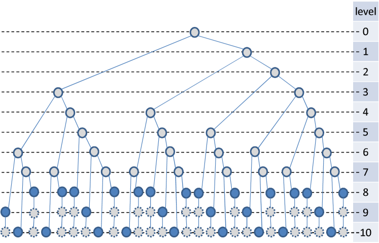
(a) The complete $(3,1)$ decision tree with level 10. The maximum number of leaves of a $(3,1)$ decision tree with level 10 is equal to the number of nodes at level 10 of the depicted tree.

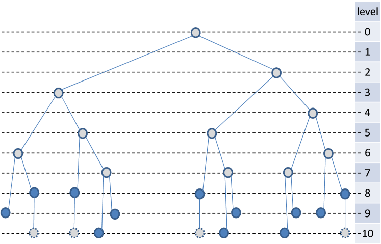
(b) The complete $(3,2)$ decision tree with level 10. The maximum number of leaves of a $(3,2)$ decision tree with level 10 is equal to the number of nodes at levels 9 and 10 of the depicted tree.

Figure 2: Two instances of $(\alpha,\beta)$ Fibonacci trees with level 10. The dark nodes are the nodes at which the $(\alpha,\beta)$ Fibonacci search algorithm terminates.

5.2 Complexity and Cost

From the description of the $(\alpha,\beta)$ Fibonacci search algorithm and the lower bound of Section 4, it follows that the worst-case cost of the algorithm is optimal.

Proposition 6

The worst-case cost of the $(\alpha,\beta)$ Fibonacci search algorithm for the $(\alpha,\beta)$ binary search problem is optimal.

Proof

The decision tree of the search algorithm is the $(\alpha,\beta)$ decision tree used in the proof of the lower bound in Section 4. Hence, the worst-case performance matches the lower bound.

We will show that the computational complexity of the $(\alpha,\beta)$ Fibonacci search algorithm is logarithmic on the number $n$ of the items.

Proposition 7

Given an $(\alpha,\beta)$ binary search problem, the level of the implicit $(\alpha,\beta)$ decision tree of algorithm $(\alpha,\beta)$ Fibonacci search is at most $u\cdot\lceil\log_{2}n\rceil$.

Proof

(Sketch.) Recall that $u=\max\{\alpha,\beta\}$. The worst-case complexity of binary search for the $(\alpha,\beta)$ binary search problem is $\lceil\log_{2}n\rceil=O(\log n)$. Hence, the worst-case cost of binary search is at most $u\cdot\lceil\log_{2}n\rceil$. The worst-case cost of $(\alpha,\beta)$ Fibonacci search is optimal and thus not larger that $u\cdot\lceil\log_{2}n\rceil$.

Corollary 1

The depth of the $(\alpha,\beta)$ decision tree is not larger than $\lceil u/\ell\rceil\lceil\log_{2}n\rceil$.

Proof

Follows from Proposition 7 since every round of the search procedure increases the level (cost) of the search by at least $\ell$. A slightly weaker result follows from Proposition 2.

Proposition 8

The complexity of the $(\alpha,\beta)$ Fibonacci search algorithm is at most logarithmic on the number of items $n$.

Proof

The algorithm first prepares the $(\alpha,\beta)$ Fibonacci sequence up to the first $k$, such that $G(k)\geq n$. From Proposition 7, the level of the corresponding decision tree is bounded by $u\cdot\lceil\log_{2}n\rceil$, and, thus, by $O(\log n)$, assuming $u$ is a constant. From Corollary 1 we obtain that $k\leq\lceil u/\ell\rceil\cdot\lceil\log_{2}n\rceil=O(\log n)$. The main phase of the algorithm is the search loop. The loop is executed not more than $\lceil u/\ell\rceil\cdot\lceil\log_{2}n\rceil$ times, since in each loop the depth of the remaining tree is reduced by at least one. Thus, the overall complexity is $O(\lceil u/\ell\rceil\cdot\lceil\log_{2}n\rceil)=O(\log n)$. Note that a factor $u$ is hidden in the preparation time of the algorithm (calculation of the terms of $G(k)$) and a factor $u/\ell$ in the complexity of each item search.

5.3 The Algorithm (full version)

We present now the full version of the $(\alpha,\beta)$ Fibonacci search algorithm which is also average-case optimal, assuming that all items of the population are equiprobable. When $n=|V|$ is an $(\alpha,\beta)$ Fibonacci number, then the lowest layer of the corresponding search tree is complete and the short version of Section 5.1 is optimal in the average case too. If, however, $n$ is not an $(\alpha,\beta)$ Fibonacci number, then some nodes of the lowest layer of the complete search tree are not used. To make the search optimal in the average case, the surplus nodes have to be assigned to highest cost nodes of the search tree. Let $k$ be the level of the corresponding search tree. Then the number of surplus nodes cannot exceed $g(k)$ because else the lowest of the tree could be avoided. We assume that all surplus nodes are assigned to the lowest layer from right to left. The full version of $(\alpha,\beta)$ Fibonacci search traverses the implicit decision tree down to the corresponding leaf. During its descendance, it simply keeps track how many surplus nodes correspond to its current subtree. The code of the algorithm becomes a little more involved, but its asymptotic complexity remains the same. Due to lack space, we omit the detailed description of the algorithm.

6 Applications

Fibonacci sequences can be generalized to sequences of higher order. For example, the common Fibonacci sequence of order three is the Tribonacci sequence. Further members in increasing order are the Tetranacci, Pentanacci and Hexanacci sequences [18]. Since $(\alpha,\beta)$ Fibonacci search fits perfectly the decision tree of the $(\alpha,\beta)$ binary search problem we are tempted to examine what happens if we turn to higher order Fibonacci sequences.

6.1 A Guessing Game

The generalization of the asymmetric cost binary search problem to searching with more outcomes per comparison gives the following guessing game.

Definition 7

The h-outcomes guessing game. An array $V$ with $n$ items sorted in increasing order and access time $O(1)$ for each item, is given. To search in an interval I, the following comparison operation is supported: The interval I has to be partitioned into a partition P of h consecutive intervals defined with h-1 values $v_{1}\leq v_{2}\leq\dots\leq v_{h-1}$. For any value $x$ and any partition P, the cost of finding in which of the intervals of P item $x$ belongs, is

$\mbox{cost of (in which interval of P is x)}=w_{i},\mbox{ if the searched item is in interval i, for }i=0,1,\dots,h-1,$

where the weights or costs $w_{i}$, for $i=0,1,\dots,h-1$, are strictly positive integers. The cost of a search is equal to the sum of the costs of all comparison operations performed during the search. As in the binary search case, the requested item $x$ is assumed to belong to the array $V,$ else the requested item has to be compared at the end of the search with the item found.

The results of Section 4 on the lower bound of the two outcomes $(\alpha,\beta)$ binary search can be extended to obtain h-decision trees this search problem with $h$ outcomes. Similarly, it is straightforward to generalize the $(\alpha,\beta)$ Fibonacci search algorithm of Section 5 to the h-Fibonacci search algorithm that optimally solves the h-outcomes search problem. Due to lack space, we omit the detailed description and proofs of these results.

6.2 Coding with Unequal Letter Costs

The problem of searching with asymmetric costs is strongly related to optimal prefix codes [17, 8]. The encoding of letters that may have different lengths but occur with the same probability is known as the Varn coding problem and can be solved in polynomial time.

The results of this work, provide simple strict lower bounds on the worst-case cost of Varn codes with lengths that are integers or rational multiples of each other. In particular, an implicit description of an optimal Varn encoding or an optimal Varn encoding with the alphabetic property (the additional constraint that the encoding of the words must preserve their alphabetical order) can be calculated in logarithmic time. The h-Fibonacci decision tree provides a tight lower bound on the worst case cost for the encoded form and the h-Fibonacci search algorithm gives an optimal coding of the letters that matches the lower bound. Then, the encoding of any particular word can also be calculated in logarithmic time. This might be useful if the domain (the item set to be encoded) is very large, for example exponential on some problem parameter. In this case we may generate an implicit encoding, given any specific (possibly implicit) ordering of all words and then generate only the words that are actually used.

7 Discussion

We consider the $(\alpha,\beta)$ Fibonacci search algorithm and its generalization, the h-Fibonacci search algorithm, fundamental tools that can be used within the solutions of other computational problems. For this reason, we developed a prototype implementation of the two algorithms within a standard Java class library that can be found at [1].

Back to the airbag example of Section 1, the interval of uncertainty contains $101$ distinct values $(10.0,10.1,\dots,20.0)$. We use the implemented $(\alpha,\beta)$ Fibonacci search algorithm with $\alpha=1$ and $\beta=3$ to find that the level of the corresponding $(\alpha,\beta)$ decision tree is $14$ (since G(13) = 88 and G(14) = 129, for $\alpha=1$ and $\beta=3$). Thus, the worst-case cost is $500\cdot 14=$ 7000€. The corresponding tree generated by normal binary search has worst-case depth $\lceil\log_{2}101\rceil=7$ and thus, the cost of the binary search solution can be up to $7\cdot 1500=$10500€. Since the lowest layer of the binary search tree is not complete, this cost can be reduced to $6\cdot 1500+1\cdot 500=$ 9500€ by using the $101$ leftmost leaves (because in this case the right branches have the higher cost).

The difference between the costs $7000$ and $9500$, albeit not colossal, is without doubt significant. Preliminary experiments indicate the, rather expected, result, that the benefits of using $(\alpha,\beta)$ Fibonacci search increase as the ratio $u/\ell$ increases. The experiments also indicate that the benefits in the average case cost of the search problem if $(\alpha,\beta)$ Fibonacci search is used, are still significant, albeit smaller than with the worst-case criterion.

A further interesting question is if the results of this work can be generalized to support real positives $\alpha$ and $\beta$, possibly with the use of the Pascal’s triangle like in [5] or techniques from [4].

References

-
[1]
abFib.
A Java class implementation for Fibonacci
search, 2010.
http://utopia.duth.gr/pefraimi/projects/abFib/. - [2] Mordecai Avriel. Nonlinear Programming: Analysis and Methods. Dover Publications, September 2003.
- [3] Jon Louis Bentley and Donna J. Brown. A general class of resource tradeoffs. Journal of Computer and System Sciences, 25(2):214 – 238, 1982.
- [4] Vicky Siu-Ngan Choi and Mordecai J. Golin. Lopsided trees, i: Analyses. Algorithmica, 31(3):240–290, 2001.
- [5] David M. Choy and C. K. Wong. Bounds for optimal binary trees. BIT Numerical Mathematics, 17:1–15, 1977.
- [6] P.S. Efraimidis and L. Tsavlidis. Window-games between TCP flows. In Lecture Notes in Computer Science (SAGT 2008), volume 4997, pages 95–108, Springer-Verlag Berlin Heidelberg, 2008.
- [7] David E. Ferguson. Fibonaccian searching. Commun. ACM, 3(12):648, 1960.
- [8] Mordecai J. Golin, Claire Kenyon, and Neal E. Young. Huffman coding with unequal letter costs. In STOC ’02: Proceedings of the thiry-fourth annual ACM symposium on Theory of computing, pages 785–791, New York, NY, USA, 2002. ACM.
- [9] K. Hinderer. On dichotomous search with direction-dependent costs for a uniformly hidden object. Optimization, 21:215–229, 1990.
- [10] Sanjiv Kapoor and Edward M. Reingold. Optimum lopsided binary trees. J. ACM, 36(3):573–590, 1989.
- [11] R. Karp, E. Koutsoupias, C. Papadimitriou, and S. Shenker. Optimization problems in congestion control. In Proceedings of FOCS ’00, page 66, Washington, DC, USA, 2000. IEEE Computer Society.
- [12] D.E. Knuth. The Art of Computer Programming, volume 2 : Seminumerical Algorithms. Addison-Wesley Publishing Company, second edition, 1981.
- [13] Jens Maßberg and Dieter Rautenbach. Binary trees with choosable edge lengths. Inf. Process. Lett., 109(18):1087–1092, 2009.
- [14] Thomas Ottmann, Arnold L. Rosenberg, Hans-Werner Six, and Derick Wood. Binary search trees with binary comparison cost. International Journal of Parallel Programming, 13(2):77–101, 1984.
-
[15]
Satish Rao.
Cracking eggs (or asymmetric cost binary search).
CS270 Lecture Notes, Lecture 25, 2001.
http://citeseerx.ist.psu.edu/viewdoc/summary?doi=10.1.1.23.72. - [16] J. van Leeuwen, N. Santoro, J. Urrutia, and S. Zaks. Guessing games and distributed computations in synchronous networks. In 14th International Colloquium on Automata, languages and programming, pages 347–356, London, UK, 1987. Springer-Verlag.
- [17] Ben Varn. Optimal variable length codes (arbitrary symbol cost and equal code word probability). Information and Control, 19(4):289 – 301, 1971.
- [18] Wikipedia. Generalizations of fibonacci numbers — Wikipedia, the free encyclopedia, 2010. [Online; accessed 26-Febrouary-2010].
- [19] D.A. Wolfram. Solving generalized fibonacci recurrences. The Fibonacci Quarterly, 36(2):129–145, 1998.