Robust Estimation of Operational Risk

According to the Loss Distribution Approach, the operational risk of a bank is determined as the $99.9\%$ quantile of the respective loss distribution, covering unexpected severe events. The $99.9\%$ quantile can be considered a tail event. As supported by the Pickands-Balkema-de Haan Theorem, tail events exceeding some high threshold are usually modeled by a Generalized Pareto Distribution (GPD). Estimation of GPD tail quantiles is not a trivial task, in particular if one takes into account the heavy tails of this distribution, the possibility of singular outliers, and, moreover, the fact that data is usually pooled among several sources.
In such situations, robust methods may provide stable estimates when classical methods already fail.
In this paper, optimally-robust procedures MBRE, OMSE, RMXE are introduced to the application domain of operational risk. We apply these procedures to parameter estimation of a GPD at data from Algorithmics Inc. To better understand these results, we provide supportive diagnostic plots adjusted for this context: influence plots, outlyingness plots, and QQ plots with robust confidence bands.

Keywords: operational risk, Generalized Pareto Distribution, robust estimation, diagnostic plot

Introduction

Operational risk according to Basel II (2006) covers risks of loss resulting from inadequate or failed internal processes, people or systems, or from external events. Neither is this risk new, nor is the need to measure it. Still, it remains a challenging issue, in particular as far as very large operational losses are concerned, compare De Fontnouvelle et al. (2006). This is reflected by the sizeable amount of media coverage we have seen in the last few years: rogue tradings, e.g., at Daiwa Bank (1984-95), Sumitomo Corp. (1986-96), Barings (1995), and Société Générale (2006-2008), losses caused by the 9/11 terrorist attacks (2001), by the B. L. Madoff fraud (1980s-2008), by hurricane Katrina (1995), and by the recent earthquake in Japan (2011). Because of its impact, operational risk has been integrated into the Basel II framework of regulatory requirements. The focus of the present paper lies in (robust) quantification of the respective regulatory capital.

One of the most challenging problems in this context is data—both as to quantity and as to quality. We notice that, fortunately for our economies, very large operational losses are observed rarely. Still, they have a tremendous effect. As a consequence, usually only some few observations will have an overwhelming impact on the computed regulatory capital. In addition, in a realistic modeling, taking into account possible model deviations, one cannot tell (without error) whether these events are singular outliers or reproducible and, hence, contribute valuable evidence for future losses. This question of relevance for future losses gets even more severe in the common and Basel-II-recommended practice of data pooling used to overcome the lack of historical (very large) loss data.

Let us illustrate this: in quantifying risk, usually the tail behavior of the underlying distribution as expressed by tail quantiles (VaR) or truncated moments (CVaR) is crucial. Estimating these population quantiles by their empirical counterparts apparently is drastically prone to outliers: for the $99.9\%$ quantile as typically used in operational risk, for 5000 observations, five irreproducible, extra-ordinarily large observations suffice to render this procedure completely meaningless. Passing to parametric models from extreme value theory per se is no remedy: maximum likelihood estimators (MLEs), optimal in this context, as a rule still attribute unbounded influence to some exposed observations, e.g., in our example, five outliers will still suffice to invalidate our conclusions.

This is where robust statistics steps in. It aims at designing procedures which remain stable under minor model deviations; these deviations can stand for a minority of unpredictable outliers for which we cannot anticipate any model distribution. In our little illustration, robust statistics provides procedures bounding the influence of single observations.

While Chernobai and Rachev (2006) have introduced general robust concepts to the domain of operational risk, the contribution of this paper is the application of optimally robust procedures to the quantification of operational risk, more precisely to data from the Algo OpData database of Algorithmics Inc. To this end, we focus on the part of operational risk caused by very large losses; i.e., on the tail distribution of the severity of operational losses, which leads us canonically to (optimally-robust) parametric estimation in generalized Pareto distributions.

To this end, we present a comprehensive, self-contained survey of the shrinking neighborhood setup, in which the respective optimally-robust estimators are derived. We do not repeat the respective derivation here, nor do we conduct a simulation study, comparing them to competitor estimators which could support our findings also for finite sample sizes. Instead, we refer the reader to Ruckdeschel and Horbenko (2010) which contains all this.

To judge the quality of our estimators when applied at real data sets (where fulfillment of the actual model assumptions is not clear), we contribute the translation of some diagnostic plots from robust statistics to this application domain which help us to understand and quantify the effect of our robustifications.

The rest of the paper is organized as follows: the setup is presented in detail in Section 1, starting with the regulatory framework, describing the data situation, defining the mathematical setup in two parts as to the Loss Distribution Approach and the generalized Pareto distribution to model the tail of the severity distribution. Section 2 continues with robustness: after an introduction of the central concepts of robust statistics we give a short summary of the literature on robustness approaches relevant for operational risk. Its longest subsection, Subsection 2.3, contains the announced self-contained summary of the shrinking neighborhood approach of robust statistics, in which we have obtained the optimally-robust estimators OMSE, MBRE, and RMXE used in the sequel. At the end of this section, we provide some implementation details. In Section 3, the data set from Algorithmics Inc. is discussed, together with the evaluation of the considered estimators at this data. Section 4 finally provides the diagnostic plots, which are again produced and explained for data from the Algo OpData database. A conclusion section at the end summarizes our main findings.

1 Setup

1.1 Regulatory Framework

The most important international set of regulatory rules for financial institutions is given by the Basel II framework for the International Convergence of Capital Measurement and Capital Standards (Basel II (2006)), which in particular covers operational risk.

The question to which Basel II applies is currently an important political one, but not the topic of this article. We only note that Basel II is binding for all financial services institutions in the European Union since 2007, but so far only covers the largest or most internationally active banks in the USA, a situation to be changed only in the upcoming Basel III framework targeted for implementation in 2013. The results of a survey of the Basel Committee on Banking Supervision (BIS (2010a)) indicate that 112 countries have implemented or are currently planning to implement Basel II.

According to the Basel II framework, every bank has to estimate its operational risk and hold the appropriate regulatory capital to ensure its solvency and economic stability in case of foreseeable operational losses. While Basel II rules mainly address large, internationally active banks, their basic concepts should be applicable to banks of varying organizational and product line complexity.

Basel II further recommends certain approaches for measuring the operational risk: the Basic Indicator Approach, the Standard Approach, and the Advanced Measurement Approaches (AMAs). The most sophisticated approaches are gathered in group AMA, which is advised for large international banks, but also subject to supervisory approval (§655, Basel II (2006)), for which a bank must meet certain qualitative and quantitative standards. The focus of this paper lies on the Loss Distribution Approach (LDA), which is a particular AMA to be discussed in Subsection 1.3.

1.2 Data Situation

LDA suggests measuring the operational risk based on historical data using information about the frequency and severity of earlier losses. To this end, according to Basel II, past operational losses of a bank should be documented in internal databases.

These losses can roughly be divided into three types: expected (occasional and moderate), unexpected (rare, but large), and catastrophic (very rare, extreme) losses (see Figure 1), where, according to (Basel II, 2006, §669 (b)), the regulatory capital is obtained as the sum of expected and unexpected losses. As mentioned in the introduction, unexpected losses are rare events, so the data situation is most difficult for this segment.

Figure 1: Loss Categories

As internal time series of this type are usually short and sparse, external data from losses of other banks documented in publicly available data pools (such as Algorithmics Algo OpData, SAS OpRisk Global Data) or databases of consortia of banks (e.g., ORX), as well as scenario-based data and internal control factors, should be included into estimation of the regulatory capital (BIS (2010)). Inclusion of external data introduces new statistical challenges:

First of all, there is the question of size and comparability; à priori it is far from clear whether losses of one bank could occur at all at another bank, and if so, at which scale. Scaling of external data to a particular bank is a topic in its own right and has been dealt with in detail in Cope and Labbi (2008), and Chernobai et al. (2011); we do not go into this in this article. We only note that even after a proper and robust scaling step, the robustness issue is not yet removed.

In addition, we face a censoring problem, especially for external data, since data usually is only reported beyond a certain threshold. For internal reporting, this threshold is usually set relatively low, e.g., at 10,000 EUR according to a Basel II suggestion. For losses reported to the outside world, it varies from EUR 20,000 (ORX) to 1 million USD (Algo OpData). So in particular external loss samples will be biased, containing disproportionally high numbers of very large losses (De Fontnouvelle et al. (2006)).

1.3 Mathematical Setup I: Loss Distribution Approach

As indicated, this paper focuses on the Loss Distribution Approach (LDA).

In this approach, banks estimate the operational risk separately for each of some eight business lines and seven event types, giving a partition into a matrix, see Table 1. The cells of this matrix are not stochastically independent, which is relevant for the aggregation of these cells to a total operational risk exposure; to this end, the cell dependence structure is usually captured by copula techniques. In this paper, however, we skip this aggregational step and rather confine ourselves to cell-individual results.

As in the Collective Model in actuarial context, in LDA, severity and frequency of the operational losses are modeled separately, and total loss is determined as the compound distribution; i.e., given the distribution of the frequencies $N$ within time period $t$ and distribution $F$ of loss severities $X_{i}$, the aggregate or cumulative loss $L$ over $t$ is calculated as

$$L_{t}=\sum_{i=1}^{N(t)}X_{i}\;.$$

In this context, annual frequency of losses are usually modeled by Poisson or the negative binomial distribution (Moscadelli (2004)). Assuming independent and identically distributed severities $X_{i}\sim F$, $L_{t}$ is said to follow a compound process with distribution ${\cal L}(L_{t})$ given by its cumulative distribution function (cdf)

$$\mathbb{P}(L_{t}\leq x)=\sum_{k=0}^{\infty}\mathbb{P}(N(t)=k)\cdot F^{\ast k}(x),\quad k\in\mathbb{N}$$

where $F^{\ast k}(x)$ is the cdf of the $k$-fold convolution of $F$. The regulatory capital is determined applying a risk measure, e.g. Value-at-Risk ($\mathop{\rm VaR}\nolimits$), to ${\cal L}(L_{t})$. The operational Value-at-Risk ($\mathop{\rm OpVaR}\nolimits_{\alpha}$) is the corresponding $\alpha$ quantile of ${\cal L}(L_{t})$ as required by Basel II. Computation of this compound distribution ${\cal L}(L_{t})$ can be tackled by simulations, approximations, and other techniques—we do not detail this here.

Generally, loss data can be fitted to a variety of severity distributions: medium-tailed Exponential, Lognormal, Gamma, Gumbel; heavy-tailed Pareto, GPD, Burr, Loggamma, Weibull with shape $\xi<1$. Basel II requirements stress that a bank must be able to demonstrate that its approach captures ‘tail’ events (§667, Basel II (2006)). As discussed by De Fontnouvelle et al. (2007), there is evidence for individual operational losses of banks which are heavy-tailed with existing first but infinite second moments; moreover, for pooled data even the first moments may not exist (Moscadelli (2004)).

If the underlying severity distribution $F$ is subexponential, Böcker and Klüppelberg (2005) show the validity of the following first-order approximation for a high quantile of the compound distribution, the so-called single-loss approximation:

$$\mathop{\rm OpVaR}\nolimits_{\alpha}\approx F^{-1}\left(1-\frac{1-\alpha}{\lambda t}\right),\quad\alpha\rightarrow 1\;,$$ (1)

where $\lambda=\mathbb{E}(N(t))/t$ is the expected frequency per unit of time $t$, and is the rate or intensity of the Poisson (point) process of loss events; $F^{-1}$ is a corresponding quantile function. For Poisson distributed $N(t)$, we note that the MLE for $\lambda$ is just the average number of losses over time period $t$. As in practice all commonly used heavy-tailed distributions belong to the subexponential class, it is usually enough to estimate the quantile of severity distribution of losses only.

1.4 Mathematical Setup II: Generalized Pareto Distribution

As we are interested in the tails of the severity distribution, extreme value theory (EVT) applies, providing models for rare and extreme events, see Chavez-Demoulin et al. (2006); Embrechts et al. (2003); Neslehova et al. (2006).

One of the most prominent results of EVT, the Pickands-Balkema-de Haan Theorem (see Balkema and de Haan (1974); Pickands (1975)), states that if the distribution of the standardized maxima of $X$ tends to an extreme value distribution, the peaks over a high threshold $u$ are asymptotically distributed as a generalized Pareto distribution (GPD) $G_{u,\xi,\beta}$:

$$\mathbb{P}(X-u\leq x|X>u)\approx G_{u,\xi,\beta}(x),\ x>u\;.$$

This gives rise to the so-called Peaks Over Threshold method (POT) and motivates the use of the GPD for modeling the tail of the severity distribution, provided threshold $u$ is chosen appropriately.

Limitations of this motivation are given by its asymptotic nature and its applying for extremal order statistics only. Hence, to obtain thresholds for which this motivation applies, one has to find a suitable trade-off between the lack of data beyond this high threshold and a large deviation from the asymptotic distribution.

Parameters of the GPD

The GPD is specified through its cdf:

$$G_{u,\xi,\beta}(x)=1-\left(1+\xi\frac{x-u}{\beta}\right)^{-1/\xi},\;x>u.$$

In the GPD, the shape parameter $\xi$ controls the form of the distribution; more specifically, only values $\xi>0$ are of interest in our context, as otherwise the support of this distribution will be bounded. $\beta>0$ is a scale parameter and $u$ is a location parameter, which acts as threshold, usually unknown. Estimation of $u$ is a difficult task, as standard methods from smooth parametric statistics do not apply. Several approaches, using criteria such as minimum mean prediction error (or robust variants) or minimum squared error, are around though, compare Beirlant et al. (1996, 1999); Dupuis (1998); Dupuis and Victoria-Feser (2006); Vandewalle et al. (2007).

Note that the underlying distribution of $X$ can be approximated as:

$$\hat{\overline{F}}(x)=\frac{N_{u}}{n}\left(1-G_{u,\hat{\xi},\hat{\beta}}(x)\right)\;,$$

where $n$ is a total sample size, $N_{u}$ is the number of exceedances over the threshold $u$, $\overline{F}(x)=1-F(x)$ is the survival function. Applying (1), operational $\alpha$-Value-at-Risk of a compound loss then is merely a corresponding $\alpha^{\prime}$-quantile of $\hat{F}$ and equal to

$$\mathop{\rm OpVaR}\nolimits_{\alpha}=u+\frac{\hat{\beta}}{\hat{\xi}}\left({\alpha^{\prime}}^{-\hat{\xi}}-1\right),\ \alpha^{\prime}=\frac{n}{N_{u}}\cdot\frac{1-\alpha}{\lambda t}\;.$$

Estimation of $\theta=(\beta,\xi)$ for given threshold $u$ in GPD models has widely been studied. A detailed analysis of existing and new methods for the estimation of GPD—both classical and robust—can be found in Ruckdeschel and Horbenko (2010). This also is the reference model for the remainder of this paper, i.e., for some given $u\in{\mathbb{R}}$

$${\cal P}=\{G_{u,\xi,\beta}\;|\;\beta>0,\xi>0\}.$$ (2)

2 Robust Statistics

Robustness is a stability notion. In robust statistics, it denotes stability with respect to deviations from the distributional assumptions, most prominently caused by outliers. There is a vast body of literature on this topic, starting with Huber (1964), and with excellent monographs given by, e.g., Huber (1981), Hampel et al. (1986), Rieder (1994), Maronna et al. (2006).

In this section, we compile the necessary concepts and results from robust statistics needed to obtain the optimally-robust estimators used in this article. Most of this section holds for general (smooth) parametric models. The respective terms for model (2), though, are spelt out in Section 2.3.

2.1 Robustness Concepts

Mathematics has long been concerned with stability and offers a set of very fruitful concepts to operationalize it: continuity, differentiability, closeness to singularities.

To make these available in our context, it helps to consider an estimator as a function of the underlying distribution. More precisely, we will consider functionals $T$ mapping (a subset of all) distributions (at least all model distributions $F_{\theta}$) to the parameter set $\Theta$. If we plug in the true model distribution $F_{\theta}$ it is natural to require that $T(F_{\theta})=\theta$, i.e., Fisher consistency. In this setting, the estimator is interpreted as $T$ applied to the empirical distribution $\hat{F}_{n}$.

As for growing sample size, in the classical setup, the empirical distribution will converge to the theoretical one according to the Glivenko-Cantelli, respectively Donsker Theorems (van der Vaart, 1998, e.g. Thm’s. 19.1, 19.3), we would expect that a “good” functional will respect this convergence in the sense that also $T(\hat{F}_{n})\to T(F_{\theta})=\theta$ suitably.

In particular, weak convergence, as stated in Donsker’s Theorem, respectively closeness in weak topology, help to formulate interesting neighborhoods of distributions able to capture deviations of distributions or outlier phenomena.

One of the most practicable types of such neighborhoods is the Gross Error Model: for a given, central distribution $F$ and a radius ${\varepsilon}\in[0,1)$, we consider the set (or ball) of all distributions $Q$ obtained as

$${\cal U}=\{Q\,\mid\,Q=(1-{\varepsilon})F+{\varepsilon}H\,\}$$ (3)

where $H$ is an unknown, uncontrollable, unpredictable outlier generating distribution.

Continuity, more precisely equi-continuity, of a functional on such neighborhoods (uniformly in growing sample size) is then called qualitative robustness (Hampel et al., 1986, Sec. 2.2 Def. 3).

In robust statistics one distinguishes between global and local robustness of an estimator. Local robustness asks how small deviations, in extreme case a single observation, influence the value of the estimator. This is captured by the influence function IF—a functional derivative of the estimator defined as (Hampel et al., 1986, Sec. 2.1 Def. 1):

$$\psi(x):=\mathop{\rm IF}(x;T,F)=\lim\nolimits_{\epsilon\rightarrow 0}\Big{(}T((1-\epsilon)F+\epsilon\delta_{x})-T(F)\Big{)}/\epsilon,$$ (4)

provided the limit exists and where $\delta_{x}$ denotes the Dirac measure in $x$. This influence function exactly gives us the infinitesimal influence of a single observation on the estimator. Under additional assumptions, one can read off the asymptotic variance of the estimator in the ideal model as the second moment of $\psi$. Infinitesimally, i.e., for ${\varepsilon}\to 0$, the maximal bias on ${\cal U}$ is just $\sup|\psi|$, where $|\,\,\cdot\,\,|$ denotes Euclidean norm. $\sup|\psi|$ is then also called gross error sensitivity (GES), (Hampel et al., 1986, (2.1.13)). An estimator is locally robust iff its GES is finite.

Global robustness of the estimator describes the behavior of the estimator under massive distortions. It may be quantified by the breakdown point of the estimator—the maximal radius ${\varepsilon}$ the estimator can cope with without producing an arbitrary large bias; it comes with a functional and a finite sample notion, see (Hampel et al., 1986, Sec. 2.2 Def.’s 1,2) for formal definitions. Mathematically this is, hence, nothing but the closest singularity of the max-bias curve.

Robust estimators are constructed to be both globally and locally robust. This stability comes at the cost of some efficiency in the ideal model: compared to classically optimal estimator, i.e., the MLE in most cases, robust estimators are less efficient as quantified by the asymptotic relative efficiency (ARE), i.e., the ratio of the respective two (traces of the) asymptotic (co)variances, which is strictly smaller than $1$ as a rule, while a (maximal) value of $1$ would indicate that we attain the same accuracy as the (classically) optimal estimators. Such an estimator would be called efficient.

2.2 Robust Methods for Operational Risk

As detailed in Subsection 1.2, data is an important issue in estimation of operational risk. This issue, by arguments as in Chernobai and Rachev (2006), can be approached by robust statistics. In particular this helps controlling the bias induced by outliers, censoring, and data heterogeneity, which can result in systematic over- or underestimation of operational risk. From a regulatory perspective, underestimation is to be avoided, while overestimation would not be equally harmful. A risk manager, on the other hand, also has to take into account opportunity costs when not investing available capital, so for him overestimation is also an issue.

A common misunderstanding when applying robust estimation to extremes is that the extremes themselves are outliers. This need not be the case; in fact, outliers are observations which are not following the general pattern of data, which is not necessarily connected to size. From Dell’Aquila and Embrechts (2009), we retain three main messages concerning application of robust methods to extremes: 1) “Robust methods do not downweigh extreme observations if they conform to the majority of data.” 2) “Robust methods can guarantee a stable efficiency, MSE, and a bounded bias over a whole neighborhood of the assumed distribution.” 3) “Robust methods can identify influential points in real data”.

Applications of robust statistics to extreme value distributions can be found in, e.g., Field and Smith (1994); Dupuis (1998); Dupuis and Field (1998); Peng and Welsh (2001); Dupuis and Morgenthaler (2002); Juárez and Schucany (2004); Brazauskas and Kleefeld (2009).

2.3 Optimally Robust Estimation—Applied to GPD

To operationalize robust estimation, quality criteria are needed, which summarize the behavior of an estimator on a whole neighborhood, as in (3). In this context two canonical criteria for parameter estimators have emerged: maximal MSE (maxMSE) on some neighborhood ${\cal U}$ around the ideal model and maximal bias (maxBias) on the respective neighborhood.

Robust Optimality Problems

This gives the following optimization problems:

(Opt1)      minimize maxMSE on $${\cal U} {\cal U}$$,                                       (Opt2)      minimize maxBias on

The respective optimal estimators are called OMSE (Optimal MSE estimator) and MBRE (Most Bias Robust Estimator), respectively. A variant (Opt1’) of (Opt1) separates MSE into bias and variance and requires

      (Opt1’)      minimize the variance in the ideal model subject to a uniform bias bound $$b {\cal U}$$ on                                            

giving OBRE (Optimally Bias Robust Estimator), as discussed in GPD context, e.g., in Dupuis and Field (1998).

Remark Radius ${\varepsilon}$ and bias bound $b$ can be seen as tuning parameters determining the degree of robustness. The larger ${\varepsilon}$ (smaller $b$) the more robust is the respective optimal procedure. The most frequently used tuning criterion though is the Anscombe criterion choosing $b$ such that a prescribed ARE, typically $95\%$, is achieved in the ideal model. This criterion does not properly reflect the difficulty of the respective robustness problem, however. Instead, we propose a different criterion yielding estimator RMXE below. In particular, in the GPD model, for $\xi=0.7$, with the Anscombe criterion, we may drop down to $14\%$ relative efficiency for sufficiently large radius when compared to the OMSE, knowing this radius, whereas RMXE (also without knowing the radius) never drops below $68\%$ in the same criterion.

Shrinking neighborhoods

For solving these problems, we note that, as a rule, bias and variance scale differently on neighborhoods of size ${\varepsilon}$ for growing sample size $n$: while variance usually is $\mathop{\rm O}\nolimits(1/n)$, maximal bias is $\mathop{\rm O}\nolimits({\varepsilon})$ (for robust estimators). So for growing $n$, with fixed neighborhood size ${\varepsilon}$, bias will be dominant eventually in $n$, leading only to problems of type (Opt2). To balance bias and variance, the shrinking neighborhood approach (see Rieder (1994), Ruckdeschel (2006), Kohl et al. (2010)) sets ${\varepsilon}={\varepsilon}_{n}=r/\sqrt{n}$ for some initial radius $r\in[0,\infty)$.

While in Subsection 2.1, we have started with a given procedure and then determined its influence function, in the shrinking neighborhood approach, optimality is assessed by determining optimal influence functions and, in a second step then estimators are constructed which have this optimal influence function (“uniformly on the shrinking neighborhood”).

One has to admit that the justification of this approach is merely asymptotic, i.e., for large sample size. Whereas general statements for finite samples properties are out of reach, for given estimators these properties can be assessed through simulations: in the simulation study carried out for the GPD case in Ruckdeschel and Horbenko (2010), the respective asymptotically optimal estimators remained optimal (among the considered alternatives) down to sample size $n=40$.

ALEs

The key concept behind this is asymptotically linear estimators (ALEs). In the simplest setting, we start with a smooth ($L_{2}$-differentiable) parametric model ${\cal P}=\{P_{\theta},\;\;\theta\in\Theta\}$ for independent, identically distributed observations $X_{i}\sim P_{\theta}$ with open parameter domain $\Theta\subset{\mathbb{R}}^{k}$, with scores $\Lambda_{\theta}$ and finite Fisher information ${\cal I}_{\theta}=\mathop{\rm{{}E{}}}\nolimits_{\theta}\Lambda_{\theta}\Lambda_{\theta}^{\tau}$. In this setting, an influence function is any function $\psi_{\theta}\in L_{2}(P_{\theta})$ with $\mathop{\rm{{}E{}}}\nolimits_{\theta}\psi_{\theta}=0$ and $\mathop{\rm{{}E{}}}\nolimits_{\theta}\psi_{\theta}\Lambda_{\theta}^{\tau}={\mathbb{I}}_{k}$ where ${\mathbb{I}}_{k}$ is the $k$-dimensional unit matrix. The set of all such influence functions is denoted by $\Psi_{2}(\theta)$. Then a sequence of estimators $S_{n}=S_{n}(x_{1},\ldots,x_{n})$ is an ALE if

$$S_{n}=\theta+\frac{1}{n}\sum_{i=1}^{n}\psi_{\theta}(X_{i})+\mathop{\rm o}\nolimits_{P_{\theta}^{n}}(n^{-1/2})$$ (5)

for some influence function $\psi_{\theta}\in\Psi_{2}(\theta)$ (which is uniquely specified by (5)). In the sequel we fix the true $\theta\in\Theta$ and suppress it from notation where unambigous. Note that the set of ALEs covers a huge variety of estimators, starting from MLEs, M-estimators, Z-estimators, L-estimators, R-estimators, quantiles, and many more; in fact, to derive asymptotic normality of an estimator, most frequently a representation like (5) is shown as an intermediate result. In particular, the MLE usually has influence function $\psi^{\rm\scriptscriptstyle MLE}={\cal I}^{-1}\Lambda$.

The GPD case:

Model (2) is smooth, i.e., $L_{2}$-differentiable, as the density $f_{\theta}$ is differentiable in $\theta$ and the corresponding Fisher information is finite and continuous in $\theta$ (Witting, 1985, Satz 1.194), with $L_{2}$-derivative

$$\Lambda_{\theta}(z)=\left(\textstyle\frac{1}{\xi^{2}}\log(1+\xi z)-\textstyle\frac{\xi+1}{\xi}\textstyle\frac{z}{1+\xi z};-\textstyle\frac{1}{\beta}+\textstyle\frac{\xi+1}{\beta}\textstyle\frac{z}{1+\xi z}\right)^{\tau},\quad z=\textstyle\frac{x-u}{\beta}$$ (6)

and Fisher information ${\mathcal{I}}_{\theta}$ as

$$\mathcal{I}_{\theta}=\frac{1}{(2\xi+1)(\xi+1)}\left(\begin{array}[]{cc}2,&\beta^{-1}\\ \beta^{-1},&\beta^{-2}(\xi+1)\end{array}\right)$$ (7)

As ${\cal I}_{\theta}$ is positive definite for $\xi>0$, $\beta>0$, the model is (locally) identifiable. In particular, both coordinates of $\psi^{\rm\scriptscriptstyle MLE}_{\theta}$ are unbounded, which implies that the MLE is not locally robust, as it has infinite GES.

Optimal solutions

ALEs are of particular interest as many of their asymptotic properties, can be obtained, even uniformly on neighborhoods, solely based on their influence functions. For instance, Problem (Opt1’) becomes

$$\mbox{\rm minimize }\mathop{\rm{{}E{}}}\nolimits|\psi|^{2}\qquad\mbox{\rm subject to}\quad\sup|\psi|\leq b,\quad\psi\in\Psi_{2}$$ (8)

In particular, the influence functions corresponding to OMSE and MBRE, $\overline{\psi}$ and $\tilde{\psi}$, respectively, are determined in (Rieder, 1994, Thm.’s 5.5.7 and 5.5.1) as solutions to the implicit equations

$$\overline{\psi}=Y\min\left\{1,{b}/{|Y|}\right\},\quad Y=A\Lambda-a,\quad r^{2}b=\mathop{\rm{{}E{}}}\nolimits(Y-b)_{+}\;,$$ (9)

in case (Opt1), and, similarly, for case (Opt2) by

$$\tilde{\psi}=b{Y}/{|Y|},\quad Y=A\Lambda-a,\quad b=\max_{a,A}\{\mathop{\rm trA}/{\mathop{\rm{{}E{}}}\nolimits|Y|}\}\;.$$ (10)

where $\mathop{\rm tr}(A)$ is the trace of $A$, $(\,\cdot\,)_{+}=\max(\,\cdot\,,0)$, and $A\in{\mathbb{R}}^{k\times k}$, $a\in{\mathbb{R}}^{k}$, $b>0$ are Lagrange multipliers ensuring that $\psi\in\Psi_{2}$. Remark (i) Both $\overline{\psi}$ and $\tilde{\psi}$ are built up from an affine transformation $Y$ of the scores $\Lambda$. The term $b{Y}/{|Y|}$ retains the direction of $Y$ but clips it to length $b$. For $\overline{\psi}$ this clipping is done whenever the length of $Y$ is larger than $b$, whereas in $\tilde{\psi}$ one always clips.

(ii) The solution to (Opt1’) coincides with the one for (Opt1), except that instead of the utmost right equation in (9) to determine $b$, bias bound $b$ is already fixed in advance in (Opt1’).

(iii) Both $\overline{\psi}$ and $\tilde{\psi}$ only can become $0$ if $Y=0$, which means that contrary to practitioners’ rules, in the optimally-robust influence functions, observations are not thrown away when they are “large” or when their influence measured by $|Y|$ is large. At most, their influence gets clipped.

(iv) Insisting on $\psi\in\Psi_{2}$ also ensures (asymptotic) unbiasedness in the ideal model, which is not true per se if, in a model of asymmetric distributions as the GPD, we simply skip the largest observations. As a rule such estimators obtained from skipping large order statistics will need a bias correction.

One-step construction

Having determined the optimally-robust influence functions, we still have to solve the already mentioned construction problem, i.e., find an estimator achieving these prescribed influence functions $\psi=\overline{\psi},\tilde{\psi}$. Several techniques are available, see (Rieder, 1994, Ch. 6); for simplicity, we apply the one-step construction: for some suitably robust and consistent starting estimator $\theta_{0}$, such an estimator is defined as

$$S_{n}=\theta_{0}+\frac{1}{n}\sum_{i=1}^{n}\psi_{\theta_{0}}(X_{i})$$

Then $S_{n}$ is an ALE with influence function $\psi$. As a key feature, at least as long as $\Theta={\mathbb{R}}^{k}$, the breakdown point properties of the starting estimator $\theta_{0}$ are inherited unchanged to $S_{n}$.

The starting estimator

$\theta_{0}$ in this construction is required to be sufficiently smooth and to be of accuracy $\mathop{\rm O}\nolimits_{P_{\theta}^{n}}(1/\sqrt{n})$, but not necessarily to be optimally accurate, which leaves us some choice. For computational efficiency, we would require $\theta_{0}$ to be computationally fast and that it does not require an initialization itself. For global robustness of $S_{n}$, we choose $\theta_{0}$ to have highest possible breakdown point.

In the GPD case, little is known about the highest attainable breakdown point. According to Ruckdeschel and Horbenko (2011), promising candidates for $\theta_{0}$ are given by so-called LD-estimators (Marazzi and Ruffieux (1999)), which obtain their estimates for shape and scale by matching empirical location and dispersion measures against their respective model counterparts. For this paper, we confine ourselves to the use of the particular LD-estimator MedkMAD which in Ruckdeschel and Horbenko (2011) has proven best among all considered candidates according to both computational efficiency and breakdown point. It is defined as follows: as location measure we use the median, whereas as dispersion, we use kMad, an asymmetric version of the MAD, defined as

$${\rm kMad}=\inf\{s>0:F(m+ks)-F(m-s)\geq\frac{1}{2}\}$$

Parameter $k$ reflects the skewness of the distribution, and has to be tuned—for our purposes it suffices to take $k=10$.

Unknown radius

As it is visible in (9), OMSE requires the radius $r$ of the neighborhood to be known, which is almost never the case in practice. To this end, we apply a concept from Rieder et al. (2008): for any (arbitrarily fixed) radius $s$ and fixed procedure ${\rm OMSE}_{s}$ (optimal for radius $s$), we vary the true radius $r$ and determine the maximal efficiency loss in terms of relative maxMSE in relation to the best procedure knowing the true radius $r$ (i.e., ${\rm OMSE}_{r}$) and then, in an outer loop minimize this maximal efficiency loss, varying $s$. This gives a least favorable radius $s=r_{lf}$ for the neighborhood. The estimator optimal on the neighborhood of this radius $r_{lf}$, i.e., ${\rm OMSE}_{r_{lf}}$, is called radius-minimax estimator (RMXE) and is recommended.

2.4 Software Implementation

As general software environment, we use the open source software R, see R Development Core Team (2011).

The solution of the implicit equations (9) and (10) involves numerical solution of fixed point equations as well as numerical integration to evaluate the expectations. A general object-oriented framework for the implementation of these solutions can be found in R package ROptEst (Kohl and Ruckdeschel (2011)). This package also covers RMXE.

The implementation of kMad can be found in R package distrEx (Kohl and Ruckdeschel (2011)). Similarly, the MedkMAD estimator has been implemented in R by the second author; code is available upon request.

In the GPD case, we encounter certain difficulties caused by the lack of (complete) equivariance. For computational efficiency, the respective Lagrange multipliers arising in MBRE, OMSE, and RMXE, therefore have been archived for a sufficiently dense grid of $\xi$-values, so that for arbitrary starting values of the shape coordinate of MedkMAD, the respective Lagrange multipliers needed to compute the one-step estimator can easily be obtained by interpolation. R-code is again available upon request.

3 Data Set and Evaluation of the Optimally-Robust Procedures

Of course, we are interested in applying these procedures to real data. For this purpose, we use the Algo OpData database from Algorithmics Inc. Algo OpData contains operational losses extracted from public data sources such as news media and the regulatory bodies. As of July 2010, the database includes more than $12,000$ publicly reported operational risk losses from all industry sectors. These data have been collected in 1972–2010, majority of losses recorded within last $20$ years. In particular, it provides detailed information about operational loss events over one million USD from $2431$ financial institutions in compliance with Basel II business line and event type definition. We use for calculations only data from the financial sector, which comprise $5462$ losses over mostly $20$ years, not adjusted for inflation. For practical application, the data should be scaled by an appropriate scaling method (BIS, 2010, §254) and adjusted for inflation (BIS, 2010, §191), but in this paper we use the data without scaling and inflation adjustment for illustration purposes.

Since the data is collected from public sources, due to the thresholding/censoring mentioned in Subsection 1.2, the severity of losses is likely to be extremal (heavy-tailed). This makes the Algo OpData different from other external operational loss data stemming from, e.g., the ORX database. In that sense, it is appropriate to consider the losses unexpected—they can be used for scenario analyzes or to model the extreme tails of severity distributions.

As required in Basel II (2006), Algo OpData is structured as a matrix with nine columns with respective business lines (BL) of the institutions and seven rows representing the operational risk event types (ET) (see Table 1). Here, $N$ is the total number of losses from $I$ financial institutions over $T$ years, $n_{i,j}$ denotes the number of losses for the ($\mathop{\rm{ET}_{i},\rm{BL}_{j}}$) cell, and $\hat{\lambda}_{i,j}$ is its average per year for a single institution, so that the following holds:

$$N=\sum_{i}\sum_{j}n_{i,j}\;,\quad n_{i,\bullet}=\sum_{j}n_{i,j}\;,\quad n_{\bullet,j}=\sum_{i}n_{i,j}\;,\quad\hat{\lambda}_{i,j}=\frac{n_{i,j}}{IT}\;,\quad\hat{\lambda}_{i,\bullet}=\frac{n_{i,\bullet}}{IT}\;,\quad\hat{\lambda}_{\bullet,j}=\frac{n_{\bullet,j}}{IT}.$$

BL AS AM CB CF PS RB Rbrok TS Others $n_{j,\bullet}$ $\frac{n_{j,\bullet}}{N},\ \%$ $\hat{\lambda}_{j,\bullet}$ ET BDSF 10 9 4 4 9 36 1% 0.001 CPBP 51 260 171 172 46 343 329 273 570 2215 41% 0.046 DPA 5 1 4 1 15 26 0% 0,001 EPWS 1 11 20 5 39 53 23 61 213 4% 0.004 EDPM 4 20 45 18 14 94 46 46 149 436 8% 0.009 EF 14 48 287 30 31 333 25 18 54 840 15% 0.017 IF 16 261 265 43 45 517 176 165 208 1696 31% 0.035 $n_{\bullet,i}$ 86 600 793 268 147 1339 633 530 1066 5462 $\frac{n_{\bullet,i}}{N},\ \%$ 2% 11% 15% 5% 3% 25% 12% 10% 20% $\hat{\lambda}_{\bullet,i}$ 0.002 0.012 0.016 0.006 0.003 0.028 0.013 0.011 0.022 rows: BDSF Business Disruption and System Failures CPBP Clients Products and Business Practices DPA Damage to Physical Assets EPWS Employment Practices and Workplace Safety EDPM Execution Delivery and Process Management EF External Fraud IF Internal Fraud columns: AS Agency Services AM Asset Management CB Commercial Banking CF Corporate Finance PS Payment and Settlement RB Retail Banking Rbrok Retail Brokerage TS Trading & Sales

Table 1: Algo OpData—the operational risk data structured by business lines and events types according to the Basel II requirements.

Table 2: Estimates of scale, shape of GPD, and $1\mbox{\rm-year-}\mathop{\rm OpVaR}\nolimits_{99.9\%}$ in millions USD at average number of losses per year $\hat{\lambda}$ for AM BL.

For brevity we demonstrate the estimation for one BL only, i.e., Asset Management. Taking the threshold of $u=1.6$ million USD (which gives $500$ tail events) and applying the MedkMAD estimator (with $k=10$) to datasets from Algo OpData, we get starting estimates for scale and shape. Performing a correction step with RMXE we get the final values for these parameters. For comparison, we calculate the maximum likelihood estimator (MLE) and the MBRE. The results of the estimation are presented in Table 2.

As indicated in Subsection 2.4, the implementation of influence functions of RMXE and MBRE is taken from R package ROptEst and enhanced by code of the second author, who also provides the code for MedkMAD, while MLE is taken from R package POT (Ribatet (2009)).

The VaR calculated with MLE is the smallest, the one calculated by MBRE is the largest. Since the actual quantile is unknown, we cannot judge their quality without looking the diagnostic plots given in Section 4.

From both theory and simulational results of Ruckdeschel and Horbenko (2010), it follows though that in ideal situations, MLE is optimal, whereas in the presence of only minor contamination MLE becomes unreliable, in which situation then OMSE and RMXE clearly are the best choices.

This means, adding to the data single, extremely large or small losses, would change the OpVaR value, obtained by MLE considerably, even if this added loss is of no relevance, whereas the value obtained through RMXE and MBRE would only slightly change. On the other side, in general, we have no means to decide for sure whether a certain extreme loss is an outlier, so this loss should have influence on the calculation of risk. As mentioned, our optimal estimators have this property: every observation counts, i.e., each observation does exert a certain, albeit bounded influence on the estimation.

4 Diagnostic Plots

Diagnostic plots in robust statistics aim at analyzing data for possible outliers and their influence on the underlying estimator. We have looked at the following diagnostic plots: influence function plots, outlyingness plots, and QQ plots with robust confidence bands. They should help practitioners to better understand the robust methods when applying them to real data.

All these diagnostics are available in the R package ROptEst.

4.1 Influence Function Plots

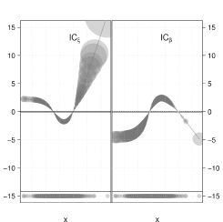
(a) Influence function of MLE

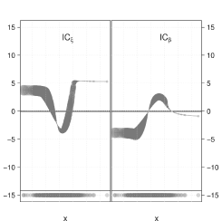
(b) Influence function of RMXE

Figure 2: Maximum likelihood and radius-minimax influence functions. On the $x$-axis the values of the observations are plotted, on the $y$-axis the respective value of the influence functions for scale and shape parameter. The influence function for the scale parameter, $\mathop{\rm IC}_{\beta}$, is scaled to $\beta$ equal to one.

The influence function quantifies the (infinitesimal) influence of each data point on the estimator. If the influence function of an estimator is unbounded, so is the GES (see Figure 2(a)), and single outliers can cause the respective estimator to produce heavily biased estimates. Robust estimators have bounded influence functions (e.g., RMXE in Figure 2(b)).

As we estimate jointly shape and scale of GPD, the influence function has two coordinates called influence curves, i.e., $\mathop{\rm IC}=(\mathop{\rm IC}_{\xi},\mathop{\rm IC}_{\beta})$. On top of the lines representing the curves themselves, we have plotted the actual observations marked as filled circles. The saturation of the points at the bottom of the graph reflects the concentration of the observations, and the radius of the points represents the size of their (joint) influence on $\xi,\beta$ in terms of $|\mathop{\rm IC}|$.

A positive [negative] value of a coordinate of the influence function at a certain observation indicates that, infinitesimally, this observation has increased [decreased] the respective value of the respective parameter coordinate. Sometimes this helps in identifying the observation(s) which has/have caused a high or low value of the parameter estimate. Also a disequilibrium of positive and negative values in a coordinate would be boldly visible. Without loss of generality, assume we have much more observations with positive value in one coordinate of the influence function, then, as the influence function must be centered, this can only happen, if there are at least some observations with a considerably negative influence.

As visible in the graphs, RMXE smoothly distributes the influence of the observations, with no outstandingly influential observations (due to boundedness). In contrast, by design, MLE cannot take into account outliers, so considers large observations as highly informative for parameter $\xi$, thereby attributing high influence to some few observations at the very right of the plot of $\mathop{\rm IC}_{\xi}$.

4.2 Outlyingness Plot

Outlyingness plots help to detect outliers, i.e., observations which deviate in some extent from the majority of data.

The plots discussed here translate ideas discussed in Hubert et al. (2005) to our GPD case; this case is not covered by the cited reference, as the model does neither fall into the scope of (multivariate) location-scale type models nor is it a regression model. Still, we follow the authors in the following two-step procedure:

In a first step, model parameters and covariances are estimated from the data by robust techniques. In the presence of outliers, classical estimators are prone to masking effects: some few large outliers may distort our quantification of outlyingness such that other (smaller) outliers no longer are identifiable; similarly, but less harmful in most cases, some “clean data” may look like outliers in the (distorted) perspective of the outlyingness measure, an effect called swamping. Robust procedures avoid both effects to large extent.

In a second step, for outlier detection, we apply an unbounded criterion to the data, e.g. the quadratic form defining the Mahalanobis norm. This unboundedness helps to discern outliers properly, which in a bounded criterion would become indistinguishable from non-outliers. However, where model parameters and covariances are needed to evaluate this criterion, e.g. the covariance to determine the Mahalanobis norm, we use the robust ones from the first step.

Usually to visualize outlyingness, two criteria from the second step are used in parallel—one of for the $x$- one for the $y$-axis. In each coordinate a threshold (preferably a suitable high quantile) is chosen, giving a partition into four quadrants. Observations simultaneously falling beyond both thresholds are flagged as outliers, which, of course, must be seen as only an indication for being an outlier, as both usual error-types of a test may occur.

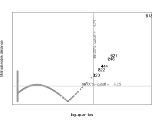
(a) Outlyingness Plot

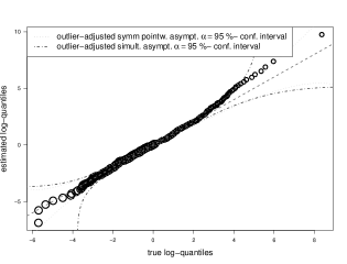
(b) QQ Plot

Figure 3: Diagnostic plots: outlyingness plot and QQ plot with robust confidence bands

There are different variations of outlying plots: distance-distance, distance-projection, and projection-projection plots. Our outlyingness plot for the GPD is a distance-projection plot, which for parameter estimation uses RMXE and for covariances the Minimum Covariance Determinant (MCD) estimator from Rousseeuw (1984), as implemented in R package rrcov, see Todorov (2009). More precisely, we plot a (robustified, empirical) Mahalanobis distance of the MLE influence function against the usual data quantiles. This gives Figure 3(a). We use thresholds given by the $99\%$ quantile of the $\chi_{2}^{2}$-distribution with non-centrality $0$ on the $y$-axis and $99\%$ quantile of the data on the $x$-axis.

Table 4 shows which operational losses in the Asset Management BL are flagged as outliers in Figure 3(a). Of the six outlying losses, indexed as $246$, $318$, $320$, $321$, $322$, $444$, four are caused by the recent fraud by B. L. Madoff and the remaining one resulted from a Ponzi scheme fraud. Although these losses are probably outliers, they should be included into the estimation instead of being skipped, as they could also carry some valuable information for future losses. Classical MLE however interprets these values as “usual observations” and, as a consequence, assigns them too much influence, no matter whether their relevance or reproducibility is doubtful or not. Robust RMXE, includes these doubtful observations too, but downweighs them, so that their influence on the resulting estimates is smaller than those of the remaining losses (see Table 3).

4.3 QQ Plot With Robust Confidence Bands

Quantile-quantile (QQ) plots aim at visualizing the quality of a model fit: empirical quantiles of the observations are plotted against the quantiles of the fitted model distribution. A concentration of the plotted points around the line $y=x$ indicates a high quality, while large deviations indicate outliers or a failure of the model fit.

Still, there is estimation uncertainty in the data, which can be captured by suitable confidence intervals grouped to bands according to their position, larger [narrower] bands indicating higher [lower] uncertainty.

As usual in this context, there are both pointwise and simultaneous confidence bands. Pointwise confidence intervals describe the stochastic variability of the empirical distributions of the data for each quantile individually, while simultaneous confidence bands capture the variability of the whole empirical cumulative distribution function (ecdf), so that, on average, $95\%$ of the graphs produced by ecdfs will completely lie within these bounds.

Taking outlier-induced model deviations into account, for robust confidence bands the nominal confidence level has to be adjusted accordingly: to warrant a nominal level $\alpha$ we have to increase the defining level to $\alpha+r/\sqrt{n}$.

The QQ plot of RMXE-estimated GPD quantiles versus real quantiles is depicted in Figure 3(b). The size of the points reflects their weight in the influence function, so that downweighed observations get smaller circles. One can see that the fit is good in the lower and middle quantiles where (at least in the middle) also model uncertainty is low, but poorer in the upper ones around $4$, where the points even fall outside the (simultaneous) confidence bands. This phenomenon appears to be due to the outlying data points in the tails (that at least get downweighed by RMXE). The widening of the confidence bands at the lower and upper ends is common and caused by the little empirical evidence available in this area.

Obs. Index Loss Value (billionsUSD ) Weight Obs. Index Loss Value (billions USD) Weight Obs. Index Loss Value (billions USD) Weight $246$ $6.0$ $0.18$ $320$ $2.4$ $0.24$ $322$ $3.3$ $0.21$ $318$ $65.0$ $0.11$ $321$ $7.2$ $0.17$ $444$ $4.0$ $0.20$

Table 3: Weights of outliers in RMXE with corresponding loss values

Outlier Index Business Line Event Type Organization Loss Amount (billions USD) Settlement Date Location 246 Asset Management Clients Products and Business Practices Amaranth Advisors 6.0 9/18/2006 North America Canada Alberta 318 Asset Management Internal Fraud Bernard Madoff Investment Services LLC 65.0 12/11/2008 North America United States New York 320 Asset Management External Fraud Ascot Partners L.P. 2.4 12/16/2008 North America United States New York 321 Asset Management External Fraud Fairfield Greenwich Group 7.2 12/15/2008 North America United States Connecticut 322 Asset Management External Fraud MassMutual Financial Group 3.3 12/16/2008 North America United States New York 444 Asset Management Internal Fraud Cash Plus 4.0 10/9/2009 Caribbean Jamaica

Table 4: Outlying events in Asset Management business line

Conclusion

This article applies optimally-robust estimation techniques to real world data for the calculation of the regulatory capital for operational risks within the LDA (AMA) setting, according to Basel II requirements. The data we use is taken from the Algo OpData database of Algorithmics Inc. No scaling has been applied, so the results we obtain are only meant for illustrative purposes.

Still, all other steps required in LDA have been gone through: we model the severity of tail events by a GPD distribution and the frequency of losses with a Poisson distribution, and apply a single-loss approximation for the corresponding $99.9\%$ quantile of the compound loss distribution. For estimation of the GPD parameters, we focus on respective optimally-robust estimators, OMSE, OBRE, and RMXE, in their specialization to the GPD case taken from Ruckdeschel and Horbenko (2010) where they are also compared with several competitors but as predicted by theory turn out optimal even at sample sizes down to $40$. For these estimators, we use a robust starting estimator, MedkMAD, based on the median and the asymmetric median of absolute deviations. Its qualification as globally robust, computationally efficient starting estimator has been taken from Ruckdeschel and Horbenko (2011).

In evaluating our estimators we have found no difficulties. In case of business line Asset Management, our robust estimators indicate the need of a higher regulatory capital than indicated by classical MLE ($28\%$ higher for RMXE), and a value of $28\%$ for the relative deviation indicates the presence of influential outliers. A statement of the type “robustly estimated OpVaR is generally higher than the one obtained by classical methods” however is not true. The order varies from business line to business line.

To assess the quality of our robust estimates and the respective model fit at real data, and to discern potential outliers, we present robust diagnostic plots. At the present data set, our outlyingness plot was able to grasp the singular pattern of the Madoff fraud. For the majority of the data, however, the robust model fit according to the QQ plot seems reasonably good. In the influence function plot, we see that at the actual data, in particular the shape parameter is concerned with highly influential observations in the MLE case, whereas no such pattern is visible in the RMXE case.

For the evaluation of the respective estimators, as well as for the diagnostic plots, we use publicly available software provided in the R package ROptEst, tuned for computational efficiency with own code, as well as own routines for the computation of MedkMAD; the code is available upon request.

References

- Balkema and de Haan (1974) Balkema, A. and de Haan, L. Residual life time at great age. Annals of Probability 2, 792–804, 1974.
- Basel II (2006) Basel Committee on Banking Supervision. International Convergence of Capital Measurement and Capital Standards: A Revised Framework. http://www.bis.org/publ/bcbs128.pdf, June, 2006.
- BIS (2010) Basel Committee on Banking Supervision. Operational Risk – Supervisory Guidelines for the Advanced Measurement Approaches. Consultative Document. http://www.bis.org/publ/bcbs184.pdf, December, 2010.
- BIS (2010a) Basel Committee on Banking Supervision. 2010 FSI Survey on the Implementation of the New Capital Adequacy Framework: Summary of responses to the Basel II implementation survey. Occasional Paper, No9. http://www.bis.org/fsi/fsipapers09.pdf, August, 2010
- Beirlant et al. (1999) Beirlant, J., Dierckx, G., Goegebeur, Y., and Matthys, G. Tail index estimation and an exponential regression model. Extremes 2, 177–200, 1999.
- Beirlant et al. (1996) Beirlant, J., Vynckier, P., and Teugels, J. L. Tail index estimation, Pareto quantile plots, and regression diagnostics. J. Amer. Statist. Assoc. 91, 1659–1667, 1996.
- Böcker and Klüppelberg (2005) Böcker, K. and Klüppelberg, C. Operational VAR: a Closed-Form Approximation. RISK Magazine, December, 90–93, 2005.
- Brazauskas and Kleefeld (2009) Brazauskas, V. and Kleefeld, A. Robust and Efficient Fitting of the Generalized Pareto Distribution with Actuarial Applications in View. Insurance: Mathematics and Economics 45, 424–435, 2009.
- Chavez-Demoulin et al. (2006) Chavez-Demoulin, V., Embrechts, P. and Neslehova, J. Quantitative models for operational risk: extremes, dependence and aggregation. Journal of Banking and Finance 30(10), 2635–2658, 2006.
- Chernobai and Rachev (2006) Chernobai, A. and Rachev, S. T. Applying Robust Methods to Operational Risk Modelling. Journal of Operational Risk 1(1), 27–41, 2006.
- Chernobai et al. (2011) Chernobai, A., Jorion, P. and Yu, F. The Determinants of Operational Risk in U.S. Financial Institutions. Journal of Financial and Quantitative Analysis. Forthcoming.
- Cope and Labbi (2008) Cope, E. and Labbi, A. Operational Loss Scaling by Exposure Indicators: Evidence from the ORX Database. Journal of Operational Risk 3(4), 2008.
- De Fontnouvelle et al. (2006) De Fontnouvelle, P., De Jesus-Rueff, V., Jordan, J. and Rosengren, E. Capital and Risk: New Evidence on Implications of Large Operational Losses. Journal of Money, Credit, and Banking 38(7), 2006.
- De Fontnouvelle et al. (2007) De Fontnouvelle, P., Rosengren, E. and Jordan, J. Implications of Alternative Operational Risk Modelling Techniques, In Carey, M. and Stulz, R. M. The Risks of Financial Institutions, University of Chicago Press, 475–512, http://www.nber.org/books/care06-1, 2007.
- Dell’Aquila and Embrechts (2009) Dell’Aquila, R. and Embrechts, P. Extremes and robustness: a contradiction? Financial Markets and Portfolio Management 20, 103–118, 2006.
- Dupuis (1998) Dupuis, D. J. Exceedances over high thresholds: A guide to threshold selection. Extremes 1(3), 251–261, 1998.
- Dupuis and Field (1998) Dupuis, D. J. and Field, C. A. Robust estimation of extremes. Canad. J. Statist. 26(2), 199–215, 1998.
- Dupuis and Morgenthaler (2002) Dupuis, D. J. and Morgenthaler S. Robust weighted likelihood estimators with an application to bivariate extreme value problems. Canad. J. Statist. 30(1), 17–36, 2002.
- Dupuis and Victoria-Feser (2006) Dupuis, D. J. and Victoria-Feser, M.-P. A robust prediction error criterion for Pareto modelling of upper tails. Canad. J. Statist. 34(4), 639–658, 2006.
- Embrechts et al. (2003) Embrechts, P., Furrer, H. and Kaufmann, R. Quantifying Regulatory Capital for Operational Risk Derivatives Use. Trading & Regulation 9(3), 217–233, 2003.
- Fernholz (1983) Fernholz, L.T., Von Mises Calculus for Statistical Functionals. Lecture Notes in Statistics, vol. 19, Springer, New York, 1983.
- Field and Smith (1994) Field, C. and Smith, B. Robust Estimation—A Weighted Maximum Likelihood Estimation. International Review 62(3), 405–424, 1994.
- Hampel et al. (1986) Hampel, F. R., Ronchetti, E. M., Rousseeuw, P. J. and Stahel, W. A. Robust statistics. The approach based on influence functions. Wiley, 1986.
- Huber (1964) Huber, P. J. Robust estimation of a location parameter. Ann. Math. Statist.35, 73–101, 1964.
- Huber (1981) Huber, P. J. Robust statistics, Wiley, 1981.
- Hubert et al. (2005) Hubert, M., Rousseeuw, P. J. and Van Aelst, S. Multivariate Outlier Detection and Robustness. Handbook of Statistics, Volume 23: Data Mining and Computation in Statistics (C. R. Rao, E. J. Wegman, J. L. Solka, Eds.), Elsevier, pp. 263–302, 2005.
- Juárez and Schucany (2004) Juárez, S. F. and Schucany, W. R. Robust and Efficient Estimation for the Generalized Pareto Distribution. Extremes 7(3), 237–251, 2004.
- Kohl et al. (2010) Kohl, M., Rieder, H., and Ruckdeschel, P. Infinitesimally Robust Estimation in General Smoothly Parametrized Models. Stat. Methods Appl., 19, 333–354, 2010.
- Kohl and Ruckdeschel (2011) Kohl, M. and Ruckdeschel, P. ROptEst: Optimally robust estimation. R package available in version 0.8 on CRAN, http://cran.r-project.org, 2011.
- Kohl and Ruckdeschel (2011) Kohl, M. and Ruckdeschel, P. distrEx: Extensions of package distr and some additional functionality. R package available in version 2.3 on CRAN, http://cran.r-project.org, 2011.
- Marazzi and Ruffieux (1999) Marazzi, A. and Ruffieux, C. The truncated mean of asymmetric distribution. Computational Statistics & Data Analysis, 32, 79–100, 1999.
- Maronna et al. (2006) Maronna, R. A., Martin, R. D. and Yohai, V. J. Robust Statistics: Theory and Methods. Wiley, 2006.
- Marshall (2001) Marshall, L. C. Measuring and Managing Operational Risks in Financial Institutions. Tools, Techniques, and other Resources. Wiley, 2001.
- Moscadelli (2004) Moscadelli, M. The modelling of operational risk: experience with the analysis of the data collected by the Basel committee. Technical Report 517, Banca d’Italia, 2004.
- Neslehova et al. (2006) Neslehova, J., Embrechts, P. and Chavez-Demoulin, V. Infinite mean models and the LDA for operational risk. Journal of Operational Risk 1(1), 3–25, 2006.
- Peng and Welsh (2001) Peng, L. and Welsh, A. H. Robust Estimation of the Generalized Pareto Distribution. Extremes 4(1), 53–65, 2001.
- Pickands (1975) Pickands, J. Statistical Inference Using Extreme Order Statistics. Annals of Statistics 3(1), 119–131, 1975.
- R Development Core Team (2011) R Development Core Team. R: A language and environment for statistical computing. R Foundation for Statistical Computing, Vienna, Austria. ISBN 3-900051-07-0, http://www.R-project.org, 2011.
- Ribatet (2009) Ribatet, M. POT: Generalized Pareto Distribution and Peaks over Threshold. R package, version 1.1-0, http://cran.r-project.org, 2009.
- Rieder (1994) Rieder, H. Robust Asymptotic Statistics. Springer, 1994.
- Rieder et al. (2008) Rieder, H., Kohl, M. and Ruckdeschel, P. The cost of not knowing the radius. Statistical Methods & Applications 17(1), 13–40, 2008.
- Rousseeuw (1984) Rousseeuw, P.J. Least Median of Squares Regression. J. Amer. Statist. Assoc. 79(388), 871–880, 1984.
- Ruckdeschel (2006) Ruckdeschel, P. A motivation for -shrinking-neighborhoods. Metrika, 63(3) 295–307, 2006.
- Ruckdeschel and Horbenko (2011) Ruckdeschel, P. and Horbenko, N. Yet another breakdown point notion: EFSBP –illustrated at scale-shape models. ArXiv 1005.1480, 2011.
- Ruckdeschel and Horbenko (2010) Ruckdeschel, P. and Horbenko, N. Robustness Properties of Estimators in Generalized Pareto Models. Technical Report ITWM No182, http://www.itwm.fraunhofer.de/fileadmin/ITWM-Media/Zentral/Pdf/Berichte_ITWM/2010/bericht_182.pdf, 2010.
- Todorov (2009) Todorov, V. rrcov: Scalable Robust Estimators with High Breakdown Point. R package, version 1.0, http://cran.r-project.org, 2009.
- Vandewalle et al. (2007) Vandewalle, B., Beirlant, J., Christmann, A., and Hubert, M. A robust estimator for the tail index of Pareto-type distributions. Comput. Statist. & Data Anal. 51(12), 6252–6268, 2007.
- van der Vaart (1998) van der Vaart, A.W. Asymptotic statistics. Cambridge Univ. Press, 1998.
- Witting (1985) Witting, H. Mathematische Statistik I: Parametrische Verfahren bei festem Stichprobenumfang. B.G. Teubner, Stuttgart, 1985.