Solutions of the Bethe-Salpeter equation in Minkowski space and applications to electromagnetic form factors

Abstract

We present a new method for solving the two-body Bethe-Salpeter equation in Minkowski space. It is based on the Nakanishi integral representation of the Bethe-Salpeter amplitude and on subsequent projection of the equation on the light-front plane. The method is valid for any kernel given by the irreducible Feynman graphs and for systems of spinless particles or fermions. The Bethe-Salpeter amplitudes in Minkowski space are obtained. The electromagnetic form factors are computed and compared to the Euclidean results.

1 Introduction

Bethe-Salpeter (BS) equation for a relativistic bound system was initially formulated in the Minkowski space [1]. It determines the binding energy and the BS amplitude. However, in practice, finding the solution in Minkowski space is made difficult due its singular behaviour. The singularities are integrable, but the standard approaches for solving integral equation fail.

To overcome this difficulty, Wick [2] formulated the BS equation in the Euclidean space, by rotating the relative energy in the complex plane $k_{0}\to ik_{4}$. This ”Wick rotation” led to a well defined integral equation which can be solved by standard methods. Most of practical applications of the BS equation have been achieved using this technique [3, 4] and recent developments make its solution a trivial numerical task [5]. Another method – the variational approach in the configuration Euclidean space – was recently developed in [6].

The binding energy provided by the Euclidean BS equation is the same than the Minkowski one. However, the Euclidean BS amplitude does not allow to calculate some observables, e.g. electromagnetic form factors. The integral providing the form factors contains singularities which are different from those appearing in the BS equation and whose positions depend on the momentum transfer. Their existence invalidates the Wick rotation in the form factor integral. In terms of the Euclidean amplitude, the form factor can be obtained only approximately, in the so called static approximation. The error rapidly increases with the momentum transfer. To avoid this problem, the knowledge of the BS amplitude in Minkowski space is mandatory.

Thus, fifty years after its formulation, finding the BS solutions in the Minkowski space is still a field of active research.

Some attempts have been recently made to obtain the Minkowski BS amplitudes. The approach proposed in [7, 8] is based on the Nakanishi integral representation [9, 10] of the amplitudes and solutions have been found for the ladder scalar case [7, 11] as well as, under some simplifying ansatz, for the fermionic one [12]. Another approach [13] relies on a separable approximation of the kernel which leads to analytic solutions. Recent applications to the $np$ system can be found in [14].

In the paper [15] we have proposed a new method to find the BS amplitude in Minkowski space and applied it to the system of two spinless particles. In [16] this approach was generalized to the two-fermion case. Like in the papers [7, 11, 12], our approach is based on Nakanishi representation of the BS amplitude. The main difference between our approach and those followed in [7, 11, 12] is the fact that, in addition to the Nakanishi representation, we use the light-front projection. This eliminates the singularities related to the BS Minkowski amplitudes. Our method is valid for any kernel given by the irreducible Feynman graphs.

In this paper we give brief review of the approach [15] to find the BS amplitude in Minkowski space, of its results and applications.

The plan of the paper is the following. In order to present the method more distinctly, we consider first the case of zero total angular momentum and spinless particles. In sect. 2, corresponding equation for the Nakanishi weight function is given. In sect. 3, it is applied to the ladder kernel and in sect. 4 – to the cross ladder one. In sect. 5 the method is generalized to the two-fermion system. Sect. 6 is devoted to application to the electromagnetic form factor, where advantage of the Minkowski space solution manifests itself in full measure. Sect. 7 contains concluding remarks.

2 Equation for the weight function

For a bound state of total momentum $p$ and in case of equal mass particles, the BS equation reads

$$\Phi(k,p)=\frac{i^{2}}{\left[(\frac{p}{2}+k)^{2}-m^{2}+i\epsilon\right]\left[(\frac{p}{2}-k)^{2}-m^{2}+i\epsilon\right]}\int\frac{d^{4}k^{\prime}}{(2\pi)^{4}}iK(k,k^{\prime},p)\Phi(k^{\prime},p),$$ (1)

where $\Phi$ is the BS amplitude, $iK$ the interaction kernel, $m$ the mass of the constituents and $k$ their relative momentum. We will denote by $M=\sqrt{p^{2}}$ the total mass of the bound state, and by $B=2m-M$ its binding energy.

Our approach consists of two steps. In the first one, the BS amplitude is expressed via the Nakanishi integral representation [9, 10]:

$$\Phi(k,p)=\int_{-1}^{1}\mbox{d}z^{\prime}\int_{0}^{\infty}\mbox{d}\gamma^{\prime}\frac{g(\gamma^{\prime},z^{\prime})}{\left[k^{2}+p\cdot k\;z^{\prime}+\frac{1}{4}M^{2}-m^{2}-\gamma^{\prime}+i\epsilon\right]^{3}}.$$ (2)

Notice that in this representation, the dependence on the two scalar arguments $k^{2}$ and $p\makebox[2.27626pt]{$\cdot$}k$ of the BS amplitude is made explicit by the integrand denominator and that the weight Nakanishi function $g(\gamma,z)$ is non-singular. By inserting the amplitude (2) into the BS equation one finds an integral equation, still singular, for $g$.

In the second step, we apply to both sides of BS equation an integral transform – light-front projection [15] – which eliminates singularities of the BS amplitude. It consists in replacing $k\to k+\frac{\omega}{\omega\makebox[2.27626pt]{$\cdot$}p}\,\beta$ where $\omega$ is a light-cone four-vector $\omega^{2}=0$, and integrating over $\beta$ in infinite limits. We obtain in this way, a non-singular equation for the non-singular $g(\gamma,z)$. After solving it and substituting the solution in eq. (2), the BS amplitude in Minkowski space can be easily computed.

This leads (see ref. [15] for the detail of calculations) to the following equation for the weight function $g(\gamma,z)$:

$$\int_{0}^{\infty}\frac{g(\gamma^{\prime},z)d\gamma^{\prime}}{\Bigl{[}\gamma^{\prime}+\gamma+z^{2}m^{2}+(1-z^{2})\kappa^{2}\Bigr{]}^{2}}=\int_{0}^{\infty}d\gamma^{\prime}\int_{-1}^{1}dz^{\prime}\;V(\gamma,z;\gamma^{\prime},z^{\prime})g(\gamma^{\prime},z^{\prime}),$$ (3)

This is just the eigenvalue equation of our method. It is equivalent to the initial BS equation (1). The total mass $M$ of the system appears on both sides of equation (3) and is contained in the parameter $\kappa^{2}=m^{2}-\frac{1}{4}M^{2}.$ As calculations [7, 8] show, $g(\gamma,z)$ may be zero in an interval $0\leq\gamma\leq\gamma_{0}$. The exact value where it differs from zero is determined by the equation (3) itself.

The kernel $V$, appearing in the right-hand side of eq. (3), is related to the kernel $iK$ from the BS equation by

$$V(\gamma,z;\gamma^{\prime},z^{\prime})=\frac{\omega\cdot p}{\pi}\int_{-\infty}^{\infty}\frac{-iI(k+\beta\omega,p)d\beta}{\left[(\frac{p}{2}+k+\beta\omega)^{2}-m^{2}+i\epsilon\right]\left[(\frac{p}{2}-k-\beta\omega)^{2}-m^{2}+i\epsilon\right]},$$ (4)

with

$$I(k,p)=\int\frac{d^{4}k^{\prime}}{(2\pi)^{4}}\frac{iK(k,k^{\prime},p)}{\left[{k^{\prime}}^{2}+p\cdot k^{\prime}z^{\prime}-\gamma^{\prime}-\kappa^{2}+i\epsilon\right]^{3}}.$$ (5)

For simple kernels $K(k,k^{\prime},p)$ given by a Feynman graph the integral (5) over $k^{\prime}$ is calculated analytically. The integral (4) over $\beta$ is also calculated analytically and it is expressed via residues. The singularities in the BS equation are removed by the analytical integration over $\beta$. Equation (3) is valid for an arbitrary kernel $iK$, given by a Feynman graph. The particular cases of the ladder kernel and of the Wick-Cutkosky model [2, 17] are detailed in the next section and for the cross ladder kernel – in the paper [18]. Once $g(\gamma,z)$ is known, the BS amplitude can be restored by eq. (2).

The variables ($\gamma,z$) are related to the standard light front (LF) variables as $\gamma=k_{\perp}^{2}$, $z=1-2x$. The LF wave function (see its definition in [19], for instance) can be easily obtained by [15]:

$$\psi(k_{\perp},x)=\frac{1}{\sqrt{4\pi}}\int_{0}^{\infty}\frac{x(1-x)g(\gamma^{\prime},1-2x)d\gamma^{\prime}}{\Bigl{[}\gamma^{\prime}+k_{\perp}^{2}+m^{2}-x(1-x)M^{2}\Bigr{]}^{2}}.$$ (6)

Eq. (3) can be transformed, in principle, to the equation for the LF wave function $\psi(k_{\perp},x)$, though this requires inverting the kernel in the left-hand side of (3). The initial BS equation (1), projected on the LF plane, can be also approximately transformed to the LF equation:

$$\left(\frac{\vec{k}^{2}_{\perp}+m^{2}}{x(1-x)}-M^{2}\right)\psi(\vec{k}_{\perp},x)=-\frac{m^{2}}{2\pi^{3}}\int\psi(\vec{k}^{\prime}_{\perp},x^{\prime})V_{LF}(\vec{k}^{\prime}_{\perp},x^{\prime};\vec{k}_{\perp},x,M^{2})\frac{d^{2}k^{\prime}_{\perp}dx^{\prime}}{2x^{\prime}(1-x^{\prime})}$$ (7)

with the LF kernel $V_{LF}$ given, for ladder exchange, in ref. [15].

It is worth noticing that the LF wave function (6) is different from the one obtained by solving the ladder LF equation (7), as it was done e.g. in ref. [20]. The physical reason lies in the fact that the iterations of the ladder BS kernel (Feynman graphs) and the ladder LF kernel (time-ordered graphs) generate different intermediate states. The LF kernel and its iterations contain in the intermediate state only one exchanged particle, whereas the iterations of the ladder Feynman kernel contain also, many-body states with increasing number of exchanged particles (stretched boxes). This leads to a difference in the binding energies, which is however small [20]. Formally, this difference arises because of the approximations which are made in deriving eq. (7) from (1). However, for a kernel given by a finite set of irreducible graphs, both BS (1) and LF (7) equations are already approximate and it is not evident which of them is more ”physical”. The physically transparent interpretation of the LF wave function makes it often more attractive.

3 Spinless particles. Ladder kernel

As illustration, we give here the kernel $V(\gamma,z;\gamma^{\prime},z^{\prime})$ of equation (3) for the ladder BS kernel, which reads:

$$iK^{(L)}(k,k^{\prime},p)=\frac{i(-ig)^{2}}{(k-k^{\prime})^{2}-\mu^{2}+i\epsilon}.$$ (8)

We substitute it in eq. (5), then substitute (5) in (4) and calculate the integrals. The details of these calculations are given in ref. [15] and one obtains:

$$V(\gamma,z;\gamma^{\prime},z^{\prime})=\left\{\begin{array}[]{ll}W(\gamma,z;\gamma^{\prime},z^{\prime}),&\mbox{if $-1\leq z^{\prime}\leq z\leq 1$}\\ W(\gamma,-z;\gamma^{\prime},-z^{\prime}),&\mbox{if $-1\leq z\leq z^{\prime}\leq 1$}\end{array}\right.$$ (9)

where $W$ has the form:

$$W(\gamma,z,\gamma^{\prime},z^{\prime})=\frac{\alpha m^{2}}{2\pi}\;\frac{(1-z)^{2}}{D_{0}}\;\int_{0}^{1}\frac{v^{2}}{D^{2}}\;dv$$ (10)

with $\alpha=g^{2}/(16\pi m^{2})$ and

$$D_{0} = \gamma+m^{2}z^{2}+(1-z^{2})\kappa^{2}$$

$$D = v(1-v)(1-z^{\prime})\gamma+(1-z)[(1-v)\mu^{2}+v\gamma^{\prime}]$$

$$+ vm^{2}\;[(1-v)(1-z^{\prime})z^{2}+v{z^{\prime}}^{2}(1-z)\;]+v\kappa^{2}(1-z)(1-z^{\prime})\;[1+z-v(z-z^{\prime})\;]$$

In the particular case we are considering here, the angular integral over $v$ can be performed analytically and $W$ obtains the simple expression:

$$W(\gamma,z;\gamma^{\prime},z^{\prime}) = \frac{\alpha m^{2}}{2\pi}\frac{(1-z)^{2}}{\gamma+z^{2}m^{2}+(1-z^{2})\kappa^{2}}$$

$$\times \frac{1}{b_{2}^{2}(b_{+}-b_{-})^{3}}\left[\frac{(b_{+}-b_{-})(2b_{+}b_{-}-b_{+}-b_{-})}{(1-b_{+})(1-b_{-})}+2b_{+}b_{-}\log\frac{b_{+}(1-b_{-})}{b_{-}(1-b_{+})}\right]$$

$$b_{\pm} = -\frac{1}{2b_{2}}\;\left(b_{1}\pm\sqrt{b_{1}^{2}-4b_{0}b_{2}}\right),\qquad b_{0}\;=\;(1-z)\mu^{2},$$

$$b_{1} = \gamma+\gamma^{\prime}-(1-z)\mu^{2}-\gamma^{\prime}z-\gamma z^{\prime}+(1-z^{\prime})\left[z^{2}m^{2}+(1-z^{2})\kappa^{2}\right],$$

$$b_{2} = -\gamma(1-z^{\prime})-(z-z^{\prime})\left[(1-z)(1-z^{\prime})\kappa^{2}+(z+z^{\prime}-zz^{\prime})m^{2}\right].$$

One can show [15] that in the case $\mu=0$, which constitutes the original Wick-Cutkosky model [2, 17], the solution has the form $g(\gamma,z)=\delta(\gamma)\;g(z)$. The $\gamma$-dependence disappears from the equation which, after that, exactly coincides with the Wick-Cutkosky equation [2, 3, 17].

Table 1: Coupling constant values as a function of the binding energy for $\mu=0.15$ and $\mu=0.5$ obtained with $\gamma_{max}=3$, $N_{\gamma}=12$, $N_{z}=10$ and $\varepsilon_{R}=10^{-6}$.

$B$	$\alpha(\mu=0.15)$	$\alpha(\mu=0.50)$
0.01	0.5716	1.440
0.10	1.437	2.498
0.20	2.100	3.251
0.50	3.611	4.901
1.00	5.315	6.712

Equation (3) has been solved by using the method explained in Appendix A, i.e. by expanding the solution $g$ on a bicubic cubic spline basis. By keeping $\varepsilon_{R}=10^{-6}$ fixed and varying the grid parameters to ensure four digits accuracy, we obtain for $\mu=0.15$ and $\mu=0.5$ and unit constituent mass ($m=1$) the values displayed in table 1. They correspond to $\gamma_{max}=3$, $N_{\gamma}=12$, $N_{z}=10$. With all shown digits, they are in full agreement with the results we have obtained, similarly to [20], by using the Wick rotation and the method of [5]. Increasing $\varepsilon_{R}$ to $10^{-4}$ changes at most one unit in the last digit. This demonstrates the validity of our approach.

The weight function $g$ for a system with $\mu=0.5$ and $B=1.0$ is plotted in fig. 1. It has been obtained with $\varepsilon_{R}=10^{-4}$ and the same grid parameters than in table 1. Its $\gamma$-dependence is not monotonous and has a nodal structure; the $z$-variation is also non trivial. We have remarked a strong dependence of $g(\gamma,z)$ relative to values of the $\varepsilon_{R}$ parameter smaller than $\sim 10^{-4}$, in contrast to high stability of corresponding eigenvalues. However the corresponding BS amplitude $\Phi$ and LF wave function $\psi$, obtained from $g(\gamma,z)$ by the integrals (2) and (6), show the same strong stability as the eigenvalues.

Figure 1: Nakanishi function $g(\gamma,z)$ for $\mu=0.5$ and $B=1.0$. On left – versus $\gamma$ for fixed values of $z$ and on right – versus $z$ for a few fixed values of $\gamma$.

The BS amplitude in Minkowski space in the rest frame $\vec{p}=0$ is shown in fig. 2. The $k$-dependence is rather smooth but the $k_{0}$-dependence, due to poles of the propagators in (1), exhibits a singular behaviour at $k_{0}=\pm\left(\varepsilon_{k}\pm\frac{M}{2}\right)$, i.e. moving with $\vec{k}$ and $M$.

Figure 2: BS amplitude $\Phi(k_{0},k)$ for $\mu=0.5$ and $B=1.0$. On left versus $k$ for fixed values of $k_{0}$ and on right versus $k_{0}$ for a few fixed values of $k$.

Note that our solution gives also the BS amplitude in Euclidean space, by substituting in (2) $k_{0}=ik_{4}$. It is indistinguishable from the one obtained by a direct solution of the Wick-rotated BS equation [15].

4 Spinless particles. Cross ladder kernel

Non-ladder effects, within the same model, using Feynman-Schwinger representation, were considered in ref. [22]. In this work the full set of all irreducible cross-ladder graphs in a bound state calculation was included. Refs. [23, 24] contain results on the binding energy found by solving the BS equation for (L+CL) in Euclidean space. In the LFD framework, binding energy for (L+SB) kernel is calculated in [25], whereas the (L+CL+SB) contribution is incorporated in [24]. In [26] the effect of the cross-ladder graphs in the BS framework was estimated with the kernel represented through a dispersion relation. Non-ladder self-energy effects have been incorporated in [27, 28, 11].

Figure 3: Feynman cross graph.

As mentioned, the equation (3) is valid for any kernel. Derivation of $V$ in this equation for the cross-ladder BS kernel, shown in fig. 3, is quite similar but more lengthy, since the kernel itself is more complicated. We have first to calculate to the kernel $K^{(CL)}(k,k^{\prime},p)$ corresponding to the diagram in fig. 3, substitute the result in (5), then in (4) and find in this way the cross-ladder contribution to the kernel $V(\gamma,z;\gamma^{\prime},z^{\prime})$ in equation (3). The full kernel – including ladder and cross-ladder graphs – will be written in the form:

$$V(\gamma,z;\gamma^{\prime},z^{\prime})=V^{(L)}(\gamma,z;\gamma^{\prime},z^{\prime})+V^{(CL)}(\gamma,z;\gamma^{\prime},z^{\prime}).$$

The ladder kernel $V^{(L)}$ is given in refs. [15, 19]. The cross-ladder contribution $V^{(CL)}$ was calculated in the paper [18].

We compare the results obtained in the BS approach with the equivalent ones found in Light-Front Dynamics (LFD). The latter incorporates the graphs with two bosons in flight forming six cross boxes and two stretched boxes. They were also calculated in [18],

     

Figure 4: On left: Binding energy $B$ vs. coupling constant $\alpha$ for BS and LF equations with the ladder (L) kernels only and with the ladder +cross-ladder (L+CL) one for exchange mass $\mu=0.15$. On right: The same as on left but for exchange mass $\mu=0.5$ and, in addition, binding energy $B$ for LF equation with the ladder +cross-ladder +stretched box (L+CL+SB) kernel.

The binding energy $B$ as a function of the coupling constant $\alpha$ is shown in figures 4 for exchange masses $\mu=0.15$ and $\mu=0.5$ respectively and $m=1$.

We see that for the same kernel – ladder or (ladder + cross-ladder) – and exchange mass – $\mu=0.15$ or $\mu=0.5$ – the binding energies obtained by BS and LFD approaches are very close to each other. The BS equation is slightly more attractive than LFD. At the same time, the results for ladder and (ladder +cross-ladder) kernels considerably differ from each other. The effect of the cross-ladder is strongly attractive. Though the stretched box graphs are included, its contribution to the binding energy is smaller than 2% and attractive as well.

The zero binding limit of fig. 4 deserves some comments. It was found in [20] that for massive exchange, the relativistic (BS and LF) ladder results do not coincide with those provided by the Schrödinger equation and the corresponding non relativistic kernel (Yukawa potential) even at very small binding energies. Their differences increase with the exchanged mass $\mu$ and do not vanish in the limit $B\to 0$. We have displayed in fig. 5 a zoom of fig. 4 (right) for small values of $B$. The cross ladder and stretched box diagrams reduce the differences but are not enough to cancel it.

We see that the cross-ladder contribution, relative to the ladder one, results in a strong attractive effect. The BS and LFD approaches give very close results for any kernel, with BS equation being always more attractive. These approaches differ from each other by the stretched-box diagrams with higher numbers of intermediate mesons. Our results indicate that the higher order stretched box contributions are small. This agrees with direct calculations in LFD of stretched box kernel with two-meson states [29] and with calculations of the higher Fock sector contributions [30] in the Wick-Cutkosky model. Calculation in LFD of binding energy with the stretched box contribution (L+CL+SB) and its comparison with (L+CL) also shows that the stretched box contribution is attractive but small.

Figure 5: Zoom of figure 4 (right) in the zero binding energy region. The ladder and (ladder +cross ladder +stretched box) results obtained with the LF equation are compared to the non relativistic ones (Schrodinger equation with Yukawa potential).

The comparison of our results with those obtained in [22], evaluating the binding energy $B_{all}$ for the complete set of all irreducible diagrams, shows that the effect of the considered cross ladder graphs, though being very important, represent only a small part of the total correction. Thus for $\mu=0.15$ and $\alpha=0.9$ the corresponding binding energies obtained with BS equation are $B_{L}\approx 0.035$, $B_{L+CL}\approx 0.06$ and $B_{all}\approx 0.225$.

Qualitatively, our large attractive effect of CL (for $\mu=0.15$ and $\mu=0.5$) is in agreement with [23] (where $\mu=1$). For $\mu=0.15$, our numerical results for binding energy, both for the BS equation in Minkowski space and in the LFD approach, are close to those found in [24] (within accuracy of extracting the data from plots). Our results are smaller than the ones found in [26] by a factor 3.

5 Two fermions

We have considered the following fermion ($\Psi,m$) - meson ($\phi,\mu$) interaction Lagrangians:

(i) Scalar coupling ${\cal L}_{int}^{(s)}=g\,\bar{\Psi}\phi\,\Psi$ for which $\Gamma_{\alpha}=ig$

(ii) Pseudoscalar coupling ${\cal L}_{int}^{(ps)}=ig\,\bar{\Psi}\gamma_{5}\phi\,\Psi$ for which $\Gamma_{\alpha}=-g\gamma_{5}$.

(ii) Massless vector exchange ${\cal L}_{int}^{(v)}=\bar{\Psi}\gamma^{\mu}V^{\mu}\,\Psi$ with $\Gamma_{\alpha}=ig\gamma^{\mu}$ and $\Pi_{\mu\nu}=-i{g_{\mu\nu}/q^{2}}$ as vector propagator.

Each interaction vertex has been regularized with a vertex form factor $F(k-k^{\prime})$ by the replacement $g\to gF(k-k^{\prime})$ and we have chosen $F$ in the form:

$$F(q)=\frac{\mu^{2}-\Lambda^{2}}{q^{2}-\Lambda^{2}+i\epsilon}.$$ (12)

Let us first consider the case of the scalar coupling and the corresponding ladder kernel. The BS equation for the amplitude $\Phi$ reads:

$$\Phi(k,p)=\frac{i(m+\frac{1}{2}\hat{p}+\hat{k})}{(\frac{1}{2}p+k)^{2}-m^{2}+i\epsilon}\left[\int\frac{\mbox{d}^{4}k^{\prime}}{(2\pi)^{4}}\;\Phi(k^{\prime},p)\frac{(-ig^{2})\,F^{2}(k-k^{\prime})}{(k-k^{\prime})^{2}-\mu^{2}+i\epsilon}\right]\frac{i(m-\frac{1}{2}\hat{p}+\hat{k})}{(\frac{1}{2}p-k)^{2}-m^{2}+i\epsilon}.$$ (13)

In the case of $J^{\pi}=0^{+}$ state, the BS amplitude has the following general form:

$$\Phi(k,p)=S_{1}\phi_{1}+S_{2}\phi_{2}+S_{3}\phi_{3}+S_{4}\phi_{4}$$ (14)

where $S_{i}$ are independent spin structures ($4\times 4$ matrices) and $\phi_{i}$ are scalar functions of $k^{2}$ and $p\cdot k$. The choice of $S_{i}$ is to some extent arbitrary. To benefit from useful orthogonality properties we have taken

$$S_{1}=\gamma_{5},\quad S_{2}=\frac{1}{M}\hat{p}\,\gamma_{5},\quad S_{3}=\frac{k\cdot p}{M^{3}}\hat{p}\,\gamma_{5}-\frac{1}{M}\hat{k}\,\gamma_{5},\quad S_{4}=\frac{i}{M^{2}}\sigma_{\mu\nu}p_{\mu}k_{\nu}\,\gamma_{5},$$

where $\sigma_{\mu\nu}=\frac{i}{2}(\gamma_{\mu}\gamma_{\nu}-\gamma_{\nu}\gamma_{\mu})$. The antisymmetry of the amplitude (14) with respect to the permutation $1\leftrightarrow 2$ implies for the scalar functions: $\phi_{1,2,4}(k,p)=\phi_{1,2,4}(-k,p)$, $\phi_{3}(k,p)=-\phi_{3}(-k,p)$. A decomposition similar to (14) was used in [12] to solve the BS equation for a quark-antiquark system but the solution was approximated keeping only the first term $S_{1}\phi_{1}$.

We substitute (14) in eq. (13), multiply it by $S_{i}$ and take traces. As we will see, the kernel in the resulted equation, in contrast to the spinless case, is still singular. These singularities are integrable numerically. They do not prevent from finding numerical solution, but they reduce its precision. This can be avoided by a proper regularization of equation, multiplying both sides of it by the factor

$$\eta(k,p)=\frac{(m^{2}-L^{2})}{\left[(\frac{p}{2}+k)^{2}-L^{2}+i\epsilon\right]}\frac{(m^{2}-L^{2})}{\left[(\frac{p}{2}-k)^{2}-L^{2}+i\epsilon\right]}$$ (15)

This factor has the form of a product of two scalar propagators with mass $L$. It plays the role of form factor suppressing the high off-mass shell values of the constituent four-momenta $k^{2}_{1,2}=(\frac{p}{2}\pm k)^{2}$ and tends to 1 when $L\to\infty$. In this way, we get the following system of equations for the invariant functions $\phi_{i}$:

$$\eta(k,p)\;\phi_{i}(k,p) = \frac{\eta(k,p)}{[(\frac{p}{2}+k)^{2}-m^{2}+i\epsilon][(\frac{p}{2}-k)^{2}-m^{2}+i\epsilon]}$$ (16)

$$\times \int\frac{\mbox{d}^{4}k^{\prime}}{(2\pi)^{4}}\frac{ig^{2}\,F^{2}(k-k^{\prime})}{(k-k^{\prime})^{2}-\mu^{2}+i\epsilon}\sum_{j=1}^{4}c_{ij}(k,k^{\prime},p)\phi_{j}(k^{\prime},p),$$

Since $\eta(k,p)\neq 0$, the equation thus obtained is strictly equivalent to one where $\eta(k,p)$ is cancelled. We will see however that, due to the presence of the $\eta$ factor, the LF projection modifies the resulting kernels which become less singular functions.

The coefficients $c_{ij}$ are determined by traces. We do not give here their explicit form, which can be found in [16].

Then we represent each of the BS components $\phi_{i}(k,p)$ by means of the Nakanishi integral (2) and, similarly to the scalar case, apply the light-front projection to the set of coupled equations for the corresponding weight functions $g_{i}(\gamma,z)$. As explained in sect. 2, this projection, which is an essential ingredient of our works [15, 18, 31], consists in replacing $k\to k+\frac{\omega}{\omega\cdot p}\beta$ in eq. (16) and integrating over $\beta$ in all the real domain.

The technical details of the light-front projection are similar to those given in ref. [15]. We obtain in this way a set of coupled two-dimensional integral equations:

$$\int_{0}^{\infty}\mbox{d}\gamma^{\prime}\int_{-1}^{1}\mbox{d}z^{\prime}\;V^{g}(\gamma,z;\gamma^{\prime},z^{\prime})\;g_{i}(\gamma^{\prime},z^{\prime})=\sum_{j}\int_{0}^{\infty}\mbox{d}\gamma^{\prime}\int_{-1}^{1}\mbox{d}z^{\prime}\;V^{d}_{ij}(\gamma,z;\gamma^{\prime},z^{\prime})g_{j}(\gamma^{\prime},z^{\prime})$$ (17)

The kernel $V^{g}$ and also $V^{d}_{ij}$ for all types of couplings and states are given in [16]. These kernels depend on the parameter $L$. Closer is $L$ to $m$, smoother is the kernel and more stable are the numerical solutions. However the weight functions $g_{i}(\gamma,z)$ as well as binding energies provided by (17) are independent of $L$. To avoid spurious singularities in (17) due to the $\eta$ factor (15), $L^{2}$ must be larger than $\frac{M^{2}}{2}-m^{2}$, what is fulfilled for $L>m$. In practical calculations we have taken $m=1$ and $L=1.1$.

The kernel $V_{g}$ is finite and it vanishes for $z=\pm 1$. For a fixed values of $\gamma,z$ and $\gamma^{\prime}$, $V_{g}$ is a continuous function of $z^{\prime}$ with a discontinuous derivative at $z^{\prime}=z$.

Figure 6: Left: kernel matrix elements $V_{14}(\gamma,z;\gamma^{\prime},z^{\prime})$ for $z=0.7,0.9,0.95$ as a function of $z^{\prime}$ and fixed values of $\gamma,\gamma^{\prime}$. The discontinuity is finite at a fixed value of $z$ but diverges when $z\to 1$. Right: regularized kernel $V^{d}_{14}$, plotted for the same arguments and $L=1.1m$.

As already mentioned, without $\eta$-factor, most of the kernel matrix elements $V^{d}_{ij}$ are singular. Namely, they are discontinuous at $z^{\prime}=z$. In some cases – like e.g. $V_{14}$ displayed in fig. 6 (left) – the value of the discontinuity, although being finite at fixed value of $z$, diverges when $z\to\pm 1$. This creates some numerical difficulties when computing the solutions $g_{i}(\gamma,z)$ in the vicinity of $z=\pm 1$. They can be in principle solved by properly taking into account the particular type of divergence. However the latter may depend on the particular matrix element, on the type of coupling, the quantum number of the state and other details of the calculation.

For $\eta\neq 1$, i.e., for a finite value of $L$ in (15), the $z^{\prime}$-dependence of the regularized kernels is much more smooth and therefore better adapted for obtaining accurate numerical solutions. In fig. 6 (right) we plotted the regularized kernel $V^{d}_{14}$ as a function of $z^{\prime}$ for the same arguments $\gamma,z,\gamma^{\prime}$ and parameters than in fig. 6 (left), where it was calculated without the $\eta(k,p)$ factor. As one can see, the kernel is now a continuous function of $z^{\prime}$. A discontinuity of the first derivative however remains at $z^{\prime}=z$.

We would like to emphasize again that despite the fact that the non-regularized and regularized kernels are very different from each other (compare e.g. figs. 6 left and right) and that the regularized ones strongly depends on the value of $L$, they provide – up to numerical errors – the same binding energies and weight functions $g_{i}(\gamma,z)$. We construct in this way a family of equivalent kernels.

Table 2: Left: Coupling constant $g^{2}$ as a function of binding energy $B$ for the $J=0$ state with scalar (S), pseudoscalar (PS) and massless vector (positronium) exchange kernels. The vertex form factor is $\Lambda=2$ and the parameter of the $\eta$ factor $L=1.1$. Right: Coupling constant $g^{2}$ as a function of binding energy $B$ for the positronium $J=0$ state in BS equation in the region of stability without vertex form factor ($\Lambda\to\infty$), i.e. $g<\pi$. They are compared to the non relativistic results.

	S		PS		positronium
$\mu$	0.15	0.50	0.15	0.50	0.0
$B$	$g^{2}$	$g^{2}$	$g^{2}$	$g^{2}$	$g^{2}$
0.01	7.813	25.23	224.8	422.3	3.265
0.02	10.05	29.49	232.9	430.1	4.910
0.03	11.95	33.01	238.5	435.8	6.263
0.04	13.69	36.19	243.1	440.4	7.457
0.05	15.35	39.19	247.0	444.3	8.548
0.10	23.12	52.82	262.1	459.9	13.15
0.20	38.32	78.25	282.9	480.7	20.43
0.30	54.20	103.8	298.6	497.4	26.50
0.40	71.07	130.7	311.8	515.2	31.84
0.50	86.95	157.4	323.1	525.9	36.62

$B$	$g^{2}_{NR}$	$g^{2}_{BS}$
0.01	2.51	3.18
0.02	3.55	4.65
0.03	4.35	5.75
0.04	5.03	6.64
0.05	5.62	7.38
0.06	7.95	8.02
0.07	11.24	8.57
0.08	13.77	9.06
0.09	15.90	9.49

The solutions of eq. (17) have been obtained using the techniques detailed in Appendix A. We have computed the binding energies and BS amplitudes, for the $J=0^{+}$ two fermion system interacting with massive scalar (S) and pseudoscalar (PS) exchange kernels and for the fermion-antifermion system interacting with massless vector exchange in Feynman gauge. In the limit of an infinite vertex form factor parameter $\Lambda\to\infty$, the later case would correspond to positronium with an arbitrary value of the coupling constant. All the results presented in this section are given in the constituent mass units ($m=1$) and with $L=1.1$.

The binding energies obtained with the form factor parameter $\Lambda=2$ are given in left table 2. For the scalar and pseudoscalar cases, we present the results for $\mu=0.15$ and $\mu=0.50$ boson masses. They have been compared to those obtained in a previous calculation in Euclidean space [32] using a slightly different form factor, which differs from our one by a factor. Once taken into account this correction, our scalar results are in full agreement (four digits) with [32]. The pseudoscalar ones show small discrepancies ($\approx 0.5\%$). We have also computed the binding energies by directly solving the fermion BS equation the Euclidean space using a method independent of the one used in [32]. Our Euclidean results are in full agreement with those given in the table 2.

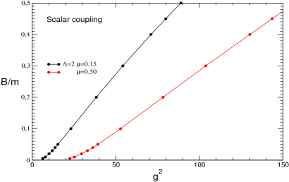
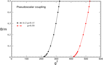
Figure 7: Left: Binding energy for scalar exchange v.s. $g^{2}$ for $\Lambda=2$, $L=1.1$, $\mu=0.15$ and $\mu=0.5$. Right: Binding energy for pseudo scalar exchange v.s. $g^{2}$ for $\Lambda=2$, $L=1.1$, $\mu=0.15$ and $\mu=0.5$.

The $B(g^{2})$ dependence for the scalar and pseudoscalar couplings is plotted in figs. 7. Notice the different $g^{2}$ scales of both dependences. The pseudoscalar binding energies are fast increasing functions of $g^{2}$ and thus more sensitive to the accuracy of numerical methods. This sharp behaviour was also exhibit when solving the corresponding LF equation [33].

It is worth noticing that the stability properties of the BS $J^{\pi}=0^{+}$ solutions for the scalar coupling are very similar to the LF ones. In the latter case, we have shown [34, 35] the existence of a critical coupling constant $g_{c}$ below which the system is stable without vertex form factor while for $g>g_{c}$, the system ”collapses”, i.e. the spectrum is unbounded from below. The numerical value was found to be $\alpha_{c}=3.72$ [34, 35], which corresponds to $g_{c}=6.84$. Performing the same analysis than in our previous work – eq. (71) from [34, 35] – we found that for BS equation the critical coupling constant is $g_{c}=2\pi$, in agreement with [32]. The $10\%$ difference between the numerical values of $g_{c}$ is apparently due to the different contents of the intermediate states in the two approaches. The ladder BS equation incorporates effectively the so-called stretch-boxes diagrams which are not taken into account in the ladder LF results.

The positronium case deserves some comments. First we would like to notice that in our formalism, the singularity of the Coulomb-like kernels in terms of the momentum transfer $1/(k-k^{\prime})^{2}$ is absent. This is a combined consequence of the Nakanishi transform (2) – which allows to integrate over $k^{\prime}$ analytically in the right hand side of the BS equation (16) – and of the consecutive LF projection integral. After this integration, the Coulomb singularity does not anymore manifest itself in the kernel. This can be explicitly seen in the kernel of the Wick-Cutkosky model obtained in eq. (22) of our previous work [15].

A second remark concerns the $\Lambda$ dependence of the positronium results. Using the methods developed in [34, 35] we found that in the BS approach with ladder kernel there also exists a critical value of the coupling constant $g_{c}=\pi$. Note that, as in the scalar coupling, the very existence and the value of this critical coupling constant is independent on the constituent ($m$) and exchange $\mu$ masses but depends on the quantum number of the state.

The ground state positronium binding energies without vertex form factor are given in the left table 2 for values of the coupling below $g_{c}$, Nonrelativistic results $g^{2}_{NR}=8\pi\sqrt{B/m}$ are included for comparison. One can see that the relativistic effects are repulsive.

These results are displayed in fig. 8 (left), black solid line, and compared to the binding energies obtained with two values of the form factor parameter $\Lambda=2$ (dashed) and $\Lambda=5$ (dot-dashed). The stability region is limited by a vertical dotted line at $g=g_{c}=\pi$. Beyond this value the binding energy without form factor becomes infinite and we have found $B(g\to g_{c})\approx 0.10$.

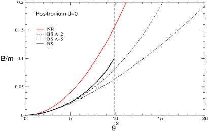
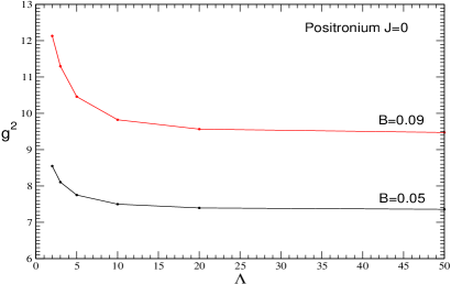
Figure 8: Left: Binding energy for J=0 positronium state versus $g^{2}$ (black solid line) in the stability region $g<g_{c}=\pi$. Dashed and dotted-dashed curves correspond to the results for increasing values of the vertex form factor parameter $\Lambda$. They are compared to the non relativistic results (red solid line). Right: $\Lambda$-dependence of $g^{2}$ for for $J=0$ positronium state for fixed values of binding energies $B=0.1$ and $B=0.5$.

The inclusion of the form form factor has a repulsive effect, i.e. for a fixed value of the coupling constant it provides a binding energy of the system which is smaller than in the $\Lambda\to\infty$ limit (no cut-off). This is also illustrated in fig. 8 (right) where we have plotted the $\Lambda$ dependence of $g^{2}$ for two different energies. One can see that the value of the coupling constant to produce a bound state is a decreasing function of $\Lambda$. The size of the effect depends strongly on the binding energy but for both energies the asymptotics is reached at $\Lambda\approx 20$. This behaviour is understandable in terms of regularizing the short range singularity of $-1/r^{2}$ interactions.

     

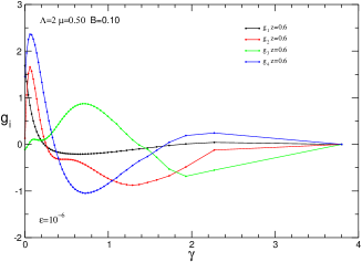
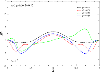
Figure 9: Left: Nakanishi weight functions v.s. $\gamma$ for $z=0.6$, for scalar exchange for $\Lambda=2$, $L=1.1$, $\mu=0.15$ and $\mu=0.5$. Right: Nakanishi weight functions v.s. $z$ for $\gamma=0.54$.

We present in figs. 9 some examples of the Nakanishi weigh functions $g_{i}(\gamma,z)$. They correspond to a $B=0.1$ state with the scalar coupling and the same parameters $\Lambda=2$, $\mu=0.50$ than in table 2. In the left figure is shown the $\gamma$-dependence for a fixed value of $z$ and in the right figure the $z$-dependence for a fixed $\gamma$. Notice the regular behaviour of these functions as well as their well defined parity with respect to $z$ – $g_{1,2,4}$ are even and $g_{3}$ is odd. As in the scalar case, the $\varepsilon_{R}$-dependence of $g_{i}$ is more important than for the binding energy.

Corresponding BS amplitudes $\phi_{i}$ are displayed in figs. 10. The figure 10 (left) represents the $k_{0}$ dependence of $\phi_{i}$ for a fixed value of $\mid\vec{k}\mid=0.2$. They exhibit a singular behaviour which corresponds to the pole of free propagators $k_{0}=\epsilon_{k}-\frac{M}{2}$, like in the scalar case. The figure 10 (right) represents the $\mid\vec{k}\mid$ dependence of the amplitudes $\phi_{i}$ for a fixed value $k_{0}=0.04$. For this choice of arguments, the amplitudes are smooth functions of $\mid\vec{k}\mid$, though they will be also singular for $k_{0}>\frac{B}{2}=0.05$. Notice that all the infinities in the BS amplitudes $\phi_{i}$ come from the free propagator. However the BS amplitude has other non-analytical points. For instance it obtains an imaginary part for $(\frac{p}{2}\pm k)^{2}>(m+\mu)^{2}$.

     

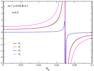
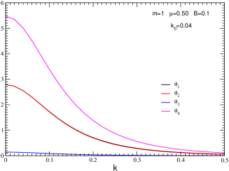
Figure 10: Bethe-Salpeter Minkowski amplitudes, corresponding to figs. 9, v.s. $k_{0}$ for $k=|\vec{k}|=0.2$ (on left) and v.s. $k=|\vec{k}|$ for $k_{0}=0.04$ (on right). The amplitudes $\phi_{1}$ and $\phi_{2}$ are indistinguishable.

6 Electromagnetic form factor

We demonstrate in this section the advantages of using the BS amplitude in Minkowski space for computing the electromagnetic (em) form factor shown in fig. 11.

Figure 11: E.m. vertex in terms of the BS amplitude.

For simplicity, we will restrict ourselves to the spinless case for which one has the following expression in terms of the Minkowski BS amplitude $\Phi_{M}$

$$(p+p^{\prime})^{\mu}F_{M}(Q^{2})=-i\int\frac{d^{4}k}{(2\pi)^{4}}(p+p^{\prime}-2k)^{\mu}\;(m^{2}-k^{2})\Phi_{M}\left(\frac{p}{2}-k,p\right)\Phi_{M}\left(\frac{p^{\prime}}{2}-k,p^{\prime}\right)$$ (18)

As mentioned in the Introduction, the Euclidean BS amplitude cannot provide the right em form factor. This fact has been discussed in some detail in our previous work [37, 38] where two kinds of reasons were advocated.

Figure 12: Wick rotation in the form factor integral.

The first reason was the impossibility for performing the Wick rotation in the integral (18). Indeed this transformation, represented schematically in figure 12, consists in replacing the integral over the $k_{0}$ variable along the real axis $[-R,+R]$ by the integral along the imaginary axis $[-iR,+iR]$. The result is unchanged provided no any singularity of the integrand is crossed when rotating anticlockwise the real into the imaginary integration interval, that is when there are no singularities in the first or third quadrants. This is the case, for instance, of those poles associated with the free propagators (denoted by $+$ in fig. 12) which are located in the second and fourth quadrants. It turns out however that the integrand of (18) has singularities in the $k_{0}$ variable (denoted by X in fig. 12) which, for some values of $\vec{k}^{2}$, are located in the first or third quadrants. That prevents from performing a naive Wick rotation, i.e. by simply replacing in equation (18) $k_{0}\to ik_{4}$ and $\Phi_{M}\to\Phi_{E}$, the Euclidean BS amplitudes. Taking properly into account the contribution of these additional singularities in the contour integral would require a careful analysis on the complex plane of the form factor integrand, a task which is hardly doable even by assuming that $\Phi_{M}$ and $\Phi_{E}$ are known numerically.

This problem is already manifested at zero momentum transfer in the simplest model case of a BS amplitude given by the product of free propagators corresponding to the external lines:

$$\Phi_{M}=\frac{1}{[k^{2}-m^{2}+i\epsilon][(p-k)^{2}-m^{2}+i\epsilon]}$$ (19)

In this case, the integral (18) corresponds to the Feynman amplitude represented in fig. 11 with constant vertices ($g=1$). The form factor is obtained by multiplying its result (18) by $(p+p^{\prime})^{\mu}$. For $p=p^{\prime}$ it reads:

$$4M^{2}F_{M}(0)=i\int\frac{d^{4}k}{(2\pi)^{4}}\frac{(4M^{2}-4k\makebox[2.27626pt]{$\cdot$}p)}{[k^{2}-m^{2}+i\epsilon][(p-k)^{2}-m^{2}+i\epsilon]^{2}}$$ (20)

Since the BS amplitude (19) – and consequently $F_{M}$ – are not normalized, eq. (20) determines the normalization factor. Using the Feynman parametrization

$$\frac{1}{ab^{2}}=\int_{0}^{1}\frac{2xdx}{[(1-x)a+xb]^{3}}$$

the integral (20) can be calculated analytically and reads:

$$F_{M}(0)=\frac{1}{16\pi^{2}M^{3}}\left(\frac{4m^{2}\arctan\frac{M}{\sqrt{4m^{2}-M^{2}}}}{\sqrt{4m^{2}-M^{2}}}-M\right)$$ (21)

which for $m=2$ and $M=3$ takes the numerical value $F_{M}(0)=4.99241\times 10^{-4}$.

In the rest frame $\vec{p}=0$ the form factor (20) has the form:

$$F_{M}(0)=\frac{i}{(2\pi)^{4}M}\int_{0}^{\infty}4\pi k^{2}dk\int_{-\infty}^{\infty}\frac{(M-k_{0})dk_{0}}{[k_{0}^{2}-\vec{k}^{2}-m^{2}+i\epsilon][(k_{0}-M)^{2}-\vec{k}^{2}-m^{2}+i\epsilon]^{2}}$$ (22)

In order to check the validity of the ”naive Wick rotation” in the form factor integral (22), we replace there $k_{0}=ik_{4}$ and integrate over $k_{4}$ in real infinite limits. We obtain in this way:

$$F_{NW}(0)=\frac{-i}{(2\pi)^{4}M}\int_{0}^{\infty}4\pi k^{2}dk\int_{-\infty}^{\infty}\frac{(M-ik_{4})idk_{4}}{[k_{4}^{2}+\vec{k}^{2}+m^{2}][(k_{4}+iM)^{2}+\vec{k}^{2}+m^{2}]^{2}}$$ (23)

We have omitted $i\epsilon$ in denominator, since the integrand in (23) is now non-singular at real $k_{4}$. For particular values of the parameters this integral can be computed numerically. For $m=2$, $M=3$ we get: $F_{NW}(0)=3.15404\times 10^{-4}$ which differs from the value $F_{M}(0)$ obtained above, using Minkowski BS amplitudes. This shows, by a simple example, that performing the Wick rotation to the variable $k_{0}$ – the argument of the BS amplitude – in the expression for the em form factor is not allowed.

The reason for this difference is the existence of a pole in the integrand of (22) created by the zeros of the the denominator rightest factor which are given by $k_{0}=M\mp\sqrt{\vec{k}^{2}+m^{2}}\pm i\epsilon$. If $\vec{k}^{2}<M^{2}-m^{2}$, the pole corresponding to

$$k_{0}=M-\sqrt{\vec{k}^{2}+m^{2}}+i\epsilon,$$

lies in the first quadrant and it is crossed by the Wick rotation. The residue at this pole is

$${\rm Res}=\frac{-i(M-\sqrt{\vec{k}^{2}+m^{2}})}{2^{5}\pi^{2}M^{3}\sqrt{\vec{k}^{2}+m^{2}}(2\sqrt{\vec{k}^{2}+m^{2}}-M)^{2}}$$

and its contribution to the form factor is given by:

$$F_{Res}(0)=\int_{0}^{\sqrt{M^{2}-m^{2}}}(2\pi i\,{\rm Res})\;4\pi k^{2}dk$$ (24)

Numerical calculation for $m=2$ and $M=3$ gives $F_{Res}(0)=1.83837\times 10^{-4}$ and the sum of both contributions is in perfect agreement with the value $F_{M}(0)$.

$$F_{NW}(0)+F_{Res}(0)=3.15404\cdot 10^{-4}+1.83837\cdot 10^{-4}=4.99241\cdot 10^{-4}$$

This example illustrates, hopefully clearly, how the singularities in the first quadrant indeed appear and that they prevent from the Wick rotation. Taking properly into account their contribution restores the form factor value. However, this cannot be done if one knows only the numerical values of the Euclidean BS amplitude.

The second reason results from the fact that even neglecting the above explained impossibility of the Wick rotation in the variable $k_{0}$, i.e., neglecting the contribution of the singularities denoted by X in fig. 12, we still cannot compute the form factor in terms of the Euclidean BS amplitude at rest. Indeed, the amplitude $\Phi(k,p)=\Phi(k^{2},p\makebox[2.27626pt]{$\cdot$}k)$ depends on the scalars $k^{2}=k_{0}^{2}-\vec{k}^{2}$ and $p\makebox[2.27626pt]{$\cdot$}k=p_{0}k_{0}-\vec{p}\makebox[2.27626pt]{$\cdot$}\vec{k}$. After Wick rotation $k_{0}=ik_{4}$, the first scalar becomes $k^{2}=-(k_{4}^{2}+\vec{k}^{2})$. Suppose that we are working at the rest frame $\vec{p}=0$. Then the second scalar turns into $p\makebox[2.27626pt]{$\cdot$}k=p_{0}k_{0}=iMk_{4}$. This purely imaginary value is just the argument of the Euclidean BS amplitude and we do not cause any problem.

However, for non-zero momentum transfer $Q^{2}=-(p-p^{\prime})^{2}$ we have $\vec{p^{\prime}}\neq 0$. The argument $p^{\prime}\makebox[2.27626pt]{$\cdot$}k$ of the amplitude $\Phi(k,p^{\prime})$ – right vertex in fig 11 – transforms in the Wick rotation as $p^{\prime}\makebox[2.27626pt]{$\cdot$}k=p^{\prime}_{0}k_{0}-\vec{p^{\prime}}\makebox[2.27626pt]{$\cdot$}\vec{k}=ip^{\prime}_{0}k_{4}-\vec{p^{\prime}}\makebox[2.27626pt]{$\cdot$}\vec{k}$, i.e. a complex value. The amplitude with complex – not purely imaginary – value of its argument $p^{\prime}\makebox[2.27626pt]{$\cdot$}k$ is not the Euclidean one, which enters the left vertex. Therefore, even after performing the invalid Wick rotation, the form factor integrand, cannot be expressed via BS amplitude obtained by real boost from the Euclidean BS amplitude at rest.

To avoid the complex boost one can solve the Euclidean BS equation in a moving frame with $\vec{p}\neq 0$ and obtain in this way the BS amplitude for any value of $\vec{p}$. This approach was followed in [39, 40] in the framework of the quark model. The form factor was computed in terms of the Euclidean amplitudes at $\vec{p}\neq 0$ but without taking into account the contribution of the singularities discussed above.

Another approximate way to compute the form factors, widely used in the literature, is the so called static approximation [36]. It consists in replacing the BS amplitude in a moving frame $\Phi(k;p^{\prime}_{0},\vec{p^{\prime}})$ by the rest frame amplitude $\Phi(k;p^{\prime}_{0}=M,\vec{p^{\prime}}=0)$ boosting only the spatial part of its argument $k$, i.e. letting unchanged the time-component $k_{0}$. This means in practice that the left vertex of fig. 11 involves the Euclidean BS amplitude with $\vec{p}=0$, $\Phi_{E}(k_{4},\vec{k})$, while the right vertex involves $\Phi_{E}(k_{4},\vec{k}+\vec{p^{\prime}})$. In this way, the form factor is approximately expressed via Euclidean BS amplitude. The accuracy of static approximation was estimated in [36] perturbatively, at relatively small $Q^{2}$.

When using the Minkowski BS amplitude, represented via Nakanishi integral (2), we can calculate the integral of $d^{4}k$ analytically and express the form factor in terms of the computed Nakanishi weight function $g(\gamma,z)$. The procedure is now theoretically safe and the precision of the result depends only on the accuracy of the numerical solution of the $g(\gamma,z)$ functions.

The exact results [37, 38], together with the static approximation, are shown in fig. 13 (left). The difference between the exact calculation and static approximation is small at small momentum transfer but it strongly increases with increase of $Q^{2}$.

In fig. 13 (right) we compare the exact (Minkowski) form factor with the one found through the LF wave function (6). At all $Q^{2}$ they are almost indistinguishable from each other.

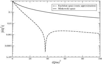
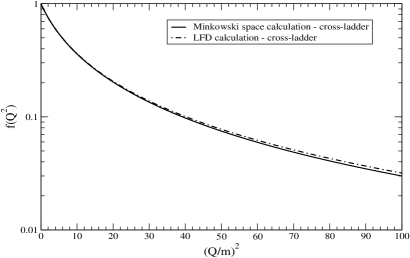
Figure 13: Left: Form factor via Minkowski BS amplitude (solid curve) and in static approximation (dashed).
Right: Form factor via Minkowski BS amplitude (solid curve, the same as at left panel) and in LFD (dot-dashed).

7 Conclusions

We presented a new method for obtaining the solutions of the Bethe-Salpeter equation in Minkowski space, both for two spinless bosons and for two fermions. It is based on a Nakanishi integral representation of the BS amplitude and on subsequent Light-Front projection.

The binding energies for these systems are calculated. They coincide with the ones found via Euclidean space solution, thus providing a validity test of our method. For two fermions, the solutions for the scalar exchange and positronium states without vertex form factor ($\Lambda\to\infty$) are stable below some critical value $g_{c}$ of the coupling constant, respectively $g_{c}=2\pi$ (scalar exchange) and $g_{c}=\pi$ (positronium).

The BS amplitudes are obtained in terms of the computed Nakanishi weight functions. They exhibit a singular behaviour due, on one hand, to the poles of the free propagators and, on the other hand, to non analytic branch cuts which are responsible for the appearance of an imaginary part.

Some applications to em form factors are also presented. We demonstrate that the Wick rotation in the variable $k_{0}$ – argument of the BS amplitude – is not allowed. It is prevented by the singularities which appear in the first quadrant of the complex $k_{0}$-plane and whose contributions are hardly evaluable in practice. Neglecting these contributions, one obtains an approximate expression which supposes the knowledge of Euclidean BS amplitude in a non-zero momentum frame. The latter requires to solve numerically a much more involved - though solvable - equation than at rest. On the contrary, in terms of the BS amplitude in Minkowski space, represented in the Nakanishi form (2), the form factors can be calculated without any problem.

Appendix A Numerical methods

The numerical methods wil be illustrated by considering the general case of $n_{a}$ coupled two-dimensional integral equations for the Nakanishi weight functions $g_{a}$ in the form:

$$\int_{0}^{\infty}d\gamma^{\prime}\;\int_{-1}^{+1}dz^{\prime}\;V^{g}_{a}(\gamma,z,\gamma^{\prime},z^{\prime})\;g_{a}(\gamma^{\prime},z^{\prime})=\sum_{a,a^{\prime}=1}^{n_{a}}\int_{0}^{\infty}d\gamma^{\prime}\;\int_{-1}^{+1}dz^{\prime}\;V^{d}_{aa^{\prime}}(\gamma,z,\gamma^{\prime},z^{\prime})\;g_{a^{\prime}}(\gamma^{\prime},z^{\prime})$$ (25)

For the scalar case the number of amplitudes is $n_{a}=1$ while for fermions it depends on the quantum numbers of the state ($n_{a}$=4 for $J=0$, $n_{a}=8$ for $J=1$).

Equation (25) has been solved by expanding the unknown functions $g_{a}$ on a bicubic spline basis [21] over a compact integration domain $\Omega=I_{\gamma}\times I_{z}=[0,\gamma_{max}]\times[-1,+1]$:

$$g_{a}(\gamma,z)=\sum_{i=0}^{2N_{\gamma}+1}\sum_{j=0}^{2N_{z}+1}g_{aij}S_{i}(\gamma)S_{j}(z)\qquad\forall(\gamma,z)\in\Omega$$ (26)

The interval $I_{x}$ corresponding to variable $x=\gamma,z$ is divided into $N_{x}$ subintervals – $[x_{i},x_{i+1}]$ with $i=0,\ldots N_{x}$ – satisfying $x_{0}=x_{min}$ and $x_{N_{x}}=x_{max}$. The distribution of grid points $G_{x}=\{x_{i}\}$ are adjusted to the structure of the solution. By means of expansion (26), equation (25) can be written in the form

$$\sum_{a^{\prime}i^{\prime}j^{\prime}}B_{a^{\prime}i^{\prime}j^{\prime}}(\gamma,z)g_{a^{\prime}i^{\prime}j^{\prime}}=\sum_{a^{\prime}i^{\prime}j^{\prime}}A_{a^{\prime}i^{\prime}j^{\prime}}(\gamma,z)g_{a^{\prime}i^{\prime}j^{\prime}}$$ (27)

with

$$B_{a^{\prime}i^{\prime}j^{\prime}}(\gamma,z) = \int_{0}^{\infty}d\gamma^{\prime}\int_{-1}^{+1}dz^{\prime}\;V^{g}_{a}(\gamma,z,\gamma^{\prime},z^{\prime})\;S_{i^{\prime}}(\gamma^{\prime})S_{j^{\prime}}(z^{\prime})\;\delta_{aa^{\prime}}$$ (28)

$$A_{a^{\prime}i^{\prime}j^{\prime}}(\gamma,z) = \int_{0}^{\infty}d\gamma^{\prime}\int_{-1}^{+1}dz^{\prime}\;V^{d}_{aa^{\prime}}(\gamma,z,\gamma^{\prime},z^{\prime})\;S_{i^{\prime}}(\gamma^{\prime})S_{j^{\prime}}(z^{\prime})$$ (29)

The left hand side of (27) is in fact diagonal in the number of amplitudes.

The spline functions for the expansion on a variable $x$, $S_{j}(x)$, are defined once the corresponding grid points $G_{x}=\{x_{0},x_{1},\ldots,x_{N_{x}}\}$ are fixed. These are $2N_{x}+1$ functions, usually denoted by $S_{0},S_{1},\ldots S_{2N_{x}+1}$.

The functions $S_{2i}$ and $S_{2i+1}$ are associated to the grid point $x_{i}$ and have a support limited to the two consecutive intervals surrounding it, i.e. $[x_{i-1},x_{i+1}]$, a property that makes easier the computation of integrals (28) and (29). Their analytic expressions are given by

$$S_{2i}(x) = \left\{\begin{array}[]{ll}3\left(\frac{x-x_{i-1}}{x_{i}-x_{i-1}}\right)^{2}-2\left(\frac{x-x_{i-1}}{x_{i}-x_{i-1}}\right)^{3}&{\rm if}\;x\in\left[x_{i-1},x_{i}\right]\\ 3\left(\frac{x_{i+1}-x}{x_{i+1}-x_{i}}\right)^{2}-2\left(\frac{x_{i+1}-x}{x_{i+1}-x_{i}}\right)^{3}&{\rm if}\;x\in\left[x_{i},x_{i+1}\right]\\ 0&{\rm if}\;x\notin\left[x_{i-1},x_{i+1}\right]\end{array}\right.$$

$$S_{2i+1}(x) = \left\{\begin{array}[]{ll}\left[-\left(\frac{x-x_{i-1}}{x_{i}-x_{i-1}}\right)^{2}+\left(\frac{x-x_{i-1}}{x_{i}-x_{i-1}}\right)^{3}\right](x_{i}-x_{i-1})&{\rm if}\;x\in\left[x_{i-1},x_{i}\right]\\ \left[+\left(\frac{x_{i+1}-x}{x_{i+1}-x_{i}}\right)^{2}-\left(\frac{x_{i+1}-x}{x_{i+1}-x_{i}}\right)^{3}\right](x_{i+1}-x_{i})&{\rm if}\;x\in\left[x_{i},x_{i+1}\right]\cr 0&{\rm if}\;x\notin\left[x_{i-1},x_{i+1}\right]\end{array}\right.$$

and they are such that the values of the solutions at the grid points are simply given by the even coefficients of the expansion (26), i.e. :

$$g_{a}(\gamma_{i},z_{j})=g_{a,2i,2j}$$ (32)

They are represented in figure 14.

Figure 14. Cubic spline functions associated to the grid point $x_{i}$.

Equation (27) is validated on a ensemble $\{\bar{\gamma}_{i},\bar{z}_{j}\}\subset\Omega$ of $(2N_{\gamma}+2)(2N_{z}+2)$ ”collocation” points which are taken equal to the N=2 Gauss quadrature abcises inside each subinterval of $I_{x}$ plus the 2 borders. This leads to a generalized eigenvalue problem

$$\lambda\;B(M)g=A(M)g$$ (33)

in which matrices $B$ and $A$ represent respectively the integral operators of the left- and right-hand sides of (25) and have the matrix elements

$$B_{aij,a^{\prime}i^{\prime}j^{\prime}} = B_{a^{\prime}i^{\prime}j^{\prime}}(\bar{\gamma}_{i},\bar{z}_{j})$$

$$A_{aij,a^{\prime}i^{\prime}j^{\prime}} = A_{a^{\prime}i^{\prime}j^{\prime}}(\ \bar{\gamma}_{i},\bar{z}_{j})$$

The unknown coefficients $g_{aij}$ are determined by the solutions of (33) corresponding to $\lambda(M)=1$.

Notice that the value of the solutions at the collocation points are given by the matrix product

$$g_{a}(\bar{\gamma}_{i},\bar{z}_{j})=\sum_{i^{\prime}j^{\prime}}U_{ij,i^{\prime}j^{\prime}}\;g_{a^{\prime}i^{\prime}j^{\prime}}$$

with the spline matrix $U$ given by

$$U_{ij,i^{\prime}j^{\prime}}=S_{i^{\prime}}(\bar{\gamma}_{i},)S_{j^{\prime}}(\bar{z}_{j})$$

It turns out that the discretized integral operator $B$ has very small eigenvalues. They are unphysical but make unstable the solution of the system (33). To regularize $B$, we have added a small constant $\varepsilon_{R}$ to its diagonal part on the form:

$$B\to B+\varepsilon_{R}\;U$$ (34)

This procedure allows us to obtain stable eigenvalues with an accuracy of the same order than $\varepsilon_{R}$ until values of $\varepsilon_{R}$ as small as $10^{-12}$.

The property (32) is very useful to implement boundary conditions to the solutions we are interested in. Although not necessary when working in momentum space integral equations, it uses to help the convergence of the numerical algorithms and allows to avoid unwanted solutions, which can be either due to the discretisation on a finite box or having other kind of symmetries. If we know in advance, for instance, that the solution vanishes at $z=\pm 1$, this implies according to (32) to impose to the coefficients $g_{a,i,0}\equiv g_{a,i,2N}\equiv 0$, that is in practice to remove them from the expansion (26) with the consequent reduction in the dimension of the matrix equation (33).

References

- [1] Salpeter, E.E., Bethe, H.A.: A Relativistic Equation for Bound-State Problems. Phys. Rev. 84, 1232 (1951)
- [2] Wick, G.C.: Properties of Bethe-Salpeter Wave Functions. Phys. Rev. 96, 1124 (1954)
- [3] Nakanishi, N.: A General Survey of the Theory of the Bethe-Salpeter Equation. Prog. Theor. Phys. Suppl. 43, 1 (1969)
- [4] Nakanishi, N.: Behavior of the Solutions to the Bethe-Salpeter Equation. Prog. Theor. Phys. Suppl. 95, 1 (1988)
- [5] Nieuwenhuis, T., Tjon, J.A.: O(4) Expansion of the Ladder Bethe-Salpeter Equation. Few-Body Syst. 21, 167 (1996)
- [6] Efimov, G.V.: On the Ladder Bethe-Salpeter Equation. Few-Body Syst., 33, 199 (2003)
- [7] Kusaka, K., Williams, A.G.: Solving the Bethe-Salpeter equation for scalar theories in Minkowski space. Phys. Rev. D 51, 7026 (1995)
- [8] Kusaka, K., Simpson, K., Williams, A.G.: Solving the Bethe-Salpeter equation for bound states of scalar theories in Minkowski space. Phys. Rev. D 56, 5071 (1997)
- [9] Nakanishi, N.: Partial-Wave Bethe-Salpeter Equation. Phys. Rev. 130, 1230 (1963)
- [10] Nakanishi, N.: Graph Theory and Feynman Integrals. (Gordon and Breach, New York, 1971)
- [11] Sauli, V., Adam, J. Jr.: Study of relativistic bound states for scalar theories in Bethe-Salpeter and Dyson-Schwinger formalism. Phys. Rev. D 67, 085007 (2003)
- [12] Sauli, V.: Solving the Bethe-Salpeter equation for a pseudoscalar meson in Minkowski space. J. Phys. G 35, 035005 (2008); arXiv:0802.2955(hep-ph)
- [13] Bondarenko, S.G., Burov, V.V., Molochkov, A.M. Smirnov, G.I., Toki, H.: Bethe-Salpeter approach with the separable interaction for the deuteron. Prog. in Part. and Nucl. Phys., 48, 449 (2002)
- [14] Bondarenko, S.G., Burov, V.V., Pauchy Hwang, W.-Y., Rogochaya, E.P.: Relativistic multirank interaction kernels of the neutron-proton system. Nucl. Phys. A 832, 233 (2010); arXiv:0810.4470 (nucl-th); arXiv:1002.0487 (nucl-th)
- [15] Karmanov, V.A., Carbonell, J.: Solving Bethe-Salpeter equation in Minkowski space. Eur. Phys. J. A 27, 1 (2006); hep-th/0505261
- [16] Carbonell, J., Karmanov, V.A.: Solving Bethe-Salpeter equation for two fermions in Minkowski space. Eur. Phys. J. A 46, 387 (2010); arXiv:1010.4640(hep-ph)
- [17] Cutkosky, R.E.: Solutions of a Bethe-Salpeter Equation. Phys. Rev. 96, 1135 (1954)
- [18] Carbonell, J., Karmanov, V.A.: Cross-ladder effects in Bethe-Salpeter and Light-Front equations. Eur. Phys. J. A 27, 11 (2006); hep-th/0505262
- [19] Carbonell, J., Desplanques, B., Karmanov, V.A., Mathiot, J.-F.: Explicitly Covariant Light-Front Dynamics and Relativistic Few-Body Systems. Phys. Reports, 300 215 (1998)
- [20] Mangin-Brinet, M., Carbonell, J.: Solutions of the Wick-Cutkosky model in the light front dynamics. Phys. Lett. B, 474, 237 (2000)
- [21] Payne, G.L.: Models and Methods in Few-Body Physics. Edited by L.S. Ferreira et al., Lect. Notes in Phys. (Springer Berlin), 93, 64 (1987)
- [22] Nieuwenhuis, T., Tjon, J.A.: Nonperturbative Study of Generalized Ladder Graphs in a Theory. Phys. Rev. Lett. 77, 814 (1996)
- [23] Levine, M.J., Wright, J.: Comment on Nonplanar Graphs and the Bethe-Salpeter Equation. Phys. Rev. D 2, 2509 (1970)
- [24] Cooke, J.R., Miller, G.A.: Ground states of the Wick-Cutkosky (scalar Yukawa) model using light-front dynamics. Phys. Rev. C 62, 054008 (2000)
- [25] Cooke, J.R., Miller, G.A., Phillips, D.R.: Restoration of rotational invariance of bound states on the light front. Phys. Rev. C 61, 064005 (2000)
- [26] Amghar, A., Desplanques, B., Theusl, L.: From the Bethe Salpeter equation to nonrelativistic approaches with effective two-body interactions. Nucl. Phys. A 694, 439 (2001)
- [27] Ji, C.-R.: The self-energy corrections to the light-cone two-body equation in -theories. Phys. Lett. B 322, 389 (1994)
- [28] Ji, C.-R., Kim, G.-H., Min, D.-P.: Self-energy effect on the rotation symmetry in the light-cone-quantized scalar field scattering. Phys. Rev. D 51, 879 (1995)
- [29] Schoonderwoerd, N.C.J., Bakker, B.L.G., Karmanov, V.A.: Entanglement of Fock-space expansion and covariance in light-front Hamiltonian dynamics. Phys. Rev. C 58, 3093 (1998)
- [30] Hwang, D.S., Karmanov, V.A.: Many-body Fock sectors in Wick-Cutkosky model. Nucl. Phys. B 696, 413 (2004)
- [31] Karmanov, V.A., Carbonell, J.: Bethe-Salpeter equation in Minkowski space with cross-ladder kernel. Nucl. Phys. B (Proc.Suppl.) 161, 123 (2006); nucl-th/0510051
- [32] Dorkin, S.M., Beyer, M., Semykh, S.S., Kaptari, L.P.: Two-fermion bound states within the Bethe-Salpeter approach. Few-Body Syst. 42, 1 (2008); arXiv:0708.2146 (nucl-th)
- [33] Mangin-Brinet, M., Carbonell, J., Karmanov, V.A.: Two-fermion relativistic bound states in Light-Front Dynamics. Phys. Rev. C 68, 055203 (2003)
- [34] Mangin-Brinet, M., Carbonell, J., Karmanov, V.A.: Stability of bound states in the light-front Yukawa model. Phys. Rev. D 64, 027701 (2001)
- [35] Mangin-Brinet, M., Carbonell, J., Karmanov, V.A.: Relativistic bound states in Yukawa model. Phys. Rev. D 64, 125005 (2001)
- [36] Zuilhof, M.J., Tjon, J.A.: Electromagnetic properties of the deuteron and the Bethe-Salpeter equation with one-boson exchange. Phys. Rev. C 22, 2369 (1980)
- [37] Carbonell, J., Karmanov, V.A., Mangin-Brinet, M.: Electromagnetic form factor via Bethe-Salpeter amplitude in Minkowski space. Eur. Phys. J. A 39, 53 (2009); arXiv:0809.3678 (hep-th)
- [38] Karmanov, V.A., Carbonell, J., Mangin-Brinet, M.: Electromagnetic form factor via Minkowski and Euclidean Bethe-Salpeter amplitudes. Few-Body Syst., 44, 283 (2008); arXiv:0712.0971(hep-th)
- [39] Maris, P., Tandy, P.C.: QCD modeling of hadron physics. Nucl. Phys. B (Proc. Suppl.) 161, 136 (2006); arXiv:nucl-th/0511017
- [40] Bhagwat, M.S., Maris, P.: Vector meson form factors and their quark-mass dependence. Phys. Rev. C 77, 025203 (2008); arXiv:nucl-th/0612069