Preface

The series of workshops on ”What Comes Beyond the Standard Models?” started in 1998 with the idea of Norma and Holger for organizing a real workshop, in which participants would spend most of the time in discussions, confronting different approaches and ideas. The picturesque town of Bled by the lake of the same name, surrounded by beautiful mountains and offering pleasant walks and mountaineering, was chosen to stimulate the discussions. The workshops take place in the house gifted to the Society of Mathematicians, Physicists and Astronomers of Slovenia by the Slovenian mathematician Josip Plemelj, well known to the participants by his work in complex algebra.

The idea was successful and has developed into an annual workshop, which is taking place every year since 1998. This year the thirteenth workshop took place. Very open-minded and fruitful discussions have become the trade-mark of our workshop, producing several new ideas and clarifying the proposed ones. The first versions of published works appeared in the proceedings to the workshop.

In this thirteenth workshop, which took place from $12^{th}$ to $22^{nd}$ of July 2010, we were discussing several topics, most of them presented in this Proceedings and in the discussion section.

One of the main topics was this time the ”approach unifying spin and charges and predicting families” (the spin-charge-family-theory shortly), as the new way beyond the standard model of the electroweak and colour interactions, accompanied by the critical discussions about all the traps, which the theory does and might in future confront, before being accepted as a theory which answers the open questions which the standard model leaves unanswered. Proposing the mechanism for generating families, this theory is predicting the fourth family which is waiting to be observed and the stable fifth family which have a chance to form the dark matter. There were discussions of the questions like: To which extent can the spin-charge-family-theory answer the open questions of both standard models – the elementary particle one and the cosmological one? Are the clusters of the fifth family members alone what constitute the dark matter? Can the fifth family baryons and neutrinos explain the observed properties of the dark matter with the direct measurements included? How do fermions and gauge bosons of this theory behave in phase transitions, through which the primordial plasma went? How do very heavy fifth family neutrinos and colourless fifth family baryons behave in the electroweak phase transitions? How do (very heavy) fifth family quarks behave in the colour phase transition? Why does the colour phase transition occur at $\approx 1$ GeV? What does trigger the fermion-antifermion asymmetry in this theory and how does the existence of two stable families influences the matter-antimatter asymmetry? Although the theory predicts the mass matrices, it also connects strongly the mass matrix properties of the members of families on the tree level. Does the coherent contribution of fields beyond the tree level explains the great difference in masses and mixing matrices among the (so far measured) families? Can a complex action function as a cutoff in loop diagrams?

We discuss the model with the complex action and its application to the presently observed properties of fermions and bosons as well as about the possibility that this model would lead to improvement in the sense of interpretation of quantum mechanic, since it includes the DeBroglie-Bohm-particle approach to quantum mechanics.

We discuss also the dark matter direct measurements and possible explanations of the experimental data, if a very heavy stable family, as the fifth family is, constitutes the dark matter as neutral baryons and neutrinos or as neutral nuclei (both with respect to the colour and electromagnetic charge). There were also the talk and discussions afterwards about what signals from the dark matter are expected to be seen at the LHC .

Talks and discussions in our workshop are not at all talks in the usual way. Each talk or discussions lasted several hours, divided in two hours blocks, with a lot of questions, explanations, trials to agree or disagree from the audience or a speaker side. Most of talks are ”unusual” in the sense that they are trying to find out new ways of understanding and describing the observed phenomena. Although we always hope that the progress made in discussions will reflect in the same year proceedings, it happened many a time that the topics appear in the next or after the next year proceedings. This is happening also in this year. There fore neither the discussion section nor the talks published in this proceedings, manifest all the discussions and the work done in this workshop.

Several teleconferences were taking place during the Workshop on various topics. It was organized by the Virtual Institute for Astrophysics
(wwww.cosmovia.org) of Maxim with able support by Didier Rouable. We managed to have ample discussions and we thank all the participants, those presenting a talk and those contributing in discussions. The reader can find the talks delivered by John Ellis, N.S. Mankoč Borštnik and H.B. Nielsen on www.cosmovia.org,
http://viavca.in2p3.fr/what_comes_beyond_the_standard_models_xiii.html
Let us thanks cordially all the participants, those present really and those present virtually, for their presentations and in particular for really fruitful discussions and the good working atmosphere.

Norma Mankoč Borštnik, Holger Bech Nielsen, Maxim Y. Khlopov,
(the Organizing comittee)
Norma Mankoč Borštnik, Holger Bech Nielsen, Dragan Lukman,

(the Editors)

Ljubljana, December 2010

Predgovor (Preface in Slovenian Language)

A. Ali Khan¹ and H. Markum² Thanks to the organizers of the Workshop 2010 ’What Comes Beyond the Standard Models’ in BledUniversidad de Zacatecas
Ap. Postal 636, Suc. 3 Cruces, C. P. 98062
Zacatecas, Zac., MéxicoUniversidad de Zacatecas, A. P. 636, Suc. 3 Cruces
Zacatecas, Zac. 98062, México
E-mail: valeri@fisica.uaz.edu.mx
http://fisica.uaz.edu.mx/~valeriTheory Division, CERN, CH–1211 Genève 23, Switzerland;
Theoretical Physics and Cosmology Group, Department of Physics, King’s College London, London WC2R 2LS, UK
    
CERN-PH-TH/2010-258                    KCL-PH-TH/2010-31
      Department of Physics,
İzmir Institute of Technology
Gülbahçe Köyü, Urla, İzmir 35430, TurkeyDepartamento de Física, Escuela Superior de Física y Matemáticas, I.P.N.,
U. P. ”Adolfo López Mateos”. C. P. 07738, México, D.F., México.¹National Research Nuclear University ”Moscow Engineering Physics Institute”, 115409 Moscow, Russia
² Centre for Cosmoparticle Physics ”Cosmion” 115409 Moscow, Russia
³ APC laboratory 10, rue Alice Domon et Léonie Duquet
75205 Paris Cedex 13, FranceDepartment of Physics, FMF, University of Ljubljana,
Jadranska 19, SI-1000 Ljubljana, SloveniaDepartment of Physics, FMF, University of Ljubljana,
Jadranska 19, SI-1000 Ljubljana, SloveniaLaboratoire de Physique Théorique & Astroparticules
Université Montpellier 2, CNRS/IN2P3, Montpellier, France
gilbert.moultaka@univ-montp2.fr¹The Niels Bohr Institute, University of Copenhagen,
Copenhagen $\phi$, DK2100, Denmark
²Okayama Institute for Quantum Physics,
Kyoyama 1, Okayama 700-0015, Japan
³Theoretical Physics Laboratory,
The Institute of Physics and Chemical Research (RIKEN),
Wako, Saitama 351-0198, Japan¹Department of Physics, FMF, University of Ljubljana, Jadranska 19, SI-1000 Ljubljana
²Physics Department, Columbia University, New York, New York 10027, USA¹Departamento de Física, Escuela Superior de Física y Matemáticas, I.P.N.,
U. P. ”Adolfo López Mateos”. C. P. 07738, México, D.F., México.
²Department of Physics, FMF, University of Ljubljana, Jadranska 19, SI-1000 Ljubljana, Slovenia¹Moscow Engineering Physics Institute (National Nuclear Research University), 115409 Moscow, Russia
²Centre for Cosmoparticle Physics ”Cosmion” 115409 Moscow, Russia
³APC laboratory 10, rue Alice Domon et Léonie Duquet
75205 Paris Cedex 13, France
⁴Department of Physics, FMF, University of Ljubljana,
Jadranska 19, SI-1000 Ljubljana¹National Research Nuclear University ”Moscow Engineering Physics Institute”, 115409 Moscow, Russia
² Centre for Cosmoparticle Physics ”Cosmion” 115409 Moscow, Russia
³ APC laboratory 10, rue Alice Domon et Léonie Duquet
75205 Paris Cedex 13, France¹Department of Physics, FMF, University of Ljubljana,
Jadranska 19, SI-1000 Ljubljana, Slovenia
²Department of Physics, Niels Bohr Institute, Blegdamsvej 17,
Copenhagen, DK-2100¹Faculty of Mathematics and Physics, University of Ljubljana, Jadranska 19, P.O. Box 2964, 1001 Ljubljana, Slovenia
²J. Stefan Institute, 1000 Ljubljana, Slovenia¹The Niels Bohr Institute, Copenhagen, Denmark
hbech@nbi.dk
²University of Ljubljana, jadranska 19, 1000 Ljubljana, Slovenia
norma.mankoc@fmf.uni-lj.si
³The Niels Bohr Institute, Copenhagen, Denmark
⁴University of Montpellier II, 34095 Montpellier, cedex 5, France
gilbert.moultaka@lpta.univ-montp2.fr14U
155 E 34 Street
New York, NY 10016 ¹Moscow Engineering Physics Institute (National Nuclear Research University), 115409 Moscow, Russia
²Centre for Cosmoparticle Physics ”Cosmion” 125047 Moscow, Russia
³APC laboratory 10, rue Alice Domon et Léonie Duquet
75205 Paris Cedex 13, France

Serija delavnic ”Kako preseči oba standardna modela, kozmološkega in elektrošibkega” (”What Comes Beyond the Standard Models?”) se je začela leta 1998 z idejo, da bi organizirali delavnice, v katerih bi udeleženci posvetili veliko časa diskusijam, ki bi kritično soočile različne ideje in teorije. Mesto Bled ob slikovitem jezeru je za take delavnice zelo primerno, ker prijetni sprehodi in pohodi na čudovite gore, ki kipijo nad mestom, ponujajo priložnosti in vzpodbudo za diskusije. Delavnica poteka v hiši, ki jo je Društvu matematikov, fizikov in astronomov Slovenije zapustil v last slovenski matematik Josip Plemelj, udeležencem delavnic, ki prihajajo iz različnih koncev sveta, dobro poznan po svojem delu v kompleksni algebri.

Ideja je zaživela, rodila se je serija letnih delavnic, ki potekajo vsako leto od 1998 naprej. To leto je potekala trinajstič. Zelo odprte in plodne diskusije so postale značilnost naših delavnic, porodile so marsikatero novo idejo in pomagale razjasniti in narediti naslednji korak predlaganim idejam in teorijam. Povzetki prvih novih korakov in dognanj so izšle v zbornikih delavnic.

Na letošnji, trinajsti, delavnici, ki je potekala od 12. do 22. malega srpana (julija) 2010, smo razpravljali o več temah, večina je predstavljena v tem zborniku.

Ena od osnovnih tem je bila tokrat ”teorija enotnih spinov in nabojev, ki napoveduje družine” (na kratko: teorija spina-nabojev-družin) kot novo pot za razširitev standardnega modela elektrošibke in barvne interakcije. Spremljale so jo kritične razprave o pasteh, s katerimi se ta teorija sooča in se bo soočala v prihodnje, preden bo lahko sprejeta kot odgovor na odprta vprašanja standardnega modela. Teorija predlaga mehanizem za nastanek družin, napoveduje četrto družino, ki jo utegnejo opaziti, in peto družino, iz katere bi utegnila biti temna snov. Razpravljali smo o vprašanjih kot so: V kolikšni meri lahko teorija spina-nabojev-družin odgovori na odprta vprašanja obeh standardnih modelov – standardnega modela za osnovne delce in polja in standardnega kozmološkega modela? Ali so gruče iz članov pete družine edina sestavina temne snovi? Ali lahko barioni in nevtrini pete družine pojasnijo opažene lastnosti temne snovi, vključno z direktnimi meritvami? Kako se fermioni in umeritvena polja te teorije obnašajo pri faznih prehodih, skozi katere je šla prvotna plazma? Kako se zelo težki nevtrini in brezbarvni barioni pete družine obnašajo pri elektrošibkih faznih prehodih? Kako se obnašajo (zelo težki) kvarki pete družine pri barvnem faznem prehodu? Zakaj se barvni fazni prehod zgodi pri $\approx 1$ GeV? Kaj v tej teoriji sproži asimetrijo fermionov in antifermionov in kako obstoj dveh stabilnih družin vpliva na asimetrijo snov-antisnov? Čeprav teorija napove masne matrike, obenem krepko poveže lastnosti masnih matrik članov družin na drevesnem nivoju. Ali koherentni prispevek polj pod drevesnim nivojem pojasni velike razlike v masah in mešalnih matrikah med (že izmerjenimi) družinami? Ali lahko kompleksna akcija učinkuje kot zgornja meja v diagramih zank?

Razpravljali smo o modelu s kompleksno akcijo in o možnosti, da kompleksna akcija pojasni nekatere lastnosti fermionov in bozonov, denimo skalo elektrošibkega prehoda pri 200 GeV, pa tudi o izbolšani interpretacijo kvantne mehanike, ker vključuje DeBroglie-Bohmov pristop k kvantni mehaniki.

Veliko časa smo posvetili direktnim meritvam temne snovi in možnim razlagam doslej zbranih podatkov, če gradi temno snov težka stabilna družina kvarkov in leptonov, denimo peta družina. Je temna snov iz nevtralnih barionov (nevtralnih glede na barvni in elektromagnetni naboj) in nevtrinov ali iz elektromagnetno nevtralnih jeder, ki jih sestavljajo barvno nevtralni težki barioni in brezbarvni barioni prve družine.

Imeli smo predavanje in nato živahno diskusijo o tem, kakšne signale temne snovi lahko pričakujemo na pospeševalniku LHC.

Predavanja in razprave na naši delavnici niso predavanja v običajnem smislu. Vsako predavanje ali razprava je trajala več ur, razdelejnih na bloke po dve uri, z veliko vprašanji, pojasnili, poskusi, da bi predavatelj in občinstvo razumeli trditve, kritike in se na koncu strinjali ali pa tudi ne. Večina predavanj je ’neobičajnih’ v tem smislu, da poskušajo najti nove matematične načine opisa, pa tudi razumevanja doslej opaženih pojavov. Čeprav vedno upamo, da bomo vsako leto uspeli zapisati vsa nova dognanja, nastala v ali ob diskusijah, se vseeno mnogokrat zgodi, da se prvi zapisi o napredku pojavijo šele v kasnejših zbornikh. Tako tudi letošnji zbornik ne vsebuje povzetkov vseh uspešnih razprav ter napredka pri temah, predstavljenih v predavanjih.

Med delavnico smo imeli več spletnih konferenc na različne teme. Organiziral jih je Virtualni institut za astrofiziko iz Pariza (www.cosmovia.org, vodi ga Maxim) ob spretni podpori Didierja Rouablea. Uspelo nam je odprto diskutirati kar z nekaj laboratoriji po svetu. Toplo se zahvaljujemo vsem udeležencem, tako tistim, ki so imeli predavanje, kot tistim, ki so sodelovali v razpravi, na Bledu ali preko spleta. Bralec lahko najde posnetke predavanj, ki so jih imeli John Ellis, N.S. Mankoč Borštnik in H.B. Nielsen na spletni povezavi
http://viavca.in2p3.fr/what_comes_beyond_the_standard_models_xiii.html
Prisrčno se zahvaljujemo vsem udeležencem, ki so bili prisotni, tako fizično kot virtualno, za njihova predavanja, za zelo plodne razprave in za delovno vzdušje.

Norma Mankoč Borštnik, Holger Bech Nielsen, Maxim Y. Khlopov,
(Organizacijski odbor)
Norma Mankoč Borštnik, Holger Bech Nielsen, Dragan Lukman,

(uredniki)

Ljubljana, grudna (decembra) 2010

Talk Section
All talk contributions are arranged alphabetically with respect to the first author’s name.

Noncommutativity and Topology within Lattice Field Theories

A. Ali Khan¹ and H. Markum² Thanks to the organizers of the Workshop 2010 ’What Comes Beyond the Standard Models’ in BledUniversidad de Zacatecas
Ap. Postal 636, Suc. 3 Cruces, C. P. 98062
Zacatecas, Zac., MéxicoUniversidad de Zacatecas, A. P. 636, Suc. 3 Cruces
Zacatecas, Zac. 98062, México
E-mail: valeri@fisica.uaz.edu.mx
http://fisica.uaz.edu.mx/~valeriTheory Division, CERN, CH–1211 Genève 23, Switzerland;
Theoretical Physics and Cosmology Group, Department of Physics, King’s College London, London WC2R 2LS, UK
    
CERN-PH-TH/2010-258                    KCL-PH-TH/2010-31
      Department of Physics,
İzmir Institute of Technology
Gülbahçe Köyü, Urla, İzmir 35430, TurkeyDepartamento de Física, Escuela Superior de Física y Matemáticas, I.P.N.,
U. P. ”Adolfo López Mateos”. C. P. 07738, México, D.F., México.¹National Research Nuclear University ”Moscow Engineering Physics Institute”, 115409 Moscow, Russia
² Centre for Cosmoparticle Physics ”Cosmion” 115409 Moscow, Russia
³ APC laboratory 10, rue Alice Domon et Léonie Duquet
75205 Paris Cedex 13, FranceDepartment of Physics, FMF, University of Ljubljana,
Jadranska 19, SI-1000 Ljubljana, SloveniaDepartment of Physics, FMF, University of Ljubljana,
Jadranska 19, SI-1000 Ljubljana, SloveniaLaboratoire de Physique Théorique & Astroparticules
Université Montpellier 2, CNRS/IN2P3, Montpellier, France
gilbert.moultaka@univ-montp2.fr¹The Niels Bohr Institute, University of Copenhagen,
Copenhagen $\phi$, DK2100, Denmark
²Okayama Institute for Quantum Physics,
Kyoyama 1, Okayama 700-0015, Japan
³Theoretical Physics Laboratory,
The Institute of Physics and Chemical Research (RIKEN),
Wako, Saitama 351-0198, Japan¹Department of Physics, FMF, University of Ljubljana, Jadranska 19, SI-1000 Ljubljana
²Physics Department, Columbia University, New York, New York 10027, USA¹Departamento de Física, Escuela Superior de Física y Matemáticas, I.P.N.,
U. P. ”Adolfo López Mateos”. C. P. 07738, México, D.F., México.
²Department of Physics, FMF, University of Ljubljana, Jadranska 19, SI-1000 Ljubljana, Slovenia¹Moscow Engineering Physics Institute (National Nuclear Research University), 115409 Moscow, Russia
²Centre for Cosmoparticle Physics ”Cosmion” 115409 Moscow, Russia
³APC laboratory 10, rue Alice Domon et Léonie Duquet
75205 Paris Cedex 13, France
⁴Department of Physics, FMF, University of Ljubljana,
Jadranska 19, SI-1000 Ljubljana¹National Research Nuclear University ”Moscow Engineering Physics Institute”, 115409 Moscow, Russia
² Centre for Cosmoparticle Physics ”Cosmion” 115409 Moscow, Russia
³ APC laboratory 10, rue Alice Domon et Léonie Duquet
75205 Paris Cedex 13, France¹Department of Physics, FMF, University of Ljubljana,
Jadranska 19, SI-1000 Ljubljana, Slovenia
²Department of Physics, Niels Bohr Institute, Blegdamsvej 17,
Copenhagen, DK-2100¹Faculty of Mathematics and Physics, University of Ljubljana, Jadranska 19, P.O. Box 2964, 1001 Ljubljana, Slovenia
²J. Stefan Institute, 1000 Ljubljana, Slovenia¹The Niels Bohr Institute, Copenhagen, Denmark
hbech@nbi.dk
²University of Ljubljana, jadranska 19, 1000 Ljubljana, Slovenia
norma.mankoc@fmf.uni-lj.si
³The Niels Bohr Institute, Copenhagen, Denmark
⁴University of Montpellier II, 34095 Montpellier, cedex 5, France
gilbert.moultaka@lpta.univ-montp2.fr14U
155 E 34 Street
New York, NY 10016 ¹Moscow Engineering Physics Institute (National Nuclear Research University), 115409 Moscow, Russia
²Centre for Cosmoparticle Physics ”Cosmion” 125047 Moscow, Russia
³APC laboratory 10, rue Alice Domon et Léonie Duquet
75205 Paris Cedex 13, France

Abstract

Theories with noncommutative space-time coordinates represent alternative candidates of grand unified theories. We discuss U(1) gauge theory in 2 and 4 dimensions on a lattice with N sites. The mapping to a U(N) plaquette model in the sense of Eguchi and Kawai can be used for computer simulations. In 2D it turns out that the formulation of the topological charge leads to the imaginary part of the plaquette. Concerning 4D, the definition of instantons seems straightforward. One can transcribe the plaquette and hypercube formulation to the matrix theory. The transcription of a monopole observable seems to be difficult. The analogy to commutative U(1) theory of summing up the phases over an elementary cube does not obviously transfer to the U(N) theory in the matrix model. It would be interesting to measure the topological charge on a noncommutative hypercube. It would even be more interesting to find arguments and evidence for realization of noncommutative space-time in nature.

Abstract

We draw attention to some tune problems in constructions of the quantum-field operators for spins 1/2 and 1. They are related to the existence of negative-energy and acausal solutions of relativistic wave equations. Particular attention is paid to the chiral theories, and to the method of the Lorentz boosts.

Abstract

We proceed to derive equations for the symmetric tensor of the second rank on the basis of the Bargmann-Wigner formalism in a straightforward way. The symmetric multispinor of the fourth rank is used. It is constructed out of the Dirac 4-spinors. Due to serious problems with the interpretation of the results obtained on using the standard procedure we generalize it and obtain the spin-2 relativistic equations, which are consistent with those given before. The importance of the 4-vector field (and its gauge part) is pointed out.

Abstract

The prospects for detecting a candidate supersymmetric dark matter particle at the LHC are reviewed, and compared with the prospects for direct and indirect searches for astrophysical dark matter, on the basis of a frequentist analysis of the preferred regions of the Minimal supersymmetric extension of the Standard Model with universal soft supersymmetry breaking (the CMSSM) and a model with equal but non-universal supersymmetry-breaking contributions to the Higgs masses (the NUHM1). LHC searches may have good chances to observe supersymmetry in the near future - and so may direct searches for astrophysical dark matter particles.

Abstract

The metric reversal symmetry was introduced in the context of cosmological constant problem. Besides proposing a solution to the cosmological constant problem the metric reversal symmetry has also provided a framework for solution of the zero-point energy problem, an automatic Pauli-Villars-like regularization, and an interesting Kaluza-Klein spectrum with interesting phenomenological implications. In this talk I give a brief overall summary and discussion of these topics with their potential implications.

Abstract

I report new results on the study of fermion masses and quark mixing within a $SU(3)$ flavor symmetry model, where ordinary heavy fermions, top and bottom quarks and tau lepton become massive at tree level from Dirac See-saw mechanisms implemented by a new heavy family of $SU(2)_{L}$ weak singlet vector-like fermions, while light fermions get masses from one loop radiative corrections mediated by the massive $SU(3)$ gauge bosons. A recent quantitative analysis shows the existence of a low energy space parameter which is able to accommodate the quark and charged lepton masses as well as the quark mixing angle $(V_{CKM})_{12}=0.2253$ with the gauge boson masses in the TeV scale and a vector-like D quark of the order of $900\>GeV$. These predictions may be tested at the LHC. Furthermore, the above scenario enable us to suppress simultaneously the tree level $\Delta F=2$ processes for $K^{o}-\bar{K^{o}}$ and $D^{o}-\bar{D^{o}}$ meson mixing mediated by these extra horizontal gauge bosons within current experimental bounds.

Abstract

The nonbaryonic dark matter of the Universe is assumed to consist of new stable particles. A specific case is possible, when new stable particles bear ordinary electric charge and bind in heavy ”atoms” by ordinary Coulomb interaction. Such possibility is severely restricted by the constraints on anomalous isotopes of light elements that form positively charged heavy species with ordinary electrons. The trouble is avoided, if stable particles $X^{--}$ with charge -2 are in excess over their antiparticles (with charge +2) and there are no stable particles with charges +1 and -1. Then primordial helium, formed in Big Bang Nucleosynthesis, captures all $X^{--}$ in neutral ”atoms” of O-helium (OHe). Schrodinger equation for system of nucleus and OHe is considered and reduced to an equation of relative motion in a spherically symmetrical potential, formed by the Yukawa tail of nuclear scalar isoscalar attraction potential, acting on He beyond the nucleus, and dipole Coulomb repulsion between the nucleus and OHe at small distances between nuclear surfaces of He and nucleus. The values of coupling strength and mass of $\sigma$-meson, mediating scalar isoscalar nuclear potential, are rather uncertain. Within these uncertainties and in the approximation of rectangular potential wells and wall we find a range of these parameters, at which the sodium nuclei have a few keV binding energy with OHe. The result also strongly depend on the precise value of parameter $d_{o}$ that determines the size of nuclei. At nuclear parameters, reproducing DAMA results, OHe-nucleus bound states can exist only for intermediate nuclei, thus excluding direct comparison with these results in detectors, containing very light (e.g. ${}^{3}He$) and heavy nuclei (like Xe).

Abstract

This contribution is an attempt to try to understand the matter-antimatter asymmetry in the universe within the spin-charge-family-theory snmb2bnorma ; snmb2bpikanorma if assuming that transitions in non equilibrium processes among instanton vacua and complex phases in mixing matrices are the sources of the matter-antimatter asymmetry, as studied in the literature snmb2bgross ; snmb2brubakovshaposhnikov ; snmb2bdinekusenko ; snmb2btapeiling for several proposed theories. The spin-charge-family-theory is, namely, very promising in showing the right way beyond the standard model. It predicts families and their mass matrices, explaining the origin of the charges and of the gauge fields. It predicts that there are, after the universe passes through two $SU(2)\times U(1)$ phase transitions, in which the symmetry breaks from $SO(1,3)\times SU(2)\times SU(2)\times U(1)\times SU(3)$ first to $SO(1,3)\times SU(2)\times U(1)\times SU(3)$ and then to $SO(1,3)\times U(1)\times SU(3)$, twice decoupled four families. The upper four families gain masses in the first phase transition, while the second four families gain masses at the electroweak break. To these two breaks of symmetries the scalar non Abelian fields, the (superposition of the) gauge fields of the operators generating families, contribute. The lightest of the upper four families is stable (in comparison with the life of the universe) and is therefore a candidate for constituting the dark matter. The heaviest of the lower four families should be seen at the LHC or at somewhat higher energies.

Abstract

The theory unifying spin and charges and predicting families, proposed snmb3tgnorma ; snmb3tgpikanorma as a new way to explain the assumptions of the standard model of the electroweak and colour interactions, predicts at the low energy regime two (by the mixing matrices decoupled) groups of four families. All of them are massless before the two final breaks and identical with respect to the charges and spin. They differ only in the family quantum number. The fourth family of the lower group of four families (three of them known) is predicted to be possibly observed at the LHC or at somewhat higher energies and the stable of the higher four families – the fifth family – is the candidate to constitute the dark matter. In this paper the properties of the fields – spinors, gauge fields and scalar fields – before and after each of the two last successive breaks, leading to the (so far) observed quarks, leptons and gauge fields, are analysed as they follow from the spin-charge-family-theory.

Abstract

We give a short account of an old and somewhat unfashionable approach to quantum mechanics, arguing though for its potential to provide a new kind of Higgsless physics beyond the Standard Model.

Abstract

It is shown that the transactional interpretation of quantum mechanics being referred back to Feynman-Wheeler time reversal symmetric radiation theory is reminiscent of our complex action model. In our model the initial conditions are, in principle, even calculable. Thus the model philosophically points towards superdeterminism, but really the problem associated with Bell’s theorem is solved in our complex action model by removing the necessity for signals to travel faster than the speed of light for consistency.

As previously published our model predicts that the LHC (Large Hadron Collider) should have a failure before producing as many Higgs-particles as would have been produced by the SSC (Superconducting Super Collider) accelerator. In the present article, we point out that a card game to decide whether to restrict the operation of the LHC, which we proposed as means of testing our model will be a success under all circumstances.

Abstract

This discussion is to clarify what can be concluded from the so far analysed experimental data obtained in the XENON100 experiment blmbDAprile:2010um about the prediction of the ref. blmbDgn , which states: If the DAMA/LIBRA blmbDDAMA experiment measures the fifth family neutrons predicted by the ”spin-charge-family-theory” (of the author N.S. Mankoč Borštnik blmbDnorma ; blmbDpikanorma ; blmbDNF ) then new direct experiments will in a few years measure the fifth family neutrons as well.

Abstract

The approach unifying spin and charges and predicting families, proposed by N.S.M.B., predicts at the low energy regime two groups of four families, decoupled in the mixing matrix elements. To the mass matrices there are two kinds of contributions. One kind distinguishes on the tree level only among the members of one family, that is among the $u$-quark, $d$-quark, neutrino and electron, the left and right handed, while the other kind distinguishes only among the families. Beyond the tree level both kinds start to contribute coherently and it is expected that a detailed study of the properties of mass matrices beyond the tree level will explain a drastic difference in masses and mixing matrices between quarks and leptons. We report in this contribution on the analysis of one loop corrections to the tree level fermion masses and mixing matrices. The loop diagrams are mediated by gauge bosons and scalar fields.

Abstract

This discussion is to try to clarify whether the dark matter can be made out of the clusters of the members of the stable fifth family, which is predicted by the approach unifying spin and charges and predicting families proposed by Norma mksnmbDnorma ; mksnmbDpikanorma (to be named as the spin-charge-family-theory) in the scenario proposed by Maxim. Maxim’s scenario differs from the Norma’s one published in the ref. mksnmbDgn , in which Gregor and Norma evaluated that the fifth family members have the masses of around a few hundred TeV and that the current quark masses of the stable fifth family do not differ among themselves more than a few hundred GeV (see mksnmbDgn ; mksnmbDMN ). Then independently of the quark-antiquark fifth family asymmetry the fifth family neutrons and antineutrons constitute the dark matter, while the contribution of the fifth family neutrinos is negligible, provided that the fifth neutrino-antineutrino asymmetry is small enough. Maxim assumes for his scenario i. that the fifth family quarks are not heavier than a few TeV, ii. that there is an antiquark-quark asymmetry and iii. that $\bar{u}_{5}\bar{u}_{5}\bar{u}_{5}$ is the lightest baryon. If these three conditions are fulfilled Maxim mksnmbDMaxim found that the fifth family anti$u$-quark cluster with a charge $-2$ forming with the ordinary He nucleus an electromagnetically neutral object (Maxim calls it OHe) might be what constitute the dark matter. These two scenarios are discussed in this contribution.

Abstract

Positive results of dark matter searches in experiments DAMA/NaI and DAMA/ LIBRA confronted with results of other groups can imply nontrivial particle physics solutions for cosmological dark matter. Stable particles with charge -2, bound with primordial helium in O-helium ”atoms” (OHe), represent a specific nuclear-interacting form of dark matter. Slowed down in the terrestrial matter, OHe is elusive for direct methods of underground Dark matter detection using its nuclear recoil. However, low energy binding of OHe with sodium nuclei can lead to annual variations of energy release from OHe radiative capture in the interval of energy 2-4 keV in DAMA/NaI and DAMA/LIBRA experiments. At nuclear parameters, reproducing DAMA results, the energy release predicted for detectors with chemical content other than NaI differ in the most cases from the one in DAMA detector. Moreover there is no bound systems of OHe with light and heavy nuclei, so that there is no radiative capture of OHe in detectors with xenon or helium content. Due to dipole Coulomb barrier, transitions to more energetic levels of Na+OHe system with much higher energy release are suppressed in the correspondence with the results of DAMA experiments. The proposed explanation inevitably leads to prediction of abundance of anomalous Na, corresponding to the signal, observed by DAMA.

Abstract

In the ref. dhnhn we present the case of a spinor in $d=(1+5)$ compactified on an (formally) infinite disc with the zweibein which makes a disc curved on $S^{2}$ and with the spin connection field which allows on such a sphere only one massless spinor state of a particular charge, which couples the spinor chirally to the corresponding Kaluza-Klein gauge field. In this contribution we include in this toy model also families, as proposed by the theory unifying spin and charges and predicting families dhnnorma92939495 ; dhnholgernorma20023 ; dhnNF proposed by N.S.Mankoč Borštnik. We study possible masslessness of spinors and their properties following mostly the assumptions and derivations of the ref. dhnhn with the definition of families as proposed in the refs. dhnnorma92939495 ; dhnholgernorma20023 ; dhnNF .

Abstract

The ordinary matter, as we know it, is made mostly of the first family quarks and leptons, while the theory together with experiments has proven so far that there are (at least) three families. The explanation of the origin of families is one of the most promising ways to understand the assumptions of the Standard Model. The Spin-Charge-Family theory mrsnmb1M ; mrsnmb1AM does propose the mechanism for the appearance of families which bellow the energy of unification scale of the three known charges form two decoupled groups of four families. The lightest of the upper four families, is predicted mrsnmb1BM to have stable members and to be the candidate to constitute the dark matter. The clustering of quarks from the fifth family into baryons in the evolution of the universe is discussed.

In this contribution we study how much the electroweak interaction influences the properties of baryons of the fifth family.

Abstract

The purpose of this discussion contribution is to suggest the possibility that the imaginary action model could function as a cut off in loop diagrams. We argue also that the complex action model of M. Ninomiya and H.B. Nielsen has the DeBroglie-Bohm-particle appearing by itself, which is in a way already present in the contribution to this conference ghnkNNB .

Abstract

Absurdity strengthens belief in nonsense, fantasy, so misleading physicists, officials, appropriators — wasting much time, talent (?) and money. This is illustrated for the glaring nonsense of string theory and the hugely expensive Higgs fantasy.

Abstract

Virtual Institute of Astroparticle Physics (VIA), integrated in the structure of Laboratory of Astroparticle physics and Cosmology (APC) is evolved in a unique multi-functional complex, combining various forms of collaborative scientific work with programs of education at distance. The activity of VIA takes place on its website and includes regular videoconferences with systematic basic courses and lectures on various issues of astroparticle physics, online transmission of APC Colloquiums, participation at distance in various scientific meetings and conferences, library of their records and presentations, a multilingual forum. VIA virtual rooms are open for meetings of scientific groups and for individual work of supervisors with their students. The format of a VIA videoconferences was effectively used in the program of XIII Bled Workshop to provide a world-wide participation at distance in discussion of the open questions of physics beyond the standard model.

0.1 Motivation

In noncommutative geometry, where the coordinate operators $\hat{x}_{\mu}$ satisfy the commutation relation $[\hat{x}_{\mu},\hat{x}_{\nu}]=i\theta_{\mu\nu}$, a mixing between ultraviolet and infrared degrees of freedom takes place hmakszabo . So lattice simulations are a promising tool to get deeper insight into noncommutative quantum field theories. For noncommutative U($1$) gauge there exists an equivalent matrix model which makes numerical calculations feasible hmakhofheinz .

The main topic of the underlying contribution is to discuss the topological charge of noncommutative U($1$) gauge theory in two and in higher dimensions. In two dimensions the instanton configurations carry a topological charge $q$ which was shown being non-integer hmaknishi ; hmakDAfrisch . We work out the definition of instantons in four and higher dimensions.

0.2 Topology and Instantons in QCD

The Lagragian of pure gluodynamics (the Yang-Mills theory with no matter fields) in Euclidean spacetime can be written as

$$\mathcal{L}=\frac{1}{4g^{2}}G_{\mu\nu}^{a}G_{\mu\nu}^{a}$$ (1)

where $G_{\mu\nu}^{a}$ is the gluon field strength tensor

$$G_{\mu\nu}^{a}=\partial_{\mu}A_{\nu}^{a}-\partial_{\nu}A_{\mu}^{a}+f^{abs}A_{\mu}^{b}A_{\nu}^{c}$$ (2)

and $f^{abc}$ are structure constants of the gauge group considered. The classical action of the Yang-Mills fields can be identically rewritten as

$$S=\frac{1}{8g^{2}}\int dx^{4}(G_{\mu\nu}^{a}\pm\tilde{G}_{\mu\nu}^{a})^{2}\mp\frac{8\pi^{2}}{g^{2}}Q$$ (3)

where Q denotes the topological charge

$$Q=\frac{1}{32\pi^{2}}\int dx^{4}G_{\mu\nu}^{a}\tilde{G}_{\mu\nu}^{a}$$ (4)

with

$$\tilde{G}_{\mu\nu}^{a}=\frac{1}{2}\epsilon_{\mu\nu\alpha\beta}G_{\alpha\beta}^{a}$$ (5)

0.3 Definition of the Topological Charge in Two Dimensions

0.3.1 Lattice Regularization of Noncommutative Two-Dimensional U(1) Gauge Theory

The lattice regularized version of the theory can be defined by an analog of Wilson’s plaquette action

$$S=-\beta\sum_{x}\sum_{\mu<\nu}U_{\mu}(x)\star U_{\nu}(x+a\hat{\mu})\star U_{\mu}(x+a\hat{\nu})^{\dagger}\star U_{\nu}(x)^{\dagger}+\mbox{c.c.}$$ (6)

where the symbol $\hat{\mu}$ represents a unit vector in the $\mu$-direction and we have introduced the lattice spacing $a$. The link variables $U_{\mu}(x)$ are complex fields on the lattice satisfying the star-unitarity condition. The star-product hmakszabo on the lattice can be obtained by rewriting its definition within noncommutatiuve derivatives in terms of Fourier modes and restricting the momenta to the Brillouin zone.

Let us define the topological charge for a gauge field configuration on the discretized two-dimensional torus. In the language of fields, we define the topological charge as

$$q=\frac{1}{4\pi i}\sum_{x}\sum_{\mu\nu}\epsilon_{\mu\nu}U_{\mu}(x)\star U_{\nu}(x+a\hat{\mu})\star U_{\mu}(x+a\hat{\nu})^{\dagger}\star U_{\nu}(x)^{\dagger}$$ (7)

which reduces to the usual definition of the topological charge in 2d gauge theory

$$q=\frac{1}{4\pi}\int d^{2}x\,\epsilon_{\mu\nu}G_{\mu\nu}$$ (8)

in the continuum limit.

0.3.2 Matrix-Model Formulation

It is much more convenient for computer simulations to use an equivalent formulation, in which one maps functions on a noncommutative space to operators so that the star-product becomes nothing but the usual operator product, which is noncommutative. The action (6) can then be written as

$$S = -N\beta\,\sum_{\mu\neq\nu}{\rm tr\,}~{}\Bigl{\{}\hat{U}_{\mu}\,(\Gamma_{\mu}\hat{U}_{\nu}\Gamma_{\mu}^{\dagger})\,(\Gamma_{\nu}\hat{U}_{\mu}^{\dagger}\Gamma_{\nu}^{\dagger})\,\hat{U}_{\nu}^{\dagger}\Bigr{\}}+2\beta N^{2}$$ (9)

$$= -N\beta\,\sum_{\mu\neq\nu}{\cal Z}_{\nu\mu}{\rm tr\,}~{}\Bigl{(}V_{\mu}\,V_{\nu}\,V_{\mu}^{\dagger}\,V_{\nu}^{\dagger}\Bigr{)}+2\beta N^{2}$$

where $V_{\mu}\equiv\hat{U}_{\mu}\Gamma_{\mu}$ is a U($N$) matrix and $N$ is the linear extent of the original lattice. An explicit representation of $\Gamma_{\mu}$ in the $d=2$ case shall be given in Sec. 0.3.3. This is the twisted Eguchi-Kawai (TEK) model hmakTEK , which appeared in history as a matrix model equivalent to the large $N$ gauge theory hmakEK . We have added the constant term $2\beta N^{2}$ to what we would obtain from (6) in order to make the absolute minimum of the action zero.

By using the map between fields and matrices, the topological charge (7) can be represented in terms of matrices as

$$q = \frac{1}{4\pi i}N\,\sum_{\mu\nu}\epsilon_{\mu\nu}{\rm tr\,}~{}\Bigl{\{}\hat{U}_{\mu}\,(\Gamma_{\mu}\hat{U}_{\nu}\Gamma_{\mu}^{\dagger})\,(\Gamma_{\nu}\hat{U}_{\mu}^{\dagger}\Gamma_{\nu}^{\dagger})\,\hat{U}_{\nu}^{\dagger}\Bigr{\}}$$ (10)

$$= \frac{1}{4\pi i}N\,\sum_{\mu\nu}\epsilon_{\mu\nu}{\cal Z}_{\nu\mu}{\rm tr\,}~{}\Bigl{(}V_{\mu}\,V_{\nu}\,V_{\mu}^{\dagger}\,V_{\nu}^{\dagger}\Bigr{)}$$

0.3.3 Classical Solutions

The classical equation of motion was worked out in the literature hmakGriguolo:2003kq ; hmaknishi for the action (9)

$$V_{\mu}^{\dagger}(W-W^{\dagger})V_{\mu}=W-W^{\dagger}$$ (11)

with the unitary matrix $W$

$$W={\cal Z}_{\nu\mu}V_{\mu}\,V_{\nu}\,V_{\mu}^{\dagger}\,V_{\nu}^{\dagger}$$ (12)

General solutions to this equation can be written in a block-diagonal form hmakGriguolo:2003kq

$$V_{\mu}=\begin{pmatrix}\Gamma_{\mu}^{(1)}&&&\cr&\Gamma_{\mu}^{(2)}&&\cr&&\ddots&\cr&&&\Gamma_{\mu}^{(k)}\cr\end{pmatrix}$$ (13)

by an appropriate SU($N$) transformation, where $\Gamma_{\mu}^{(j)}$ are $n_{j}\times n_{j}$ unitary matrices, $j=1,\ldots,k$, satisfying the ’t Hooft-Weyl algebra

$$\Gamma_{\mu}^{(j)}\Gamma_{\nu}^{(j)} = Z_{\mu\nu}^{(j)}\Gamma_{\nu}^{(j)}\Gamma_{\mu}^{(j)}$$ (14)

$$Z_{12}^{(j)} = Z_{21}^{(j)*}=\exp\left(2\pi i\frac{m_{j}}{n_{j}}\right)$$ (15)

$$m_{j} = \frac{n_{j}+1}{2}$$ (16)

An explicit representation is given by the clock and shift operators, $Q$ and $P$

$$\Gamma_{1}^{(j)}=P_{n_{j}}\ ,\quad\Gamma_{2}^{(j)}=(Q_{n_{j}})^{m_{j}}$$ (17)

An example is shown in the appendix. Refs. hmaknishi ; hmakGriguolo:2003kq quote expressions for the action and the topological charge

$$S = 4N\beta\sum_{j}n_{j}\sin^{2}\left\{\pi\left(\frac{m_{j}}{n_{j}}-\frac{M}{N}\right)\right\}$$ (18)

$$q = \frac{N}{2\pi}\sum_{j}n_{j}\sin\left\{2\pi\left(\frac{m_{j}}{n_{j}}-\frac{M}{N}\right)\right\}$$ (19)

In general, the topological charge $q$ is not an integer. If we require the action to be less than of order $N$ the argument of the sine has to vanish for all $j$. In that case the topological charge approaches an integer

$$q\simeq N\left(\sum_{j}m_{j}-M\right)$$ (20)

being a multiple of $N$.

0.4 Definition of the Topological Charge in Four and Higher Dimensions

The lattice action (6) taking into account the star-product can be used in any dimension. The field-theoretic definition of the topological charge (7) can be extended in two ways.

One can rely on the so-called plaquette definition which then yields a product of two plaquettes

$$q^{(P)}=\frac{-1}{32\pi^{2}}\sum_{x}\sum_{\mu\nu\rho\sigma}\epsilon_{\mu\nu\rho\sigma}U_{\mu}(x)\star U_{\nu}(x+a\hat{\mu})\star U_{\mu}(x+a\hat{\nu})^{\dagger}\star U_{\nu}(x)^{\dagger}$$

$$\star U_{\rho}(x)\star U_{\sigma}(x+a\hat{\rho})\star U_{\rho}(x+a\hat{\sigma})^{\dagger}\star U_{\sigma}(x)^{\dagger}$$ (21)

which reduces to the definition of the topological charge in 4d gauge theory

$$q^{(P)}=\frac{1}{32\pi^{2}}\int d^{4}x\,\epsilon_{\mu\nu\rho\sigma}G_{\mu\nu}\star G_{\rho\sigma}$$ (22)

in the continuum limit.

By using the map between fields and matrices, the topological charge (21) can be represented in terms of matrices as

$$q^{(P)}=\frac{-1}{32\pi^{2}}N\,\sum_{\mu\nu\rho\sigma}\epsilon_{\mu\nu\rho\sigma}{\rm tr\,}~{}\Bigl{\{}\hat{U}_{\mu}\,(\Gamma_{\mu}\hat{U}_{\nu}\Gamma_{\mu}^{\dagger})\,(\Gamma_{\nu}\hat{U}_{\mu}^{\dagger}\Gamma_{\nu}^{\dagger})\,\hat{U}_{\nu}^{\dagger}\Bigr{\}}$$

$$\Bigl{\{}\hat{U}_{\rho}\,(\Gamma_{\rho}\hat{U}_{\sigma}\Gamma_{\rho}^{\dagger})\,(\Gamma_{\sigma}\hat{U}_{\rho}^{\dagger}\Gamma_{\sigma}^{\dagger})\,\hat{U}_{\sigma}^{\dagger}\Bigr{\}}$$

$$=\frac{-1}{32\pi^{2}}N\,\sum_{\mu\nu\rho\sigma}\epsilon_{\mu\nu\rho\sigma}{\cal Z}_{\nu\mu}{\cal Z}_{\rho\sigma}{\rm tr\,}~{}\Bigl{(}V_{\mu}\,V_{\nu}\,V_{\mu}^{\dagger}\,V_{\nu}^{\dagger}V_{\rho}\,V_{\sigma}\,V_{\rho}^{\dagger}\,V_{\sigma}^{\dagger}\Bigr{)}$$ (23)

Alternatively, one can rely on the so-called hybercube definition which leads to a star-product of matrices winding along the edges of the hybercube

$$q^{(H)}=\frac{-1}{32\pi^{2}}\sum_{x}\sum_{\mu\nu\rho\sigma}\epsilon_{\mu\nu\rho\sigma}U_{\mu}(x)\star U_{\nu}(x+a\hat{\mu})\star U_{\rho}(x+a\hat{\mu}+a\hat{\nu})$$

$$\star U_{\sigma}(x+a\hat{\mu}+a\hat{\nu}+a\hat{\rho})\star U_{\mu}(x+a\hat{\nu}+a\hat{\rho}+a\hat{\sigma})^{\dagger})$$

$$\star U_{\nu}(x+a\hat{\rho}+a\hat{\sigma})^{\dagger})\star U_{\rho}(x+a\hat{\sigma})^{\dagger}\star U_{\sigma}(x)^{\dagger})$$ (24)

which reduces to the definition of the topological charge in 4d gauge theory

$$q^{(H)}=\frac{1}{32\pi^{2}}\int d^{4}x\,\epsilon_{\mu\nu\rho\sigma}G_{\mu\nu}\star G_{\rho\sigma}$$ (25)

in the continuum limit.

By using the map between fields and matrices, the topological charge (21) can be represented in terms of matrices as

$$q^{(H)}=\frac{-1}{32\pi^{2}}N\,\sum_{\mu\nu\rho\sigma}\epsilon_{\mu\nu\rho\sigma}{\rm tr\,}~{}\Bigl{\{}\hat{U}_{\mu}\,(\Gamma_{\mu}\hat{U}_{\nu}\Gamma_{\mu}^{\dagger})\,(\Gamma_{\nu}\Gamma_{\mu}\ \hat{U}_{\rho}\Gamma_{\mu}^{\dagger}\Gamma_{\nu}^{\dagger})\,$$

$$(\Gamma_{\rho}\Gamma_{\nu}\Gamma_{\mu}\ \hat{U}_{\sigma}\Gamma_{\mu}^{\dagger}\Gamma_{\nu}^{\dagger}\Gamma_{\rho}^{\dagger})\,(\Gamma_{\sigma}\Gamma_{\rho}\Gamma_{\nu}\ \hat{U}_{\mu}^{\dagger}\Gamma_{\nu}^{\dagger}\Gamma_{\rho}^{\dagger}\Gamma_{\sigma}^{\dagger})\,(\Gamma_{\sigma}\Gamma_{\rho}\hat{U}_{\nu}^{\dagger}\Gamma_{\rho}^{\dagger}\Gamma_{\sigma}^{\dagger})\,(\Gamma_{\sigma}\hat{U}_{\rho}^{\dagger}\Gamma_{\sigma}^{\dagger})\,\hat{U}_{\sigma}^{\dagger}\Bigr{\}}$$

$$=\frac{-1}{32\pi^{2}}N\,\sum_{\mu\nu\rho\sigma}\epsilon_{\mu\nu\rho\sigma}{\cal Z}_{\nu\mu}{\cal Z}_{\rho\nu}{\cal Z}_{\sigma\rho}{\cal Z}_{\rho\mu}{\cal Z}_{\sigma\nu}{\cal Z}_{\sigma\mu}{\rm tr\,}~{}\Bigl{(}V_{\mu}\,V_{\nu}\,V_{\rho}\,V_{\sigma}V_{\mu}^{\dagger}\,V_{\nu}^{\dagger}\,V_{\rho}^{\dagger}\,V_{\sigma}^{\dagger}\Bigr{)}$$

(26)

The extension to higher dimensions is straight-forward. In practical studies, one can choose one or more planes noncommutative while leaving the others commutative hmakbietenholz .

0.5 Conclusion and Outlook

Today there exist several investigations of the topological sector of the two-dimensional noncommutative U($1$) theory hmaknishi ; hmakDAfrisch . Also classical solutions are available. The situation with the field-theoretic definition of instantons is reminiscent of lattice QCD where quantum gauge field configurations are topologically trivial and one needs to apply some smoothing procedure onto the gauge fields to unhide instantons.

In this contribution we worked out the field-theoretic definition to four and higher dimensions. We demonstrated that both the plaquette and hybercube definition can be taken over from the commutative gauge theory by respecting the star-multiplication and applying the map to the matrix model.

It would be interesting to adapt cooling techniques from QCD to the four-dimensional noncommutative U($1$) theory hmakbietenholz . At present we are working on this. It would be disirable to send the noncommutativity parameter $\theta$ of the four-dimensional noncommutative gauge theory to zero in order to obtain a realistic comparison of its topological content with the well-studied topological objects like instantons and monopoles in QCD.

Unfortunately, the transcription of a monopole observable seems to be difficult. The analogy to commutative U(1) theory of summing up the phases of the field over an elementary cube does not obviously transfer to the U(N) theory in the matrix model. Finding a reasonable definition one could be able to measure the monopole number on a noncommutative hypercube.

Appendix: Example for Calculation of Topological Charge

$$q = \frac{N}{4\pi i}\sum_{\mu\nu}\epsilon_{\mu\nu}Z_{\nu\mu}\mathrm{tr}\left(V_{\mu}V_{\nu}V_{\mu}^{\dagger}V_{\nu}^{\dagger}\right)$$ (27)

$$= \frac{N}{4\pi i}\left[\epsilon_{12}Z_{21}\mathrm{tr}\left(V_{1}V_{2}V_{1}^{\dagger}V_{2}^{\dagger}\right)+\epsilon_{21}Z_{21}^{*}\mathrm{tr}\left(V_{1}V_{2}V_{1}^{\dagger}V_{2}^{\dagger}\right)^{\dagger}\right]$$

$$= \frac{N}{4\pi i}\left\{e^{-\pi i\frac{N+1}{N}}\mathrm{tr}\left(V_{1}V_{2}V_{1}^{\dagger}V_{2}^{\dagger}\right)-e^{\pi i\frac{N+1}{N}}\mathrm{tr}\left(V_{1}V_{2}V_{1}^{\dagger}V_{2}^{\dagger}\right)^{\dagger}\right\}$$

For demonstration we choose $N=5$ with a decomposition $n_{1}=2$ and $n_{2}=3$. This leads to $5\times 5$ matrices of the form

$$V_{1}=\left(\begin{array}[]{ccccc}0&1&0&0&0\\ 1&0&0&0&0\\ 0&0&0&1&0\\ 0&0&0&0&1\\ 0&0&1&0&0\\ \end{array}\right)$$ (28)

$$V_{2}=\left(\begin{array}[]{ccccc}1&0&0&0&0\\ 0&e^{\frac{3i\pi}{2}}&0&0&0\\ 0&0&1&0&0\\ 0&0&0&e^{\frac{4i\pi}{3}}&0\\ 0&0&0&0&e^{\frac{8i\pi}{3}}\\ \end{array}\right)$$ (29)

$$V_{1}V_{2}=\left(\begin{array}[]{ccccc}0&e^{\frac{3i\pi}{2}}&0&0&0\\ 1&0&0&0&0\\ 0&0&0&e^{\frac{4i\pi}{3}}&0\\ 0&0&0&0&e^{\frac{8i\pi}{3}}\\ 0&0&1&0&0\\ \end{array}\right)$$ (30)

$$V_{2}V_{1}=\left(\begin{array}[]{ccccc}0&1&0&0&0\\ e^{\frac{3i\pi}{2}}&0&0&0&0\\ 0&0&0&1&0\\ 0&0&0&0&e^{\frac{4i\pi}{3}}\\ 0&0&e^{\frac{8i\pi}{3}}&0&0\\ \end{array}\right)$$ (31)

$$V_{1}^{\dagger}V_{2}^{\dagger}=(V_{2}V_{1})^{\dagger}=\left(\begin{array}[]{ccccc}0&e^{-\frac{3i\pi}{2}}&0&0&0\\ 1&0&0&0&0\\ 0&0&0&0&e^{-\frac{8i\pi}{3}}\\ 0&0&1&0&0\\ 0&0&0&e^{-\frac{4i\pi}{3}}&0\\ \end{array}\right)$$ (32)

$$\mathrm{tr}(V_{1}V_{2}V_{1}^{\dagger}V_{2}^{\dagger})=\mathrm{tr}\left(\begin{array}[]{ccccc}e^{\frac{3i\pi}{2}}&0&0&0&0\\ 0&e^{-\frac{3i\pi}{2}}&0&0&0\\ 0&0&e^{\frac{4i\pi}{3}}&0&0\\ 0&0&0&e^{\frac{4i\pi}{3}}&0\\ 0&0&0&0&e^{-\frac{8i\pi}{3}}\\ \end{array}\right)$$ (33)

So we obtain for the classical topological charge

$$q = \frac{5}{4\pi i}2i\mathrm{Im}\left[e^{-\frac{6i\pi}{5}}\left(e^{\frac{3i\pi}{2}}+e^{\frac{-3i\pi}{2}}+2e^{\frac{4i\pi}{3}}+e^{\frac{-8i\pi}{3}}\right)\right]$$

$$= \frac{5}{2\pi}\mathrm{Im}\left[e^{i\pi(\frac{3}{2}-\frac{6}{5})}+e^{i\pi(-\frac{3}{2}-\frac{6}{5})}+2e^{i\pi(\frac{4}{3}-\frac{6}{5})}+e^{i\pi(-\frac{8}{3}-\frac{6}{5})}\right]$$

$$= \frac{5}{2\pi}\left[\sin[\pi(\frac{3}{2}-\frac{6}{5})]+\sin[\pi(-\frac{3}{2}-\frac{6}{5})]+2\sin[\pi(\frac{4}{3}-\frac{6}{5})]+\sin[\pi(-\frac{8}{3}-\frac{6}{5})]\right]$$

This result is in agreement with the relation

$$q=\frac{N}{2\pi}\sum_{j}\left\{(n_{j}-1)\sin\left[\pi(\frac{m_{j}}{n_{j}}-\frac{M}{N})\right]+\sin\left[\pi(-\frac{(n_{j}-1)m_{j}}{n_{j}}-\frac{M}{N})\right]\right\}$$ (35)

The Construction of Quantum Field Operators: Something of InterestThe invited talks at the VIII International Workshop ”Applied Category Theory. Graph-Operad-Logic”, San Blas, Nayarit, México, January 9-16, 2010, and at the 6th International Conference on the Dark Side of the Universe (DSU2010), Leon, Gto, México, June 1-6, 2010. V.V. Dvoeglazov

0.6 The Dirac Equation

First of all, I would like to remind you some basic things in the quantum field theory. The Dirac equation has been considered in detail in a pedagogical way vd1Sakurai ; vd1Ryder :

$$[i\gamma^{\mu}\partial_{\mu}-m]\Psi(x)=0\,.$$ (36)

At least, 3 methods of its derivation exist:

• the Dirac one (the Hamiltonian should be linear in $\partial/\partial x^{\mu}$, and be compatible with $E^{2}-{\bf p}^{2}c^{2}=m^{2}c^{4}$);

• the Sakurai one (based on the equation $(E-{\bf\sigma}\cdot{\bf p})(E+{\bf\sigma}\cdot{\bf p})\phi=m^{2}\phi$);

• the Ryder one (the relation between 2-spinors at rest is $\phi_{R}({\bf 0})=\pm\phi_{L}({\bf 0})$).

The $\gamma^{\mu}$ are the Clifford algebra matrices:

$$\gamma^{\mu}\gamma^{\nu}+\gamma^{\nu}\gamma^{\mu}=2g^{\mu\nu}\,.$$ (37)

Usually, everybody uses the following definition of the field operator vd1Itzykson :

$$\Psi(x)=\frac{1}{(2\pi)^{3}}\sum_{\sigma}\int\frac{d^{3}{\bf p}}{2E_{p}}[u_{\sigma}({\bf p})a_{\sigma}({\bf p})e^{-ip\cdot x}+v_{\sigma}({\bf p})b_{\sigma}^{\dagger}({\bf p})]e^{+ip\cdot x}]\,,$$ (38)

as given ab initio.

I studied in the previous works vd1Dvoeglazov1 ; vd1Dvoeglazov2 ; vd1Dvoeglazov3 :

• $\sigma\rightarrow h$ (the helicity basis);

• the modified Sakurai derivation (the additional $m_{2}\gamma^{5}$ term in the Dirac equation);

• the derivation of the Barut equation vd1Barut from the first principles, namely based on the generalized Ryder relation, ($\phi_{L}^{h}({\bf 0})=\hat{A}\phi_{L}^{-h\,\ast}({\bf 0})+\hat{B}\phi_{L}^{h\,\ast}({\bf 0})$). In fact, we have the second mass state ($\mu$-meson) from that equation:

  $$[i\gamma^{\mu}\partial_{\mu}-\alpha\partial_{\mu}\partial^{\mu}/m-\beta]\psi=0\,;$$ (39)

• the self/anti-self charge-conjugate Majorana 4-spinorsvd1Majorana ; vd1Bilenky in the momentum representation.

The Wigner rules vd1Wigner of the Lorentz transformations for the $(0,S)$ left- $\phi_{L}({\bf p})$ and the $(S,0)$ right- $\phi_{R}({\bf p})$ spinors are:

$$(S,0): \phi_{R}({\bf p})=\Lambda_{R}({\bf p}\leftarrow{\bf 0})\,\phi_{R}({\bf 0})=\exp(+\,{\bf S}\cdot{\bf\varphi})\,\phi_{R}({\bf 0}),$$ (40)

$$(0,S): \phi_{L}({\bf p})=\Lambda_{L}({\bf p}\leftarrow{\bf 0})\,\phi_{L}({\bf 0})=\exp(-\,{\bf S}\cdot{\bf\varphi})\,\phi_{L}({\bf 0}),$$ (41)

with ${\bf\varphi}={\bf n}\varphi$ being the boost parameters:

$$cosh(\varphi)=\gamma=\frac{1}{\sqrt{1-v^{2}/c^{2}}},sinh(\varphi)=\beta\gamma=\frac{v/c}{\sqrt{1-v^{2}/c^{2}}}$$ (42)

$$tanh(\varphi)=v/c\,.$$ (43)

They are well known and given, e.g., in vd1Wigner ; vd1Faustov ; vd1Ryder .

On using the Wigner rules and the Ryder relations we can recover the Dirac equation in the matrix form:

$$\begin{pmatrix}\mp m\,1&p_{0}+{\bf\sigma}\cdot{\bf p}\\ p_{0}-{\bf\sigma}\cdot{\bf p}&\mp m\,1\end{pmatrix}\psi(p^{\mu})\,=\,0\,,$$ (44)

or $(\gamma\cdot p-m)u({\bf p})=0$ and $(\gamma\cdot p+m)v({\bf p})=0$. We have used the property $\left[\Lambda_{L,R}({\bf p}\leftarrow{\bf 0})\right]^{-1}=\left[\Lambda_{R,L}({\bf p}\leftarrow{\bf 0})\right]^{\dagger}$ above, and that both ${\bf S}$ and $\Lambda_{R,L}$ are Hermitian for the finite $(S=1/2,0)\oplus(0,S=1/2)$ representation of the Lorentz group. Introducing $\psi(x)\equiv\psi(p)\exp(\mp ip\cdot x)$ and letting $p_{\mu}\rightarrow i\partial_{\mu}$, the above equation becomes the Dirac equation (36).

The solutions of the Dirac equation are denoted by

$$u({\bf p})=\begin{pmatrix}\phi_{R}({\bf p})\\ \phi_{L}({\bf p})\end{pmatrix}$$

and $v({\bf p})=\gamma^{5}u({\bf p})$. Let me remind that the boosted 4-spinors in the common-used basis (the standard representation of $\gamma$ matrices) are

$$u_{{1\over 2},{1\over 2}} = \sqrt{\frac{(E+m)}{2m}}\begin{pmatrix}1\\ 0\\ p_{z}/(E+m)\\ p_{r}/(E+m)\end{pmatrix}\,,$$

$$u_{{1\over 2},-{1\over 2}} = \sqrt{\frac{(E+m)}{2m}}\begin{pmatrix}0\\ 1\\ p_{l}/(E+m)\\ -p_{z}/(E+m)\end{pmatrix}\,,$$ (45)

$$v_{{1\over 2},{1\over 2}} = \sqrt{\frac{(E+m)}{2m}}\begin{pmatrix}p_{z}/(E+m)\\ p_{r}/(E+m)\\ 1\\ 0\end{pmatrix}\,,$$

$$v_{{1\over 2},-{1\over 2}} = \sqrt{\frac{(E+m)}{2m}}\begin{pmatrix}p_{l}/(E+m)\\ -p_{z}/(E+m)\\ 0\\ 1\end{pmatrix}\,.$$ (46)

$E=\sqrt{{\bf p}^{2}+m^{2}}>0$, $p_{0}=\pm E$, $p^{\pm}=E\pm p_{z}$, $p_{r,l}=p_{x}\pm ip_{y}$. They are the parity eigenstates with the eigenvalues of $\pm 1$. In the parity operator the matrix $\gamma_{0}=\begin{pmatrix}1&0\\ 0&-1\end{pmatrix}$ was used as usual. They also describe eigenstates of the charge operator, $Q$, if at rest

$$\phi_{R}({\bf 0})=\pm\phi_{L}({\bf 0})$$ (47)

(otherwise the corresponding physical states are no longer the charge eigenstates). Their normalizations are:

$$\bar{u}_{\sigma}({\bf p})u_{\sigma^{\prime}}({\bf p})=+\delta_{\sigma\sigma^{\prime}}\,,$$ (48)

$$\bar{v}_{\sigma}({\bf p})v_{\sigma^{\prime}}({\bf p})=-\delta_{\sigma\sigma^{\prime}}\,,$$ (49)

$$\bar{u}_{\sigma}({\bf p})v_{\sigma^{\prime}}({\bf p})=0\,.$$ (50)

The bar over the 4-spinors signifies the Dirac conjugation.

Thus in this Section we have used the basis for charged particles in the $(S,0)\oplus(0,S)$ representation (in general)

$$u_{+\sigma}({\bf 0}) = N(\sigma)\begin{pmatrix}1\\ 0\\ .\\ .\\ .\\ 0\end{pmatrix},\,u_{\sigma-1}({\bf 0})=N(\sigma)\begin{pmatrix}0\\ 1\\ .\\ .\\ .\\ 0\end{pmatrix},\ldots v_{-\sigma}({\bf 0})=N(\sigma)\begin{pmatrix}0\\ 0\\ .\\ .\\ .\\ 1\end{pmatrix}$$

Sometimes, the normalization factor is convenient to choose $N(\sigma)=m^{\sigma}$ in order the rest spinors to vanish in the massless limit.

However, other constructs are possible in the $(1/2,0)\oplus(0,1/2)$ representation.

0.7 Majorana Spinors in the Momentum Representation

During the 20th century various authors introduced self/anti-self charge-conjugate 4-spinors (including in the momentum representation), see vd1Majorana ; vd1Bilenky ; vd1Ziino ; vd1Ahluwalia .
Later vd1Lounesto ; vd1Dvoeglazov1 ; vd1Dvoeglazov2 ; vd1Kirchbach etc studied these spinors, they found corresponding dynamical equations, gauge transformations and other specific features of them. The definitions are:

$$C=e^{i\theta}\begin{pmatrix}0&0&0&-i\\ 0&0&i&0\\ 0&i&0&0\\ -i&0&0&0\end{pmatrix}{\cal K}=-e^{i\theta}\gamma^{2}{\cal K}$$ (52)

is the anti-linear operator of charge conjugation. ${\cal K}$ is the complex conjugation operator. We define the self/anti-self charge-conjugate 4-spinors in the momentum space

$$C\lambda^{S,A}({\bf p}) = \pm\lambda^{S,A}({\bf p})\,,$$ (53)

$$C\rho^{S,A}({\bf p}) = \pm\rho^{S,A}({\bf p})\,.$$ (54)

Thus,

$$\lambda^{S,A}(p^{\mu})=\begin{pmatrix}\pm i\Theta\phi^{\ast}_{L}({\bf p})\\ \phi_{L}({\bf p})\end{pmatrix}\,,$$ (55)

and

$$\rho^{S,A}({\bf p})=\begin{pmatrix}\phi_{R}({\bf p})\\ \mp i\Theta\phi^{\ast}_{R}({\bf p})\end{pmatrix}\,.$$ (56)

The Wigner matrix is

$$\Theta_{[1/2]}=-i\sigma_{2}=\begin{pmatrix}0&-1\\ 1&0\end{pmatrix}\,,$$ (57)

and $\phi_{L}$, $\phi_{R}$ can be boosted with $\Lambda_{L,R}$ matrices.

The rest $\lambda$ and $\rho$ spinors are:

$$\lambda^{S}_{\uparrow}({\bf 0}) = \sqrt{\frac{m}{2}}\begin{pmatrix}0\\ i\\ 1\\ 0\end{pmatrix}\,,\,\lambda^{S}_{\downarrow}({\bf 0})=\sqrt{\frac{m}{2}}\begin{pmatrix}-i\\ 0\\ 0\\ 1\end{pmatrix}\,,\,$$ (59)

$$\lambda^{A}_{\uparrow}({\bf 0}) = \sqrt{\frac{m}{2}}\begin{pmatrix}0\\ -i\\ 1\\ 0\end{pmatrix}\,,\,\lambda^{A}_{\downarrow}({\bf 0})=\sqrt{\frac{m}{2}}\begin{pmatrix}i\\ 0\\ 0\\ 1\end{pmatrix}\,,\,$$ (60)

$$\rho^{S}_{\uparrow}({\bf 0}) = \sqrt{\frac{m}{2}}\begin{pmatrix}1\\ 0\\ 0\\ -i\end{pmatrix}\,,\,\rho^{S}_{\downarrow}({\bf 0})=\sqrt{\frac{m}{2}}\begin{pmatrix}0\\ 1\\ i\\ 0\end{pmatrix}\,,\,$$ (61)

$$\rho^{A}_{\uparrow}({\bf 0}) = \sqrt{\frac{m}{2}}\begin{pmatrix}1\\ 0\\ 0\\ i\end{pmatrix}\,,\,\rho^{A}_{\downarrow}({\bf 0})=\sqrt{\frac{m}{2}}\begin{pmatrix}0\\ 1\\ -i\\ 0\end{pmatrix}\,.$$ (62)

Thus, in this basis the explicite forms of the 4-spinors of the second kind $\lambda^{S,A}_{\uparrow\downarrow}({\bf p})$ and $\rho^{S,A}_{\uparrow\downarrow}({\bf p})$ are

$$\lambda^{S}_{\uparrow}({\bf p}) = \frac{1}{2\sqrt{E+m}}\begin{pmatrix}ip_{l}\\ i(p^{-}+m)\\ p^{-}+m\\ -p_{r}\end{pmatrix},\lambda^{S}_{\downarrow}({\bf p})=\frac{1}{2\sqrt{E+m}}\begin{pmatrix}-i(p^{+}+m)\\ -ip_{r}\\ -p_{l}\\ (p^{+}+m)\end{pmatrix}$$

$$\lambda^{A}_{\uparrow}({\bf p}) = \frac{1}{2\sqrt{E+m}}\begin{pmatrix}-ip_{l}\\ -i(p^{-}+m)\\ (p^{-}+m)\\ -p_{r}\end{pmatrix},\lambda^{A}_{\downarrow}({\bf p})=\frac{1}{2\sqrt{E+m}}\begin{pmatrix}i(p^{+}+m)\\ ip_{r}\\ -p_{l}\\ (p^{+}+m)\end{pmatrix}$$

$$\rho^{S}_{\uparrow}({\bf p}) = \frac{1}{2\sqrt{E+m}}\begin{pmatrix}p^{+}+m\\ p_{r}\\ ip_{l}\\ -i(p^{+}+m)\end{pmatrix},\rho^{S}_{\downarrow}({\bf p})=\frac{1}{2\sqrt{E+m}}\begin{pmatrix}p_{l}\\ (p^{-}+m)\\ i(p^{-}+m)\\ -ip_{r}\end{pmatrix}$$

$$\rho^{A}_{\uparrow}({\bf p}) = \frac{1}{2\sqrt{E+m}}\begin{pmatrix}p^{+}+m\\ p_{r}\\ -ip_{l}\\ i(p^{+}+m)\end{pmatrix},\rho^{A}_{\downarrow}({\bf p})=\frac{1}{2\sqrt{E+m}}\begin{pmatrix}p_{l}\\ (p^{-}+m)\\ -i(p^{-}+m)\\ ip_{r}\end{pmatrix}.$$

As we showed $\lambda$ and $\rho$ 4-spinors are NOT the eigenspinors of the helicity. Moreover, $\lambda$ and $\rho$ are NOT the eigenspinors of the parity (in this representation $P=\begin{pmatrix}0&1\\ 1&0\end{pmatrix}R$), as opposed to the Dirac case. The indices $\uparrow\downarrow$ should be referred to the chiral helicity quantum number introduced in the 60s, $\eta=-\gamma^{5}h$. While

$$Pu_{\sigma}({\bf p})=+u_{\sigma}({\bf p})\,,Pv_{\sigma}({\bf p})=-v_{\sigma}({\bf p})\,,$$ (67)

we have

$$P\lambda^{S,A}({\bf p})=\rho^{A,S}({\bf p})\,,P\rho^{S,A}({\bf p})=\lambda^{A,S}({\bf p})\,,$$ (68)

for the Majorana-like momentum-space 4-spinors on the first quantization level. In this basis one has

$$\rho^{S}_{\uparrow}({\bf p})\, = \,-i\lambda^{A}_{\downarrow}({\bf p})\,,\,\rho^{S}_{\downarrow}({\bf p})\,=\,+i\lambda^{A}_{\uparrow}({\bf p})\,,\,$$ (69)

$$\rho^{A}_{\uparrow}({\bf p})\, = \,+i\lambda^{S}_{\downarrow}({\bf p})\,,\,\rho^{A}_{\downarrow}({\bf p})\,=\,-i\lambda^{S}_{\uparrow}({\bf p})\,.$$ (70)

The normalization of the spinors $\lambda^{S,A}_{\uparrow\downarrow}({\bf p})$ and $\rho^{S,A}_{\uparrow\downarrow}({\bf p})$ are the following ones:

$$\overline{\lambda}^{S}_{\uparrow}({\bf p})\lambda^{S}_{\downarrow}({\bf p})\, = \,-im\quad,\quad\overline{\lambda}^{S}_{\downarrow}({\bf p})\lambda^{S}_{\uparrow}({\bf p})\,=\,+im\quad,\quad$$ (71)

$$\overline{\lambda}^{A}_{\uparrow}({\bf p})\lambda^{A}_{\downarrow}({\bf p})\, = \,+im\quad,\quad\overline{\lambda}^{A}_{\downarrow}({\bf p})\lambda^{A}_{\uparrow}({\bf p})\,=\,-im\quad,\quad$$ (72)

$$\overline{\rho}^{S}_{\uparrow}({\bf p})\rho^{S}_{\downarrow}({\bf p})\, = \,+im\quad,\quad\overline{\rho}^{S}_{\downarrow}({\bf p})\rho^{S}_{\uparrow}({\bf p})\,=\,-im\quad,\quad$$ (73)

$$\overline{\rho}^{A}_{\uparrow}({\bf p})\rho^{A}_{\downarrow}({\bf p})\, = \,-im\quad,\quad\overline{\rho}^{A}_{\downarrow}({\bf p})\rho^{A}_{\uparrow}({\bf p})\,=\,+im\quad.$$ (74)

All other conditions are equal to zero.

The dynamical coordinate-space equations are:

$$i\gamma^{\mu}\partial_{\mu}\lambda^{S}(x)-m\rho^{A}(x) = 0\,,$$ (75)

$$i\gamma^{\mu}\partial_{\mu}\rho^{A}(x)-m\lambda^{S}(x) = 0\,,$$ (76)

$$i\gamma^{\mu}\partial_{\mu}\lambda^{A}(x)+m\rho^{S}(x) = 0\,,$$ (77)

$$i\gamma^{\mu}\partial_{\mu}\rho^{S}(x)+m\lambda^{A}(x) = 0\,.$$ (78)

These are NOT the Dirac equation. However, they can be written in the 8-component form as follows:

$$\left[i\Gamma^{\mu}\partial_{\mu}-m\right]\Psi_{{}_{(+)}}(x) = 0\,,$$ (79)

$$\left[i\Gamma^{\mu}\partial_{\mu}+m\right]\Psi_{{}_{(-)}}(x) = 0\,,$$ (80)

with

$$\Psi_{(+)}(x)=\begin{pmatrix}\rho^{A}(x)\\ \lambda^{S}(x)\end{pmatrix},\Psi_{(-)}(x)=\begin{pmatrix}\rho^{S}(x)\\ \lambda^{A}(x)\end{pmatrix},\mbox{and}\,\Gamma^{\mu}=\begin{pmatrix}0&\gamma^{\mu}\\ \gamma^{\mu}&0\end{pmatrix}$$ (81)

One can also re-write the equations into the two-component form. Similar formulations have been presented by M. Markov vd1Markov , and A. Barut and G. Ziino vd1Ziino . The group-theoretical basis for such doubling has been given in the papers by Gelfand, Tsetlin and Sokolik vd1Gelfand .

The Lagrangian is

$${\cal L}=\frac{i}{2}\left[\bar{\lambda}^{S}\gamma^{\mu}\partial_{\mu}\lambda^{S}-(\partial_{\mu}\bar{\lambda}^{S})\gamma^{\mu}\lambda^{S}+\bar{\rho}^{A}\gamma^{\mu}\partial_{\mu}\rho^{A}-(\partial_{\mu}\bar{\rho}^{A})\gamma^{\mu}\rho^{A}+\right.$$

$$\left.\bar{\lambda}^{A}\gamma^{\mu}\partial_{\mu}\lambda^{A}-(\partial_{\mu}\bar{\lambda}^{A})\gamma^{\mu}\lambda^{A}+\bar{\rho}^{S}\gamma^{\mu}\partial_{\mu}\rho^{S}-(\partial_{\mu}\bar{\rho}^{S})\gamma^{\mu}\rho^{S}-\right.$$

$$\left.-m(\bar{\lambda}^{S}\rho^{A}+\bar{\lambda}^{S}\rho^{A}-\bar{\lambda}^{S}\rho^{A}-\bar{\lambda}^{S}\rho^{A})\right]$$ (82)

The connection with the Dirac spinors has been found. For instance,

$$\begin{pmatrix}\lambda^{S}_{\uparrow}({\bf p})\\ \lambda^{S}_{\downarrow}({\bf p})\\ \lambda^{A}_{\uparrow}({\bf p})\\ \lambda^{A}_{\downarrow}({\bf p})\end{pmatrix}={1\over 2}\begin{pmatrix}1&i&-1&i\\ -i&1&-i&-1\\ 1&-i&-1&-i\\ i&1&i&-1\end{pmatrix}\begin{pmatrix}u_{+1/2}({\bf p})\\ u_{-1/2}({\bf p})\\ v_{+1/2}({\bf p})\\ v_{-1/2}({\bf p})\end{pmatrix}.$$ (83)

See also ref. vd1Gelfand ; vd1Ziino .

The sets of $\lambda$ spinors and of $\rho$ spinors are claimed to be bi-orthonormal sets each in the mathematical sense vd1Ahluwalia , provided that overall phase factors of 2-spinors $\theta_{1}+\theta_{2}=0$ or $\pi$. For instance, on the classical level $\bar{\lambda}^{S}_{\uparrow}\lambda^{S}_{\downarrow}=2iN^{2}\cos(\theta_{1}+\theta_{2})$.

Few remarks have been given in the previous works:

• While in the massive case there are four $\lambda$-type spinors, two $\lambda^{S}$ and two $\lambda^{A}$ (the $\rho$ spinors are connected by certain relations with the $\lambda$ spinors for any spin case), in a massless case $\lambda^{S}_{\uparrow}$ and $\lambda^{A}_{\uparrow}$ identically vanish, provided that one takes into account that $\phi_{L}^{\pm 1/2}$ are eigenspinors of ${\bf\sigma}\cdot\hat{\bf n}$, the $2\times 2$ helicity operator.

• It was noted the possibility of the generalization of the concept of the Fock space, which leads to the “doubling” Fock space vd1Gelfand ; vd1Ziino .

It was shown vd1Dvoeglazov1 that the covariant derivative (and, hence, the interaction) can be introduced in this construct in the following way:

$$\partial_{\mu}\rightarrow\nabla_{\mu}=\partial_{\mu}-ig\mbox{\L}^{5}A_{\mu}\quad,$$ (84)

where $\mbox{\L}^{5}=\mbox{diag}(\gamma^{5}\quad-\gamma^{5})$, the $8\times 8$ matrix. With respect to the transformations

$$\lambda^{\prime}(x)\rightarrow(\cos\alpha-i\gamma^{5}\sin\alpha)\lambda(x)\quad,$$ (85)

$$\overline{\lambda}^{\,\prime}(x)\rightarrow\overline{\lambda}(x)(\cos\alpha-i\gamma^{5}\sin\alpha)\quad,$$ (86)

$$\rho^{\prime}(x)\rightarrow(\cos\alpha+i\gamma^{5}\sin\alpha)\rho(x)\quad,$$ (87)

$$\overline{\rho}^{\,\prime}(x)\rightarrow\overline{\rho}(x)(\cos\alpha+i\gamma^{5}\sin\alpha)\quad$$ (88)

the spinors retain their properties to be self/anti-self charge conjugate spinors and the proposed Lagrangian (vd1Dvoeglazov1, , p.1472) remains to be invariant. This tells us that while self/anti-self charge conjugate states have zero eigenvalues of the ordinary (scalar) charge operator but they can possess the axial charge (cf. with the discussion of vd1Ziino and the old idea of R. E. Marshak).

In fact, from this consideration one can recover the Feynman-Gell-Mann equation (and its charge-conjugate equation). It is re-written in the two-component form

$$\begin{cases}\left[\pi_{\mu}^{-}\pi^{\mu\,-}-m^{2}-{g\over 2}\sigma^{\mu\nu}F_{\mu\nu}\right]\chi(x)=0\,,&\\ \left[\pi_{\mu}^{+}\pi^{\mu\,+}-m^{2}+{g\over 2}\widetilde{\sigma}^{\mu\nu}F_{\mu\nu}\right]\phi(x)=0\,,&\end{cases}$$ (89)

where already one has $\pi_{\mu}^{\pm}=i\partial_{\mu}\pm gA_{\mu}$,   $\sigma^{0i}=-\widetilde{\sigma}^{0i}=i\sigma^{i}$, $\sigma^{ij}=\widetilde{\sigma}^{ij}=\epsilon_{ijk}\sigma^{k}$ and $\nu^{{}^{DL}}(x)=\mbox{column}(\chi\quad\phi)$.

Next, because the transformations

$$\lambda_{S}^{\prime}({\bf p}) = \begin{pmatrix}\Xi&0\\ 0&\Xi\end{pmatrix}\lambda_{S}({\bf p})\equiv\lambda_{A}^{\ast}({\bf p}),$$ (90)

$$\lambda_{S}^{\prime\prime}({\bf p}) = \begin{pmatrix}i\Xi&0\\ 0&-i\Xi\end{pmatrix}\lambda_{S}({\bf p})\equiv-i\lambda_{S}^{\ast}({\bf p}),$$ (91)

$$\lambda_{S}^{\prime\prime\prime}({\bf p}) = \begin{pmatrix}0&i\Xi\\ i\Xi&0\end{pmatrix}\lambda_{S}({\bf p})\equiv i\gamma^{0}\lambda_{A}^{\ast}({\bf p}),$$ (92)

$$\lambda_{S}^{IV}({\bf p}) = \begin{pmatrix}0&\Xi\\ -\Xi&0\end{pmatrix}\lambda_{S}({\bf p})\equiv\gamma^{0}\lambda_{S}^{\ast}({\bf p})$$ (93)

with the $2\times 2$ matrix $\Xi$ defined as ($\phi$ is the azimuthal angle related with ${\bf p}\rightarrow{\bf 0}$)

$$\Xi=\begin{pmatrix}e^{i\phi}&0\\ 0&e^{-i\phi}\end{pmatrix}\quad,\quad\Xi\Lambda_{R,L}({\bf p}\leftarrow{\bf 0})\Xi^{-1}=\Lambda_{R,L}^{\ast}({\bf p}\leftarrow{\bf 0})\,\,\,,$$ (94)

and corresponding transformations for $\lambda^{A}$ do not change the properties of bispinors to be in the self/anti-self charge conjugate spaces, the Majorana-like field operator ($b^{\dagger}\equiv a^{\dagger}$) admits additional phase (and, in general, normalization) transformations:

$$\nu^{ML\,\,\prime}(x^{\mu})=\left[c_{0}+i({\bf\tau}\cdot{\bf c})\right]\nu^{ML\,\,\dagger}(x^{\mu})\,,$$ (95)

where $c_{\alpha}$ are arbitrary parameters. The ${\bf\tau}$ matrices are defined over the field of $2\times 2$ matrices and the Hermitian conjugation operation is assumed to act on the $c$- numbers as the complex conjugation. One can parametrize $c_{0}=\cos\phi$ and ${\bf c}={\bf n}\sin\phi$ and, thus, define the $SU(2)$ group of phase transformations. One can select the Lagrangian which is composed from the both field operators (with $\lambda$ spinors and $\rho$ spinors) and which remains to be invariant with respect to this kind of transformations. The conclusion is: it is permitted a non-Abelian construct which is based on the spinors of the Lorentz group only (cf. with the old ideas of T. W. Kibble and R. Utiyama) . This is not surprising because both the $SU(2)$ group and $U(1)$ group are the sub-groups of the extended Poincaré group (cf. vd1Ryder ).

The Dirac-like and Majorana-like field operators can be built from both $\lambda^{S,A}({\bf p})$ and $\rho^{S,A}({\bf p})$, or their combinations. For instance,

$$\Psi(x^{\mu})\equiv\int{d^{3}{\bf p}\over(2\pi)^{3}}{1\over 2E_{p}}\sum_{\eta}\left[\lambda^{S}_{\eta}({\bf p})\,a_{\eta}({\bf p})\,\exp(-ip\cdot x)+\right.$$ (96)

$$+ \left.\lambda^{A}_{\eta}({\bf p})\,b^{\dagger}_{\eta}({\bf p})\,\exp(+ip\cdot x)\right].$$

The anticommutation relations are the following ones (due to the bi-orthonormality):

$$[a_{\eta{\prime}}({\bf p}^{\prime}),a_{\eta}^{\dagger}({\bf p})]_{\pm}=(2\pi)^{3}2E_{p}\delta({\bf p}-{\bf p}^{\prime})\delta_{\eta,-\eta^{\prime}}$$ (97)

and

$$[b_{\eta{\prime}}({\bf p}^{\prime}),b_{\eta}^{\dagger}({\bf p})]_{\pm}=(2\pi)^{3}2E_{p}\delta({\bf p}-{\bf p}^{\prime})\delta_{\eta,-\eta^{\prime}}$$ (98)

Other (anti)commutators are equal to zero: ($[a_{\eta^{\prime}}({\bf p}^{\prime}),b_{\eta}^{\dagger}({\bf p})]=0$).

In the Fock space operations of the charge conjugation and space inversions can be defined through unitary operators such that:

$$U^{c}_{[1/2]}\Psi(x^{\mu})(U^{c}_{[1/2]})^{-1} = {\cal C}_{[1/2]}\Psi^{\dagger}_{[1/2]}(x^{\mu}),$$ (99)

$$U^{s}_{[1/2]}\Psi(x^{\mu})(U^{s}_{[1/2]})^{-1} = \gamma^{0}\Psi(x^{\prime^{\,\mu}}),$$ (100)

the time reversal operation, through an antiunitary operator

$$\left[V^{{}^{T}}_{[1/2]}\Psi(x^{\mu})(V^{{}^{T}}_{[1/2]})^{-1}\right]^{\dagger}=S(T)\Psi^{\dagger}(x^{{\prime\prime}^{\mu}})\quad,$$ (101)

with $x^{\prime^{\,\mu}}\equiv(x^{0},-{\bf x})$ and $x^{{\prime\prime}^{\,\mu}}=(-x^{0},{\bf x})$. We further assume the vacuum state to be assigned an even $P$- and $C$-eigenvalue and, then, proceed as in ref. vd1Itzykson .

As a result we have the following properties of creation (annihilation) operators in the Fock space:

$$U^{s}_{[1/2]}a_{\uparrow}({\bf p})(U^{s}_{[1/2]})^{-1} = -ia_{\downarrow}(-{\bf p}),$$

$$U^{s}_{[1/2]}a_{\downarrow}({\bf p})(U^{s}_{[1/2]})^{-1} = +ia_{\uparrow}(-{\bf p})\,.$$ (102)

$$U^{s}_{[1/2]}b_{\uparrow}^{\dagger}({\bf p})(U^{s}_{[1/2]})^{-1} = +ib_{\downarrow}^{\dagger}(-{\bf p}),$$

$$U^{s}_{[1/2]}b_{\downarrow}^{\dagger}({\bf p})(U^{s}_{[1/2]})^{-1} = -ib_{\uparrow}(-{\bf p}),$$ (103)

what signifies that the states created by the operators $a^{\dagger}({\bf p})$ and $b^{\dagger}({\bf p})$ have very different properties with respect to the space inversion operation, comparing with Dirac states (the case also regarded in vd1Ziino ):

$$U^{s}_{[1/2]}|{\bf p},\,\uparrow>^{+} = +i|-{\bf p},\,\downarrow>^{+},U^{s}_{[1/2]}|{\bf p},\,\uparrow>^{-}=+i|-{\bf p},\,\downarrow>^{-}$$

$$U^{s}_{[1/2]}|{\bf p},\,\downarrow>^{+} = -i|-{\bf p},\,\uparrow>^{+},U^{s}_{[1/2]}|{\bf p},\,\downarrow>^{-}=-i|-{\bf p},\,\uparrow>^{-}.$$

For the charge conjugation operation in the Fock space we have two physically different possibilities. The first one, e.g.,

$$U^{c}_{[1/2]}a_{\uparrow}({\bf p})(U^{c}_{[1/2]})^{-1} = +b_{\uparrow}({\bf p})\,,\,U^{c}_{[1/2]}a_{\downarrow}({\bf p})(U^{c}_{[1/2]})^{-1}=+b_{\downarrow}({\bf p}),$$

$$U^{c}_{[1/2]}b_{\uparrow}^{\dagger}({\bf p})(U^{c}_{[1/2]})^{-1} = -a_{\uparrow}^{\dagger}({\bf p})\,,\,U^{c}_{[1/2]}b_{\downarrow}^{\dagger}({\bf p})(U^{c}_{[1/2]})^{-1}=-a_{\downarrow}^{\dagger}({\bf p})\,,$$

in fact, has some similarities with the Dirac construct. However, the action of this operator on the physical states are

$$U^{c}_{[1/2]}|{\bf p},\uparrow>^{+} = +|{\bf p},\uparrow>^{-},\,U^{c}_{[1/2]}|{\bf p},\downarrow>^{+}=+|{\bf p},\downarrow>^{-},$$ (108)

$$U^{c}_{[1/2]}|{\bf p},\uparrow>^{-} = -\,|{\bf p},\uparrow>^{+},\,U^{c}_{[1/2]}|{\bf p},\,\downarrow>^{-}=-|{\bf p},\downarrow>^{+}.$$ (109)

But, one can also construct the charge conjugation operator in the Fock space which acts, e.g., in the following manner:

$$\widetilde{U}^{c}_{[1/2]}a_{\uparrow}({\bf p})(\widetilde{U}^{c}_{[1/2]})^{-1} = -b_{\downarrow}({\bf p})\,,\,\widetilde{U}^{c}_{[1/2]}a_{\downarrow}({\bf p})(\widetilde{U}^{c}_{[1/2]})^{-1}=-b_{\uparrow}({\bf p}),$$

$$\widetilde{U}^{c}_{[1/2]}b_{\uparrow}^{\dagger}({\bf p})(\widetilde{U}^{c}_{[1/2]})^{-1} = +a_{\downarrow}^{\dagger}({\bf p})\,,\,\widetilde{U}^{c}_{[1/2]}b_{\downarrow}^{\dagger}({\bf p})(\widetilde{U}^{c}_{[1/2]})^{-1}=+a_{\uparrow}^{\dagger}({\bf p}),$$

and, therefore,

$$\widetilde{U}^{c}_{[1/2]}|{\bf p},\,\uparrow>^{+} = -\,|{\bf p},\,\downarrow>^{-}\,,\,\widetilde{U}^{c}_{[1/2]}|{\bf p},\,\downarrow>^{+}=-\,|{\bf p},\,\uparrow>^{-}\,,$$ (112)

$$\widetilde{U}^{c}_{[1/2]}|{\bf p},\,\uparrow>^{-} = +\,|{\bf p},\,\downarrow>^{+}\,,\,\widetilde{U}^{c}_{[1/2]}|{\bf p},\,\downarrow>^{-}=+\,|{\bf p},\,\uparrow>^{+}\,.$$ (113)

Investigations of several important cases, which are different from the above ones, are required a separate paper to. Next, it is possible a situation when the operators of the space inversion and charge conjugation commute each other in the Fock space vd1Foldy . For instance,

$$U^{c}_{[1/2]}U^{s}_{[1/2]}|{\bf p},\uparrow>^{+} = +iU^{c}_{[1/2]}|-{\bf p},\,\downarrow>^{+}=+i|-{\bf p},\downarrow>^{-}$$ (114)

$$U^{s}_{[1/2]}U^{c}_{[1/2]}|{\bf p},\uparrow>^{+} = U^{s}_{[1/2]}|{\bf p},\uparrow>^{-}=+i|-{\bf p},\downarrow>^{-}.$$ (115)

The second choice of the charge conjugation operator answers for the case when the $\widetilde{U}^{c}_{[1/2]}$ and $U^{s}_{[1/2]}$ operations anticommute:

$$\widetilde{U}^{c}_{[1/2]}U^{s}_{[1/2]}|{\bf p},\,\uparrow>^{+} = +i\widetilde{U}^{c}_{[1/2]}|-{\bf p},\,\downarrow>^{+}=-i\,|-{\bf p},\,\uparrow>^{-}$$ (116)

$$U^{s}_{[1/2]}\widetilde{U}^{c}_{[1/2]}|{\bf p},\,\uparrow>^{+} = -U^{s}_{[1/2]}|{\bf p},\,\downarrow>^{-}=+i\,|-{\bf p},\,\uparrow>^{-}\,.$$ (117)

Next, one can compose states which would have somewhat similar properties to those which we have become accustomed. The states $|{\bf p},\,\uparrow>^{+}\pm i|{\bf p},\,\downarrow>^{+}$ answer for positive (negative) parity, respectively. But, what is important, the antiparticle states (moving backward in time) have the same properties with respect to the operation of space inversion as the corresponding particle states (as opposed to $j=1/2$ Dirac particles). The states which are eigenstates of the charge conjugation operator in the Fock space are

$$U^{c}_{[1/2]}\left(|{\bf p},\,\uparrow>^{+}\pm i\,|{\bf p},\,\uparrow>^{-}\right)=\mp i\,\left(|{\bf p},\,\uparrow>^{+}\pm i\,|{\bf p},\,\uparrow>^{-}\right)\,.$$ (118)

There is no any simultaneous set of states which would be eigenstates of the operator of the space inversion and of the charge conjugation $U^{c}_{[1/2]}$.

Finally, the time reversal anti-unitary operator in the Fock space should be defined in such a way that the formalism to be compatible with the $CPT$ theorem. If we wish the Dirac states to transform as $V(T)|{\bf p},\pm 1/2>=\pm\,|-{\bf p},\mp 1/2>$ we have to choose (within a phase factor), ref. vd1Itzykson :

$$S(T)=\begin{pmatrix}\Theta_{[1/2]}&0\\ 0&\Theta_{[1/2]}\end{pmatrix}\,.$$ (119)

Thus, in the first relevant case we obtain for the $\Psi(x^{\mu})$ field, Eq. (96):

$$V^{{}^{T}}a^{\dagger}_{\uparrow}({\bf p})(V^{{}^{T}})^{-1} = a^{\dagger}_{\downarrow}(-{\bf p}),\,V^{{}^{T}}a^{\dagger}_{\downarrow}({\bf p})(V^{{}^{T}})^{-1}=-a^{\dagger}_{\uparrow}(-{\bf p})$$ (120)

$$V^{{}^{T}}b_{\uparrow}({\bf p})(V^{{}^{T}})^{-1} = b_{\downarrow}(-{\bf p}),\,V^{{}^{T}}b_{\downarrow}({\bf p})(V^{{}^{T}})^{-1}=-b_{\uparrow}(-{\bf p}).$$ (121)

Thus, this construct has very different properties with respect to $C,P$ and $T$ comparing with the Dirac construct.

But, at least for mathematicians, the dependence of the physical results on the choice of the basis is a bit strange thing. Somewhat similar things have been presented in vd1Dvoeglazov3 when compared the Dirac-like constructs in the parity and helicity bases. It was shown that the helicity eigenstates $({\bf\sigma}\cdot{\bf n})\otimes I$) are NOT the parity eigenstates (and the ${\bf S_{3}}$ eigenstates), and vice versa, in the helicity basis (cf. with [Berestetskii,Lifshitz, Pitaevskii]), while they obey the same Dirac equation. The bases are connected by the unitary transformation. And, the both sets of 4-spinors form the complete system in a mathematical sense.

0.8 The Spin 1

0.8.1 Maxwell Equations as Quantum Equations

In refs. vd1Gersten ; vd1Dvoeglazov4 the Maxwell-like equations have been derived from the Klein-Gordon equation. Here they are:

$${\bf\nabla}\times{\bf E}=-\frac{1}{c}\frac{\partial{\bf B}}{\partial t}+{\bf\nabla}{\Im}\chi\,,$$ (122)

$${\bf\nabla}\times{\bf B}=\frac{1}{c}\frac{\partial{\bf E}}{\partial t}+{\bf\nabla}{\Re}\chi\,,$$ (123)

$${\bf\nabla}\cdot{\bf E}=-{1\over c}{\partial\over\partial t}{\Re}\chi\,,$$ (124)

$${\bf\nabla}\cdot{\bf B}={1\over c}{\partial\over\partial t}{\Im}\chi\,.$$ (125)

Of course, similar equations can be obtained in the massive case $m\neq 0$, i.e., within the Proca-like theory. We should then consider

$$(E^{2}-c^{2}{\bf p}^{2}-m^{2}c^{4})\Psi^{(3)}=0\,.$$ (126)

In the spin-1/2 case the equation (126) can be written for the two-component spinor ($c=\hbar=1$)

$$(EI^{(2)}-{\bf\sigma}\cdot{\bf p})(EI^{(2)}+{\bf\sigma}\cdot{\bf p})\Psi^{(2)}=m^{2}\Psi^{(2)}\,,$$ (127)

or, in the 4-component form

$$[i\gamma_{\mu}\partial_{\mu}+m_{1}+m_{2}\gamma^{5}]\Psi^{(4)}=0\,.$$ (128)

In the spin-1 case we have

$$(EI^{(3)}-{\bf S}\cdot{\bf p})(EI^{(3)}+{\bf S}\cdot{\bf p}){\bf\Psi}^{(3)}-{\bf p}({\bf p}\cdot{\bf\Psi}^{(3)})=m^{2}\Psi^{(3)}\,.$$ (129)

These lead to (122-125), when $m=0$ provided that the $\Psi^{(3)}$ is chosen as a superposition of a vector (the electric field) and an axial vector (the magnetic field). When $\chi=0$ we recover the common-used Maxwell equations.

Otherwise, we can start with ($c=\hbar=1$)

$$\frac{\partial{\bf E}}{\partial t}=curl{\bf B}\,,\quad\frac{\partial{\bf B}}{\partial t}=-curl{\bf E}\,.$$ (130)

Then,

$$\frac{\partial({\bf E}+i{\bf B})}{\partial t}-curl({\bf B}-i{\bf E}) = 0\,,$$ (131)

$$\frac{\partial({\bf E}-i{\bf B})}{\partial t}-curl({\bf B}+i{\bf E}) = 0\,.$$ (132)

In the component form:

$$\frac{\partial({\bf E}+i{\bf B})^{i}}{\partial t}+i\epsilon^{ijk}\partial_{j}({\bf E}+i{\bf B})^{k} = 0\,,$$ (133)

$$\frac{\partial({\bf E}-i{\bf B})^{i}}{\partial t}-i\epsilon^{ijk}\partial_{j}({\bf E}-i{\bf B})^{k} = 0\,.$$ (134)

Since the spin-1 matrices can be presented in the form: $({\bf S}^{i})^{jk}=-i\epsilon^{ijk}$, we have

$$\frac{\partial({\bf E}+i{\bf B})^{i}}{\partial t}+({\bf S}\cdot\nabla)^{ik}({\bf E}+i{\bf B})^{k} = 0\,,$$ (135)

$$\frac{\partial({\bf E}-i{\bf B})^{i}}{\partial t}-({\bf S}\cdot\nabla)^{ik}({\bf E}-i{\bf B})^{k} = 0\,.$$ (136)

Finally, on using that $\hat{\bf p}=-i\hbar\nabla$ we have

$$i\frac{\partial\phi}{\partial t}=({\bf S}\cdot\hat{\bf p})\phi\,,\quad i\frac{\partial\xi}{\partial t}=-({\bf S}\cdot\hat{\bf p})\xi\,.$$ (137)

In the following we show that these equations can also be considered as the massless limit of the Weinberg $S=1$ quantum-field equation.

Meanwhile, we can calculate the determinants of the above equations, $Det[E\mp({\bf S}\cdot{\bf p})]=0$, and we can find that we have both the causal $E=\pm|{\bf p}|$ and acausal $E=0$ solutions. These results will be useful in analyzing the spin-1 quantum-field theory below.

0.8.2 The Weinberg $2(2S+1)$ Theory for Spin-1

It is based on the following postulates [Wigner,Weinberg]:

• The fields transform according to the formula:

  $$U[\Lambda,a]\Psi_{n}(x)U^{-1}[\Lambda,a]=\sum_{m}D_{nm}[\Lambda^{-1}]\Psi_{m}(\Lambda x+a)\,,$$ (138)

  where $D_{nm}[\Lambda]$ is some representation of $\Lambda$; $x^{\mu}\rightarrow\Lambda^{\mu}_{\quad\nu}\,\,x^{\nu}+a^{\mu}$, and $U[\Lambda,a]$ is a unitary operator.

• For $(x-y)$ spacelike one has

  $$[\Psi_{n}(x),\Psi_{m}(y)]_{\pm}=0\,$$ (139)

  for fermion and boson fields, respectively.

• The interaction Hamiltonian density is said by S. Weinberg to be a scalar, and it is constructed out of the creation and annihilation operators for the free particles described by the free Hamiltonian $H_{0}$.

• The $S$-matrix is constructed as an integral of the $T$-ordering product of the interaction Hamiltonians by the Dyson’s formula.

In this talk we shall be mainly interested in the free-field theory. Weinberg wrote: “In order to discuss theories with parity conservation it is convenient to use $2(2S+1)$-component fields, like the Dirac field. These do obey field equations, which can be derived as…consequences of (138,139).”  In such a way he proceeds to form the $2(2S+1)$-component object

$$\Psi=\begin{pmatrix}\Phi_{\sigma}\\ \Xi_{\sigma}\end{pmatrix}$$

transforming according to the Wigner rules. They are the following ones (see also above, Eqs. 40,41):

$$\Phi_{\sigma}({\bf p}) = \exp(+\Theta\,\hat{\bf p}\cdot{\bf S})\Phi_{\sigma}({\bf 0})\,,$$ (140)

$$\Xi_{\sigma}({\bf p}) = \exp(-\Theta\,\hat{\bf p}\cdot{\bf S})\Xi_{\sigma}({\bf 0})\,$$ (141)

from the zero-momentum frame. $\Theta$ is the boost parameter, $\tanh\,\Theta=|{\bf p}|/E$,  $\hat{\bf p}={\bf p}/|{\bf p}|$, ${\bf p}$ is the 3-momentum of the particle, ${\bf S}$ is the angular momentum operator. For a given representation the matrices ${\bf S}$ can be constructed. In the Dirac case (the $(1/2,0)\oplus(0,1/2)$ representation) ${\bf S}={\bf\sigma}/2$; in the $S=1$ case (the $(1,0)\oplus(0,1)$ representation) we can choose $(S_{i})_{jk}=-i\epsilon_{ijk}$, etc. Hence, we can explicitly calculate (140,141).

The task is now to obtain relativistic equations for higher spins. Weinberg uses the following procedure. Firstly, he defined the scalar matrix

$$\Pi_{\sigma^{\prime}\sigma}^{(s)}(q)=(-)^{2s}t_{\sigma^{\prime}\sigma}^{\quad\mu_{1}\mu_{2}\ldots\mu_{2s}}q_{\mu_{1}}q_{\mu_{2}}\ldots q_{\mu_{2s}}$$ (142)

for the $(S,0)$ representation of the Lorentz group ($q_{\mu}q_{\mu}=-m^{2}$), with the tensor $t$ being defined by [Weinberg,Eqs.(A4-A5)]. Hence,

$$D^{(s)}[\Lambda]\Pi^{(s)}(q)D^{(s)\,\dagger}[\Lambda]=\Pi^{(s)}(\Lambda q)$$ (143)

Since at rest we have $[{\bf S}^{(s)},\Pi^{(s)}(m)]=0$, then according to the Schur’s lemma $\Pi_{\sigma\sigma^{\prime}}^{\quad(s)}(m)=m^{2s}\delta_{\sigma\sigma^{\prime}}$. After the substitution of $D^{(s)}[\Lambda]$ in Eq. (143) one has

$$\Pi^{(s)}(q)=m^{2s}\exp(2\Theta\,\hat{\bf q}\cdot{\bf S}^{(s)})\,.$$ (144)

One can construct the analogous matrix for the $(0,S)$ representation by the same procedure:

$$\overline{\Pi}^{(s)}(q)=m^{2s}\exp(-2\Theta\hat{\bf q}\cdot{\bf S}^{(s)})\,.$$ (145)

Finally, by the direct verification one has in the coordinate representation

$$\overline{\Pi}_{\sigma\sigma^{\prime}}(-i\partial)\Phi_{\sigma^{\prime}}=m^{2s}\Xi_{\sigma}\,,$$ (146)

$$\Pi_{\sigma\sigma^{\prime}}(-i\partial)\Xi_{\sigma^{\prime}}=m^{2s}\Phi_{\sigma}\,,$$ (147)

provided that $\Phi_{\sigma}({\bf 0})$ and $\Xi_{\sigma}({\bf 0})$ are indistinguishable.

As a result one has

$$[\gamma^{\mu_{1}\mu_{2}\ldots\mu_{2s}}\partial_{\mu_{1}}\partial_{\mu_{2}}\ldots\partial_{\mu_{2s}}+m^{2s}]\Psi(x)=0\,,$$ (148)

with the Barut-Muzinich-Williams covariantly-defined matrices vd1Bar-Muz ; vd1Sankar . For the spin-1 they are:

$$\gamma_{44}=\begin{pmatrix}0&1\\ 1&0\end{pmatrix}\,,\quad\gamma_{i4}=\gamma_{4i}=\begin{pmatrix}0&iS_{i}\\ -iS_{i}&0\end{pmatrix}\,,$$ (149)

$$\gamma^{ij}=\begin{pmatrix}0&\delta_{ij}-S_{i}S_{j}-S_{j}S_{i}\\ \delta_{ij}-S_{i}S_{j}-S_{j}S_{i}&0\end{pmatrix}\,.$$ (150)

Later Sankaranarayanan and Good considered another version of this theory vd1Sankar (see also vd1Ahluwalia2 ). For the $S=1$ case they introduced the Weaver-Hammer-Good sign operator, ref. vd1Weaver , $m^{2}\rightarrow m^{2}\,(i\partial/\partial t)/E$, which led to the different parity properties of an antiparticle with respect to a boson particle. Next, Tucker and Hammer et al vd1TuckerHammer introduced another higher-spin equations. In the spin-1 case it is:

$$[\gamma_{\mu\nu}\partial_{\mu}\partial_{\nu}+\partial_{\mu}\partial_{\mu}-2m^{2}]\Psi^{(s=1)}=0\,$$ (151)

(Euclidean metric is now used). In fact, they added the Klein-Gordon equation to the Weinberg equation. One can add the Klein-Gordon equation with arbitrary multiple factor to the Weinberg equation. So, we can study the generalized Weinberg-Tucker-Hammer equation ($S=1)$, which is written ($p_{\mu}=-i\partial/\partial x^{\mu}$):

$$[\gamma_{\alpha\beta}p_{\alpha}p_{\beta}+Ap_{\alpha}p_{\alpha}+Bm^{2}]\Psi=0\,.$$ (152)

It has solutions with relativistic dispersion relations $E^{2}-{\bf p}^{2}=m^{2}$, ($c=\hbar=1$) provided that

$${B\over A+1}=1\,,\qquad\mbox{or}\qquad{B\over A-1}=1\,.$$ (153)

This can be proven by considering the algebraic equation $Det[\gamma_{\alpha\beta}p_{\alpha}p_{\beta}+Ap_{\alpha}p_{\alpha}+Bm^{2}]=0$. It is of the 12th order in $p_{\mu}$. Solving it with respect to energy one obtains the conditions (153). Unlike the Maxwell equations there are NO any $E=0$ solutions.

The solutions in the momentum representation have been explicitly presented by vd1Ahluwalia2 :

$$u_{+1}({\bf p}) = \begin{pmatrix}m+\left[(2p_{z}^{2}+p_{+}p_{-})/2(E+m)\right]\\ {p_{z}p_{+}/{\sqrt{2}}(E+m)}\\ {p_{+}^{2}/2(E+m)}\\ p_{z}\\ {p_{+}/{\sqrt{2}}}\\ 0\end{pmatrix}\,,$$ (154)

$$u_{0}({\bf p}) = \begin{pmatrix}{p_{z}p_{-}/{\sqrt{2}}(E+m)}\\ m+\left[{p_{+}p_{-}/(E+m)}\right]\\ -{p_{z}p_{+}/{\sqrt{2}}(E+m)}\\ {p_{-}/{\sqrt{2}}}\\ 0\\ {p_{+}/{\sqrt{2}}}\end{pmatrix}\,,$$ (155)

$$u_{-1}({\bf p}) = \begin{pmatrix}{p_{-}^{2}/2(E+m)}\\ -{p_{z}p_{-}/{\sqrt{2}}(E+m)}\\ m+\left[{(2p_{z}^{2}+p_{+}p_{-})/2(E+m)}\right]\\ 0\\ {p_{-}/{\sqrt{2}}}\\ -p_{z}\end{pmatrix}\,,$$ (156)

and

$$v_{\sigma}({\bf p})=\gamma_{5}u_{\sigma}({\bf p})=\begin{pmatrix}0&1\\ 1&0\end{pmatrix}U_{\sigma}({\bf p})$$ (157)

in the standard representation of $\gamma_{\mu\nu}$ matrices. If the 6-component $v({\bf p})$ are defined in such way, we inevitably would get the additional energy-sign operator vd1Weaver ; vd1Sankar $\epsilon=i\partial_{t}/E=\pm 1$ in the dynamical equation, and the different parities of the corresponding boson and antiboson, $\hat{P}u_{\sigma}({\bf p})=+u_{\sigma}({\bf p})$ and $\hat{P}v_{\sigma}({\bf p})=-v_{\sigma}({\bf p})$.

0.9 The Construction of Field Operators

The method for constructions of field operators has been given in vd1Bogoliubov :

$$\phi(x)=\frac{1}{(2\pi)^{3/2}}\int dke^{ikx}\tilde{\phi}(k)\,.$$ (158)

From the Klein-Gordon equation we know:

$$(k^{2}-m^{2})\tilde{\phi}(k)=0\,.$$ (159)

Thus,

$$\tilde{\phi}(k)=\delta(k^{2}-m^{2})\phi(k)\,.$$ (160)

Next,

$$\phi(x)=\frac{1}{(2\pi)^{3/2}}\int dk\,e^{ikx}\delta(k^{2}-m^{2})(\theta(k_{0})+\theta(-k_{0}))\phi(k)=$$

$$= \frac{1}{(2\pi)^{3/2}}\int dk\left[e^{ikx}\delta(k^{2}-m^{2})\phi^{+}(k)+e^{-ikx}\delta(k^{2}-m^{2})\phi^{-}(k)\right],$$

where

$$\phi^{+}(k)=\theta(k_{0})\phi(k)\,,\mbox{and}\,\,\phi^{-}(k)=\theta(k_{0})\phi(-k)\,.$$ (162)

$$\phi^{+}(x) = \frac{1}{(2\pi)^{3/2}}\int\frac{d^{3}{\bf k}}{2E_{k}}e^{+ikx}\phi^{+}(k)\,,$$ (163)

$$\phi^{-}(x) = \frac{1}{(2\pi)^{3/2}}\int\frac{d^{3}{\bf k}}{2E_{k}}e^{-ikx}\phi^{-}(k)\,.$$ (164)

In the spinor case (the $(1/2,0)\oplus(0,1/2)$ representation space) we have more components. Instead of the equation (159) we have

$$(\hat{k}+m)\psi(k)|_{k^{2}=m^{2}}=0\,.$$ (165)

However, again

$$\psi(x)=\frac{1}{(2\pi)^{3/2}}\int dk\,e^{ikx}\delta(k^{2}-m^{2})(\theta(k_{0})+\theta(-k_{0}))\psi(k)\,,$$ (166)

and

$$\psi(x)={1\over(2\pi)^{3}}\int\frac{d^{3}{\bf k}}{2E_{k}}\left[e^{ikx}\theta(k_{0})\psi(k)+e^{-ikx}\theta(k_{0})\psi(-k)\right]\,,$$ (167)

where $k_{0}=E=\sqrt{{\bf k}^{2}+m^{2}}$ is positive in this case. Hence:

$$(\hat{k}+m)\psi^{+}({\bf k})=0\,,\quad(-\hat{k}+m)\psi^{-}({\bf k})=0\,.$$ (168)

Everything is OK? However, please note that the momentum-space Dirac equations $(\hat{k}-m)u=0$, $(\hat{k}+m)v=0$ have solutions $k_{0}=\pm\sqrt{{\bf k}^{2}+m^{2}}$, both for $u-$ and $v-$ spinors. This can be checked by calculating the determinants. Usually, one chooses $k_{0}=E=\sqrt{{\bf k}^{2}+m^{2}}$ in the $u-$ and in the $v-$. This is because on the classical level (better to say, on the first quantization level) the negative-energy $u-$ can be transformed in the positive-energy $v-$, and vice versa. This is not precisely so, if we go to the secondary quantization level. The introduction of creation/annihilation noncommutating operators gives us more possibilities in constructing generalized theory even on the basis of the Dirac equation.

Various-type field operators are possible in the $(1/2,1/2)$ representation. During the calculations below we have to present $1=\theta(k_{0})+\theta(-k_{0})$ ( as previously ) in order to get positive- and negative-frequency parts.

$$A_{\mu}(x)={1\over(2\pi)^{3}}\int d^{4}k\,\delta(k^{2}-m^{2})e^{+ik\cdot x}A_{\mu}(k)=$$

$$= {1\over(2\pi)^{3}}\sum_{\lambda}\int d^{4}k\delta(k_{0}^{2}-E_{k}^{2})e^{+ik\cdot x}\epsilon_{\mu}(k,\lambda)a_{\lambda}(k)=$$

$$= {1\over(2\pi)^{3}}\int{d^{4}k\over 2E}[\delta(k_{0}-E_{k})+\delta(k_{0}+E_{k})][\theta(k_{0})+\theta(-k_{0})]$$

$$e^{+ik\cdot x}A_{\mu}(k)={1\over(2\pi)^{3}}\int{d^{4}k\over 2E}[\delta(k_{0}-E_{k})+\delta(k_{0}+E_{k})]$$

$$\left[\theta(k_{0})A_{\mu}(k)e^{+ik\cdot x}+\theta(k_{0})A_{\mu}(-k)e^{-ik\cdot x}\right]=$$

$$= {1\over(2\pi)^{3}}\int{d^{3}{\bf k}\over 2E_{k}}\theta(k_{0})[A_{\mu}(k)e^{+ik\cdot x}+A_{\mu}(-k)e^{-ik\cdot x}]=$$

$$= {1\over(2\pi)^{3}}\sum_{\lambda}\int{d^{3}{\bf k}\over 2E_{k}}[\epsilon_{\mu}(k,\lambda)a_{\lambda}(k)e^{+ik\cdot x}+\epsilon_{\mu}(-k,\lambda)a_{\lambda}(-k)e^{-ik\cdot x}].$$

In general, due to theorems for integrals and for distributions the presentation $1=\theta(k_{0})+\theta(-k_{0})$ is possible because we use this in the integrand. However, remember, that we have the $k_{0}=E=0$ solution of the Maxwell equations. Moreover, it has the experimental confirmation (for instance, the stationary electromagnetic field $curl{\bf B}=0$). Meanwhile the $\theta$ function is NOT defined in $k_{0}=0$. Do we not loose this solution in the above construction of the quantum field operator? Mathematicians did not answer me in a straightforward way.

Moreover, we should transform the second part to $\epsilon_{\mu}^{\ast}(k,\lambda)b_{\lambda}^{\dagger}(k)$ as usual. In such a way we obtain the charge-conjugate states. Of course, one can try to get $P$-conjugates or $CP$-conjugate states too.

In the Dirac case we should assume the following relation in the field operator:

$$\sum_{\lambda}v_{\lambda}(k)b_{\lambda}^{\dagger}(k)=\sum_{\lambda}u_{\lambda}(-k)a_{\lambda}(-k)\,.$$ (170)

We know that vd1Ryder ; vd1Itzykson

$$\bar{u}_{\mu}(k)u_{\lambda}(k) = +m\delta_{\mu\lambda}\,,$$ (171)

$$\bar{u}_{\mu}(k)u_{\lambda}(-k) = 0\,,$$ (172)

$$\bar{v}_{\mu}(k)v_{\lambda}(k) = -m\delta_{\mu\lambda}\,,$$ (173)

$$\bar{v}_{\mu}(k)u_{\lambda}(k) = 0\,,$$ (174)

but we need $\Lambda_{\mu\lambda}(k)=\bar{v}_{\mu}(k)u_{\lambda}(-k)$. By direct calculations, we find

$$-mb_{\mu}^{\dagger}(k)=\sum_{\nu}\Lambda_{\mu\lambda}(k)a_{\lambda}(-k)\,.$$ (175)

Hence, $\Lambda_{\mu\lambda}=-im({\bf\sigma}\cdot{\bf n})_{\mu\lambda}$ and

$$b_{\mu}^{\dagger}(k)=i({\bf\sigma}\cdot{\bf n})_{\mu\lambda}a_{\lambda}(-k)\,.$$ (176)

Multiplying (170) by $\bar{u}_{\mu}(-k)$ we obtain

$$a_{\mu}(-k)=-i({\bf\sigma}\cdot{\bf n})_{\mu\lambda}b_{\lambda}^{\dagger}(k)\,.$$ (177)

Thus, the above equations are self-consistent.

In the $(1,0)\oplus(0,1)$ representation we have somewhat different situation. Namely,

$$a_{\mu}(k)=[1-2({\bf S}\cdot{\bf n})^{2}]_{\mu\lambda}a_{\lambda}(-k)\,.$$ (178)

This signifies that in order to construct the Sankaranarayanan-Good field operator (which was used by Ahluwalia, Johnson and Goldman vd1Ahluwalia2 , it satisfies $[\gamma_{\mu\nu}\partial_{\mu}\partial_{\nu}-{(i\partial/\partial t)\over E}m^{2}]\Psi=0$, we need additional postulates.

We can set for the 4-vector field operator:

$$\sum_{\lambda}\epsilon_{\mu}(-k,\lambda)a_{\lambda}(-k)=\sum_{\lambda}\epsilon_{\mu}^{\ast}(k,\lambda)b_{\lambda}^{\dagger}(k)\,,$$ (179)

multiply both parts by $\epsilon_{\nu}[\gamma_{44}]_{\nu\mu}$, and use the normalization conditions for polarization vectors.

However, in the $({1\over 2},{1\over 2})$ representation we can also expand (apart the equation (179)) in the different way:

$$\sum_{\lambda}\epsilon_{\mu}(-k,\lambda)a_{\lambda}(-k)=\sum_{\lambda}\epsilon_{\mu}(k,\lambda)a_{\lambda}(k)\,.$$ (180)

From the first definition we obtain (the signs $\mp$ depends on the value of $\sigma$):

$$b_{\sigma}^{\dagger}(k)=\mp\sum_{\mu\nu\lambda}\epsilon_{\nu}(k,\sigma)[\gamma_{44}]_{\nu\mu}\epsilon_{\mu}(-k,\lambda)a_{\lambda}(-k)\,,$$ (181)

or

$$b_{\sigma}^{\dagger}(k)=$$ (182)

$${E_{k}^{2}\over m^{2}}\begin{pmatrix}1+{{\bf k}^{2}\over E_{k}^{2}}&\sqrt{2}{k_{r}\over E_{k}}&-\sqrt{2}{k_{l}\over E_{k}}&-{2k_{3}\over E_{k}}\\ -\sqrt{2}{k_{r}\over E_{k}}&-{k_{r}^{2}\over{\bf k}^{2}}&-{m^{2}k_{3}^{2}\over E_{k}^{2}{\bf k}^{2}}+{k_{r}k_{l}\over E_{k}^{2}}&{\sqrt{2}k_{3}k_{r}\over{\bf k}^{2}}\\ \sqrt{2}{k_{l}\over E_{k}}&-{m^{2}k_{3}^{2}\over E_{k}^{2}{\bf k}^{2}}+{k_{r}k_{l}\over E_{k}^{2}}&-{k_{l}^{2}\over{\bf k}^{2}}&-{\sqrt{2}k_{3}k_{l}\over{\bf k}^{2}}\\ {2k_{3}\over E_{k}}&{\sqrt{2}k_{3}k_{r}\over{\bf k}^{2}}&-{\sqrt{2}k_{3}k_{l}\over{\bf k}^{2}}&{m^{2}\over E_{k}^{2}}-{2k_{3}\over{\bf k}^{2}}\end{pmatrix}\begin{pmatrix}a_{00}(-k)\\ a_{11}(-k)\\ a_{1-1}(-k)\\ a_{10}(-k)\end{pmatrix}\,.$$

From the second definition $\Lambda^{2}_{\sigma\lambda}=\mp\sum_{\nu\mu}\epsilon^{\ast}_{\nu}(k,\sigma)[\gamma_{44}]_{\nu\mu}\epsilon_{\mu}(-k,\lambda)$ we have:

$$a_{\sigma}(k)=\begin{pmatrix}-1&0&0&0\\ 0&{k_{3}^{2}\over{\bf k}^{2}}&{k_{l}^{2}\over{\bf k}^{2}}&{\sqrt{2}k_{3}k_{l}\over{\bf k}^{2}}\\ 0&{k_{r}^{2}\over{\bf k}^{2}}&{k_{3}^{2}\over{\bf k}^{2}}&-{\sqrt{2}k_{3}k_{r}\over{\bf k}^{2}}\\ 0&{\sqrt{2}k_{3}k_{r}\over{\bf k}^{2}}&-{\sqrt{2}k_{3}k_{l}\over{\bf k}^{2}}&1-{2k_{3}^{2}\over{\bf k}^{2}}\end{pmatrix}\begin{pmatrix}a_{00}(-k)\\ a_{11}(-k)\\ a_{1-1}(-k)\\ a_{10}(-k)\end{pmatrix}.$$ (183)

It is the strange case: the field operator will only destroy particles (like in the $(1,0)\oplus(0,1)$ case). Possibly, we should think about modifications of the Fock space in this case, or introduce several field operators for the $({1\over 2},{1\over 2})$ representation.

However, other way is possible: to construct the left- and right- parts of the $(1,0)\oplus(0,1)$ field operator separately each other. In this case the commutation relations may be more complicated.

Finally, going back to the rest $(S,0)\oplus(0,S)$ objects. Bogoliubov constructs them introducing the products with $delta$ functions like $\delta(k_{0}-m)$. Then, he makes the boost of the ”spinors” only, and changes by hand the $\delta$ to $\delta(k^{2}-m^{2})$ (where we already have $k_{0}=E=\sqrt{{\bf k}^{2}+m^{2}}$). Mathematicians did not answer me, how can it be possible to make the boost of the $\delta$ functions consistently in such a way.

The conclusion is: we still have few questions unsolved in the bases of the quantum field theory, which open a room for generalized theories.

The Bargmann-Wigner Formalism for Spin 2 FieldsAccepted for the presentation at the MG12, Paris, July 2009. V.V. Dvoeglazov

The spin-2 case can be of some interest because it is generally believed that the essential features of gravitons are obtained from transverse components of the $(2,0)\oplus(0,2)$ representation of the Lorentz group. Nevertheless, the question of the redandant components of the higher-spin relativistic equations has not yet been understood in detail. We use the procedure for the derivation of higher-spin equations: vd2bw-hs ; vd2Lurie ; vd2dvo-wig

$$\left[i\gamma^{\mu}\partial_{\mu}-m\right]_{\alpha\alpha^{\prime}}\Psi_{\alpha^{\prime}\beta\gamma\delta}=0\,,\left[i\gamma^{\mu}\partial_{\mu}-m\right]_{\beta\beta^{\prime}}\Psi_{\alpha\beta^{\prime}\gamma\delta}=0\,,$$ (184)

$$\left[i\gamma^{\mu}\partial_{\mu}-m\right]_{\gamma\gamma^{\prime}}\Psi_{\alpha\beta\gamma^{\prime}\delta}=0\,,\left[i\gamma^{\mu}\partial_{\mu}-m\right]_{\delta\delta^{\prime}}\Psi_{\alpha\beta\gamma\delta^{\prime}}=0\,.$$ (185)

The massless limit (if one needs) should be taken in the end of all calculations. We proceed expanding the field function in the set of symmetric matrices (as in the spin-1 case). In the beginning let us use the first two indices: $\Psi_{\{\alpha\beta\}\gamma\delta}=(\gamma_{\mu}R)_{\alpha\beta}\Psi^{\mu}_{\gamma\delta}+(\sigma_{\mu\nu}R)_{\alpha\beta}\Psi^{\mu\nu}_{\gamma\delta}$. We would like to write the corresponding equations for functions $\Psi^{\mu}_{\gamma\delta}$ and $\Psi^{\mu\nu}_{\gamma\delta}$ in the form:

$${2\over m}\partial_{\mu}\Psi^{\mu\nu}_{\gamma\delta}=-\Psi^{\nu}_{\gamma\delta}\,,\Psi^{\mu\nu}_{\gamma\delta}={1\over 2m}\left[\partial^{\mu}\Psi^{\nu}_{\gamma\delta}-\partial^{\nu}\Psi^{\mu}_{\gamma\delta}\right]\,.$$ (186)

The constraints are $(1/m)\partial_{\mu}\Psi^{\mu}_{\gamma\delta}=0$ and $(1/m)\epsilon^{\mu\nu}_{\quad\alpha\beta}\,\partial_{\mu}\Psi^{\alpha\beta}_{\gamma\delta}=0$. Next, we present the vector-spinor and tensor-spinor functions as

$$\Psi^{\mu}_{\{\gamma\delta\}}=(\gamma^{\kappa}R)_{\gamma\delta}G_{\kappa}^{\quad\mu}+(\sigma^{\kappa\tau}R)_{\gamma\delta}F_{\kappa\tau}^{\quad\mu}\,,\Psi^{\mu\nu}_{\{\gamma\delta\}}=(\gamma^{\kappa}R)_{\gamma\delta}T_{\kappa}^{\quad\mu\nu}+(\sigma^{\kappa\tau}R)_{\gamma\delta}R_{\kappa\tau}^{\quad\mu\nu},$$ (187)

i. e., using the symmetric matrix coefficients in indices $\gamma$ and $\delta$. Hence, the total function is

$$\Psi_{\{\alpha\beta\}\{\gamma\delta\}} = (\gamma_{\mu}R)_{\alpha\beta}(\gamma^{\kappa}R)_{\gamma\delta}G_{\kappa}^{\quad\mu}+(\gamma_{\mu}R)_{\alpha\beta}(\sigma^{\kappa\tau}R)_{\gamma\delta}F_{\kappa\tau}^{\quad\mu}$$ (188)

$${}+(\sigma_{\mu\nu}R)_{\alpha\beta}(\gamma^{\kappa}R)_{\gamma\delta}T_{\kappa}^{\quad\mu\nu}+(\sigma_{\mu\nu}R)_{\alpha\beta}(\sigma^{\kappa\tau}R)_{\gamma\delta}R_{\kappa\tau}^{\quad\mu\nu};$$

and the resulting tensor equations are:

$${2\over m}\partial_{\mu}T_{\kappa}^{\quad\mu\nu}=-G_{\kappa}^{\quad\nu}\,,{2\over m}\partial_{\mu}R_{\kappa\tau}^{\quad\mu\nu}=-F_{\kappa\tau}^{\quad\nu}\,,$$ (189)

$$T_{\kappa}^{\quad\mu\nu}={1\over 2m}\left[\partial^{\mu}G_{\kappa}^{\quad\nu}-\partial^{\nu}G_{\kappa}^{\quad\mu}\right]\,,R_{\kappa\tau}^{\quad\mu\nu}={1\over 2m}\left[\partial^{\mu}F_{\kappa\tau}^{\quad\nu}-\partial^{\nu}F_{\kappa\tau}^{\quad\mu}\right].$$ (190)

The constraints are re-written to

$${1\over m}\partial_{\mu}G_{\kappa}^{\quad\mu}=0\,,\quad{1\over m}\partial_{\mu}F_{\kappa\tau}^{\quad\mu}=0\,,$$ (191)

$${1\over m}\epsilon_{\alpha\beta\nu\mu}\partial^{\alpha}T_{\kappa}^{\quad\beta\nu}=0\,,\quad{1\over m}\epsilon_{\alpha\beta\nu\mu}\partial^{\alpha}R_{\kappa\tau}^{\quad\beta\nu}=0\,.$$ (192)

However, we need to make symmetrization over these two sets of indices $\{\alpha\beta\}$ and $\{\gamma\delta\}$. The total symmetry can be ensured if one contracts the function $\Psi_{\{\alpha\beta\}\{\gamma\delta\}}$ with antisymmetric matrices $R^{-1}_{\beta\gamma}$, $(R^{-1}\gamma^{5})_{\beta\gamma}$ and $(R^{-1}\gamma^{5}\gamma^{\lambda})_{\beta\gamma}$ and equate all these contractions to zero (similar to the $j=3/2$ case considered in Ref. (vd2Lurie, , p. 44)). We obtain additional constraints on the tensor field functions:

$$G_{\mu}^{\quad\mu}=0\,,\quad G_{[\kappa\,\mu]}=0\,,\quad G^{\kappa\mu}={1\over 2}g^{\kappa\mu}G_{\nu}^{\quad\nu}\,,$$ (193)

$$F_{\kappa\mu}^{\quad\mu}=F_{\mu\kappa}^{\quad\mu}=0\,,\quad\epsilon^{\kappa\tau\mu\nu}F_{\kappa\tau,\mu}=0\,,$$ (194)

$$T^{\mu}_{\quad\mu\kappa}=T^{\mu}_{\quad\kappa\mu}=0\,,\quad\epsilon^{\kappa\tau\mu\nu}T_{\kappa,\tau\mu}=0\,,$$ (195)

$$F^{\kappa\tau,\mu}=T^{\mu,\kappa\tau}\,,\quad\epsilon^{\kappa\tau\mu\lambda}(F_{\kappa\tau,\mu}+T_{\kappa,\tau\mu})=0\,,$$ (196)

$$R_{\kappa\nu}^{\quad\mu\nu}=R_{\nu\kappa}^{\quad\mu\nu}=R_{\kappa\nu}^{\quad\nu\mu}=R_{\nu\kappa}^{\quad\nu\mu}=R_{\mu\nu}^{\quad\mu\nu}=0\,,$$ (197)

$$\epsilon^{\mu\nu\alpha\beta}(g_{\beta\kappa}R_{\mu\tau,\nu\alpha}-g_{\beta\tau}R_{\nu\alpha,\mu\kappa})=0\,\quad\epsilon^{\kappa\tau\mu\nu}R_{\kappa\tau,\mu\nu}=0\,.$$ (198)

Thus, we encountered with the known difficulty of the theory for spin-2 particles in the Minkowski space. We explicitly showed that all field functions become to be equal to zero. Such a situation cannot be considered as a satisfactory one (because it does not give us any physical information) and can be corrected in several ways.

We have to modify the formalism vd2dv-ps . The field function is now presented as

$$\Psi_{\{\alpha\beta\}\gamma\delta}=\alpha_{1}(\gamma_{\mu}R)_{\alpha\beta}\Psi^{\mu}_{\gamma\delta}+\alpha_{2}(\sigma_{\mu\nu}R)_{\alpha\beta}\Psi^{\mu\nu}_{\gamma\delta}+\alpha_{3}(\gamma^{5}\sigma_{\mu\nu}R)_{\alpha\beta}\widetilde{\Psi}^{\mu\nu}_{\gamma\delta}\,,$$ (199)

with

$$\Psi^{\mu}_{\{\gamma\delta\}} = \beta_{1}(\gamma^{\kappa}R)_{\gamma\delta}G_{\kappa}^{\quad\mu}+\beta_{2}(\sigma^{\kappa\tau}R)_{\gamma\delta}F_{\kappa\tau}^{\quad\mu}+\beta_{3}(\gamma^{5}\sigma^{\kappa\tau}R)_{\gamma\delta}\widetilde{F}_{\kappa\tau}^{\quad\mu}\,,$$ (200)

$$\Psi^{\mu\nu}_{\{\gamma\delta\}} = \beta_{4}(\gamma^{\kappa}R)_{\gamma\delta}T_{\kappa}^{\quad\mu\nu}+\beta_{5}(\sigma^{\kappa\tau}R)_{\gamma\delta}R_{\kappa\tau}^{\quad\mu\nu}+\beta_{6}(\gamma^{5}\sigma^{\kappa\tau}R)_{\gamma\delta}\widetilde{R}_{\kappa\tau}^{\quad\mu\nu}$$ (201)

$$\widetilde{\Psi}^{\mu\nu}_{\{\gamma\delta\}} = \beta_{7}(\gamma^{\kappa}R)_{\gamma\delta}\widetilde{T}_{\kappa}^{\quad\mu\nu}+\beta_{8}(\sigma^{\kappa\tau}R)_{\gamma\delta}\widetilde{D}_{\kappa\tau}^{\quad\mu\nu}+\beta_{9}(\gamma^{5}\sigma^{\kappa\tau}R)_{\gamma\delta}D_{\kappa\tau}^{\quad\mu\nu}$$ (202)

Hence, the function $\Psi_{\{\alpha\beta\}\{\gamma\delta\}}$ can be expressed as a sum of nine terms:

$$\Psi_{\{\alpha\beta\}\{\gamma\delta\}}=$$ (203)

$$\alpha_{1}\beta_{1}(\gamma_{\mu}R)_{\alpha\beta}(\gamma^{\kappa}R)_{\gamma\delta}G_{\kappa}^{\quad\mu}+\alpha_{1}\beta_{2}(\gamma_{\mu}R)_{\alpha\beta}(\sigma^{\kappa\tau}R)_{\gamma\delta}F_{\kappa\tau}^{\quad\mu}+$$

$$+ \alpha_{1}\beta_{3}(\gamma_{\mu}R)_{\alpha\beta}(\gamma^{5}\sigma^{\kappa\tau}R)_{\gamma\delta}\widetilde{F}_{\kappa\tau}^{\quad\mu}+\alpha_{2}\beta_{4}(\sigma_{\mu\nu}R)_{\alpha\beta}(\gamma^{\kappa}R)_{\gamma\delta}T_{\kappa}^{\quad\mu\nu}+$$

$$+ \alpha_{2}\beta_{5}(\sigma_{\mu\nu}R)_{\alpha\beta}(\sigma^{\kappa\tau}R)_{\gamma\delta}R_{\kappa\tau}^{\quad\mu\nu}+\alpha_{2}\beta_{6}(\sigma_{\mu\nu}R)_{\alpha\beta}(\gamma^{5}\sigma^{\kappa\tau}R)_{\gamma\delta}\widetilde{R}_{\kappa\tau}^{\quad\mu\nu}+$$

$$+ \alpha_{3}\beta_{7}(\gamma^{5}\sigma_{\mu\nu}R)_{\alpha\beta}(\gamma^{\kappa}R)_{\gamma\delta}\widetilde{T}_{\kappa}^{\quad\mu\nu}+\alpha_{3}\beta_{8}(\gamma^{5}\sigma_{\mu\nu}R)_{\alpha\beta}(\sigma^{\kappa\tau}R)_{\gamma\delta}\widetilde{D}_{\kappa\tau}^{\quad\mu\nu}+$$

$$+ \alpha_{3}\beta_{9}(\gamma^{5}\sigma_{\mu\nu}R)_{\alpha\beta}(\gamma^{5}\sigma^{\kappa\tau}R)_{\gamma\delta}D_{\kappa\tau}^{\quad\mu\nu}\,.$$

The corresponding dynamical equations are given by the set

$${2\alpha_{2}\beta_{4}\over m}\partial_{\nu}T_{\kappa}^{\quad\mu\nu}+{i\alpha_{3}\beta_{7}\over m}\epsilon^{\mu\nu\alpha\beta}\partial_{\nu}\widetilde{T}_{\kappa,\alpha\beta}=\alpha_{1}\beta_{1}G_{\kappa}^{\quad\mu}\,;$$

$${2\alpha_{2}\beta_{5}\over m}\partial_{\nu}R_{\kappa\tau}^{\quad\mu\nu}+{i\alpha_{2}\beta_{6}\over m}\epsilon_{\alpha\beta\kappa\tau}\partial_{\nu}\widetilde{R}^{\alpha\beta,\mu\nu}+{i\alpha_{3}\beta_{8}\over m}\epsilon^{\mu\nu\alpha\beta}\partial_{\nu}\widetilde{D}_{\kappa\tau,\alpha\beta}-$$

$$- {\alpha_{3}\beta_{9}\over 2}\epsilon^{\mu\nu\alpha\beta}\epsilon_{\lambda\delta\kappa\tau}D^{\lambda\delta}_{\quad\alpha\beta}=\alpha_{1}\beta_{2}F_{\kappa\tau}^{\quad\mu}+{i\alpha_{1}\beta_{3}\over 2}\epsilon_{\alpha\beta\kappa\tau}\widetilde{F}^{\alpha\beta,\mu}\,;$$ (207)

$$2\alpha_{2}\beta_{4}T_{\kappa}^{\quad\mu\nu}+i\alpha_{3}\beta_{7}\epsilon^{\alpha\beta\mu\nu}\widetilde{T}_{\kappa,\alpha\beta}={\alpha_{1}\beta_{1}\over m}(\partial^{\mu}G_{\kappa}^{\quad\nu}-\partial^{\nu}G_{\kappa}^{\quad\mu})\,;$$

$$2\alpha_{2}\beta_{5}R_{\kappa\tau}^{\quad\mu\nu}+i\alpha_{3}\beta_{8}\epsilon^{\alpha\beta\mu\nu}\widetilde{D}_{\kappa\tau,\alpha\beta}+i\alpha_{2}\beta_{6}\epsilon_{\alpha\beta\kappa\tau}\widetilde{R}^{\alpha\beta,\mu\nu}-$$

$$-{\alpha_{3}\beta_{9}\over 2}\epsilon^{\alpha\beta\mu\nu}\epsilon_{\lambda\delta\kappa\tau}D^{\lambda\delta}_{\quad\alpha\beta}={\alpha_{1}\beta_{2}\over m}(\partial^{\mu}F_{\kappa\tau}^{\quad\nu}-\partial^{\nu}F_{\kappa\tau}^{\quad\mu})+$$

$$+{i\alpha_{1}\beta_{3}\over 2m}\epsilon_{\alpha\beta\kappa\tau}(\partial^{\mu}\widetilde{F}^{\alpha\beta,\nu}-\partial^{\nu}\widetilde{F}^{\alpha\beta,\mu})\,.$$

The essential constraints have been given in Ref. vd2Dvoeglazov-aaca . They are the results of contractions of the field function (203) with three antisymmetric matrices, as above. Furthermore, one should recover the relations (193-198) in the particular case when $\alpha_{3}=\beta_{3}=\beta_{6}=\beta_{9}=0$ and $\alpha_{1}=\alpha_{2}=\beta_{1}=\beta_{2}=\beta_{4}=\beta_{5}=\beta_{7}=\beta_{8}=1$. As a discussion we note that in such a framework we already have physical content because only certain combinations of field functions would be equal to zero. In general, the fields $F_{\kappa\tau}^{\quad\mu}$, $\widetilde{F}_{\kappa\tau}^{\quad\mu}$, $T_{\kappa}^{\quad\mu\nu}$, $\widetilde{T}_{\kappa}^{\quad\mu\nu}$, and $R_{\kappa\tau}^{\quad\mu\nu}$, $\widetilde{R}_{\kappa\tau}^{\quad\mu\nu}$, $D_{\kappa\tau}^{\quad\mu\nu}$, $\widetilde{D}_{\kappa\tau}^{\quad\mu\nu}$ can correspond to different physical states and the equations above describe oscillations one state to another. Furthermore, from the set of equations (Chx2.Ex51-207) one obtains the second-order equation for symmetric traceless tensor of the second rank ($\alpha_{1}\neq 0$, $\beta_{1}\neq 0$): ${1\over m^{2}}\left[\partial_{\nu}\partial^{\mu}G_{\kappa}^{\quad\nu}-\partial_{\nu}\partial^{\nu}G_{\kappa}^{\quad\mu}\right]=G_{\kappa}^{\quad\mu}$ . After the contraction in indices $\kappa$ and $\mu$ this equation is reduced to the set $\partial_{\mu}G_{\quad\kappa}^{\mu}=F_{\kappa},{1\over m^{2}}\partial_{\kappa}F^{\kappa}=0$ , i. e., to the equations connecting the analogue of the energy-momentum tensor and the analogue of the 4-vector potential. Further investigations may provide additional foundations to “surprising” similarities of gravitational and electromagnetic equations in the low-velocity limit.

New Light on Dark Matter from the LHC J. Ellis

0.10 Introduction

There is a standard list of open questions beyond the Standard Model of particle physics JECOlex , which includes the following. (1) What is the origin of particle masses and, in particular, are they due to a Higgs boson? (2) Why are there so many different types of standard matter particles, notably three neutrino species? (3) What is the dark matter in the Universe? (4) How can we unify the fundamental forces? (5) Last but certainly not least, how may we construct a quantum theory of gravity? Each of these questions will be addressed, in some way, by experiments at the LHC, though answers to all of them are not guaranteed!

The central topic of this talk is, of course, question (3) concerning dark matter. Certainly there are many candidate particles, ranging in mass from axions to Wimpzillas. However, many candidates fall within the general category of WIMPs (weakly-interacting massive particles) weighing between $\sim 100$ and $\sim 1000$ GeV and hence possibly accessible to the LHC. These include the lightest Kaluza-Klein particle (LKP) in some scenarios with extra dimensions JELKP , the lightest T-odd particle (LTP) in some little Higgs scenarios JELTP , and the lightest supersymmetric particle (LSP) in supersymmetric models in which R-parity is conserved JELSP .

Historically, the LSP was the first of these WIMP candidates, and personally I still find the LSP the best motivated, since there are so many reasons to favour supersymmetry at the TeV scale JECOlex . It would help the Higgs boson do its job [(1) above], by cancelling the quadratically-divergent contributions to its mass, and thereby stabilizing the electroweak mass scale JEhierarchy . Further, supersymmetry predicts the appearance of a Higgs boson at a mass $\sim 130$ GeV or below, as indicated by the precision electroweak data JElightH . Supersymmetry at the TeV scale would also aid in the grand unification of the strong, weak and electromagnetic interactions JEGUTs by enabling their strengths to evolve to a common value at some high-energy GUT scale [(4) above]. Moreover, supersymmetry is apparently essential in stringy attempts to construct a quantum theory of gravity [(5) above]. However, as Feynman surely would have said, you would not give five arguments for supersymmetry if you had one good argument, so let us focus on that: the LSP is an excellent candidate for dark matter [(3) above] JELSP , as we now discuss.

0.11 Supersymmetric Models

We work within the framework of the minimal supersymetric extension of the Standard Model (MSSM), in which the known particles are accompanied by simple supersymmetric partners and there are two Higgs doublets, with a superpotential coupling denoted by $\mu$ and a ratio of Higgs v.e.v.s denoted by $\tan\beta$ JEMSSM . The bugbear of the MSSM is supersymmetry breaking, which occurs generically through scalar masses $m_{0}$, gaugino fermion masses $m_{1/2}$, trilinear soft scalar couplings $A_{0}$ and bilinear soft scalar couplings $B_{0}$. In our ignorance about them, the total number of parameters in the MSSM exceeds 100! For simplicity, it is often assumed that these parameters are universal at the scale of grand unification, so that there are single soft supersymmetry-breaking parameters $m_{0},m_{1/2},A_{0}$, a scenario called the constrained MSSM (CMSSM) . However, this assumption is not strongly motivated by either fundamental theory or phenomenology. Moreover, as discussed below, even if $m_{0},m_{1/2},A_{0}$ are universal, this may be true at some scale different from the GUT scale JEEOS2 ; JEEMO .

What happens if the soft supersymmetry-breaking parameters are not universal? Upper limits on flavour-changing neutral interactions disfavour models in which different sfermions with the same internal quantum numbers, e.g., the ${\tilde{d}},{\tilde{s}}$ squarks have different masses JEEN . But what about squarks with different internal quantum numbers, or squarks and sleptons? Various GUT models impose some relations between them, e.g., the ${\tilde{d}_{R}}$ and ${\tilde{e}_{L}}$ scalar masses are universal in SU(5) GUTs, as are the ${\tilde{d}_{L}},{\tilde{u}_{L}},{\tilde{u}_{R}}$ and ${\tilde{e}_{R}}$ scalar masses, and all are equal in SO(10) GUTs. However, none of these arguments rules out non-universal supersymmetry-breaking scalar masses for the Higgs multiplets, so one may also consider such non-universal Higgs models (NUHM) with either one or two additional parameters (NUHM1, NUHM2). Who knows where string models may finish up among or beyond these possibilities?

The LSP is stable in many supersymmetric models because of a conserved quantity known as $R$ parity, which may be expressed in terms of baryon number $B$, lepton number $L$ and spin $S$ as $R\equiv(-1)^{2S-L+3B}$. It is easy to check that all Standard Model particles have $R=+1$ and their supersymmetric partners have $R=-1$. The multiplicative conservation of $R$ implies that sparticles must be produced in pairs that heavier sparticles must decay into lighter sparticles, and that the LSP is stable, because it has no legal decay mode. It should lie around in the Universe today, as a supersymmetric relic from the Big Bang JELSP .

In such a scenario, the LSP could have no strong or electromagnetic interactions JELSP , since otherwise it would bind to ordinary matter and be detectable in anomalous heavy nuclei, which have been looked for, but not seen. Possible weakly-interacting scandidates include a priori the sneutrinos - which have been excluded by LEP and by direct astrophysical searches for dark matter, the lightest neutralino $\chi$ - a mixture of the spartners of the $Z,\gamma$ and neutral Higgs boson, and the gravitino - the supersymmetric partner of the graviton, which would be a nightmare for astrophysical detection, but a potential bonanza for collider experiments. Here we concentrate on the neutralino option, whose classical signature is en event with missing transverse momentum carried away by invisible dark matter particles. This signature is shared by other WIMP candidates for dark matter, such as the LKP JELKP and LTP JELTP , though the nature and kinematics of the visible stuff accompanying the dark matter particles is model-dependent.

0.12 Constraining Supersymmetry

There are significant lower limits on the possible masses of supersymmetric particles from LEP, which requires any charged sparticle to weigh more than about 100 GeV JELEPsusy , and the Tevatron collider, which has not found any squarks or gluinos lighter than about 400 GeV JETevatron . There are also important indirect constraints implied by the LEP lower limit on the Higgs mass of 114.4 GeV JELEPH , and the agreement of the Standard Model prediction for $b\to s\gamma$ decay with experimental measurements. The only possible experimental discrepancy with a Standard Model prediction is for $g_{\mu}-2$ JEE821 , though the significance of this discrepancy is still uncertain, as discussed in the following paragraph. However, there is one clear discrepancy with the Standard Model of particles, namely the density of dark matter, which cannot be explained without physics beyond the Standard Model, such as supersymmetry. The fact that the dark matter density is constrained to within a range of a few percent JEWMAP :

$$\Omega_{DM}\;=\;0.111\pm 0.006$$ (208)

constrains some combination of the parameters of any dark matter model also to within a few percent, as we shall see shortly in the case of supersymmetry, but the same would be true in other models.

The calculation of the Standard Model prediction for $g_{\mu}-2$ requires an estimate of the contribution from hadronic vacuum polarization diagrams, that may be obtained either from $e^{+}e^{-}\to$ hadrons data, or from $\tau\to\nu+$ hadrons decays. Historically, there has been poor consistency between the $e^{+}e^{-}$ and $\tau$ estimates (though both differ substantially from the experimental measurement), and the consistency between different $e^{+}e^{-}$ experiments has not always been excellent. Since the $\tau$ estimate requires an isospin correction, the $e^{+}e^{-}$ estimate is more direct and generally preferred. Accordingly, in the following results are shown assuming a discrepancy JEoldDavier

$$\Delta(g_{\mu}-2)\;=\;(30.2\pm 8.8)\times 10^{-10}$$ (209)

calculated from $e^{+}e^{-}$ data to be explained by physics beyond the Standard Model, such as supersymmetry. Very recently, re-evaluations of the $e^{+}e^{-}$ and $\tau$ data have yielded $\Delta(g_{\mu}-2)=(28.7\pm 8.0)\times 10^{-10}$ and $(19.5\pm 8.3)\times 10^{-10}$ JEnewDavier , corresponding to discrepancies of 3.6 and 2.4 $\sigma$, respectively. The results shown below would differ very little if the newer $e^{+}e^{-}$ estimate were used. For comparison, some results from dropping the $g_{\mu}-2$ constraint altogether are also shown, and using the $\tau$ decay estimate would give intermediate results closer to the $e^{+}e^{-}$ estimate.

Fig. 1 demonstrates the impacts of the various theoretical, phenomenological, experimental and cosmological constraints in $(m_{1/2},m_{0})$ planes under different scenarios with $\mu>0$, assuming that the LSP is the lightest neutralino, $\chi$. The top panels are for the CMSSM with $A_{0}=0$ and (left) $\tan\beta=10$, (right) $\tan\beta=55$, two values that bracket the plausible range JEEOSS . In both cases, we see narrow WMAP-compliant strips clinging near the boundaries of the (brown) charged LSP region at low $m_{0}$, where LSP-slepton coannihilation is important, and the (pink) region at high $m_{1/2}$ where electroweak symmetry is not broken consistently, called the focus-point strip. When $\tan\beta=55$, we also see a diagonal funnel at large $m_{1/2}$ and $m_{0}$ due to rapid annihilation through direct-channel heavy Higgs poles. In the lower left panel, also for $\tan\beta=10$, it is assumed that the scalar masses $m_{0}$ and the gaugino masses $m_{1/2}$ are universal at the scale $10^{17}$ GeV JEEMO , instead of the GUT scale as in the CMSSM. We see that the coannihilation strip has shrunk into the region forbidden by the LEP Higgs limit, and the fixed-point strip has disappeared to larger $m_{0}$. On the other hand, if $m_{0}$ universality is assumed instead to hold at $10^{12.5}$ GeV, as in the bottom right panel, the coannihilation, fixed-point and funnel regions merge to form an atoll away from the boundaries of parameter space JEEOS2 . In what follows, the standard CMSSM and the NUHM1 model will be studied, but these panels emphasize that this involves a dicey assumption.

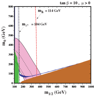
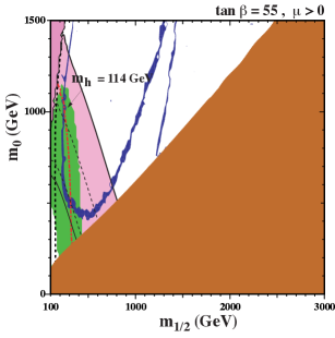
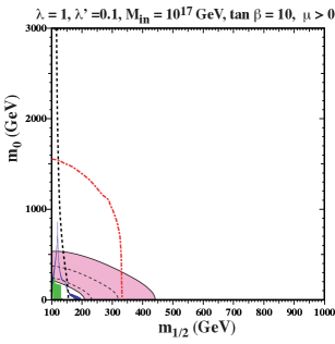
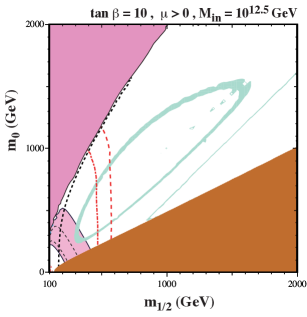
Figure 1: The $(m_{1/2},m_{0})$ planes for (upper left) the CMSSM with $\tan\beta=10$ and (upper right) $\tan\beta=55$ JEEOSS , (lower left) assuming SU(5) universality at $10^{17}$ GeV with representative choices of the quartic GUT Higgs couplings JEEMO , and (lower right) assuming scalar mass universality at $10^{12.5}$ GeV JEEOS2 , all assuming $\mu>0,A_{0}=0,m_{t}=173.1$ GeV and $m_{b}(m_{b})^{\overline{MS}}_{SM}=4.25$ GeV. The near-vertical (red) dot-dashed lines are the contours $m_{h}=114$ GeV JELEPH , and the near-vertical (black) dashed line is the contour $m_{\chi^{\pm}}=104$ GeV JELEPsusy . The medium (dark green) shaded region is excluded by $b\to s\gamma$, and the dark (blue) shaded area is the cosmologically preferred region JEWMAP . In the dark (brick red) shaded region, the LSP is the charged lighter stau slepton. The region allowed by the E821 measurement of $g_{\mu}-2$ at the 2-$\sigma$ level, is shaded (pink) and bounded by solid black lines, with dashed lines indicating the 1-$\sigma$ ranges.

0.13 Global Supersymmetric Fits

Within the general CMSSM and NUHM frameworks, is it possible to find a preferred region of supersymmetric masses? To answer this question, we adopted a frequentist approach and constructed a global likelihood function using precision electroweak data, the LEP Higgs mass limit (allowing for theoretical uncertainties), the cold dark matter density, $b\to s\gamma$ and $B_{s}\to\mu^{+}\mu^{-}$ constraints and (optionally) $g_{\mu}-2$ JEMC1 ; JEMC2 ; JEMC3 .

In both the CMSSM and the NUHM1 we found that small $m_{1/2}$ and $m_{0}$ in the coannihilation region are preferred, with the focus-point region disfavoured. The best-fit points, 68% and 95% CL regions in the $(m_{0},m_{1/2})$ planes of the CMSSM and NUHM1 are shown in Fig. 2 JEMC2 , and the corresponding spectra are shown in Fig. 3 JEMC3 . The favoured areas of the planes shown in Fig. 2 are quite sensitive to the treatments of the constraints, particularly $g_{\mu}-2$ and $b\to s\gamma$ JEMC2 . In the extreme case when the $g_{\mu}-2$ constraint is dropped entirely, as in Fig. 4, large values of $m_{0}$ are no longer strongly disfavoured, although the other constraints still show some slight preference for small $m_{0}$ JEMC3 .

Figure 2: The $(m_{0},m_{1/2})$ planes for (left) the CMSSM and (right) the NUHM1. The dark shaded area at low $m_{0}$ and high $m_{1/2}$ is excluded due to a scalar tau LSP, and the light shaded areas at low $m_{1/2}$ do not exhibit electroweak symmetry breaking. The nearly horizontal line at $m_{1/2}\approx 160$ GeV in the lower panel has $m_{\tilde{\chi}_{1}^{\pm}}=103$ GeV, and the area below is excluded by LEP searches. Just above this contour at low $m_{0}$ in the lower panel is the region that is excluded by trilepton searches at the Tevatron. Shown in each plot is the best-fit point, indicated by a filled circle, and the 68 (95)% C.L. contours from our fit as dark grey/blue (light grey/red) overlays JEMC2 . Also shown are 5-$\sigma$ discovery contours at the LHC with the indicated luminosities and centre-of-mass energies.

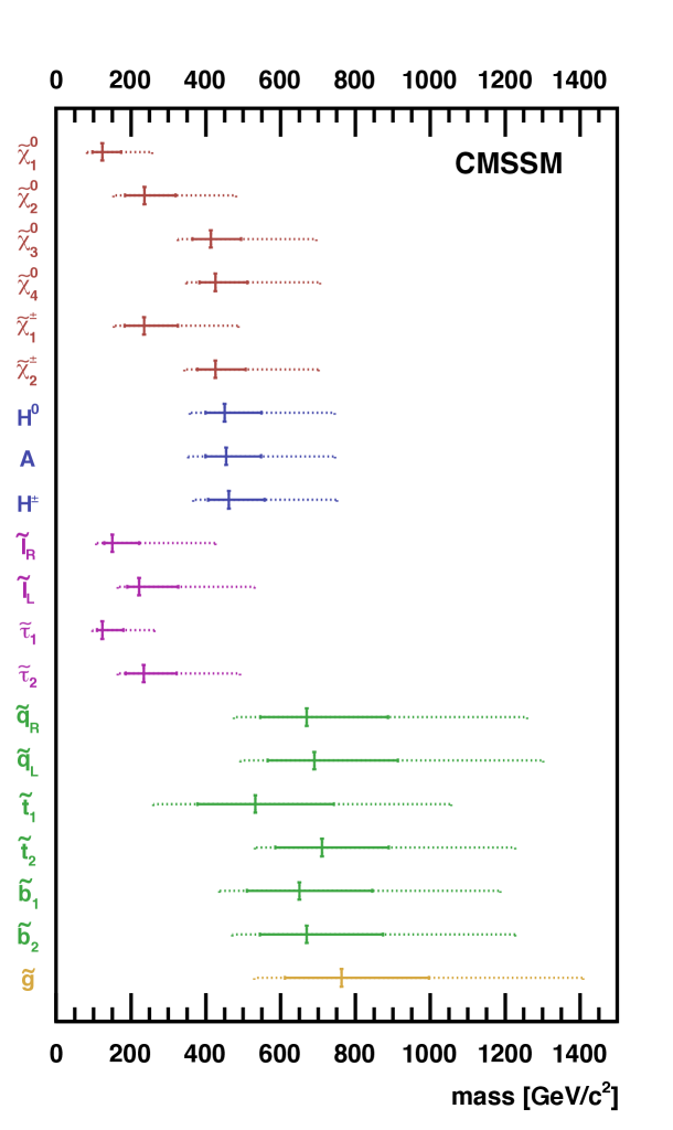
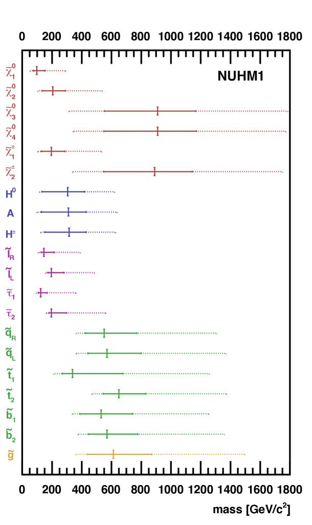
Figure 3: Spectra in the CMSSM (left) and the NUHM1 (right). The vertical solid lines indicate the best-fit values, the horizontal solid lines are the 68% C.L. ranges, and the horizontal dashed lines are the 95% C.L. ranges for the indicated mass parameters JEMC3 .

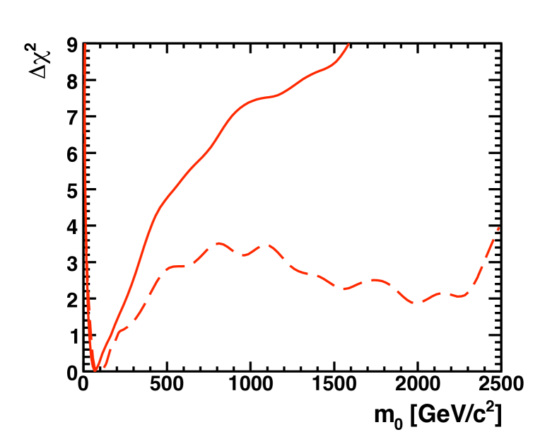
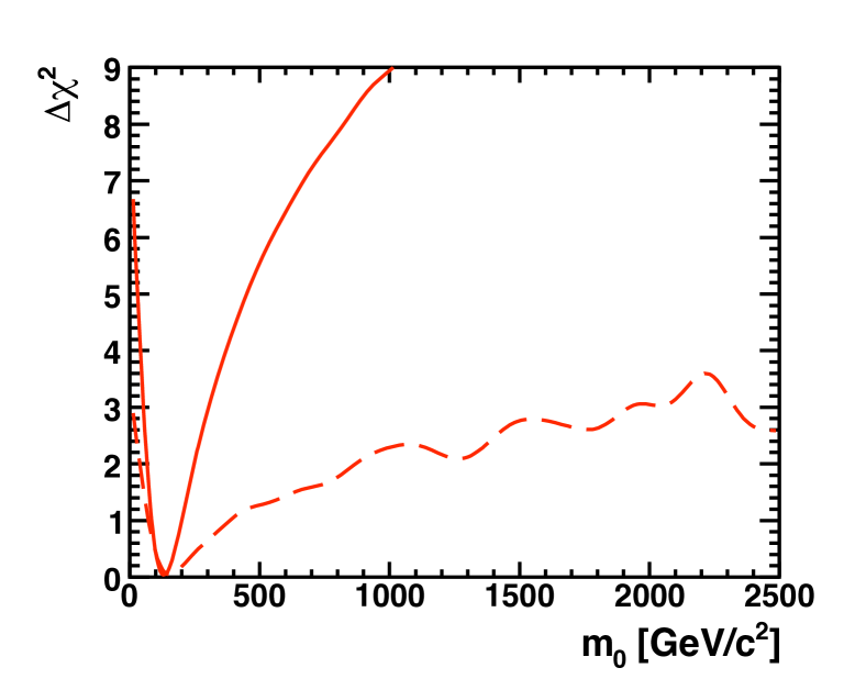
Figure 4: The likelihood functions for $m_{0}$ in the CMSSM (left plot) and in the NUHM1 (right plot). The $\chi^{2}$ values are shown including (excluding) the $g_{\mu}-2$ constraint as the solid (dashed) curves JEMC3 .

Fig. 2 also shows the expected sensitivity of the LHC for a discovery of supersymmetry with 5-$\sigma$ significance for varying LHC energies and luminosities. We see that there may be a fair chance to discover supersymmetry even in early LHC data. However, at the 95% CL, supersymmetry might still lie beyond the reach of the LHC with 1/fb of data at 14 TeV, as could also be inferred from the 95% CL ranges in Fig. 3.

0.14 Detecting Supersymmetric Dark Matter

Several strategies for the detection of WIMP dark matter particles such as the LSP have been proposed, including the direct search for scattering on nuclei in the laboratory JEGW , the search for energetic neutrinos produced by WIMP annihilations in the core of the Sun or Earth JEnus , the search for energetic photons produced by WIMP annihilations in the galactic centre or elsewhere in the Universe JEgammas , and the searches for positrons, antiprotons, etc., produced by WIMP annihilations in the galactic halo JEpbars .

As seen in Fig. 5, within the global fits to supersymmetric model parameters discussed earlier, our predictions for the direct nuclear scattering rates in the CMSSM and NUHM1 lie somewhat below the sensitivities of the CDMS and Xenon10 experiments, but within reach of planned upgrades of these experiments JEMC3 . Subsequently, the CDMS II JECDMSII and Xenon100 JEXe100 experiments have announced results with somewhat improved sensitivity. In particular, the CDMS II experiment reported two events with relatively low recoil energies (corresponding possibly to the scattering of a WIMP weighing $<30$ GeV) where less than one event was expected JECDMSII , but this hint was not confirmed by the Xenon100 experiment in its initial 11-day test run JEXe100 . (Nor have possible signals in the DAMA/LIBRA JEDAMA and CoGeNT experiments JECoGeNT been confirmed by either CDMS or Xenon100.) It is expected that updated Xenon100 results with much greater sensitivity will be announced soon, reaching significantly into the scattering rates expected within our global fits. (Though it should be noted that these predictions assume one particular value for the spin-independent scattering matrix element, which is a significant source of uncertainty in the predictions JEEOSavage1 .)

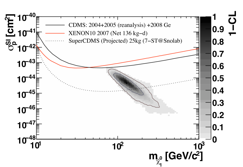
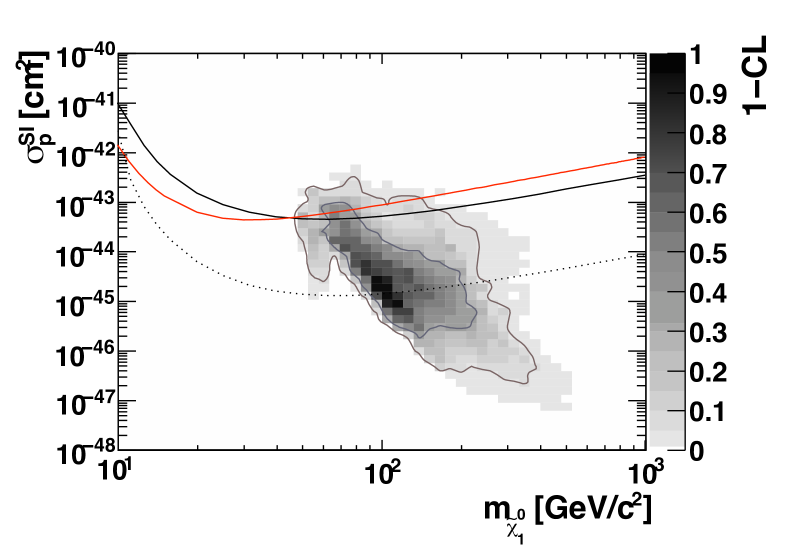
Figure 5: The correlation between the spin-independent dark matter scattering cross section and $m_{\chi}$ in the CMSSM (left panel) and in the NUHM1 (right panel). The solid lines JEDMtool are the experimental upper limits from CDMS JECDMS and Xenon10JEXe10 , The dashed line JEDMtool indicates the projected sensitivity of the SuperCDMS experiment JEsuperCDMS : that of Xenon100 may be similar.

The next most promising strategy for indirect detection of dark matter may be the search for energetic neutrinos emitted by WIMP annihilations in the core of the Sun JEnus . It is often assumed that the annihilation rate is in equilibrium with the WIMP capture rate, but this is not true in general in the CMSSM JEEOSavage . Nor is spin-dependent scattering the dominant mechanism for LSP capture by the Sun, as is often assumed: spin-independent scattering on heavier elements inside the Sun may also be important, even dominant JEEOSavage . As seen in Fig. 6, in a general survey of the CMSSM parameter space JEEOSavage , we find significant portions of the focus-point strips, and some parts of the coannihilation strips, where the flux of energetic neutrinos due to LSP annihilations may be detectable in the IceCube/DeepCore experiment JEICDC .

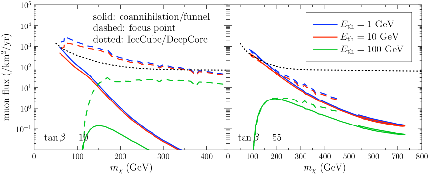
Figure 6: The CMSSM muon fluxes though a detector calculated for $A_{0}=0$ and (left) $\tan\beta=10$, (right) $\tan\beta=55$, along the WMAP strips in the coannihilation/funnel regions (solid) and the focus-point region (dashed) JEEOSavage . Fluxes are shown for muon energy thresholds of (top to bottom) 1 GeV, 10 GeV, and 100 GeV. Also shown is a conservative estimate of the sensitivity of the IceCube/DeepCore detector (dotted) JEICDC , normalized to a muon threshold of 1 GeV, for a particular hard annihilation spectrum that is a rough approximation to that expected in CMSSM models.

0.15 The Start-up of the LHC

The LHC made its first collisions on November 29th, 2009, and its first 7-TeV collisions on March 30th, 2010. Much jubilation, but where are the Higgs boson and supersymmetry, you may ask. It should be recalled that the total proton-proton cross section for producing a new particle weighing $\sim 1$ TeV is $\sim 1$/TeV², possibly suppressed even further by small couplings $\sim\alpha^{2}$, whereas the total cross section $\sim 1/m_{\pi}^{2}$, so that the ‘interesting’ new physics signal is likely to occur in $\sim 10^{12}$ of the collisions. This is like looking for a needle in $\sim 100,000$ haystacks!

So far the LHC experiments have seen only a few $\times 10^{12}$ collisions. The missing $E_{T}$ distribution agrees perfectly with simulations over more than 6 orders of magnitude JEMET , and there is no sign yet of an excess of events that might be due to the production and escape of dark matter particles, whether they be LSPs, LKPs, LTPs, or whatever. Moreover, the kinematics of the events with missing $E_{T}$ is exactly what one would expect from mismeasured QCD events and other Standard Model backgrounds: no signs yet of new physics beyond the Standard Model.

The results of our frequentist likelihood analysis were compared in Fig. 2 with the estimated sensitivity of the LHC at or close to its design energy. In 2010 it has been operating at $\sim 7$ TeV and accumulating $\sim 50$/pb of integrated luminosity, which is sufficient to extend the reach for supersymmetry beyond the Tevatron. The centre-of-mass energy may be increased in 2011 to 8 or 9 TeV, and the objective is to accumulate $\sim 1$/fb of integrated luminosity. Fig. 7 shows the estimated sensitivity of supersymmetry searches with the ATLAS experiment JEATLAS7 using 1/fb of data at 7 TeV. Comparing with Fig. 2, we see that the best-fit points in the CMSSM and NUHM1 should lie within reach. There are significant prospects for soon getting some interesting news about supersymmetry, one way or the other.

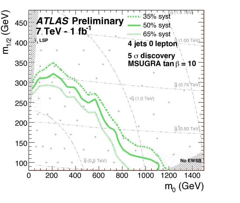
Figure 7: The sensitivity in the $(m_{0},m_{1/2})$ plane of the ATLAS experiment for a 5-$\sigma$ discovery of a supersymmetric signal with 1/fb at 7 TeV in the centre of mass.

0.16 A Conversation with Mrs. Thatcher

In 1982, Mrs. Thatcher, the British Prime Minister at the time, visited CERN, and I was introduced to her as a theoretical physicist. “What exactly do you do?”, she asked in her inimitably intimidating manner. “I think of things for experimentalists to look for, and then I hope they find something different”, I responded. Somewhat predictably, Mrs. Thatcher asked “Wouldn’t it be better if they found what you predicted?” My response was that ”If they found exactly what the theorists predicted, we would not be learning so much”. In much the same spirit, I hope (and indeed expect) that the LHC will become most famous for discovering something that I did NOT discuss in this talk - as long as it casts light on dark matter!

Extra Dimensional Metric Reversal Symmetry and its Prospect for Cosmological Constant and Zero-point Energy Problems, Automatic Pauli-Villars-like Regularization, and an Interesting Kaluza-Klein Spectrum R. ErdemE-mail:recaierdem@iyte.edu.tr

0.17 Introduction: Metric reversal symmetry and the cosmological constant problem

In this talk I will consider a symmetry that may be called metric reversal symmetry, in particular, the extra dimensional representations of this symmetry. This symmetry, first, was introduce in re1Erdem1 as a possible solution to cosmological constant (CC) problem re1Weinberg in a classical setting in extra dimensions. Below I define the metric reversal symmetry and mention its use for CC problem. In the following sections I review my recent studies on the use of this symmetry at quantum level, namely, zero-point energy problem, an interesting Kaluza-Klein spectrum, an automatic Pauli-Villars-like regularization, and some of their possible implications.

Metric reversal is defined by

$$ds^{2}\,=\,g_{AB}dx^{A}dx^{B}\,\rightarrow\,-ds^{2}$$ (210)

This transformation has two realizations: The first re1Erdem1 ; re1Nobbenhuis ; re1tHooft is

$$x^{A}\,\rightarrow\,i\,x^{A}~{},~{}~{}g_{AB}\,\rightarrow\,g_{AB}$$ (211)

The second re1Bonelli ; re1Erdem2 ; re1DuffKalk is

$$x^{A}\,\rightarrow\,x^{A}~{},~{}~{}g_{AB}\,\rightarrow\,-\,g_{AB}$$ (212)

Metric reversal symmetry (MRS) may be imposed at the level of the equations of motion (EM) (e.g. Einstein equations) by requiring the equations be covariant under MRS or at the level of the action by requiring the action be invariant under MRS. MRS forbids a CC in any dimension if it is imposed at the level of EM re1Nobbenhuis ; re1tHooft . MRS can be only classically viable if it is introduced at the level of EM. On the other hand MRS can be extended to the quantum domain if it is imposed to the action. So I prefer to impose MRS at the level of action functional. The gravitational action

$$S_{R}=\frac{1}{16\pi\,G}\int\sqrt{(-1)^{S}g}\,R\,d^{D}x$$ (213)

is invariant under either of (211) or (212) only in

$$D=2(2n+1)~{}~{}~{},~{}~{}~{}~{}n=0,1,2,3,....~{}~{}~{}.$$ (214)

while the CC action

$$S_{C}=\frac{1}{8\pi\,G}\int\sqrt{g}\,\Lambda\,d^{D}x.$$ (215)

is forbidden in $2(2n+1)$ dimensions.

So if our space is taken to be 2(2n+1) dimensional (or if the gravitation and the CC reside on a 2(2n+1) dimensional subspace of a larger space) then the cosmological constant (CC) is forbidden. In this framework the accelerated expansion of the universe may be attributed to a small breaking of MRS or to an alternative mechanism (such as quintessence, modified gravity etc.) if the symmetry is taken to be exact. Another point to to be mentioned is that two realizations of MRS are not equivalent in matter sector while they are wholly equivalent in the gravitational sector. For example $F_{AB}F^{AB}$ is odd under (211) while it is even under (212). So two realizations of MRS may be considered to be two different symmetries after the introduction of matter. As we shall see in the next section this point may be used to construct a model that solves zero-point energy problem as well. The details of these points and some other less major points may be found in re1Erdem1 ; re1Erdem2 ; re1Erdem3 .

0.18 Metric Reversal symmetry and zero-point energy problem

Quantization results in by-product energies that survive even in the absence of any particle. These energies (i.e. zero-point energies (ZPE)) are some kind of vacuum energy. They emerge as zero modes of harmonic oscillators or fields in quantum theory. The total ZPE associated with a particle is constant, and is found as the sum over the contributions due to different momenta, and is naively infinite. However ZPE is eliminated by subtracting ZPE from total energy. In the quantum field theory (QFT) in flat space this elimination (normal ordering) has no physical effect because changing the energy by a constant does not change the physical results. However in QFT in curved space this naive elimination of ZPE is not well-defined because gravity couples to all energies. So subtraction process affects the physical out-come. Moreover after normal ordering a non-zero vacuum energy remains and it is proportional to particle masses. So even the renormalized zero-point energy of electron gives a vacuum energy density that is $10^{36}$ times the observed energy density of the universe. This may be called ZPE problem. Renormalized ZPE may be identified by CC or as a different kind of vacuum energy depending on how the infinities are regulzarized in renormalization procedure. Moreover CC may get classical field theoretic contributions such as vacuum expectation of scalar feilds. Therefore it is better to consider ZPE problem separately.

In an attempt for a solution for ZPE one must take the following points into account: CC problem as well should be addressed. Therefore the dimension of the subspace we live in should be D = 2(2n+1). Another point is that It is easier to impose the symmetry so that ZPE vanishes instead of trying to make it small. This requires the symmetry be exact while the scale factor, $a(t)$ in Robertson-Walker metric breaks the symmetry generated by (211). Therefore both realizations of MRS should be used so that the realization of MRS generated by (212) is kept intact to impose ZPE vanish while the realization of MRS generated by (211)is broken. The following is the summary of a model that satisfies these criteria re1Erdem4 .

Consider a space consisting of the sum of 2(2n+1) and 2(2m+1) (e.g 6 and 2) dimensional subspaces with the metric

$$ds^{2} = g_{AB}dx^{A}\,dx^{B}\,+\,g_{A^{\prime}B^{\prime}}dx^{A^{\prime}}\,dx^{B^{\prime}}$$

$$= \Omega_{z}(z)[g_{\mu\nu}(x)\,dx^{\mu}dx^{\nu}\,+\,\tilde{g}_{ab}(y)\,dy^{a}dy^{b}]\,+\,\Omega_{y}(y)\tilde{g}_{A^{\prime}B^{\prime}}(z)\,dz^{A^{\prime}}dz^{B^{\prime}}$$

(217)

$$\Omega_{y}(y)\,=\,\cos{k|y|})~{}~{},~{}~{}~{}\Omega_{z}(z)\,=\,\cos{k^{\prime}|z|}$$

$$A,B = 0,1,2,3,5,....N~{}~{},~{}~{}~{}N=2(2n+1)$$

$$A^{\prime},B^{\prime} = 1^{\prime},2^{\prime},,....N^{\prime}~{}~{},~{}~{}~{}N^{\prime}=2(2m+1)$$

$$~{}~{}~{}~{}~{}~{}~{}~{}~{}~{}~{}\mu\nu=0,1,2,3~{},~{}~{}~{}a,b=1,2,...,N-4~{}~{},~{}~{}~{}n,m=0,1,2,3......~{}~{}.$$

The usual four dimensional space is embedded in the first space $g_{AB}dx^{A}\,dx^{B}$.

I assume that the gravitational sector is invariant under both realizations of MRS, that is, under

$$ds^{2}\,\rightarrow\,-\,ds^{2}~{}~{}~{}\mbox{as}~{}~{}~{}~{}x^{A}\,\rightarrow\,i\,x^{A}\,,~{}~{}x^{A^{\prime}}\,\rightarrow\,i\,x^{A^{\prime}}$$

$$g_{AB}\,\rightarrow\,g_{AB}\,,~{}~{}g_{A^{\prime}B^{\prime}}\,\rightarrow\,g_{A^{\prime}B^{\prime}}$$ (218)

$$\Rightarrow~{}~{}\Omega_{z}\,\rightarrow\,\Omega_{z}\,,~{}~{}\Omega_{y}\,\rightarrow\,\Omega_{y}$$

$$g_{\mu\nu}\,\rightarrow\,g_{\mu\nu}\,,~{}~{}\tilde{g}_{ab}\,\rightarrow\,\tilde{g}_{ab}\,,~{}~{}\tilde{g}_{A^{\prime}B^{\prime}}\,\rightarrow\,\tilde{g}_{A^{\prime}B^{\prime}}$$ (219)

and

$$ds^{2}\,\rightarrow\,-\,ds^{2}~{}~{}~{}\mbox{as}~{}~{}~{}~{}ky\,\rightarrow\,\pi\,-\,ky~{},~{}~{}k^{\prime}z\,\rightarrow\,\pi\,-\,k^{\prime}z$$

$$x^{A}\,\rightarrow\,x^{A}\,,~{}~{}x^{A^{\prime}}\,\rightarrow\,x^{A^{\prime}}$$ (220)

$$\Rightarrow~{}~{}\Omega_{z}\,\rightarrow\,-\Omega_{z}\,,~{}~{}\Omega_{y}\,\rightarrow\,-\Omega_{y}$$

$$g_{\mu\nu}\,\rightarrow\,g_{\mu\nu}\,,~{}~{}\tilde{g}_{ab}\,\rightarrow\,\tilde{g}_{ab}\,,~{}~{}\tilde{g}_{A^{\prime}B^{\prime}}\,\rightarrow\,\tilde{g}_{A^{\prime}B^{\prime}}~{}~{}.$$ (221)

Note that the requirements of the homogeneity and isotropy of the 4-dimensional space together with the equations (218-221) set $g_{\mu\nu}$ to the Minkowski metric $\eta_{\mu\nu}=diag(1,-1,-1,-1)$. Later (219) will be broken by a small amount in the matter sector to accommmodate the cosmic expansion.

The gravitational action is taken to be

$$S_{R} = \frac{1}{16\pi\,\tilde{G}}\int\,dV\,\tilde{R}^{2}$$ (222)

$$dV = dV_{1}\,dV_{2}~{},~{}~{}dV_{1}\,=\,\sqrt{g(-1)^{S}}\,d^{N}x~{},~{}~{}dV_{2}\,=\,\sqrt{g^{\prime}(-1)^{S^{\prime}}}\,d^{N^{\prime}}x^{\prime}$$

$$\tilde{R} = R(x,x^{\prime})+R^{\prime}(x,x^{\prime})$$ (224)

where the meaning of the primed and the unprimed quantities is evident from (218). After integration over extra dimensions $S_{R}$ becomes

$$S_{R} = \frac{M^{N+N^{\prime}-4}}{16\pi\,\tilde{G}}\int\sqrt{(-1)^{S}g}\sqrt{(-1)^{S^{\prime}}g^{\prime}}\,2\,R(x)\,R^{\prime}(x^{\prime})\,d^{N}x\,d^{N^{\prime}}x^{\prime}$$ (225)

$$= \frac{1}{16\pi\,G}\int\sqrt{(-1)^{S}g}\,R(x)\,\,d^{N}x$$

where

$$\frac{1}{16\pi\,G}\,=\,M_{pl}^{2}(\frac{M}{M_{pl}})^{2}M^{N+N^{\prime}-6}\frac{1}{16\pi\,\tilde{G}}\int\sqrt{(-1)^{S^{\prime}}g^{\prime}}\,2\,R^{\prime}(x^{\prime})\,d^{D}x^{\prime}$$ (226)

which is the usual Einstein-Hilbert action. The cosmological constant term is still forbidden by either realization of MRS.

Now we consider the subject that is the heart of this section, namely, the zero-point energies induced by the matter sector. Here we consider only the kinetic term of a scalar field here since this is enough to give the essential points of the formulation. The other details and consideration of the other fields can be found in re1Erdem4 . Consider the kinetic part of the Lagrangian, ${\cal L}_{Mk}$ for a scalar field (in the space given in (218)

$${\cal L}_{\phi\,k}\,=\,{\cal L}_{\phi\,k1}\,+\,{\cal L}_{\phi\,k2}$$ (227)

$${\cal L}_{\phi\,k1}\,=\,\frac{1}{2}g^{AB}\partial_{A}\phi\partial_{B}\phi~{}~{},~{}~{}~{}{\cal L}_{\phi\,k2}\,=\,\frac{1}{2}g^{A^{\prime}B^{\prime}}\partial_{A^{\prime}}\phi\partial_{B^{\prime}}\phi$$ (228)

For simplicity I take $g_{\mu\nu}=\eta_{\mu\nu}$. Then the corresponding action is

$$S_{Mk} = \int\,dV\,{\cal L}_{Mk}$$ (229)

$$= \frac{1}{2}\int\,\sqrt{(-1)^{S}g}\sqrt{(-1)^{S^{\prime}}g^{\prime}}\,d^{D}x\,d^{D}x^{\prime}[\frac{1}{2}g^{AB}\partial_{A}\phi\partial_{B}\phi\,+\,\frac{1}{2}g^{A^{\prime}B^{\prime}}\partial_{A^{\prime}}\phi\partial_{B^{\prime}}\phi]$$

$$= \frac{1}{2}\int\,d^{4}x\,dy_{1}dy_{2}dz_{1}dz_{2}\,\Omega_{z}^{3}\Omega_{y}\,\{\Omega_{z}^{-1}[\eta^{\mu\nu}\partial_{\mu}\phi\partial_{\nu}\phi\,-\,(\frac{\partial\phi}{\partial y_{1}})^{2}\,-\,(\frac{\partial\phi}{\partial y_{2}})^{2}]$$

$$\,-\,\Omega_{y}[(\frac{\partial\phi}{\partial z_{1}})^{2}\,+\,(\frac{\partial\phi}{\partial z_{2}})^{2}]\,\}$$

$$= \frac{1}{2}LL^{\prime}\int\,d^{4}x\,\int_{0}^{L}\int_{0}^{L^{\prime}}dydz\,\cos^{3}{k^{\prime}z}\cos{ky}\{\cos^{-1}{k^{\prime}z}[\eta^{\mu\nu}\partial_{\mu}\phi\partial_{\nu}\phi\,\,-\,(\frac{\partial\phi}{\partial y})^{2}]$$

$$\,-\,\cos^{-1}{ky}(\frac{\partial\phi}{\partial z})^{2}\}$$

where $y=y_{2}$, $z=z_{2}$ is adopted.

$\phi$ may be Fourier decomposed as

$$\phi\,=\,\phi_{AA}(x,y,z)\,+\,\phi_{AS}(x,y,z)\,+\,\phi_{SA}(x,y,z)\,+\,\phi_{SS}(x,y,z)$$

$$\phi_{AA}(x,y,z) = \sum_{n,m}\,\phi^{AA}_{n,m}(x)\,\sin{(n\,ky)}\,\sin{(m\,k^{\prime}z)}$$ (230)

$$\phi_{AS}(x,y,z) = \sum_{n,m}\,\phi^{AS}_{n,m}(x)\,\sin{(n\,ky)}\,\cos{(m\,k^{\prime}z)}$$ (231)

$$\phi_{SA}(x,y,z) = \sum_{n,m}\,\phi^{SA}_{n,m}(x)\,\cos{(n\,ky)}\,\sin{(m\,k^{\prime}z)}$$ (232)

$$\phi_{SS}(x,y,z) = \sum_{n,m}\,\phi^{SS}_{n,m}(x)\,\cos{(n\,ky)}\,\cos{(m\,k^{\prime}z)}$$

$$k=\frac{\pi}{L}~{},~{}k^{\prime}=\frac{\pi}{L^{\prime}}~{},~{}~{}0\leq\,y\,\leq\,L~{},~{}~{}0\leq\,z\,\leq\,L^{\prime}~{}~{},~{}~{}~{}n,m=0,1,2,.....$$

where we have used $k=\frac{\pi}{L}$, $k^{\prime}=\frac{\pi}{L^{\prime}}$ since $0\leq\,y\,\leq\,L$, $0\leq\,z\,\leq\,L^{\prime}$. After replacing this expansion in (229) and requiring the action be invariant under extra dimensional parity one obtains

$$S_{Mk} = \frac{1}{2}LL^{\prime}\int\,d^{4}x\,\{\eta^{\mu\nu}\sum_{n,m,r,s}\partial_{\mu}(\,\phi_{n,m}(x)\,)\,\partial_{\nu}(\,\phi_{r,s}(x)\,)$$

$$\qquad\qquad\times\,\int_{0}^{L}\,dy\,\cos{ky}\,\sin{(n\,k|y|)}\sin{(r\,k|y|)}$$

$$\qquad\qquad\qquad\int_{0}^{L^{\prime}}\,dz\,\cos^{2}{k^{\prime}z}\sin{(m\,k^{\prime}|z|)})\,\sin{(s\,k^{\prime}|z|)})$$

$$\,-k^{2}\,\,\sum_{n,m,r,s}\,nr\,\phi_{n,m}(x)\,\phi_{r,s}(x)\,\int_{0}^{L}\,dy\,\cos{ky}\,\,\cos{(n\,k|y|)}\cos{(r\,k|y|)}$$

$$\qquad\qquad\times\,\int_{0}^{L^{\prime}}\,dz\,\cos^{2}{k^{\prime}z}\sin{(m\,k^{\prime}|z|)})\,\sin{(s\,k^{\prime}|z|)})\}$$

$$\,-k^{\prime 2}\,\,\sum_{n,m,r,s}\,ms\,\phi_{n,m}(x)\,\phi_{r,s}(x)\,\int_{0}^{L}\,dy\,\sin{(n\,k|y|)}\sin{(r\,k|y|)}$$

$$\qquad\qquad\times\,\int_{0}^{L^{\prime}}\,dz\,\cos^{3}{k^{\prime}z}\cos{(m\,k^{\prime}|z|)})\,\cos{(s\,k^{\prime}|z|)})=$$

$$= \frac{1}{32}(LL^{\prime})^{2}\int\,d^{4}x\,\{\eta^{\mu\nu}\sum_{r,s}$$ (235)

$$\partial_{\mu}\bigl{[}\,\phi_{r-1,s-2}(x)\,+\,\phi_{r-1,s+2}(x)\,-\,\phi_{r-1,-s-2}(x)\,-\,\phi_{r-1,2-s}(x)$$

$$\,+\,2\phi_{r-1,s}(x)-\,2\,\phi_{r-1,-s}(x)\,+\,\phi_{r+1,s-2}(x)\,$$

$$+\,(\,\phi_{r+1,s+2}(x)\,-\,\phi_{r+1,-s-2}(x)\,-\,\phi_{r+1,2-s}(x)\,$$

$$+\,2\phi_{r+1,s}(x)-\,2\phi_{r+1,-s}(x)\,-\,\phi_{-r-1,s-2}(x)\,)$$

$$\,-\,\phi_{-r-1,s+2}(x)\,+\,\phi_{-r-1,-s-2}(x)\,+\,\phi_{-r-1,2-s}(x)-\,2\phi_{-r-1,s}(x)\,$$

$$+\,2\phi_{-r-1,-s}(x)\,-\,\phi_{1-r,s-2}(x)\,-\,\phi_{1-r,s+2}(x)\,+\,\phi_{1-r,-s-2}(x)$$

$$+\,\phi_{1-r,2-s}(x)\,-\,2\phi_{1-r,s}(x)\,+\,2\phi_{1-r,-s}(x)\,\bigr{]}\partial_{\nu}(\,\phi_{r,s}(x)\,)$$

$$\,-k^{2}\,\,\sum_{r,s}\,r\bigl{[}\,(r-1)(\,\phi_{r-1,s-2}(x)\,-\,\phi_{1-r,s-2}(x)\,)\,$$

$$+\,(r-1)(\phi_{r-1,s+2}(x)\,-\,\phi_{1-r,s+2}(x)\,)$$

$$-\,(r-1)(\,\phi_{r-1,-s-2}(x)\,-\,\phi_{1-r,-s-2}(x)\,)\,$$

$$-\,(r-1)(\,\phi_{r-1,2-s}(x)\,-\,\phi_{1-r,2-s}(x)\,)+\,2(r-1)(\,\phi_{r-1,s}(x)\,-\,\phi_{1-r,s}(x)\,)\,$$

$$-\,2(r-1)(\,\phi_{r-1,-s}(x)\,-\,\phi_{1-r,-s}(x)\,)$$

$$+\,(r+1)(\,\phi_{r+1,s-2}(x)\,-\,\phi_{-r-1,s-2}(x)\,)$$

$$\,+\,(r+1)(\,\phi_{r+1,s+2}(x)\,-\,\phi_{-r-1,s+2}(x)\,)$$

$$-\,(r+1)(\,\phi_{r+1,-s-2}(x)\,-\,\phi_{-r-1,-s-2}(x)\,)$$

$$\,-\,(r+1)(\,\phi_{r+1,2-s}(x)\,-\,\phi_{-r-1,2-s}(x)\,)+\,2(r+1)(\,\phi_{r+1,s}(x)\,-\,\phi_{-r-1,s}(x)\,)$$

$$\,-\,2(r+1)(\,\phi_{r+1,-s}(x)\,-\,\phi_{-r-1,-s}(x)\,)\,\bigr{]}\phi_{r,s}(x)$$

$$\,-\frac{1}{2}k^{\prime 2}\,\,\sum_{r,s}\,s\,\bigl{[}\,(s-3)(\,\phi_{r,s-3}(x)\,-\,\phi_{r,3-s}(x)\,)$$

$$\,+\,(s+3)(\,\phi_{r,s+3}(x)\,-\,\phi_{r,-s-3}(x)\,)+\,3(s-1)(\,\phi_{r,s-1}(x)\,-\,\phi_{r,1-s}(x)\,)$$

$$\,+\,3(s+1)(\,\phi_{r,s+1}(x)\,-\,\phi_{r,-s-1}(x)\,)+\,(3-s)(\,\phi_{-r,s-3}(x)\,-\,\phi_{-r,3-s}(x)\,)$$

$$\,+\,(s+3)(\,\phi_{-r,-s-3}(x)\,-\,\phi_{-r,s+3}(x)\,)$$

$$+\,3(1-s)(\,\phi_{-r,s-1}(x)\,-\,\phi_{-r,1-s}(x)\,)$$

$$\,-\,3(s+1)(\,\phi_{-r,s+1}(x)\,-\,\phi_{-r,-s-}(x)\,)\,\bigr{]}\,\phi_{r,s}(x)\}.$$

We notice that the odd modes are coupled to even modes and vica versa. In fact this is a result of the invariance under $ky^{a}\rightarrow\,\pi-ky^{a}$, $k^{\prime}\,z^{a}\rightarrow\,\pi-k^{\prime}\,z^{a}$ that enforces the coupling of even and odd modes to compensate the minus coming from the volume element in the action.

This makes the energy-momentum tensor $T_{\mu\nu}$ be of the same form in the extra dimensional Fourier modes. The replacement of the expansion of the modes in terms of creation and annihilation operators

$$\phi_{n,m}(x)\,=\,\sum_{\mathchoice{\mbox{\boldmath$\displaystyle k$}}{\mbox{\boldmath$\textstyle k$}}{\mbox{\boldmath$\scriptstyle k$}}{\mbox{\boldmath$\scriptscriptstyle k$}}}\,[\,a_{n,m}(\mathchoice{\mbox{\boldmath$\displaystyle k$}}{\mbox{\boldmath$\textstyle k$}}{\mbox{\boldmath$\scriptstyle k$}}{\mbox{\boldmath$\scriptscriptstyle k$}})\,\zeta(t)e^{i\mathchoice{\mbox{\boldmath$\displaystyle k$}}{\mbox{\boldmath$\textstyle k$}}{\mbox{\boldmath$\scriptstyle k$}}{\mbox{\boldmath$\scriptscriptstyle k$}}.\mathchoice{\mbox{\boldmath$\displaystyle x$}}{\mbox{\boldmath$\textstyle x$}}{\mbox{\boldmath$\scriptstyle x$}}{\mbox{\boldmath$\scriptscriptstyle x$}}}\,+\,a_{n,m}^{\dagger}(\mathchoice{\mbox{\boldmath$\displaystyle k$}}{\mbox{\boldmath$\textstyle k$}}{\mbox{\boldmath$\scriptstyle k$}}{\mbox{\boldmath$\scriptscriptstyle k$}})\,\zeta^{*}(t)e^{-i\mathchoice{\mbox{\boldmath$\displaystyle k$}}{\mbox{\boldmath$\textstyle k$}}{\mbox{\boldmath$\scriptstyle k$}}{\mbox{\boldmath$\scriptscriptstyle k$}}.\mathchoice{\mbox{\boldmath$\displaystyle x$}}{\mbox{\boldmath$\textstyle x$}}{\mbox{\boldmath$\scriptstyle x$}}{\mbox{\boldmath$\scriptscriptstyle x$}}}\,]$$ (236)

in the energy momentum tensor

$$T_{\mu}^{\nu}=\sum_{m,n,r,s}\partial_{\mu}\phi_{n,m}(x)\,\partial^{\nu}\phi_{r,s}(x)\,-\,g_{\mu}^{\nu}{\cal L}$$ (237)

results in the terms of the form

$$<0|T^{\nu}_{\mu}|0> \propto <0|\,a_{n,m}a_{r,s}^{\dagger}|0>\,=\,0~{},~{}~{}<0|\,a_{r,s}^{\dagger}a_{r,s}|0>\,=\,0$$

$$~{}~{}~{}~{}n\neq r~{}~{}~{}~{}\mbox{and/or}~{}~{}~{}~{}m\neq s$$

(because $a_{r,s}|0>\,=\,0$, and $[\,a_{n,m},a_{r,s}^{\dagger}\,]\,=\,0$ for $n\neq r$ and/or $m\neq s$) . In other words there is no contribution to vacuum energy density due to zero-point energies in this scheme. This solves the zero point-energy problem.

0.19 Metric reversal symmetry and an interesting Kaluza-Klein spectrum

In this section we shall consider a model where all except a finite number of Kaluza-Klein modes (i.e. the extra dimenional Fourier modes) are screened by the conformal factor in the metric. Note that both the form of the conformal factor and the form of the mixing of the Kaluza-Klein modes are determined by MRS. The details of the analysis given here may be found in re1Erdem5 . In this scheme it is not enough to produce a mode to in order to detect it have high enough energies to produce the mode but it is also necessary to have them high enough momenta relative to the detector (to expose to the sizes smaller than the extra dimension(s)). Therefore it has interesting phenomenological implications.

Adopt the following 5-dimensional space

$$ds^{2}\;=\;\cos{k\,z}\,[\,\eta_{\mu\nu}(x)\,dx^{\mu}dx^{\nu}-\,dz^{2}\,]~{}~{}~{}~{}~{}~{}~{}~{}\mu,\nu\,=\,0,1,2,3$$ (239)

where the extra dimension is taken to be compact and have the size $L$, and $k\,=\,\frac{2\pi}{L}$. Consider fermions with the action

$$S_{f} = \int(\cos{kz})^{\frac{5}{2}}\,{\cal L}_{f}\,d^{4}x\,dz$$

$$= \int(\cos{kz})^{2}\,\,i\bar{\chi}\gamma^{a}(\,\partial_{a}\,+\,\frac{1}{16}\tan{kz}\,[\,\gamma_{a}\;,\;\gamma_{5}]\,)\chi\;d^{4}x\,dz\;+\,H.C.$$

$$\{\gamma^{a},\gamma^{b}\}\,=\,2\eta^{ab}~{}~{},~{}~{}(\eta^{ab})=diag(1,-1,-1,-1,-1)$$

where $H.C.$ stands for Hermitian conjugate, and the term with the coefficient $\frac{1}{16}$ is the spin connection term.

We impose the following symmetries on the action

$$k\,z\, \rightarrow \,\pi\,+\,k\,z.$$ (241)

$$x^{a}\, \rightarrow \,-x^{a}~{}~{}~{}a=0,1,2,3,4$$ (242)

$$\chi_{n}(x)~{} \rightarrow ~{}\epsilon^{\lambda_{n}}\,{\cal CPT}\,\chi_{n}(-x)~{}~{}~{}~{}~{},~{}~{}~{}~{}~{}\lambda_{n}=\frac{i}{2}(-1)^{\frac{n}{2}}$$ (243)

where the superscript $a$ refers to the tangent space, $\epsilon$ is some constant, and ${\cal CPT}$ denotes the usual 4-dimensional CPT operator (acting on the spinor part of the field). We also impose anti-periodic boundary conditions in the extra dimension i.e. $\chi(x,z)=-\chi(x,z+2\pi\,L)$.

The extra dimensional Fourier expansion of $\chi$ in the light of invariance under

$$\chi = \chi_{\cal A}\,+\,\chi_{\cal S}$$ (244)

$$\chi_{\cal A}\left(x,z\right) = \sum_{|n|=1}^{\infty}\,\tilde{\chi}^{\cal A}_{|n|}\left(x\right)\,\,\sin{\left(\frac{1}{2}|n|\,kz\right)}$$ (245)

$$\chi_{\cal S}\left(x,z\right) = \chi_{0}\left(x\right)\,+\,\sum_{|n|=1}^{\infty}\,\tilde{\chi}^{\cal S}_{|n|}(x)\,\,\cos{\left(\frac{1}{2}|n|\,kz\right)}$$ (246)

$$\tilde{\chi}^{{\cal A}({\cal S})}_{|n|}\left(x\right) = \,\chi^{{\cal A}({\cal S})}_{n}\left(x\right)\,-(+)\,\chi^{{\cal A}({\cal S})}_{-n}(x)$$

where $n$ are odd integers (due to anti-boundary conditions in the $z$-direction), the absolute value signs in $|n|$ is used to emphasize the positiveness of $n$ (due to the symmetry $x^{a}\rightarrow\,-x^{a}$).

After replacing (244) in (0.19) we obtain

$$\sum_{r,s=0}^{\infty}\int\,d^{4}x\,i\bar{\chi}_{\left(2|r|+1\right)}\gamma^{\bar{\mu}}\partial_{\bar{\mu}}\chi_{\left(2|s|+1\right)}\times\,2\,\int\,dz\,\left(\cos{kz}\right)^{2}\,$$

$$\qquad\left[\cos{\frac{2|r|+1}{2}kz}\,\cos{\frac{2|s|+1}{2}kz}\,-\,\sin{\frac{2|r|+1}{2}kz}\,\sin{\frac{2|s|+1}{2}kz}\,\right]\,+\,H.C.$$

$$= \sum_{r,s=0}^{\infty}\int\,d^{4}x\;i\bar{\chi}_{\left(2|r|+1\right)}\gamma^{\bar{\mu}}\partial_{\bar{\mu}}\chi_{\left(2|s|+1\right)}\,$$

$$\qquad\qquad\int_{0}^{L}\,dz\,\left(\cos{2kz}+1\right)\,\cos{\left(|r|+|s|+1\right)kz}\,\,+\,H.C.$$

$$= \frac{1}{2}\sum_{r,s=0}^{\infty}\,\int\,d^{4}x\,i\bar{\chi}_{\left(2|r|+1\right)}\gamma^{\bar{\mu}}\partial_{\bar{\mu}}\chi_{\left(2|s|+1\right)}\,\int_{0}^{L}\,dz\,\left[\,\cos{\left(|r|+|s|-1\right)kz}\,\right]\,+\,H.C.$$

where $2r+1=4l+1$, $2s+1=4p+3$ (l,p=0,1,2,….) or vica versa. The non-zero contribution to (LABEL:re1a8) are due to the terms where the arguments of the cosine functions are zero (or multiples of $2\pi$) i.e. the modes that satisfy

$$|r|+|s|-1=0~{}~{}~{}\Rightarrow~{}~{}~{}~{}~{}r=0~{}~{},~{}~{}s=1~{}~{}~{}~{}\mbox{or}~{}~{}~{}~{}s=1~{}~{},~{}~{}r=0$$ (248)

Therefore the result of the integration in (LABEL:re1a8) is

$$\frac{L}{2}\int\,d^{4}x\left[\,i\bar{\chi}_{1}\gamma^{\bar{\mu}}\partial_{\bar{\mu}}\chi_{3}\,+\,i\bar{\chi}_{3}\gamma^{\bar{\mu}}\partial_{\bar{\mu}}\chi_{1}\,\right]\,+\,H.C.$$ (249)

$$=\frac{1}{2}L\int\,d^{4}x\left[\,i\bar{\psi}\gamma^{\bar{\mu}}\partial_{\bar{\mu}}\psi\,-\,i\bar{\tilde{\psi}}\gamma^{\bar{\mu}}\partial_{\bar{\mu}}\tilde{\psi}\,\right]\,+\,H.C.$$ (250)

$$\psi\,=\,\frac{1}{\sqrt{2}}\left(\,\chi_{1}\,+\,\chi_{3}\,\right)~{}~{},~{}~{}\tilde{\psi}\,=\,\frac{1}{\sqrt{2}}\left(\,\chi_{1}\,-\,\chi_{3}\,\right)$$ (251)

This means that at scales larger than the size of the extra dimension (which effectively corresponds to integration over the extra dimension) only one fermion and one ghost fermion is observed. The other modes are only observed at smaller scales while they are screened at large extra dimensional length scales due to the screening because of the (the cosine) form of the conformal factor. These modes can be observed only in interactions with energies higher than the inverse size of the extra dimension. At distances greater than the size of the extra dimension(s) even when they are already excited they seem hidden (unless they have high relative momenta when they interact in the detector). In other words these modes behave like a strange form of dark matter. The experimental predictions of this model are quite different from the usual Kaluza-Klein prescription and need further study. In high energy colliders the signature of these modes would be a sudden increase in the strength of the interactions and a high correlation between the interacting particles. In my opinion the phenomenological implications of this scheme deserves a separate and detailed study by its own.

0.20 Metric reversal symmetry and an automatic Pauli-Villars-like regularization

In the usual Kaluza-Klein scheme, Kaluza-Klein tower is an additional source of infinites that should be regulated. This property of compact extra dimensions is one of the major problems of quantum field theory in extra dimensions. On the other we will see that in the spaces with metric reversal symmetry (MRS) there is the possibility of an automatic, Pauli-Villars-like on contary to the generic extra dimensional spaces. Below I summarize a model of this type. The details of this model may be found in re1Erdem6 .

Consider the following 7-dimensional space ($\mu,\nu\,=\,0,1,2,3$)

$$ds^{2}\;=\;g_{\mu\nu}(x)\,dx^{\mu}dx^{\nu}\,-\,\cos^{2}{k_{2}y_{2}}\,[\,\,dy_{1}^{2}\,+\,\cos^{2}{k_{3}y_{3}}dy_{2}^{2}\,+\,dy_{3}^{2}\,]$$ (252)

where the extra dimensions are compact and have the sizes $L_{1}$, $L_{2}$, $L_{3}$, and $k_{1}\,=\,\frac{2\pi}{L_{1}}$, $k_{2}\,=\,\frac{2\pi}{L_{2}}$, $k_{3}\,=\,\frac{2\pi}{L_{3}}$. Assume the symmetry

$$x^{a}\;\rightarrow\;-\,x^{a}~{}~{},~{}~{}~{}~{}a=0,1,2,3,5$$ (253)

$$x^{b}\;\rightarrow\;-\,x^{b}~{}~{},~{}~{}~{}~{}b=0,1,2,3,6$$ (254)

where $x^{5}=y_{1}$, $x^{6}=y_{2}$, $x^{7}=y_{3}$; and anti-periodic boundary conditions are adopted for the 5th and 6th directions while periodic boundary condition is adopted for the 7th direction for the field $\chi$ i.e. $\chi(x,z)=-\chi(x,z+L)$ for $z=y_{1}$, $L=L_{1}$ or $z=y_{2}$, $L=L_{2}$ while $\chi(x,y_{3})=\chi(x,y_{3}+L_{3})$. Then the Fourier expansion of a field $\chi$ is

$$\chi(x,z) = \sum_{n=1}^{\infty}\{\,f_{|n|}[\cos{(\frac{|n|kz}{2})}+\sin{(\frac{|n|kz)}{2})}]$$ (255)

$$+g_{|n|}[\cos{(\frac{|n|kz)}{2})}-\sin{(\frac{|n|kz)}{2})}]\}\chi_{|n|}(x)$$

where $z=y_{1},y_{2}$, $k=k_{1},k_{2}$, $a_{|n|}$, $b_{|n|}$, $f_{|n|}$, $g_{|n|}$ are some constants. Even and odd $n$ correspond to periodic and anti-periodic boundary conditions re1conformal , respectively. The modes $\chi_{n}$ are taken to transform under (253) and (254) as

$$\varphi_{n,m,r}(x)\,\rightarrow\,\xi^{\lambda_{n}}{\cal CPT}\,\varphi_{n,m,r}(-x)~{}~{}~{}~{}\mbox{as}~{}~{}~{}~{}x^{a}\,\rightarrow\,-x^{a}$$ (256)

$$\varphi_{n,m,r}(x)\,\rightarrow\,\xi^{\lambda_{m}}{\cal CPT}\,\varphi_{n,m,r}(-x)~{}~{}~{}~{}\mbox{as}~{}~{}~{}~{}x^{b}\,\rightarrow\,-x^{b}$$ (257)

$$\varphi_{n,m,r}(x)\,\rightarrow\,\xi^{\lambda_{n}+\lambda_{m}}{\cal CPT}\,\varphi_{n,m,r}(-x)$$

$$~{}\mbox{as}~{}~{}x^{a}\,\rightarrow\,-x^{a}~{},~{}x^{b}\,\rightarrow\,-x^{b}$$ (258)

$$\lambda_{n}=\frac{i}{2}(-1)^{\frac{n}{2}}~{}~{}~{}\lambda_{m}=\frac{i}{2}(-1)^{\frac{m}{2}}~{}~{}~{}~{}~{}a=0,1,2,3,5~{}~{};~{}~{}b=0,1,2,3,6$$

( where $n$, $m$, $r$ are the modes corresponding to $y_{1}$, $y_{2}$, $y_{3}$ directions, respectively; $\xi$ is some constant other than 1 or -1, and ${\cal CPT}$ denotes the part of (4-dimensional) CPT transformation acting on the spinor part of the field. I also impose the symmetry

$$k_{1}y_{1}\;\rightarrow\;k_{1}y_{1}\,+\,\pi$$ (259)

$$k_{2}y_{2}\;\rightarrow\;k_{2}y_{2}\,+\,\pi$$ (260)

In the light of the above observations I consider the following action

$$S_{fk1} = \int\,\;d^{4}x\,\,d^{3}y\,\cos^{3}{k_{2}y_{2}}\,\cos{k_{3}y_{3}}\frac{1}{2}[{\cal L}_{fk11}\,+\,{\cal L}_{fk12}]\;+\,H.C.$$ (261)

$${\cal L}_{fk11}\, = \,\frac{i}{4}[(\bar{\chi}_{(1)}\gamma^{\mu}\,\partial_{\mu}\chi_{(3)}+\bar{\chi_{(1)}}^{P}\gamma^{\mu}\,\partial_{\mu}\chi_{(3)}^{P})\,+\,y_{1}\rightarrow-y_{1}]$$ (262)

$${\cal L}_{fk12}\, = \,\frac{i}{4}[(\bar{\chi}\gamma^{\mu}\,\partial_{\mu}\chi^{P}-\bar{\chi}^{P}\gamma^{\mu}\,\partial_{\mu}\chi)+(y_{1}\rightarrow-y_{1})].$$ (263)

After inserting the explicit form of $\chi$ and imposing the symmetries (253), (254), (258), (260) one finds

$${\cal L}_{fk1} = \frac{1}{2}[{\cal L}_{fk11}\,+\,{\cal L}_{fk12}]$$

$$= \sum_{n_{1},m_{1}=1}^{\infty}\,A_{n1,m1}^{(1,3)}\,i\bar{\chi}_{n_{1}}(x,y)\gamma^{\mu}\partial_{\mu}\chi_{m_{1}}(x,y)\,\cos{\frac{n_{1}+m_{1}}{2}k_{1}y_{1}}\,+\,H.C.$$

where $y=y_{2},y_{3}$. The spectrum at the scales larger than the size of the extra dimensions may be found by integration of $[{\cal L}_{fk11}\,+\,{\cal L}_{fk12}]$ over the extra dimensions.

$$S_{fk1} = \int\,\;d^{4}x\,\,d^{2}y\,\cos^{3}{k_{2}y_{2}}\,\cos{k_{3}y_{3}}\sum_{n_{1},m_{1}=1}^{\infty}\,A_{n1,m1}^{(1,3)}\,i\bar{\chi}_{n_{1}}(x,y)\gamma^{\mu}\partial_{\mu}\chi_{m_{1}}(x,y)$$

$$\times\,\int\,dy_{1}\,\cos{\frac{n_{1}+m_{1}}{2}k_{1}y_{1}}\,+\,H.C.\;=\,0$$

$$A_{n1,m1}^{(1,3)}\,=\,(f_{n1}^{*}g_{m1}+g_{n1}^{*}f_{m1}+f_{n1}^{*}f_{m1}-g_{n1}^{*}g_{m1})$$

The upper index $*$ denotes complex conjugate, $H.C.$ stands for Hermitian conjugate, and $f_{n}$, $g_{n}$’s are those given in (255). The subscripts $(1)$, $(3)$, and the superscripts $(1,3)$ above refer to the modes with $n=4p+1$ and $n=4p+3$, respectively, where $p=0,1,2,.....$. The $y_{1}\rightarrow-y_{1}$ terms in the above equations stands for the term obtained from the previous one by replacing $y_{1}$’s in that term by $-y_{1}$ and insures the invariance of the Lagrangian ${\cal L}_{fk1}$ under (253). The values of $n_{1}$, $m_{1}$ in (263,0.20) are fixed by the requirement of invariance under (259), (256), and are given by

$$n_{1}\,=\,4l_{1}\,+\,1~{},~{}~{}m_{1}\,=\,4p_{1}\,+\,3~{}~{}~{}~{}\mbox{or vica versa}~{}~{}~{}~{}~{}~{}~{}~{}l_{1},p_{1}=0,1,2,.......$$ (266)

It is evident that (0.20) gives zero because $\int_{0}^{L_{1}}\,\cos{\frac{n_{1}+m_{1}}{2}k_{1}y_{1}}\,dy_{1}=0$ since $n_{1}+m_{1}\neq\,0$. Hence there are no observable fermions at scales larger than the sizes of the extra dimensions. Therefore an additional action must be introduced to accaount for the usual fermions while $S_{fk1}$ may be used for a Pauli-Villars-like regularization as we shall see. Assume that on the hyper-surface, $y_{3}=y_{1}$ the symmetry (253) (and (256) ) is broken by a small amount while there is an unbroken symmetry under the separate (and simultaneous) applications of (245), (246), and under the simultaneous application of (253) and (254) (and (256) and (257 ). Consider the following action that obeys these conditions

$$S_{fk2}\,=\epsilon\,\int\,\delta(k_{3}y_{3}-k_{1}y_{1})\cos^{3}{k_{2}y_{2}}\,\cos{k_{3}y_{3}}\frac{1}{2}[{\cal L}_{fk21}\,+\,{\cal L}_{fk22}]\;+\,H.C.$$ (267)

$${\cal L}_{fk21}\,=\,\frac{i}{8}[(\bar{\chi}_{(1,3)}\gamma^{\mu}\,\partial_{\mu}\chi_{(1,3)}+\bar{\chi}_{(1,3)}^{P1,P2}\gamma^{\mu}\,\partial_{\mu}\chi_{(1,3)}^{P1,P2}-\bar{\chi}_{(1,3)}^{P1}\gamma^{\mu}\,\partial_{\mu}\chi_{(1,3)}^{P1}-$$

$$\bar{\chi}_{(1,3)}^{P2}\gamma^{\mu}\,\partial_{\mu}\chi_{(1,3)}^{P2})+\,(y_{1,2}\rightarrow-y_{1,2})]$$ (268)

$${\cal L}_{fk22}\,=\,$$

$$\frac{i}{8}[(\bar{\chi}_{(1,3)}\gamma^{\mu}\,\partial_{\mu}\chi_{(1,3)}^{P1}+\bar{\chi}_{(1,3)}^{P1}\gamma^{\mu}\,\partial_{\mu}\chi_{(1,3)}-\bar{\chi}_{(1,3)}^{P2}\gamma^{\mu}\,\partial_{\mu}\chi_{(1,3)}^{P1,P2}-\bar{\chi}_{(1,3)}^{P1,P2}\gamma^{\mu}\,\partial_{\mu}\chi_{(1,3)}^{P2}$$

$$+\bar{\chi}_{(1,3)}\gamma^{\mu}\,\partial_{\mu}\chi_{(1,3)}^{P2}+\bar{\chi}_{(1,3)}^{P2}\gamma^{\mu}\,\partial_{\mu}\chi_{(1,3)}-\bar{\chi}_{(1,3)}^{P1}\gamma^{\mu}\,\partial_{\mu}\chi_{(1,3)}^{P1,P2}-\bar{\chi}_{(1,3)}^{P1,P2}\gamma^{\mu}\,\partial_{\mu}\chi_{(1,3)}^{P1}$$

$$+\bar{\chi}_{(1,3)}^{P1}\gamma^{\mu}\,\partial_{\mu}\chi_{(1,3)}^{P2}+\bar{\chi}_{(1,3)}^{P2}\gamma^{\mu}\,\partial_{\mu}\chi_{(1,3)}^{P1}+\bar{\chi}_{(1,3)}\gamma^{\mu}\,\partial_{\mu}\chi_{(1,3)}^{P1,P2}+\bar{\chi}_{(1,3)}^{P1,P2}\gamma^{\mu}\,\partial_{\mu}\chi_{(1,3)})$$

$$+(y_{1}\rightarrow-y_{1})]$$ (269)

where $\epsilon\,<<\,1$ is some constant that accounts for the breaking of the symmetry (253) by a small amount. The superscripts $P1$, $P2$ refer to the $\chi$’s transformed under (245), (246), respectively. After replacing the Fourier expansion of $\chi$ and integrating over extra dimensions one obtains

$$S_{fk2}\, = \,\frac{\epsilon L_{1}L_{2}L_{3}}{4\pi}(f_{1}^{*}g_{1}+g_{1}^{*}f_{1}+f_{1}^{*}f_{1}-g_{1}^{*}g_{1})$$ (270)

$$(f_{3}^{*}g_{3}+g_{3}^{*}f_{3}+f_{3}^{*}f_{3}-g_{3}^{*}g_{3})\int\,d^{4}x\,i\bar{\chi}_{13}\gamma^{\mu}\partial_{\mu}\chi_{13}$$

In other words only the mode $\chi_{13}$ is observed at large scales. If we take $n_{3}=0$ to be the lowest lying mode in $y_{3}$ direction then the usual fermions (i.e. the zero mode) are identified by $\chi_{130}$.

Although only $S_{fk2}$ is relavant on the brane $y_{1}=y_{3}$ and at large scales both of $S_{fk1}$ and $S_{fk2}$ are relavant on the brane. One must consider small patches in extra dimensional space to regulariza the affect of the delta function. Therefore we integrate ${\cal L}_{fk1}$ and $[{\cal L}_{fk21}+{\cal L}_{fk22}]$ on the patch

$$-\Delta\leq\,u\,\leq\Delta~{},~{}~{}~{}v\leq\,v^{\prime}\,\leq\,v+\Delta^{\prime}~{}~{}~{},~{}~{}~{}~{}u=k_{1}y_{1}-k_{3}y_{3}~{},~{}~{}v=k_{1}y_{1}+k_{3}y_{3}$$ (271)

The result of the integration may be expressed as

$$\int\,d^{4}x\,{\cal L}_{eff}$$ (272)

where

$${\cal L}^{eff}_{fk2} = \frac{i}{2}\lim_{x^{\prime}\rightarrow x}\partial_{\mu}\;\left(\,\bar{\chi}_{130}(x^{\prime}),\bar{\chi}_{310}(x^{\prime})\bar{\chi}_{330}(x^{\prime})\,\right)\,{\bf\tilde{M}}\,\gamma^{\mu}\left(\begin{array}[]{c}\chi_{130}(x)\\ \chi_{310}(x)\\ \chi_{330}(x)\end{array}\right)$$ (276)

here

$${\bf\tilde{M}} = \left(\begin{array}[]{ccc}\tilde{{\cal A}}&\tilde{{\cal B}}&\tilde{{\cal C}}\\ \tilde{{\cal B}}&\tilde{{\cal D}}&0\\ \tilde{{\cal C}}&0&0\end{array}\right)$$ (280)

where

$$\tilde{{\cal A}} \simeq \,\epsilon\cos^{3}{k_{2}y_{2}}\sum_{p_{1},s_{1}=0}^{\infty}\tilde{A}_{p_{1}s_{1}}^{(1,1)}\,\tilde{T}_{p_{1},s_{1}}^{(1,3)}(y_{1})\sum_{p_{2},s_{2}=0}^{\infty}\tilde{A}_{p_{2}s_{2}}^{(3,3)}\,\cos{[2(p_{2}+s_{2})+1]k_{2}y_{2}}$$

$$\tilde{{\cal B}} \simeq \cos^{3}{k_{2}y_{2}}\sum_{p,s=0}^{\infty}A_{ps}^{(1)}(y_{2})\,T_{p,s}(y_{1})$$ (282)

$$\tilde{{\cal C}} \simeq \cos^{3}{k_{2}y_{2}}\sum_{p,s=0}^{\infty}A_{ps}^{(3)}(y_{2})\,T_{p,s}(y_{1})$$ (283)

$$\tilde{{\cal D}} \simeq \,\epsilon\cos^{3}{k_{2}y_{2}}\sum_{p_{1},s_{1}=0}^{\infty}\tilde{A}_{p_{1}s_{1}}^{(3,3)}\,\tilde{T}_{p_{1},s_{1}}^{(3,1)}(y_{1})\sum_{p_{2},s_{2}=0}^{\infty}\tilde{A}_{p_{2}s_{2}}^{(1,1)}\,\cos{[2(p_{2}+s_{2})+3]k_{2}y_{2}}$$

here

$$\tilde{T}_{p_{1},s_{1}}^{(1,3)}(y_{1})\,=\,\frac{\Delta^{\prime}}{2}\{\frac{\cos{(p_{1}+s_{1}+1)(k_{1}y_{1}+k_{3}y_{3})}}{p_{1}+s_{1}+1}$$

$$\qquad\qquad+\frac{\cos{(p_{1}+s_{1})(k_{1}y_{1}+k_{3}y_{3})}}{p_{1}+s_{1}}\}$$ (285)

$$\tilde{T}_{p_{1},s_{1}}^{(3,1)}(y_{1})\,=\,\frac{\Delta^{\prime}}{2}\{\frac{\cos{(p_{1}+s_{1}+2)(k_{1}y_{1}+k_{3}y_{3})}}{p_{1}+s_{1}+2}$$

$$\qquad\qquad+\frac{\cos{(p_{1}+s_{1}+1)(k_{1}y_{1}+k_{3}y_{3})}}{p_{1}+s_{1}+1}\}$$ (286)

$$T_{p,s}(y_{1})\,=\,\frac{\Delta^{\prime}}{(p+s)(p+s+1)}[\,\sin{(p+s)\Delta}\,\cos{(p+s+1)(k_{1}y_{1}+k_{3}y_{3})}$$

$$\qquad\qquad+\sin{(p+s+1)\Delta}\,\cos{(p+s)(k_{1}y_{1}+k_{3}y_{3})}$$ (287)

Note that $\Delta^{\prime}<<2\pi$ is employed in (LABEL:re1ap4d) and (285-287) since $\Delta$ and $\Delta^{\prime}$ should be taken as small as possible because my aim is to study point-wise as much as possible (while without causing any ambiguity due to the delta function on the brane). Therefore provided that $\epsilon\ll 1$

$$\tilde{{\bf M}}\simeq\left(\begin{array}[]{ccc}0&\tilde{{\cal B}}&\tilde{{\cal C}}\\ \tilde{{\cal B}}&\tilde{{\cal D}}&0\\ \tilde{{\cal C}}&0&0\end{array}\right)$$ (291)

Hence the conclusions about the spectrum of the fields at the points $k_{1}y_{1}\,\neq\,k_{3}y_{3}$ essentialy remain the same at the points $k_{1}y_{1}\,=\,k_{3}y_{3}$ (or at the points $k_{1}y_{1}\,\simeq\,k_{3}y_{3}$). The diagonalization of ${\bf M}$ in (291) results in

$${\cal L}_{eff}\,\simeq\,iB(y)[\bar{\psi}_{1}(x)\gamma^{\mu}\,\partial_{\mu}\psi_{1}(x)\,-\,\bar{\psi}_{2}(x)\gamma^{\mu}\,\partial_{\mu}\psi_{2}(x)\,]$$ (292)

$$\psi_{1} = \frac{1}{2\sqrt{2}}[\chi_{130}+(\cos{\theta}\chi_{310}-\sin{\theta}\chi_{330})]$$ (293)

$$\psi_{2} = \frac{1}{2\sqrt{2}}[\chi_{130}-(\cos{\theta}\chi_{310}-\sin{\theta}\chi_{330})]$$ (295)

$$\tan{\theta}=\frac{{\cal B}}{{\cal C}}~{}~{}~{},~{}~{}~{}B(y)=\sqrt{({\cal B}^{2}+{\cal C}^{2})}~{}~{},~{}~{}~{}y=y_{1},y_{2}$$

Hence the spectrum at scales smaller than the size of the extra dimension has a fermion and a ghost fermion coupled to each standard model fermion that appears at scales greater than the size of the extra dimensions. There is another state $\psi_{3}\,=\,\sin{\theta}\chi_{310}+\cos{\theta}\chi_{330}$ but this does not contribute to (292). So it is an auxiliary field. Although sign of the kinetic term of $\psi_{2}$ in (292) is opposite of a usual fermion (and so it is a ghost-like field) it does not suffer from the problems of the usual ghosts. $\psi_{1}$ or $\psi_{2}$ in (292) can not be introduced or removed from (292) because (292) follows from the couplings of $\chi_{130}$, $\chi_{310}$, $\chi_{330}$. So $\psi_{1}$, $\psi_{2}$ form a single system. For example in this case $\psi_{1}$, $\psi_{2}$ may be considered as the components of a single field with a 8-component spinor and the gamma matrices given by $\gamma^{\mu}\odot\tau_{3}$ where $\odot$ denotes tensor product and $\tau_{3}$ is the third Pauli matrix. This solves the problem of negative norm for $\psi_{2}$ because there is single norm i.e. that of the system composed of $\psi_{1}$, $\psi_{2}$. Moreover since $\psi_{1}$ and $\psi_{2}$ have the same internal space properties and they form a single system they may be assigned the same 4-momentum with positive energy, and this solves the negative energy problem of $\psi_{2}$. However the extension of this argument to the fields other than the fermions is not straightforward and requires additional study.

Eq.(292) implies an automatic regularization. The fermion ghost fermion pair at smaller scales naturally introduces a cut-off for the loop calculations. This may be seen better as follows: At scales larger than the size of the extra dimensions the relevant field is $\chi_{130}(x)$ and its propagator is

$$D(p)\,=\,\frac{i}{\not{p}+m}$$ (296)

(where $m$ is the mass of the field at scales larger than the sizes of extra dimensions (e.g. induced by Higgs mechanism)) while at smaller scales the relevant fields are $\psi_{1}$ and $\psi_{2}$ with the effective propagator

$$D_{eff}(p) = D_{1}(p)\,+\,D_{2}(p)\sim\frac{i}{B^{\prime}(\not{p}+m_{1})}-\frac{i}{B^{\prime}(\not{p}+m_{2})}$$

$$= \,i\frac{m_{2}-m_{1}}{B^{\prime}(\not{p}+m_{1})(\not{p}+m_{2})}$$ (297)

$$B^{\prime}\, = \,N\,B(y)\cos^{3}{k_{2}y_{2}}\cos{k_{3}y_{3}}$$

where $m_{1}$, $m_{2}$, in general, may depend on $y_{1}$, $y_{2}$, and I have assumed for sake of generality that $\psi_{1}$, $\psi_{2}$ may have two different effective masses at scales smaller than the size of extra dimensions that may be induced by spin connection terms, Higgs mechanism, or some other mechanism. For $m_{1}=m_{2}$ this equivalent to finite renormalization while for $m_{1}\neq\,m_{2}$ it is equivalent to Pauli-Villars regularization re1Pauli-Villars at propagator level.

0.21 Conclusion

We have seen that metric reversal symmetry gives interesting results for a wide range of issues and problems in physics, namely, cosmological constant problem, zero-point energy problem, regularization of extra dimensional quantum field models, and Pauli-Villars regularization. We have also found a an interesting Kaluza- Klein spectrum that may give interesting signatures in accelerator experiments and quite different, non-conventional dark matter-like spectrum. Therefore the next step in this direction may be more realistic models of this form and a detailed study of their phenomenological implications.

Masses and Mixing Matrices of Families of Quarks and Leptons within a $SU(3)$ Flavor Symmetry Model with Radiative Corrections and Dirac See-saw Mechanisms A. Hernández-Galeana

0.22 Introduction

The known hierarchical spectrum of quark masses and mixing as well as the charged lepton masses have suggested to many model building theorists that light fermion masses could be generated from radiative correctionsahg2earlyradm , while those of the top and bottom quarks as well as that of the tau lepton are generated at tree level. This may be understood as a consequence of the breaking of a symmetry among families ( a horizontal symmetry ). This symmetry may be discrete ahg2modeldiscrete , or continuous, ahg2modelcontinuous . The radiative generation of the light fermions may be mediated by scalar particles as it is proposed, for instance, in references ahg2modelrad ; ahg2medscalars and the author in ahg2prd2007 , or also through vectorial bosons as it happens for instance in ”Dynamical Symmetry Breaking” (DSB) and theories like ” Extended Technicolor ” ahg2DSB .

In this article we deal with the problem of fermion masses and quark mixing within an extension of the SM introduced by the authorahg2albinosu32004 which includes a $SU(3)$ gauged flavor symmetry commuting with the SM group. In a previous reportahg2albinosu32009 we showed that this model has the ingredients to accommodate a realistic spectrum of charged fermion masses and quark mixing. We introduce a hierarchical mass generation mechanism in which the light fermions obtain masses through one loop radiative corrections, mediated by the massive bosons associated to the $SU(3)$ family symmetry that is spontaneously broken, while the masses for the top and bottom quarks as well as for the tau lepton, are generated at tree level by the implementation of ”Dirac See-saw” mechanisms implemented by the introduction of a new generation of $SU(2)_{L}$ weak singlets vector-like fermions. Recently, some authors have pointed out interesting features regarding the possibility of the existence of a sequential fourth generation, see for instance ahg2fourthge . Theories and models with extra matter may also provide interesting scenarios for present cosmological problems, such as candidates for the nature of the Dark Matter (ahg2normaapproach ,ahg2khlopov ). This is the case of an extra generation of vector-like matter, both from theoretical and current experiments. Due to the fact that the vector-like quarks do not couple to the $W$ boson, the mixing of one $U$ and $D$ vector-like quarks with the SM quarks yield an extended $4\times 4$ non-unitary CKM quark mixing matrix. It has pointed out for some authors ahg2vector-like-SU(2)-weak-singlets that these type of vector-like fermions are weakly constrained from Electroweak Precison Data (EWPD) because they do not break directly the custodial symmetry, then current experimental constraints on vector-like matter come from the direct production bounds and their implications on flavor physics. See ref. ahg2vector-like-SU(2)-weak-singlets for further details on constraints for $SU(2)_{L}$ singlet vector-like fermions.

We report in this article a TeV energy space parameter solution which accounts for the known quark and charged lepton masses, for the $(V_{CKM})_{12}=0.2253$ Cabibbo mixing angle, which predict a vector-like $D$ quark of several hundred GeV’s and simultaneously suppress within current bounds the $\Delta F=2$ processes for $K^{o}-\bar{K^{o}}$ and $D^{o}-\bar{D^{o}}$ meson mixing mediated by the horizontal gauge bosons.

0.23 Model with $SU(3)$ flavor symmetry

0.23.1 Fermion content

We define the gauge group symmetry $G\equiv SU(3)\otimes G_{SM}$ , where $SU(3)$ is a flavor symmetry among families and $G_{SM}\equiv SU(3)_{C}\otimes SU(2)_{L}\otimes U(1)_{Y}$ is the ”Standard Model” gauge group of elementary particles. The content of fermions assumes the ordinary quarks and leptons assigned under G as: $\Psi_{q}^{o}=(3,3,2,\frac{1}{3})_{L}\;,\;\Psi_{l}^{o}=(3,1,2,-1)_{L}\;,\;\Psi_{u}^{o}=(3,3,1,\frac{4}{3})_{R}\;,\;\Psi_{d}^{o}=(3,3,1,-\frac{2}{3})_{R}\;,\;\Psi_{e}^{o}=(3,1,1,-2)_{R}$, where the last entry corresponds to the hypercharge $Y$, and the electric charge is defined by $Q=T_{3L}+\frac{1}{2}Y$. The model also includes two types of extra fermions: Right handed neutrinos $\Psi_{\nu}^{o}=(3,1,1,0)_{R}$, and the $SU(2)_{L}$ singlet vector-like fermions

$$U_{L,R}^{o}=(1,3,1,\frac{4}{3})\qquad,\qquad D_{L,R}^{o}=(1,3,1,-\frac{2}{3})$$ (298)

$$N_{L,R}^{o}=(1,1,1,0)\qquad,\qquad E_{L,R}^{o}=(1,1,1,-2)$$ (299)

The above fermion content and its assignment under the group G make the model anomaly free. After the definition of the gauge symmetry group and the assignment of the ordinary fermions in the canonical form under the standard model group and in the fundamental $3$-representation under the $SU(3)$ family symmetry, the introduction of the right-handed neutrinos is required to cancel anomaliesahg2T.Yanagida1979 . The $SU(2)_{L}$ weak singlets vector-like fermions have been introduced to give masses at tree level only to the heaviest family of known fermions through Dirac See-saw mechanisms. These vector like fermions play a crucial role to implement a hierarchical spectrum for quarks and charged lepton masses together with the radiative corrections.

0.24 Spontaneous Symmetry breaking

The ”Spontaneous Symmetry Breaking” (SSB) is proposed to be achieved in the form:

$$G\stackrel{{\scriptstyle\Lambda_{1}}}{{\longrightarrow}}SU(2)\otimes G_{SM}\stackrel{{\scriptstyle\Lambda_{2}}}{{\longrightarrow}}G_{SM}\stackrel{{\scriptstyle\Lambda_{3}}}{{\longrightarrow}}SU(3)_{C}\otimes U(1)_{Q}$$ (300)

In order for the model to have the possibility to be consistent with the known low energy physics, here $\Lambda_{1}$, $\Lambda_{2}$ and $\Lambda_{3}$ are the scales of SSB.

0.24.1 Electroweak symmetry breaking

To achieve the spontaneous breaking of the electroweak symmetry to $U(1)_{Q}$, we introduce the scalars: $\Phi=(3,1,2,-1)$ and $\Phi^{\prime}=(3,1,2,+1)$, with the VEV s: $\langle\Phi\rangle^{T}=(\langle\Phi_{1}\rangle,\langle\Phi_{2}\rangle,\langle\Phi_{3}\rangle)$ , $\langle\Phi^{\prime}\rangle^{T}=(\langle\Phi^{\prime}_{1}\rangle,\langle\Phi^{\prime}_{2}\rangle,\langle\Phi^{\prime}_{3}\rangle)$, where $T$ means transpose, and

$$\qquad\langle\Phi_{i}\rangle=\frac{1}{\sqrt[]{2}}\left(\begin{array}[]{c}v_{i}\\ 0\end{array}\right)\qquad,\qquad\langle\Phi^{\prime}_{i}\rangle=\frac{1}{\sqrt[]{2}}\left(\begin{array}[]{c}0\\ V_{i}\end{array}\right)\>.$$ (301)

Assuming $(v_{1},v_{2},v_{3})\neq(V_{1},V_{2},V_{3})$ with $v_{1}^{2}+v_{2}^{2}+v_{3}^{2}=V_{1}^{2}+V_{2}^{2}+V_{3}^{2}$, the contributions from $\langle\Phi\rangle$ and $\langle\Phi^{\prime}\rangle$ yield the $W$ gauge boson mass $\frac{1}{2}g^{2}(v_{1}^{2}+v_{2}^{2}+v_{3}^{2})W^{+}W^{-}$. Hence, if we define as usual $M_{W}=\frac{1}{2}gv$, we may write $v=\sqrt{2}\sqrt{v_{1}^{2}+v_{2}^{2}+v_{3}^{2}}\thickapprox 246$ GeV.

0.24.2 $SU(3)$ flavor symmetry breaking

To implement a hierarchical spectrum for charged fermion masses, and simultaneously to achieve the SSB of $SU(3)$, we introduce the scalar fields: $\eta_{i},\;i=1,2,3$, transforming under the gauge group as $(3,1,1,0)$ and taking the ”Vacuum Expectation Values” (VEV’s):

$$\langle\eta_{3}\rangle^{T}=(0,0,{\cal{V}}_{3})\quad,\quad\langle\eta_{2}\rangle^{T}=(0,{\cal{V}}_{2},0)\quad,\quad\langle\eta_{1}\rangle^{T}=({\cal{V}}_{1},0,0)\>.$$ (302)

The above scalar fields and VEV’s break completely the $SU(3)$ flavor symmetry. The corresponding $SU(3)$ gauge bosons are defined in Eq.(309) through their couplings to fermions. To simplify computations, we impose a $SU(2)$ global symmetry in the gauge boson masses. Actually this $SU(2)$ global symmetry plays the important role of a $SU(2)$ custodial symmetry to suppress tree level FCNC in $\Delta F=2$ processes. So, we assume ${\cal{V}}_{1}={\cal{V}}_{2}\equiv{\cal{V}}$ in order to cancel mixing between $Z_{1}$ and $Z_{2}$ horizontal gauge bosons. Thus, a natural hierarchy among the VEV s consistent with the proposed sequence of SSB in Eq.(300) is ${\cal{V}}_{3}\>>>\>{\cal{V}}\;\gg\;\sqrt{v_{1}^{2}+v_{2}^{2}+v_{3}^{2}}=\frac{v}{\sqrt{2}}\simeq\frac{246\>\text{GeV}}{\sqrt{2}}\backsimeq 173.9\>\text{GeV}\approx\;m_{t}$. Hence, neglecting tiny contributions from electroweak symmetry breaking, we obtain the gauge bosons masses

$$g_{H}^{2}\left\{\frac{1}{2}({\cal{V}})^{2}[\>Z_{1}^{2}+(Y_{1}^{1})^{2}+(Y_{1}^{2})^{2}\>]+\frac{1}{6}\>[\>2({\cal{V}}_{3})^{2}+({\cal{V}})^{2}\>]\>Z_{2}^{2}\right.\\ \left.+\frac{1}{4}(\>({\cal{V}}_{3})^{2}+({\cal{V}})^{2}\>)[\>(Y_{2}^{1})^{2}+(Y_{2}^{2})^{2}+(Y_{3}^{1})^{2}+(Y_{3}^{2})^{2}\>]\right\}$$ (303)

Thus, we may define the horizontal boson masses

$$\begin{array}[]{rcl}(M_{Z_{1}})^{2}=(M_{Y_{1}^{1}})^{2}=(M_{Y_{1}^{2}})^{2}&=&M_{1}^{2}\equiv g_{H}^{2}{{\cal{V}}}^{2}\>,\\ (M_{Y_{2}^{1}})^{2}=(M_{Y_{2}^{2}})^{2}=(M_{Y_{3}^{1}})^{2}=(M_{Y_{3}^{2}})^{2}&=&M_{2}^{2}\equiv\frac{g_{H}^{2}}{2}({{\cal{V}}_{3}}^{2}+{{\cal{V}}}^{2})\\ (M_{Z_{2}})^{2}&=&4/3M_{2}^{2}-1/3M_{1}^{2}\end{array}\>,$$ (304)

with the hierarchy $M_{Z_{2}}\gtrsim M_{2}>M_{1}\gg M_{W}$. Note that the $SU(2)$ global symmetry in the gauge boson masses together with the hierarchy of scales in the SSB yield a spectrum of $SU(3)$ gauge boson masses without mixing in quite good approximation.

0.25 Fermion masses

0.25.1 Dirac See-saw mechanisms

Now we describe briefly the procedure to get the masses for fermions. The analysis is presented explicitly for the charged lepton sector, with a completely analogous procedure for the $u$ and $d$ quark sectors. With the fields of particles introduced in the model, we may write the gauge invariant Yukawa couplings:

$$h\bar{\Psi}_{l}^{o}\Phi^{\prime}E_{R}^{o}\;\;+\;\;h_{3}\bar{\Psi}_{e}^{o}\eta_{3}E_{L}^{o}\;\;+\;\;h_{2}\bar{\Psi}_{e}^{o}\eta_{2}E_{L}^{o}\;\;+\;\;h_{1}\bar{\Psi}_{e}^{o}\eta_{1}E_{L}^{o}\;\;+\;\ M\bar{E}_{L}^{o}E_{R}^{o}\;\;+h.c$$ (305)

where $M$ is a free mass parameter, because its mass term is gauge invariant, and $h$, $h_{1}$, $h_{2}$ and $h_{3}$ are Yukawa coupling constants. When the involved scalar fields acquire VEV’s we get, in the gauge basis ${\Psi^{o}_{L,R}}^{T}=(e^{o},\mu^{o},\tau^{o},E^{o})_{L,R}$, the mass terms $\bar{\Psi}^{o}_{L}{\cal{M}}^{o}\Psi^{o}_{R}+h.c$, where

$${\cal M}^{o}=\begin{pmatrix}0&0&0&h\>v_{1}\\ 0&0&0&h\>v_{2}\\ 0&0&0&h\>v_{3}\\ -h_{1}{\cal{V}}&-h_{2}{\cal{V}}&h_{3}{\cal{V}}_{3}&M\end{pmatrix}\equiv\begin{pmatrix}0&0&0&a_{1}\\ 0&0&0&a_{2}\\ 0&0&0&a_{3}\\ -b_{1}&-b_{2}&b_{3}&c\end{pmatrix}\;.$$ (306)

Notice that ${\cal{M}}^{o}$ has the same structure of a See-saw mass matrix, but in this case for Dirac fermion masses. So, we call ${\cal{M}}^{o}$ a ”Dirac See-saw” mass matrix. ${\cal{M}}^{o}$ is diagonalized by applying a biunitary transformation $\Psi^{o}_{L,R}=V^{o}_{L,R}\;\chi_{L,R}^{o}$. The orthogonal matrices $V^{o}_{L}$ and $V^{o}_{R}$ are obtained explicitly in the Appendix A. From $V_{L}^{o}$ and $V_{R}^{o}$, and using the relationships defined in this Appendix, one computes

$${V^{o}_{L}}^{T}{\cal{M}}^{o}\;V^{o}_{R}=Diag(0,0,-\sqrt{\lambda_{-}},\sqrt{\lambda_{+}})$$ (307)

$${V^{o}_{L}}^{T}{\cal{M}}^{o}{{\cal{M}}^{o}}^{T}\;V^{o}_{L}={V^{o}_{R}}^{T}{{\cal{M}}^{o}}^{T}{\cal{M}}^{o}\;V^{o}_{R}=Diag(0,0,\lambda_{-},\lambda_{+})\>.$$ (308)

where $\lambda_{-}$ and $\lambda_{+}$ are the nonzero eigenvalues defined in Eqs.(342-343). We see from Eqs.(307,308) that at tree level the See-saw mechanism yields two massless eigenvalues associated to the light fermions: $\sqrt{\lambda_{+}}$ for the fourth very heavy fermion, and $\sqrt{\lambda_{-}}$ of the order of the heaviest ordinary fermion top, bottom and tau mass.

0.25.2 One loop contribution to fermion masses

Figure 8: Generic one loop diagram contribution to the mass term $m_{ij}\>{\bar{e}}_{iL}^{o}e_{jR}^{o}$.

Subsequently, the masses for the light fermions arise through one loop radiative corrections. After the breakdown of the electroweak symmetry we can construct the generic one loop mass diagram of Fig. 8. The vertices in this diagram come from the $SU(3)$ flavor symmetry interaction Lagrangian

$$i{\cal{L}}_{int}=\frac{g_{H}}{2}\left\{(\bar{e^{o}}\gamma_{\mu}e^{o}-\bar{\mu^{o}}\gamma_{\mu}\mu^{o})Z_{1}^{\mu}+\frac{1}{\sqrt{3}}(\bar{e^{o}}\gamma_{\mu}e^{o}+\bar{\mu^{o}}\gamma_{\mu}\mu^{o}-2\bar{\tau^{o}}\gamma_{\mu}\tau^{o})Z_{2}^{\mu}\right.\\ +(\bar{e^{o}}\gamma_{\mu}\mu^{o}+\bar{\mu^{o}}\gamma_{\mu}e^{o})Y_{1}^{1\mu}+(-i\bar{e^{o}}\gamma_{\mu}\mu^{o}+i\bar{\mu^{o}}\gamma_{\mu}e^{o})Y_{1}^{2\mu}\\ +(\bar{e^{o}}\gamma_{\mu}\tau^{o}+\bar{\tau^{o}}\gamma_{\mu}e^{o})Y_{2}^{1\mu}+(-i\bar{e^{o}}\gamma_{\mu}\tau^{o}+i\bar{\tau^{o}}\gamma_{\mu}e^{o})Y_{2}^{2\mu}\\ +\left.(\bar{\mu^{o}}\gamma_{\mu}\tau^{o}+\bar{\tau^{o}}\gamma_{\mu}\mu^{o})Y_{3}^{1\mu}+(-i\bar{\mu^{o}}\gamma_{\mu}\tau^{o}+i\bar{\tau^{o}}\gamma_{\mu}\mu^{o})Y_{3}^{2\mu}\right\}\>,$$ (309)

where $g_{H}$ is the $SU(3)$ coupling constant, $Z_{1}$, $Z_{2}$ and $Y_{i}^{j}\;,i=1,2,3\;,j=1,2$ are the eight gauge bosons. The crosses in the internal fermion line mean tree level mixing, and the mass $M$ generated by the Yukawa couplings in Eq.(305) after the scalar fields get VEV’s. The one loop diagram of Fig. 8 gives the generic contribution to the mass term $m_{ij}\>{\bar{e}}_{iL}^{o}e_{jR}^{o}$

$$c_{Y}\frac{\alpha_{H}}{\pi}\sum_{k=3,4}m_{k}^{o}\>(V_{L}^{o})_{ik}(V_{R}^{o})_{jk}f(M_{Y},m_{k}^{o})\qquad,\qquad\alpha_{H}\equiv\frac{g_{H}^{2}}{4\pi}$$ (310)

where $M_{Y}$ is the gauge boson mass, $c_{Y}$ is a factor coupling constant, Eq.(12), $m_{3}^{o}=-\sqrt{\lambda_{-}}$ and $m_{4}^{o}=\sqrt{\lambda_{+}}$ are the See-saw mass eigenvalues, Eq.(307), and $f(a,b)=\frac{a^{2}}{a^{2}-b^{2}}\ln{\frac{a^{2}}{b^{2}}}$. Using again the results of Appendix A, we compute

$$\sum_{k=3,4}m_{k}^{o}\>(V_{L}^{o})_{ik}(V_{R}^{o})_{jk}f(M_{Y},m_{k}^{o})=\frac{a_{i}\>\beta_{j}\>M}{\lambda_{+}-\lambda_{-}}\>F(M_{Y},\sqrt{\lambda_{-}},\sqrt{\lambda_{+}})\>,$$ (311)

with $F(M_{Y},\sqrt{\lambda_{-}},\sqrt{\lambda_{+}})\equiv\frac{M_{Y}^{2}}{M_{Y}^{2}-\lambda_{+}}\ln{\frac{M_{Y}^{2}}{\lambda_{+}}}-\frac{M_{Y}^{2}}{M_{Y}^{2}-\lambda_{-}}\ln{\frac{M_{Y}^{2}}{\lambda_{-}}}\>$, $\beta_{1}=-b_{1}$, $\beta_{2}=-b_{2}$ and $\beta_{3}=b_{3}$. Adding up all the one loop $SU(3)$ gauge boson contributions, we get in the gauge basis the mass terms $\bar{\Psi^{o}_{L}}{\cal{M}}_{1}^{o}\>\Psi^{o}_{R}+h.c.$,

$${\cal{M}}_{1}^{o}=\left(\begin{array}[]{ccrc}R_{11}&R_{12}&R_{13}&0\\ R_{21}&R_{22}&R_{23}&0\\ R_{31}&R_{32}&R_{33}&0\\ 0&0&0&0\end{array}\right)\>\frac{\alpha_{H}}{\pi}\;,$$ (312)

$$R_{11}=-\frac{1}{4}F_{1}(m_{11}+2m_{22})-\frac{1}{12}F_{Z_{2}}m_{11}+\frac{1}{2}F_{2}m_{33}\>,$$

$$R_{22}=-\frac{1}{4}F_{1}(2m_{11}+m_{22})-\frac{1}{12}F_{Z_{2}}m_{22}+\frac{1}{2}F_{2}m_{33}\>,$$

$$R_{12}=(\frac{1}{4}F_{1}-\frac{1}{12}F_{Z_{2}})m_{12}\quad,\quad R_{21}=(\frac{1}{4}F_{1}-\frac{1}{12}F_{Z_{2}})m_{21}\;,$$ (313)

$$R_{33}=\frac{1}{3}F_{Z_{2}}m_{33}-\frac{1}{2}F_{2}(m_{11}+m_{22})\quad,\quad R_{13}=-\frac{1}{6}F_{Z_{2}}m_{13}\>,$$

$$R_{31}=\frac{1}{6}F_{Z_{2}}m_{31}\quad,\quad R_{23}=-\frac{1}{6}F_{Z_{2}}m_{23}\quad,\quad R_{32}=\frac{1}{6}F_{Z_{2}}m_{32}\;,$$

Here, $F_{1,2}\equiv F(M_{1,2},\sqrt{\lambda_{-}},\sqrt{\lambda_{+}})$ and $F_{Z2}\equiv F(M_{Z_{2}},\sqrt{\lambda_{-}},\sqrt{\lambda_{+}})$, with $M_{1}\>,\>M_{2}$ and $M_{Z_{2}}$ being the horizontal boson masses defined in Eq.(304),

$$m_{ij}=\frac{a_{i}\>b_{j}\>M}{\lambda_{+}-\lambda_{-}}=\frac{a_{i}\>b_{j}}{a\>b}\>\sqrt{\lambda_{-}}\>c_{\alpha}\>c_{\beta}\>,$$ (314)

and $\cos\alpha\equiv c_{\alpha}\>,\;\cos\beta\equiv c_{\beta}\>,\;\sin\alpha\equiv s_{\alpha}\>,\;\sin\beta\equiv s_{\beta}$, as defined in the Appendix. Therefore, up to one loop corrections we obtain the fermion masses

$$\bar{\Psi}^{o}_{L}{\cal{M}}^{o}\>\Psi^{o}_{R}+\bar{\Psi^{o}_{L}}{\cal{M}}_{1}^{o}\>\Psi^{o}_{R}=\bar{\chi_{L}^{o}}\>{\cal{M}}_{1}\>\chi_{R}^{o}\>,$$ (315)

with ${\cal{M}}_{1}\equiv\left[Diag(0,0,-\sqrt{\lambda_{-}},\sqrt{\lambda_{+}})+{V_{L}^{o}}^{T}{\cal{M}}_{1}^{o}\>V_{R}^{o}\right]$; explicitly:

$${\cal{M}}_{1}=\left(\begin{array}[]{rrrr}q_{11}&q_{12}&c_{\beta}\>q_{13}&s_{\beta}\>q_{13}\\ q_{21}&q_{22}&c_{\beta}\>q_{23}&s_{\beta}\>q_{23}\\ c_{\alpha}\>q_{31}&c_{\alpha}\>q_{32}&-\sqrt{\lambda_{-}}+c_{\alpha}c_{\beta}\>q_{33}&c_{\alpha}s_{\beta}\>q_{33}\\ s_{\alpha}\>q_{31}&s_{\alpha}\>q_{32}&s_{\alpha}c_{\beta}\>q_{33}&\sqrt{\lambda_{+}}+s_{\alpha}s_{\beta}\>q_{33}\end{array}\right)\;,$$ (316)

where the mass entries $q_{ij}\>;i,j=1,2,3$ are written as:

$$q_{11}=c_{2}\left[\frac{H}{q}-uq(\frac{\Delta}{2}+J)\right]\qquad,\qquad q_{12}=-\frac{a_{3}}{a}c_{1}\epsilon\frac{H}{q}$$ (317)

$$q_{21}=\frac{b_{3}}{b}c_{1}\epsilon\frac{H}{q}\qquad,\qquad q_{22}=c_{1}\frac{H}{q}\qquad,\qquad q_{23}=-\frac{b^{\prime}}{b}c_{1}\epsilon\frac{H}{q}$$ (318)

$$q_{31}=c_{2}\left[\frac{a^{\prime}}{a_{3}}\frac{1}{q}\left(H-\frac{1}{2}uq^{2}\Delta\right)+\frac{b^{\prime}}{b_{3}}J\right]\qquad,\qquad q_{32}=-\frac{a^{\prime}}{a}c_{1}\epsilon\frac{H}{q}$$ (319)

$$q_{13}=-c_{2}\left[\frac{b^{\prime}}{b_{3}}\frac{1}{q}\left(H-\frac{1}{2}uq^{2}\Delta\right)+\frac{a^{\prime}}{a_{3}}J\right]$$ (320)

$$q_{33}=c_{2}\left\{-uH+J+\frac{1}{6}u^{2}q^{2}\Delta-\frac{1}{3}\left[u^{2}q^{2}F_{1}+\left(1+\frac{{a^{\prime}}^{2}}{a_{3}^{2}}+\frac{{b^{\prime}}^{2}}{b_{3}^{2}}\right)\right]F_{Z_{2}}\right\}$$ (321)

$$c_{1}=\frac{1}{2}c_{\alpha}c_{\beta}\frac{a_{3}\>b_{3}}{a\>b}\frac{\alpha_{H}}{\pi}\quad,\quad c_{2}=\frac{a_{3}\>b_{3}}{a\>b}\>c_{1}\quad,\quad u=\frac{\eta_{+}}{a_{3}\>b_{3}}\quad,\quad\epsilon=\frac{\eta_{-}}{\eta_{+}}$$

$$\eta_{-}=a_{1}\>b_{2}-a_{2}\>b_{1}\;,\;\eta_{+}=a_{1}\>b_{1}+a_{2}\>b_{2}\;,\;\frac{a^{\prime}\>b^{\prime}}{a_{3}\>b_{3}}=u\>q\>,$$ (322)

$$q=\sqrt{1+\epsilon^{2}}\quad,\quad H=F_{2}-u\>F_{1}\quad,\quad J=F_{Z_{2}}-u\>F_{2}\quad,\quad\Delta=F_{Z_{2}}-F_{1}\>.$$

The diagonalization of ${\cal{M}}_{1}$, Eq.(19), gives the physical masses for fermions in each sector u, d and e, using a new biunitary transformation $\chi_{L,R}^{o}=V_{L,R}^{(1)}\;\psi_{L,R}$;  $\bar{\chi_{L}^{o}}\;{\cal{M}}_{1}\;\chi_{R}^{o}=\bar{\psi_{L}}\>{V_{L}^{(1)}}^{T}{\cal{M}}_{1}\>V_{R}^{(1)}\>\psi_{R}$, with ${\Psi_{L,R}}^{T}=(f_{1},f_{2},f_{3},F)_{L,R}$ being the mass eigenfields, that is

$${V^{(1)}_{L}}^{T}{\cal{M}}_{1}\>{\cal M}_{1}^{T}\;V^{(1)}_{L}={V^{(1)}_{R}}^{T}{\cal M}_{1}^{T}\>{\cal{M}}_{1}\;V^{(1)}_{R}=Diag(m_{1}^{2},m_{2}^{2},m_{3}^{2},M_{F}^{2})\>,$$ (323)

$m_{1}^{2}=m_{e}^{2}$, $m_{2}^{2}=m_{\mu}^{2}$, $m_{3}^{2}=m_{\tau}^{2}$ and $M_{F}^{2}=M_{E}^{2}$ for charged leptons. Therefore, the final transformation from massless to mass fermions eigenfields in this scenario reads

$$\Psi_{L}^{o}=V_{L}^{o}\>V^{(1)}_{L}\>\Psi_{L}\qquad\mbox{and}\qquad\Psi_{R}^{o}=V_{R}^{o}\>V^{(1)}_{R}\>\Psi_{R}$$ (324)

0.25.3 Quark Mixing and non-unitary $(V_{CKM})_{4\times 4}$

The interaction of quarks ${f_{uL}^{o}}^{T}=(u^{o},c^{o},t^{o})_{L}$ and ${f_{dL}^{o}}^{T}=(d^{o},s^{o},b^{o})_{L}$ to the $W$ charged gauge boson is

$$\bar{f^{o}}_{uL}\gamma_{\mu}f_{dL}^{o}{W^{+}}^{\mu}=\bar{\psi}_{uL}\;{V_{uL}^{(1)}}^{T}\;[(V_{uL}^{o})_{3\times 4}]^{T}\;(V_{dL}^{o})_{3\times 4}\;V_{dL}^{(1)}\;\gamma_{\mu}\psi_{dL}\;{W^{+}}^{\mu}\>,$$ (325)

hence, the non-unitary $V_{CKM}$ of dimension $4\times 4$ is identified as

$$(V_{CKM})_{4\times 4}\equiv{V_{uL}^{(1)}}^{T}\;[(V_{uL}^{o})_{3\times 4}]^{T}\;(V_{dL}^{o})_{3\times 4}\;V_{dL}^{(1)}\>.$$ (326)

$$V^{o}\equiv[(V_{uL}^{o})_{3\times 4}]^{T}\;(V_{dL}^{o})_{3\times 4}=\begin{pmatrix}\Omega_{11}&-\frac{s_{o}}{\sqrt{1+r_{u}^{2}}}&c_{\alpha}^{d}\>\Omega_{13}&s_{\alpha}^{d}\>\Omega_{13}\\ \frac{s_{o}}{\sqrt{1+r_{d}^{2}}}&c_{o}&\frac{s_{o}r_{d}c_{\alpha}^{d}}{\sqrt{1+r_{d}^{2}}}&\frac{s_{o}r_{d}s_{\alpha}^{d}}{\sqrt{1+r_{d}^{2}}}\\ c_{\alpha}^{u}\>\Omega_{31}&-\frac{s_{o}r_{u}c_{\alpha}^{u}}{\sqrt{1+r_{u}^{2}}}&c_{\alpha}^{u}\>c_{\alpha}^{d}\>\Omega_{33}&c_{\alpha}^{u}\>s_{\alpha}^{d}\>\Omega_{33}\\ s_{\alpha}^{u}\>\Omega_{31}&-\frac{s_{o}r_{u}s_{\alpha}^{u}}{\sqrt{1+r_{u}^{2}}}&s_{\alpha}^{u}\>c_{\alpha}^{d}\>\Omega_{33}&s_{\alpha}^{u}\>s_{\alpha}^{d}\>\Omega_{33}\end{pmatrix}\>,$$ (327)

$$\Omega_{11}=\frac{r_{u}r_{d}+c_{o}}{\sqrt{(1+r_{u}^{2})(1+r_{d}^{2})}}\quad,\quad\Omega_{13}=\frac{r_{d}c_{o}-r_{u}}{\sqrt{(1+r_{u}^{2})(1+r_{d}^{2})}}$$ (328)

$$\Omega_{31}=\frac{r_{u}c_{o}-r_{d}}{\sqrt{(1+r_{u}^{2})(1+r_{d}^{2})}}\quad,\quad\Omega_{33}=\frac{r_{u}r_{d}c_{o}+1}{\sqrt{(1+r_{u}^{2})(1+r_{d}^{2})}}$$ (329)

$$s_{o}=\frac{v_{1}}{v^{\prime}}\>\frac{V_{2}}{V^{\prime}}-\frac{v_{2}}{v^{\prime}}\>\frac{V_{1}}{V^{\prime}}\quad,\quad c_{o}=\frac{v_{1}}{v^{\prime}}\>\frac{V_{1}}{V^{\prime}}+\frac{v_{2}}{v^{\prime}}\>\frac{V_{2}}{V^{\prime}}$$ (330)

$$c_{o}^{2}+s_{o}^{2}=1\quad,\quad r_{u}=(\frac{a^{\prime}}{a_{3}})_{u}\quad,\quad r_{d}=(\frac{a^{\prime}}{a_{3}})_{d}$$ (331)

$V_{i},\;v_{i}\;,i=1,2$ are related to (e,d) and (u,$\nu$) fermion sectors respectively.

0.26 Preliminary Numerical results

Using the strong hierarchy for quarks and charged leptons masses and the results inahg2prd2007 , we report here the magnitudes of quark masses and mixing coming from the analysis of a small region of the parameter space in this model. For this numerical analysis we used the input global parameters $\frac{\alpha_{H}}{\pi}=0.2$, $M_{1}=1$ TeV and $M_{2}=400$ TeV.

0.26.1 Sector d:

Parameter space: $(\sqrt{\lambda_{-}})_{d}=5.9884$ GeV, $(\sqrt{\lambda_{+}})_{d}=890.886$ GeV, $r_{d}=0.015$, $u_{d}=0.2896$, $\epsilon_{d}=1.5$, $s_{\alpha}^{d}=0.02$, and $s_{\beta}^{d}=0.3185$, lead to the down quark masses: $m_{d}=5.5$ MeV, $m_{s}=120$ MeV, $m_{b}=4.2$ GeV, $M_{D}=890.899$ GeV, and the mixing matrix

$$V_{dL}^{(1)}=\left(\begin{array}[]{rrrr}0.5547&-0.8318&-0.0141&2.24\times 10^{-5}\\ 0.8315&0.5549&-0.0225&3.56\times 10^{-5}\\ 0.0265&0.0007&0.9996&6.75\times 10^{-4}\\ -6.0\times 10^{-5}&-1.60\times 10^{-6}&-6.74\times 10^{-4}&1\end{array}\right)\>.$$ (332)

0.26.2 Sector u:

Parameter space: $(\sqrt{\lambda_{-}})_{u}=294.377$ GeV, $(\sqrt{\lambda_{+}})_{u}=208.776$ TeV, $r_{u}=.004$, $u_{u}=0.9746$, $\epsilon_{u}=0$, $s_{\alpha}^{u}=.01$ and $s_{\beta}^{u}=0.1396$ yield the up quark masses $m_{u}=2.5$ MeV, $m_{c}=1.2$ GeV, $m_{t}=172$ GeV, $M_{U}=208.776$ TeV, and the mixing

$$V_{uL}^{(1)}=\begin{pmatrix}0.9999&0&-0.0035&4.10\times 10^{-7}\\ 0&1&0&0\\ 0.0035&0&0.9999&8.26\times 10^{-5}\\ -7.03\times 10^{-7}&0&-8.26\times 10^{-5}&1\end{pmatrix}\>.$$ (333)

0.26.3 $(V_{CKM})_{4\times 4}$

The See-saw $V^{o}$ contribution using the parameters; $s_{o}=-0.6853$, $s_{\alpha}^{d}=0.02$, $s_{\beta}^{d}=0.3185$, $s_{\alpha}^{u}=0.01$, $s_{\beta}^{u}=0.1396$ reads

$$V^{o}=\begin{pmatrix}0.7281&0.6853&0.0069&1.38\times 10^{-4}\\ -0.6853&0.7281&-0.0102&-2.05\times 10^{-4}\\ -0.0120&0.0027&0.9996&0.0199\\ -1.20\times 10^{-4}&2.74\times 10^{-5}&9.99\times 10^{-3}&1.99\times 10^{-4}\end{pmatrix}$$ (334)

The above up and down quark mixing matrices $V_{uL}^{(1)}$, $V_{dL}^{(1)}$ and $V^{o}$, defined by the See-saw mixing angles $s_{\alpha}^{d}$, $s_{\beta}^{d}$, $s_{\alpha}^{u}$, $s_{\beta}^{u}$, and the values of parameters $r_{u}$ and $r_{d}$, yield the non-unitary quark mixing

$$(V_{CKM})_{4\times 4}=\begin{pmatrix}.9741&-0.2253&-0.0152&2.57\times 10^{-4}\\ 0.2250&0.9742&-0.0169&-2.01\times 10^{-4}\\ 0.0186&0.0130&0.9994&0.0206\\ 2.23\times 10^{-4}&1.23\times 10^{-4}&0.0100&2.08\times 10^{-4}\end{pmatrix}$$ (335)

Notice that the $(V_{CKM})_{3\times 3}$ sub-matrix is nearly a unitary mixing matrix, which is consistent with the measured values for quark mixing. The entries $(V_{CKM})_{13}$, $(V_{CKM})_{23}$, $(V_{CKM})_{31}$ and $(V_{CKM})_{32}$ lie within the known orders of magnitude. However, a more detailed numerical analysis is needed to fit them within the allowed ranges reported in the PDG ahg2PDG2010 .

0.26.4 Charged Leptons:

For this sector, the parameter space: $(\sqrt{\lambda_{-}})_{e}=6.7322$ GeV, $(\sqrt{\lambda_{+}})_{e}=2000$ TeV, $r_{e}=r_{d}=0.015$, $u_{e}=1.0672$, $\epsilon_{e}=0$, $s_{\alpha}^{e}=9.8\times 10^{-5}$ and $s_{\beta}^{e}=0.0343$, reproduce the known charged lepton masses: $m_{e}=0.511$ MeV , $m_{\mu}=105.658$ MeV and $m_{\tau}=1776.82$ MeV and $M_{E}\thickapprox 2000$ TeV

0.26.5 FCNC’s in $K^{o}-\bar{K^{o}}$ meson mixing

The $SU(3)$ horizontal gauge bosons contribute to new FCNC’s, in particular they mediate $\Delta F=2$ processes at tree level. Here we compute their leading contribution to $K^{o}-\bar{K^{o}}$ meson mixing. In the previous scenario the up quark sector does not contribute to $(V_{CKM})_{12}$, and hence the effective hamiltonian from the tree level diagrams, Fig. 9, mediated by the $SU(2)$ horizontal gauge bosons of mass $M_{1}$ to the ${\cal O}_{LL}(\Delta S=2)=(\bar{d}_{L}\gamma_{\mu}s_{L})(\bar{d}_{L}\gamma^{\mu}s_{L})$ operator, is given by

$${\cal H}_{eff}=C_{\bar{d}s}\>{\cal O}_{LL}\quad,\quad C_{\bar{d}s}\approx\frac{g_{H}^{2}}{4}\frac{1}{M_{1}^{2}}\frac{r_{d}^{4}}{(1+r_{d}^{2})^{2}}(s_{12}^{d})^{2}\>,$$ (336)

and then contribute to the $K^{o}-\bar{K^{o}}$ mass difference as

$$\Delta m_{K}\approx\frac{2\pi^{2}}{3}\frac{\alpha_{H}}{\pi}\frac{r_{d}^{4}}{(1+r_{d}^{2})^{2}}(s_{12}^{d})^{2}\frac{F_{K}^{2}}{M_{1}^{2}}B_{K}(\mu)M_{K}\>.$$ (337)

Using the input values: $r_{d}=0.015$, $\frac{\alpha_{H}}{\pi}=0.2$ , $s_{12}^{d}=0.8318$, $F_{K}=160$ MeV, $M_{K}=497.614$ MeV and $B_{K}=0.8$, one gets

$$\Delta m_{K}\thickapprox 4\times{10}^{-13}\>\text{MeV}\;,$$ (338)

which is an order of magnitude lower than the current experimental boundahg2PDG2010 , $(\Delta m_{K})_{Exp}=M_{K_{L}}-M_{K_{S}}\thickapprox 3.48\times{10}^{-12}\>\text{MeV}$. The quark mixing alignment in Eqs.(332 - 335) avoids tree level contributions to $D^{0}-\bar{D^{o}}$ mixing mediated by the $SU(2)$ horizontal gauge bosons.

Figure 9: Tree level contribution to $K^{o}-\bar{K^{o}}$ from the light $SU(2)$ horizontal gauge bosons.

0.27 Conclusions

We have reported a low energy parameter space within the $SU(3)$ flavor symmetry model extension, which combines tree level ”Dirac See-saw” mechanisms and radiative corrections to implement a successful hierarchical spectrum for charged fermion masses and quark mixing. We write explicitly the right predicted values for quark and charged lepton masses and the quark mixing $(V_{CKM})_{12}=0.2253$, see Section 5, as a result of a particular space parameter with a lower scale for the horizontal gauge bosons of $1$ TeV and a D vector-like quark mass prediction of the order of $900$ GeV. So, these extra particles introduced in the model are within the LHC expectations, while simultaneously being consistent with current bounds on FCNC in $K^{o}-\bar{K^{o}}$ and $D^{o}-\bar{D^{o}}$ meson mixing.

Appendix A: Diagonalization of the generic Dirac See-saw mass matrix

$${\cal M}^{o}=\begin{pmatrix}0&0&0&a_{1}\\ 0&0&0&a_{2}\\ 0&0&0&a_{3}\\ -b_{1}&-b_{2}&b_{3}&c\end{pmatrix}$$ (339)

Using a biunitary transformation $\Psi^{o}_{L}=V^{o}_{L}\;\chi_{L}^{o}$ and $\Psi^{o}_{R}=V^{o}_{R}\;\chi_{R}^{o}$ to diagonalize ${\cal{M}}^{o}$, the orthogonal matrices $V^{o}_{L}$ and $V^{o}_{R}$ may be written explicitly as

$$V^{o}_{L}=\left(\begin{array}[]{ccrr}\frac{v_{1}v_{3}}{v^{\prime}v}&-\frac{v_{2}}{v^{\prime}}&\frac{v_{1}}{v}\cos\alpha&\frac{v_{1}}{v}\sin\alpha\\ \frac{v_{2}v_{3}}{v^{\prime}v}&\frac{v_{1}}{v^{\prime}}&\frac{v_{2}}{v}\cos\alpha&\frac{v_{2}}{v}\sin\alpha\\ -\frac{v^{\prime}}{v}&0&\frac{v_{3}}{v}\cos{\alpha}&\frac{v_{3}}{v}\sin{\alpha}\\ 0&0&-\sin{\alpha}&\cos{\alpha}\end{array}\right)$$ (340)

$$V^{o}_{R}=\left(\begin{array}[]{ccrr}\frac{b_{1}b_{3}}{b^{\prime}b}&-\frac{b_{2}}{b^{\prime}}&-\frac{b_{1}}{b}\cos{\beta}&-\frac{b_{1}}{b}\sin{\beta}\\ \frac{b_{2}b_{3}}{b^{\prime}b}&\frac{b_{1}}{b^{\prime}}&-\frac{b_{2}}{b}\cos{\beta}&-\frac{b_{2}}{b}\sin{\beta}\\ \frac{b^{\prime}}{b}&0&\frac{b_{3}}{b}\cos{\beta}&\frac{b_{3}}{b}\sin{\beta}\\ 0&0&-\sin{\beta}&\cos{\beta}\end{array}\right)$$ (341)

where $a^{\prime}=\sqrt{a_{1}^{2}+a_{2}^{2}}\;,\;b^{\prime}=\sqrt{b_{1}^{2}+b_{2}^{2}}\;,\;a=\sqrt{{a^{\prime}}^{2}+a_{3}^{2}}\;,\;b=\sqrt{{b^{\prime}}^{2}+b_{3}^{2}}\;,$

$$\lambda_{\pm}=\frac{1}{2}\left(B\pm\sqrt{B^{2}-4D}\right)$$ (342)

are the nonzero eigenvalues of ${\cal{M}}^{o}{{\cal{M}}^{o}}^{T}$ (${{\cal{M}}^{o}}^{T}{\cal{M}}^{o}$), with

$$B=a^{2}+b^{2}+c^{2}=\lambda_{-}+\lambda_{+}\quad ,\quad D=a^{2}b^{2}=\lambda_{-}\lambda_{+}\;,$$ (343)

$$\cos{\alpha}=\sqrt{\frac{\lambda_{+}-a^{2}}{\lambda_{+}-\lambda_{-}}}\qquad,\qquad\sin{\alpha}=\sqrt{\frac{a^{2}-\lambda_{-}}{\lambda_{+}-\lambda_{-}}}\>,$$

(344)

$$\cos{\beta}=\sqrt{\frac{\lambda_{+}-b^{2}}{\lambda_{+}-\lambda_{-}}}\qquad,\qquad\sin{\beta}=\sqrt{\frac{b^{2}-\lambda_{-}}{\lambda_{+}-\lambda_{-}}}\>.$$

$$\cos{\alpha}\>\cos{\beta}=\frac{c\>\sqrt{\lambda_{+}}}{\lambda_{+}-\lambda_{-}}\quad,\quad\cos{\alpha}\>\sin{\beta}=\frac{b\>c^{2}\>\sqrt{\lambda_{+}}}{(\lambda_{+}-b^{2})(\lambda_{+}-\lambda_{-})}$$

(345)

$$\sin{\alpha}\>\sin{\beta}=\frac{c\>\sqrt{\lambda_{-}}}{\lambda_{+}-\lambda_{-}}\quad,\quad\sin{\alpha}\>\cos{\beta}=\frac{a\>c^{2}\>\sqrt{\lambda_{+}}}{(\lambda_{+}-a^{2})(\lambda_{+}-\lambda_{-})}$$

Note that in the space parameter $a^{2}\ll c^{2}\>,\>b^{2}\;,\;\frac{\lambda_{-}}{\lambda_{+}}\ll 1$, so that we may approach the eigenvalues as

$$\lambda_{-}\approx\frac{D}{B}\approx\frac{a^{2}\>b^{2}}{c^{2}+b^{2}}\qquad,\qquad\lambda_{+}\approx c^{2}+b^{2}+a^{2}-\frac{a^{2}\>b^{2}}{c^{2}+b^{2}}$$ (346)

Dark Atoms of the Universe: Towards OHe Nuclear Physics M.Yu. Khlopov^1,2,3, A.G. Mayorov ¹ and E.Yu. Soldatov¹

0.28 Introduction

Ordinary matter around us consists of neutral atoms, in which electrically charged nuclei are bound with electrons. Ordinary matter is luminous because of electron transitions in atoms. It is stable owing to stability of its constituents. Electron is the lightest charged particle. It is stable due to conservation of electromagnetic charge that reflects local gauge U(1) invariance. Electromagnetic charge is the source of the corresponding U(1) gauge field, electromagnetic field. Nuclei are stable because of stability of nucleons. The lightest nucleon - proton - is the lightest baryon and stable due to conservation of baryon charge. There is no gauge field related with baryon charge. Therefore there are two examples of stable charged particles of the ordinary matter: protected by gauge symmetry and protected by conserved charge. This excursus in known physics can give us some idea on possible constituents of dark atoms, maintaining the dark matter of the Universe.

According to the modern cosmology, the dark matter, corresponding to $25\%$ of the total cosmological density, is nonbaryonic and consists of new stable particles. Such particles (see e.g. mk1rbook ; mk1rCosmoarcheology ; mk1rBled07 for review and reference) should be stable, saturate the measured dark matter density and decouple from plasma and radiation at least before the beginning of matter dominated stage. The easiest way to satisfy these conditions is to involve neutral elementary weakly interacting particles. However it is not the only particle physics solution for the dark matter problem and more evolved models of self-interacting dark matter are possible. In particular, new stable particles may possess new U(1) gauge charges and bind by Coulomb-like forces in composite dark matter species. Such dark atoms would look nonluminous, since they radiate invisible light of U(1) photons. Historically mirror matter (see mk1rbook ; mk1rOkun for review and references) seems to be the first example of such a nonluminous atomic dark matter. In the studies of new particles Primordial Black holes can play the role of important theoretical tool (see mk1rpbh for review and references), which in particular can provide constraints on particles with hidden gauge charges mk1rDai:2009hx .

Glashow’s tera-helium mk1rGlashow has offered a new solution for dark atoms of dark matter. Tera-U-quarks with electric charge +2/3 formed stable (UUU) +2 charged ”clusters” that formed with two -1 charged tera-electrons E neutral [(UUU)EE] tera-helium ”atoms” that behaved like Weakly Interacting Massive Particles (WIMPs). The main problem for this solution was to suppress the abundance of positively charged species bound with ordinary electrons, which behave as anomalous isotopes of hydrogen or helium. This problem turned to be unresolvable mk1rFargion:2005xz , since the model mk1rGlashow predicted stable tera-electrons $E^{-}$ with charge -1. As soon as primordial helium is formed in the Standard Big Bang Nucleosynthesis (SBBN) it captures all the free $E^{-}$ in positively charged $(HeE)^{+}$ ion, preventing any further suppression of positively charged species. Therefore, in order to avoid anomalous isotopes overproduction, stable particles with charge -1 (and corresponding antiparticles) should be absent, so that stable negatively charged particles should have charge -2 only.

Elementary particle frames for heavy stable -2 charged species are provided by: (a) stable ”antibaryons” $\bar{U}\bar{U}\bar{U}$ formed by anti-$U$ quark of fourth generation mk1rQ ; mk1rI ; mk1rlom ; mk1rKhlopov:2006dk (b) AC-leptons mk1rKhlopov:2006dk ; mk1r5 ; mk1rFKS , predicted in the extension mk1r5 of standard model, based on the approach of almost-commutative geometry mk1rbookAC . (c) Technileptons and anti-technibaryons mk1rKK in the framework of walking technicolor models (WTC) mk1rSannino:2004qp . (d) Finally, stable charged clusters $\bar{u}_{5}\bar{u}_{5}\bar{u}_{5}$ of (anti)quarks $\bar{u}_{5}$ of 5th family can follow from the approach, unifying spins and charges mk1rNorma . Since all these models also predict corresponding +2 charge antiparticles, cosmological scenario should provide mechanism of their suppression, what can naturally take place in the asymmetric case, corresponding to excess of -2 charge species, $X^{--}$. Then their positively charged antiparticles can effectively annihilate in the early Universe.

If new stable species belong to non-trivial representations of electroweak SU(2) group, sphaleron transitions at high temperatures can provide the relationship between baryon asymmetry and excess of -2 charge stable species, as it was demonstrated in the case of WTC mk1rKK ; mk1rKK2 ; mk1runesco ; mk1riwara .

After it is formed in the Standard Big Bang Nucleosynthesis (SBBN), ${}^{4}He$ screens the $X^{--}$ charged particles in composite $(^{4}He^{++}X^{--})$ O-helium “atoms” mk1rI . For different models of $X^{--}$ these ”atoms” are also called ANO-helium mk1rlom ; mk1rKhlopov:2006dk , Ole-helium mk1rKhlopov:2006dk ; mk1rFKS or techni-O-helium mk1rKK . We’ll call them all O-helium ($OHe$) in our further discussion of their cosmological effects, following the guidelines of mk1rI2 .

In all these forms of O-helium, $X^{--}$ behaves either as lepton or as specific ”heavy quark cluster” with strongly suppressed hadronic interaction. Therefore O-helium interaction with matter is determined by nuclear interaction of $He$. These neutral primordial nuclear interacting objects contribute to the modern dark matter density and play the role of a nontrivial form of strongly interacting dark matter mk1rStarkman ; mk1rMcGuire:2001qj .

Here after a brief review of the qualitative picture of OHe cosmological evolution mk1rI ; mk1rFKS ; mk1rKK ; mk1runesco ; mk1rKhlopov:2008rp we concentrate on some open questions in the properties of these dark atoms and their interaction with matter. This analysis is used in our second contribution to explain the puzzles of dark matter searches mk1rDMDA .

0.29 Some features of O-helium Universe

Following mk1rI ; mk1rlom ; mk1rKhlopov:2006dk ; mk1rKK ; mk1runesco ; mk1riwara ; mk1rI2 consider charge asymmetric case, when excess of $X^{--}$ provides effective suppression of positively charged species.

In the period $100{\,\rm s}\leq t\leq 300{\,\rm s}$ at $100\,{\rm keV}\geq T\geq T_{o}=I_{o}/27\approx 60\,{\rm keV}$, ${}^{4}He$ has already been formed in the SBBN and virtually all free $X^{--}$ are trapped by ${}^{4}He$ in O-helium “atoms” $(^{4}He^{++}X^{--})$. Here the O-helium ionization potential is

$$I_{o}=Z_{x}^{2}Z_{He}^{2}\alpha^{2}m_{He}/2\approx 1.6\,{\rm MeV},$$ (347)

where $\alpha$ is the fine structure constant,$Z_{He}=2$ and $Z_{x}=2$ stands for the absolute value of electric charge of $X^{--}$. The size of these “atoms” is mk1rI ; mk1rFKS

$$R_{o}\sim 1/(Z_{x}Z_{He}\alpha m_{He})\approx 2\cdot 10^{-13}{\,\rm cm}$$ (348)

Here and further, if not specified otherwise, we use the system of units $\hbar=c=k=1$.

Due to nuclear interactions of its helium constituent with nuclei in the cosmic plasma, the O-helium gas is in thermal equilibrium with plasma and radiation on the Radiation Dominance (RD) stage, while the energy and momentum transfer from plasma is effective. The radiation pressure acting on the plasma is then transferred to density fluctuations of the O-helium gas and transforms them in acoustic waves at scales up to the size of the horizon.

At temperature $T<T_{od}\approx 200S^{2/3}_{3}\,{\rm eV}$ the energy and momentum transfer from baryons to O-helium is not effective mk1rI ; mk1rKK because

$$n_{B}\left<\sigma v\right>(m_{p}/m_{o})t<1,$$

where $m_{o}$ is the mass of the $OHe$ atom and $S_{3}=m_{o}/(1\,{\rm TeV})$. Here

$$\sigma\approx\sigma_{o}\sim\pi R_{o}^{2}\approx 10^{-25}{\,\rm cm}^{2},$$ (349)

and $v=\sqrt{2T/m_{p}}$ is the baryon thermal velocity. Then O-helium gas decouples from plasma. It starts to dominate in the Universe after $t\sim 10^{12}{\,\rm s}$ at $T\leq T_{RM}\approx 1\,{\rm eV}$ and O-helium “atoms” play the main dynamical role in the development of gravitational instability, triggering the large scale structure formation. The composite nature of O-helium determines the specifics of the corresponding dark matter scenario.

At $T>T_{RM}$ the total mass of the $OHe$ gas with density $\rho_{d}=(T_{RM}/T)\rho_{tot}$ is equal to

$$M=\frac{4\pi}{3}\rho_{d}t^{3}=\frac{4\pi}{3}\frac{T_{RM}}{T}m_{Pl}(\frac{m_{Pl}}{T})^{2}$$

within the cosmological horizon $l_{h}=t$. In the period of decoupling $T=T_{od}$, this mass depends strongly on the O-helium mass $S_{3}$ and is given by mk1rKK

$$M_{od}=\frac{T_{RM}}{T_{od}}m_{Pl}(\frac{m_{Pl}}{T_{od}})^{2}\approx 2\cdot 10^{44}S^{-2}_{3}{\,\rm g}=10^{11}S^{-2}_{3}M_{\odot},$$ (350)

where $M_{\odot}$ is the solar mass. O-helium is formed only at $T_{o}$ and its total mass within the cosmological horizon in the period of its creation is $M_{o}=M_{od}(T_{od}/T_{o})^{3}=10^{37}{\,\rm g}$.

On the RD stage before decoupling, the Jeans length $\lambda_{J}$ of the $OHe$ gas was restricted from below by the propagation of sound waves in plasma with a relativistic equation of state $p=\epsilon/3$, being of the order of the cosmological horizon and equal to $\lambda_{J}=l_{h}/\sqrt{3}=t/\sqrt{3}.$ After decoupling at $T=T_{od}$, it falls down to $\lambda_{J}\sim v_{o}t,$ where $v_{o}=\sqrt{2T_{od}/m_{o}}.$ Though after decoupling the Jeans mass in the $OHe$ gas correspondingly falls down

$$M_{J}\sim v_{o}^{3}M_{od}\sim 3\cdot 10^{-14}M_{od},$$

one should expect a strong suppression of fluctuations on scales $M<M_{o}$, as well as adiabatic damping of sound waves in the RD plasma for scales $M_{o}<M<M_{od}$. It can provide some suppression of small scale structure in the considered model for all reasonable masses of O-helium. The significance of this suppression and its effect on the structure formation needs a special study in detailed numerical simulations. In any case, it can not be as strong as the free streaming suppression in ordinary Warm Dark Matter (WDM) scenarios, but one can expect that qualitatively we deal with Warmer Than Cold Dark Matter model.

Being decoupled from baryonic matter, the $OHe$ gas does not follow the formation of baryonic astrophysical objects (stars, planets, molecular clouds…) and forms dark matter halos of galaxies. It can be easily seen that O-helium gas is collisionless for its number density, saturating galactic dark matter. Taking the average density of baryonic matter one can also find that the Galaxy as a whole is transparent for O-helium in spite of its nuclear interaction. Only individual baryonic objects like stars and planets are opaque for it.

0.30 Signatures of O-helium dark matter in the Galaxy

The composite nature of O-helium dark matter results in a number of observable effects, which we briefly discuss following mk1runesco .

0.30.1 Anomalous component of cosmic rays

O-helium atoms can be destroyed in astrophysical processes, giving rise to acceleration of free $X^{--}$ in the Galaxy.

O-helium can be ionized due to nuclear interaction with cosmic rays mk1rI ; mk1rI2 . Estimations mk1rI ; mk1rMayorov show that for the number density of cosmic rays $n_{CR}=10^{-9}{\,\rm cm}^{-3}$ during the age of Galaxy a fraction of about $10^{-6}$ of total amount of OHe is disrupted irreversibly, since the inverse effect of recombination of free $X^{--}$ is negligible. Near the Solar system it leads to concentration of free $X^{--}$ $n_{X}=3\cdot 10^{-10}S_{3}^{-1}{\,\rm cm}^{-3}.$ After OHe destruction free $X^{--}$ have momentum of order $p_{X}\cong\sqrt{2\cdot M_{X}\cdot I_{o}}\cong 2\,{\rm GeV}S_{3}^{1/2}$ and velocity $v/c\cong 2\cdot 10^{-3}S_{3}^{-1/2}$ and due to effect of Solar modulation these particles initially can hardly reach Earth mk1rKK2 ; mk1rMayorov . Their acceleration by Fermi mechanism or by the collective acceleration forms power spectrum of $X^{--}$ component at the level of $X/p\sim n_{X}/n_{g}=3\cdot 10^{-10}S_{3}^{-1},$ where $n_{g}\sim 1{\,\rm cm}^{-3}$ is the density of baryonic matter gas.

At the stage of red supergiant stars have the size $\sim 10^{15}{\,\rm cm}$ and during the period of this stage$\sim 3\cdot 10^{15}{\,\rm s}$, up to $\sim 10^{-9}S_{3}^{-1}$ of O-helium atoms per nucleon can be captured mk1rKK2 ; mk1rMayorov . In the Supernova explosion these OHe atoms are disrupted in collisions with particles in the front of shock wave and acceleration of free $X^{--}$ by regular mechanism gives the corresponding fraction in cosmic rays. However, this picture needs detailed analysis, based on the development of OHe nuclear physics and numerical studies of OHe evolution in the stellar matter.

If these mechanisms of $X^{--}$ acceleration are effective, the anomalous low $Z/A$ component of $-2$ charged $X^{--}$ can be present in cosmic rays at the level $X/p\sim n_{X}/n_{g}\sim 10^{-9}S_{3}^{-1},$ and be within the reach for PAMELA and AMS02 cosmic ray experiments.

In the framework of Walking Technicolor model the excess of both stable $X^{--}$ and $Y^{++}$ is possible mk1rKK2 , the latter being two-three orders of magnitude smaller, than the former. It leads to the two-component composite dark matter scenario with the dominant OHe accompanied by a subdominant WIMP-like component of $(X^{--}Y^{++})$ bound systems. Technibaryons and technileptons can be metastable and decays of $X^{--}$ and $Y^{++}$ can provide explanation for anomalies, observed in high energy cosmic positron spectrum by PAMELA and in high energy electron spectrum by FERMI and ATIC.

0.30.2 Positron annihilation and gamma lines in galactic bulge

Inelastic interaction of O-helium with the matter in the interstellar space and its de-excitation can give rise to radiation in the range from few keV to few MeV. In the galactic bulge with radius $r_{b}\sim 1{\,\rm kpc}$ the number density of O-helium can reach the value $n_{o}\approx 3\cdot 10^{-3}/S_{3}{\,\rm cm}^{-3}$ and the collision rate of O-helium in this central region was estimated in mk1rI2 : $dN/dt=n_{o}^{2}\sigma v_{h}4\pi r_{b}^{3}/3\approx 3\cdot 10^{42}S_{3}^{-2}{\,\rm s}^{-1}$. At the velocity of $v_{h}\sim 3\cdot 10^{7}{\,\rm cm}/{\,\rm s}$ energy transfer in such collisions is $\Delta E\sim 1\,{\rm MeV}S_{3}$. These collisions can lead to excitation of O-helium. If 2S level is excited, pair production dominates over two-photon channel in the de-excitation by $E0$ transition and positron production with the rate $3\cdot 10^{42}S_{3}^{-2}{\,\rm s}^{-1}$ is not accompanied by strong gamma signal. According to mk1rFinkbeiner:2007kk this rate of positron production for $S_{3}\sim 1$ is sufficient to explain the excess in positron annihilation line from bulge, measured by INTEGRAL (see mk1rintegral for review and references). If $OHe$ levels with nonzero orbital momentum are excited, gamma lines should be observed from transitions ($n>m$) $E_{nm}=1.598\,{\rm MeV}(1/m^{2}-1/n^{2})$ (or from the similar transitions corresponding to the case $I_{o}=1.287\,{\rm MeV}$) at the level $3\cdot 10^{-4}S_{3}^{-2}({\,\rm cm}^{2}{\,\rm s}\,{\rm MeV}ster)^{-1}$.

It should be noted that the nuclear cross section of the O-helium interaction with matter escapes the severe constraints mk1rMcGuire:2001qj on strongly interacting dark matter particles (SIMPs) mk1rStarkman ; mk1rMcGuire:2001qj imposed by the XQC experiment mk1rXQC . Therefore, a special strategy of direct O-helium search is needed, as it was proposed in mk1rBelotsky:2006fa .

0.31 O-helium interaction with nuclei

The evident consequence of the O-helium dark matter is its inevitable presence in the terrestrial matter, which appears opaque to O-helium and stores all its in-falling flux. After they fall down terrestrial surface, the in-falling $OHe$ particles are effectively slowed down due to elastic collisions with matter.In underground detectors, $OHe$ “atoms” are slowed down to thermal energies and give rise to energy transfer $\sim 2.5\cdot 10^{-4}\,{\rm eV}A/S_{3}$, far below the threshold for direct dark matter detection. It makes this form of dark matter insensitive to the severe CDMS constraints mk1rAkerib:2005kh . However, $OHe$ induced processes in the matter of underground detectors can result in observable effects. These effects, considered in a separate contribution mk1rDMDA , strongly depend on the details of the OHe interaction with nuclei, which we consider here.

0.31.1 Structure of $X^{--}$ atoms with nuclei

The properties of OHe interaction with matter are determined first of all by the structure of OHe atom that follows from the general analysis of the bound states of $X^{--}$ with nuclei.

Consider a simple model mk1rPospelov , in which the nucleus is regarded as a sphere with uniform charge density and in which the mass of the $X^{--}$ is assumed to be much larger than that of the nucleus. Spin dependence is also not taken into account so that both the particle and nucleus are considered as scalars. Then the Hamiltonian is given by

$$H=\frac{p^{2}}{2Am_{p}}-\frac{ZZ_{x}\alpha}{2R}+\frac{ZZ_{x}\alpha}{2R}\cdot(\frac{r}{R})^{2},$$ (351)

for short distances $r<R$ and

$$H=\frac{p^{2}}{2Am_{p}}-\frac{ZZ_{x}\alpha}{R},$$ (352)

for long distances $r>R$, where $\alpha$ is the fine structure constant, $R=d_{o}A^{1/3}\sim 1.2A^{1/3}/(200MeV)$ is the nuclear radius, $Z$ is the electric charge of nucleus and $Z_{x}=2$ is the electric charge of negatively charged particle $X^{--}$. Since $Am_{p}\ll M_{X}$ the reduced mass is $1/m=1/(Am_{p})+1/M_{X}\approx 1/(Am_{p})$.

For small nuclei the Coulomb binding energy is like in hydrogen atom and is given by

$$E_{b}=\frac{1}{2}Z^{2}Z_{x}^{2}\alpha^{2}Am_{p}.$$ (353)

For large nuclei $X^{--}$ is inside nuclear radius and the harmonic oscillator approximation is valid for the estimation of the binding energy

$$E_{b}=\frac{3}{2}(\frac{ZZ_{x}\alpha}{R}-\frac{1}{R}(\frac{ZZ_{x}\alpha}{Am_{p}R})^{1/2}).$$ (354)

For the intermediate regions between these two cases with the use of trial function of the form $\psi\sim e^{-\gamma r/R}$ variational treatment of the problem mk1rPospelov gives

$$E_{b}=\frac{1}{Am_{p}R^{2}}F(ZZ_{x}\alpha Am_{p}R),$$ (355)

where the function $F(a)$ has limits

$$F(a\rightarrow 0)\rightarrow\frac{1}{2}a^{2}-\frac{2}{5}a^{4}$$ (356)

and

$$F(a\rightarrow\infty)\rightarrow\frac{3}{2}a-(3a)^{1/2},$$ (357)

where $a=ZZ_{x}\alpha Am_{p}R$. For $0<a<1$ the Coulomb model gives a good approximation, while at $2<a<\infty$ the harmonic oscillator approximation is appropriate.

In the case of OHe $a=ZZ_{x}\alpha Am_{p}R\leq 1$, what proves its Bohr-atom-like structure, assumed in our earlier papers mk1rI ; mk1rlom ; mk1rKhlopov:2006dk ; mk1rKK ; mk1runesco ; mk1riwara ; mk1rI2 . However, the size of He, rotating around $X^{--}$ in this Bohr atom, turns out to be of the order and even a bit larger than the radius $r_{o}$ of its Bohr orbit, and the corresponding correction to the binding energy due to non-point-like charge distribution in He is significant.

Bohr atom like structure of OHe seems to provide a possibility to use the results of atomic physics for description of OHe interaction with matter. However, the situation is much more complicated. OHe atom is similar to the hydrogen, in which electron is hundreds times heavier, than proton, so that it is proton shell that surrounds ”electron nucleus”. Nuclei that interact with such ”hydrogen” would interact first with strongly interacting ”protonic” shell and such interaction can hardly be treated in the framework of perturbation theory. Moreover in the description of OHe interaction the account for the finite size of He, which is even larger than the radius of Bohr orbit, is important. One should consider, therefore, the analysis, presented below, as only a first step approaching true nuclear physics of OHe.

0.31.2 Potential of O-helium interaction with nuclei

Our explanation mk1runesco ; mk1riwara ; mk1rBled09 of the results of DAMA/NaI mk1rBernabei:2003za and DAMA/LIBRA mk1rBernabei:2008yi experiments is based on the idea that OHe, slowed down in the matter of detector, can form a few keV bound state with nucleus, in which OHe is situated beyond the nucleus. Therefore the positive result of these experiments is explained by reaction

$$A+(^{4}He^{++}X^{--})\rightarrow[A(^{4}He^{++}X^{--})]+\gamma$$ (358)

with nuclei in DAMA detector.

In our earlier studies mk1runesco ; mk1riwara ; mk1rBled09 the conditions were found, under which both sodium and iodine nuclei have a few keV bound states with OHe, explaining the results of DAMA experiments by OHe radiative capture to these levels. Here we extend the set of our solutions by the case, when the results of DAMA experiment can be explained by radiative OHe capture by sodium only and there are no such bound states with iodine and Tl.

Schrodinger equation for OHe-nucleus system is reduced (taking apart the equation for the center of mass) to the equation of relative motion for the reduced mass

$$m=\frac{Am_{p}m_{o}}{Am_{p}+m_{o}},$$ (359)

where $m_{p}$ is the mass of proton and $m_{o}\approx M_{X}+4m_{p}$ is the mass of OHe. Since $m_{o}\approx M_{X}\gg Am_{p}$, center of mass of Ohe-nucleus system approximately coincides with the position of $X^{--}$.

In the case of orbital momentum l=0 the wave functions depend only on r.

The approach of mk1runesco ; mk1riwara ; mk1rBled09 assumes the following picture: at the distances larger, than its size, OHe is neutral, being only the source of a Coulomb field of $X^{--}$ screened by $He$ shell

$$U_{c}=\frac{Z_{X}Z\alpha\cdot F_{X}(r)}{r},$$ (360)

where $Z_{X}=-2$ is the charge of $X^{--}$, $Z$ is charge of nucleus, $F_{X}(r)=(1+r/r_{o})exp(-2r/r_{o})$ is the screening factor of Coulomb potential (see e.g.mk1rLL3 ) of $X^{--}$ and $r_{o}$ is the size of OHe. Owing to the negative sign of $Z_{X}=-2$, this potential provides attraction of nucleus to OHe.

Then helium shell of OHe starts to feel Yukawa exponential tail of attraction of nucleus to $He$ due to scalar-isoscalar nuclear potential. It should be noted that scalar-isoscalar nature of He nucleus excludes its nuclear interaction due to $\pi$ or $\rho$ meson exchange, so that the main role in its nuclear interaction outside the nucleus plays $\sigma$ meson exchange, on which nuclear physics data are not very definite. The nuclear potential depends on the relative distance between He and nucleus and we take it in the form

$$U_{n}=-\frac{A_{He}Ag^{2}exp{(-\mu|\mathchoice{\mbox{\boldmath$\displaystyle r$}}{\mbox{\boldmath$\textstyle r$}}{\mbox{\boldmath$\scriptstyle r$}}{\mbox{\boldmath$\scriptscriptstyle r$}}-\mathchoice{\mbox{\boldmath$\displaystyle\rho$}}{\mbox{\boldmath$\textstyle\rho$}}{\mbox{\boldmath$\scriptstyle\rho$}}{\mbox{\boldmath$\scriptscriptstyle\rho$}}|)}}{|\mathchoice{\mbox{\boldmath$\displaystyle r$}}{\mbox{\boldmath$\textstyle r$}}{\mbox{\boldmath$\scriptstyle r$}}{\mbox{\boldmath$\scriptscriptstyle r$}}-\mathchoice{\mbox{\boldmath$\displaystyle\rho$}}{\mbox{\boldmath$\textstyle\rho$}}{\mbox{\boldmath$\scriptstyle\rho$}}{\mbox{\boldmath$\scriptscriptstyle\rho$}}|}.$$ (361)

Here $\textstyle r$ is radius vector to nucleus, $\textstyle\rho$ is the radius vector to He in OHe, $A_{He}=4$ is atomic weight of helium, $A$ is atomic weight of nucleus, $\mu$ and $g^{2}$ are the mass and coupling of $\sigma$ meson - mediator of nuclear attraction.

Strictly speaking, starting from this point we should deal with a three-body problem for the system of He, nucleus and $X^{--}$ and the correct quantum mechanical description should be based on the cylindrical and not spherical symmetry. In the present work we use the approximation of spherical symmetry and take into account nuclear attraction beyond the nucleus in a two different ways: 1) nuclear attraction doesn’t influence the structure of OHe, so that the Yukawa potential (361) is averaged over $|\mathchoice{\mbox{\boldmath$\displaystyle\rho$}}{\mbox{\boldmath$\textstyle\rho$}}{\mbox{\boldmath$\scriptstyle\rho$}}{\mbox{\boldmath$\scriptscriptstyle\rho$}}|$ for spherically symmetric wave function of He shell in OHe; 2) nuclear attraction changes the structure of OHe so that He takes the position $|\mathchoice{\mbox{\boldmath$\displaystyle\rho$}}{\mbox{\boldmath$\textstyle\rho$}}{\mbox{\boldmath$\scriptstyle\rho$}}{\mbox{\boldmath$\scriptscriptstyle\rho$}}|=r_{o}$, which is most close to the nucleus. Due to strong attraction of He by the nucleus the second case (which is labeled ”b” in successive numerical calculations) seems more probable. In the lack of the exact solution of the problem we present both the results, corresponding to the first case (which are labeled ”m” in successive numerical calculations), and to the second case (which is labeled ”b”) in order to demonstrate high sensitivity of the numerical results to choice of parameters.

In the both cases nuclear attraction results in the polarization of OHe and the mutual attraction of nucleus and OHe is changed by Coulomb repulsion of $He$ shell. Taking into account Coulomb attraction of nucleus by $X^{--}$ one obtains dipole Coulomb barrier of the form

$$U_{d}=\frac{Z_{He}Z\alpha r_{o}}{r^{2}}.$$ (362)

When helium is completely merged with the nucleus the interaction is reduced to the oscillatory potential (354) of $X^{--}$ with homogeneously charged merged nucleus with the charge $Z+2$, given by

$$E_{m}=\frac{3}{2}(\frac{(Z+2)Z_{x}\alpha}{R}-\frac{1}{R}(\frac{(Z+2)Z_{x}\alpha}{(A+4)m_{p}R})^{1/2}).$$ (363)

To simplify the solution of Schrodinger equation we approximate the potentials (360)-(363) by a rectangular potential that consists of a potential well with the depth $U_{1}$ at $r<c=R$, where $R$ is the radius of nucleus, of a rectangular dipole Coulomb potential barrier $U_{2}$ at $R\leq r<a=R+r_{o}+r_{he}$, where $r_{he}$ is radius of helium nucleus, and of the outer potential well $U_{3}$, formed by the Yukawa nuclear interaction (361) and residual Coulomb interaction (360). The values of $U_{1}$ and $U_{2}$ were obtained by the averaging of the (354) and (362) in the corresponding regions, while $U_{3}$ was equal to the value of the nuclear potential (361) at $r=a$ and the width of this outer rectangular well (position of the point b) was obtained by the integral of the sum of potentials (361) and (360) from $a$ to $\infty$. It leads to the approximate potential, presented on Fig. 10.

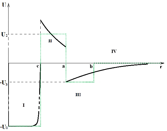
Figure 10: The approximation of rectangular well for potential of OHe-nucleus system.

Solutions of Schrodinger equation for each of the four regions, indicated on Fig. 10, are given in textbooks (see e.g.mk1rLL3 ) and their sewing determines the condition, under which a low-energy OHe-nucleus bound state appears in the region III.

0.31.3 Low energy bound state of O-helium with nuclei

The energy of this bound state and its existence strongly depend on the parameters $\mu$ and $g^{2}$ of nuclear potential (361). On the Fig. 11 the regions of these parameters, giving 4 keV energy level in OHe bound state with sodium are presented. Radiative capture to this level can explain results of DAMA/NaI and DAMA/LIBRA experiments with the account for their energy resolution mk1rDAMAlibra . The lower shaded region on Fig. 11 corresponds to the case of nuclear Yukawa potential $U_{3m}$, averaged over the orbit of He in OHe, while the upper region corresponds to the case of nuclear Yukawa potential $U_{3b}$ with the position of He most close to the nucleus at $\rho=r_{o}$.The result is also sensitive to the precise value of $d_{o}$, which determines the size of nuclei $R=d_{o}A^{1/3}$. The two narrow strips in each region correspond to the experimentally most probable value $d_{o}=1.2/(200\,{\rm MeV})$. In these calculations the mass of OHe was taken equal to $m_{o}=1TeV$, however the results weakly depend on the value of $m_{o}>1TeV$.

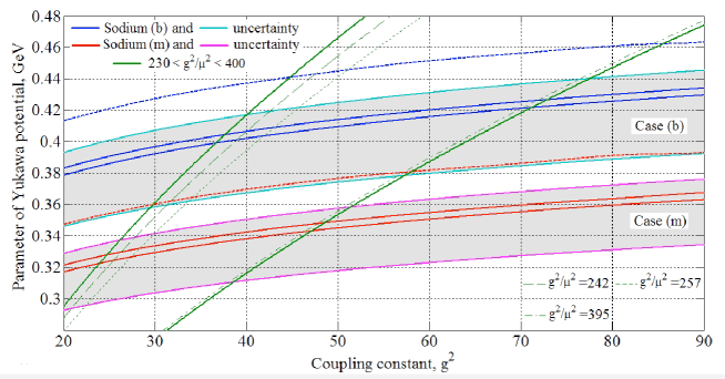
Figure 11: The region of parameters $\mu$ and $g^{2}$, for which Na-OHe system has a level in the interval 4 keV. Two lines determine at $d_{o}=1.2/(200\,{\rm MeV})$ the region of parameters, at which the bound system of this element with OHe has a 4 keV level. In the region between the two strips the energy of level is below 4 keV. There are also indicated the range of $g^{2}/\mu^{2}$ (dashed lines) as well as their preferred values (thin lines) determined in mk1rnuclear from parametrization of the relativistic ($\sigma-\omega$) model for nuclear matter. The uncertainty in the determination of parameter $1.15/(200\,{\rm MeV})<d_{o}<1.3/(200\,{\rm MeV})$ results in the uncertainty of $\mu$ and $g^{2}$ shown by the shaded regions surrounding the lines. The case of nuclear Yukawa potential $U_{3m}$, averaged over the orbit of He in OHe, corresponds to the lower lines and shaded region, while the upper lines and shaded region around them illustrate the case of nuclear Yukawa potential $U_{3b}$ with the position of He most close to the nucleus at $\rho=r_{o}$.

It is interesting that the values of $\mu$ on Fig. 11 are compatible with the results of recent experimental measurements of mass of sigma meson mk1rsigma .

0.31.4 Energy levels in other nuclei

The important qualitative feature of the presented solution is the restricted range of intermediate nuclei, in which the OHe-nucleus state beyond nuclei is possible. For the chosen range of nuclear parameters, reproducing the results of DAMA/NaI and DAMA/LIBRA, we can calculate the binding energy of OHe-nucleus states in nuclei, corresponding to chemical composition of set-ups in other experiments. It turns out that there are no such states for light and heavy nuclei. In the case of nuclear Yukawa potential $U_{3b}$, corresponding to the position of He most close to the nucleus at $\rho=r_{o}$, the range of nuclei with bound states with OHe corresponds to the part of periodic table between B and Ti. This result is stable independent on the used scheme of numerical calculations. The upper limits on the nuclear parameters $\mu$ and $g^{2}$, at which there exists OHe-nucleus bound state are presented for this case on Fig.12. In the case of potential $U_{3m}$, averaged over the orbit of He in OHe, there are no OHe bound states with nuclei, lighter than Be and heavier than Ti. However, the results are very sensitive to the numerical factors of calculations and the existence of OHe-Ge and OHe-Ga bound states at a narrow window of parameters $\mu$ and $g^{2}$ turns to be strongly dependent on these factors so that change in numbers smaller than 1% can give qualitatively different result for Ge and Ga. The results for the case (m) are shown on Fig.13.

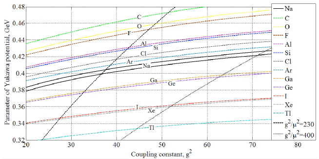
Figure 12: Existence of low energy bound states in OHe-nucleus system in the case b for nuclear Yukawa potential $U_{3b}$ with the position of He most close to the nucleus at $\rho=r_{o}$. The lines, corresponding to different nuclei, show the upper limit for nuclear physics parameters $\mu$ and $g^{2}$, at which these bound states are possible. The choice of parameters corresponding to 4 keV OHe-Na bound state, excludes region below Na line.

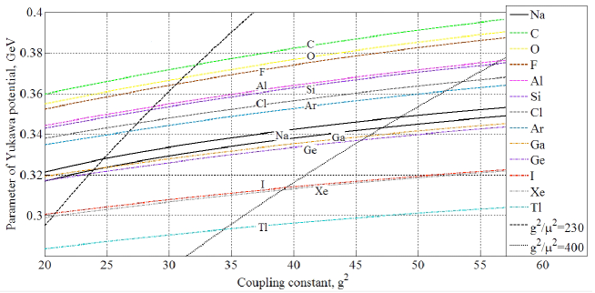
Figure 13: Existence of low energy bound states in OHe-nucleus system in the case m for nuclear Yukawa potential $U_{3m}$, averaged over the orbit of He in OHe. The lines, corresponding to different nuclei, show the upper limit for nuclear physics parameters $\mu$ and $g^{2}$, at which these bound states are possible. The choice of parameters corresponding to 4 keV OHe-Na bound state, excludes region below Na line.

Both for the cases (b) and (m) there is a stable conclusion that there are no OHe-nucleus bound states with Xe, I and Tl.

For the experimentally preferred value $d_{o}=1.2/(200\,{\rm MeV})$ the results of calculation of the binding energy of OHe-nucleus systems for carbon, oxygen, fluorine, argon, silicon, aluminium and chlorine are presented on Fig. 14 for the case of the nuclear Yukawa potential $U_{3b}$ and on Fig. 15 for the case of the potential $U_{3m}$. The difference in these results demonstrates their high sensitivity to the choice of parameters.

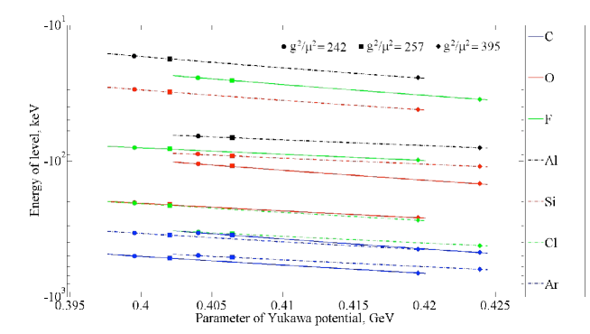
Figure 14: Energy levels in OHe bound system with carbon, oxygen, fluorine, argon, silicon, aluminium and chlorine for the case of the nuclear Yukawa potential $U_{3b}$. The predictions are given for the range of $g^{2}/\mu^{2}$ determined in mk1rnuclear from parametrization of the relativistic ($\sigma-\omega$) model for nuclear matter. The preferred values of $g^{2}/\mu^{2}$ are indicated by the corresponding marks (squares or circles).

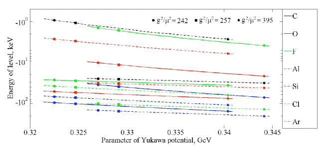
Figure 15: Energy levels in OHe bound system with carbon, oxygen, fluorine, argon, silicon, aluminium and chlorine for the case of the nuclear Yukawa potential $U_{3m}$. The predictions are given for the range of $g^{2}/\mu^{2}$ determined in mk1rnuclear from parametrization of the relativistic ($\sigma-\omega$) model for nuclear matter. The preferred values of $g^{2}/\mu^{2}$ are indicated by the corresponding marks (squares or circles).

0.32 Conclusions

To conclude, the results of dark matter search in experiments DAMA/NaI and DAMA/LIBRA can be explained in the framework of composite dark matter scenario without contradiction with negative results of other groups. This scenario can be realized in different frameworks, in particular in Minimal Walking Technicolor model or in the approach unifying spin and charges and contains distinct features, by which the present explanation can be distinguished from other recent approaches to this problem mk1rEdward (see also review and more references in mk1rGelmini ).

Our explanation is based on the mechanism of low energy binding of OHe with nuclei. We have found that within the uncertainty of nuclear physics parameters there exists their range at which OHe binding energy with sodium is equal to 4 keV and there is no such binding with iodine and thallium.

With the account for high sensitivity of our results to the values of uncertain nuclear parameters and for the approximations, made in our calculations, the presented results can be considered only as an illustration of the possibility to explain effects in underground detectors by OHe binding with intermediate nuclei. However, even at the present level of our studies we can make a conclusion that effects of such binding should strongly differ in detectors with the content, different from NaI, and can be absent in detectors with very light (e.g. ${}^{3}He$) and heavy nuclei (like xenon and probably germanium). Therefore test of results of DAMA/NaI and DAMA/LIBRA experiments by other experimental groups can become a very nontrivial task.

Can the Matter-Antimatter Asymmetry be Easier to Understand Within the ”Spin-charge-family-theory”, Predicting Twice Four Families and Two Times $SU(2)$ Vector Gauge and Scalar Fields? N.S. Mankoč Borštnik

0.33 Introduction

The theory unifying spin and charges and predicting families (spin-charge-family-theory) assumes that spinors carry in $d\geq 4$ ($d=1+13$ is studied) only two kinds of the spin. The Dirac kind $\gamma^{a}$ manifests after several appropriate breaks of the starting symmetry as the spin and all the charges. The second kind called $\{\gamma^{a}$ ($\{\gamma^{a},\tilde{\gamma}^{b}\}_{+}=0$) generates families. Accordingly there are in $d\geq 4$, besides the vielbeins, also the two kinds of the spin connection fields, which are the gauge fields of the corresponding operators $S^{ab}$ and $\tilde{S}^{ab}$. Those connected with $S^{ab}$ manifest in $d=(1+3)$ as the vector gauge fields, while those connected with $\tilde{S}^{ab}$ manifest as the scalar fields and determine on the tree level the mass matrices.

Let me make a short review of the so far made predictions of the spin-charge-family-theory:

• The spin-charge-family-theory has the explanation for the appearance of the internal degrees of freedom – the spin and the charges while unifying them under the assumption that the universe went through several phase transitions which cause the appropriate breaks of the starting symmetry. Then the fact that the right handed (with respect to SO(1,3)) fermions are weak chargeless, while the left handed ones carry the weak charge emerges, as well as that there exist leptons (singlets with respect to the colour charge) and quarks (triplets with respect to the colour charge) snmb2bnorma ; snmb2bpikanorma .

• The theory explains the appearance of massless families at the low energy regime under the assumption that there are breaks which leave the massless fermions of only one handedness snmb2bhnd . Assuming that breaks of symmetries affect the whole internal space — the space defined by both kinds of the Clifford algebra objects — it predicts in the energy regime close below $10^{16}$ GeV eight massless families. The manifested symmetry is (assumed to be) at this stage $SO(1,3)\times SO(4)\times U(1)\times SU(3)$. The next break of the symmetry of the universe to $SO(1,3)\times SU(2)\times U(1)\times SU(3)$ leaves four families massless snmb2bpikanorma , while the vacuum expectation values of superposition of the starting fields which manifest in $(1+3)$ as scalar fields, make the upper four families and the corresponding gauge fields massive. After the electroweak break also the lower four families become massive due to the vacuum expectation values of superposition of the starting fields, together with the weak bosons.

• The theory predicts the fourth family, which will be observed at the LHC or at somewhat higher energies snmb2bgmdn , and the fifth stable family (with no mixing matrix elements couplings to the lower four families in comparison with the age of the universe), the baryons and neutrinos of which are the candidates to form the dark matter.

• The masses of this fifth family members are according to the so far made rough estimations snmb2bpikanorma ; snmb2bgmdn larger than a few TeV and smaller than $10^{10}$ TeV. The members of the family have approximately the same mass, at least on the tree level snmb2bnormaproc2010talk .

• The studies snmb2bgn of the history of the stable fifth family members in the evolution of the universe and of their interactions with the ordinary matter in the DAMA s and the CDMS s experiments done so far lead to the prediction that the masses of the fifth family members, if they constitute the dark matter, are a few hundred TeV, independent of the fifth family fermion-antifermion asymmetry. The Xe experiment looks like to be in disagreement, but careful analyses show that one should wait for further data snmb2bdiscussGN to make the final conclusion.

  The lightest fifth family baryon is, in the case that all the quarks have approximately (within a hundred GeV) the same mass snmb2bgn , the fifth family neutron, due to the attractive electromagnetic interaction. The difference in the weak interaction can be for large enough masses neglected.

• The fermion asymmetry in the approach has not yet really been studied.

• The studies snmb2bgn of the evolution of this stable fifth family members rely on my rough estimations snmb2bgn of the behaviour of the coloured fifth family objects (single quarks and antiquarks or coloured pairs of quarks or of antiquarks) during the colour phase transition. These estimations namely suggest that the coloured objects either annihilate with the anti-objects or they form colourless neutrons and antineutrons and correspondingly decouple from the plasma soon after the colour phase transition starts, due to the very strong binding energy of the fifth family baryons (with respect to the first family baryons) long enough before the first family quarks start to form the baryons. These estimations should be followed by more accurate studies.

• The so far done studies suggest strongly that the number density of the fifth family neutrinos (of approximately the same mass as the fifth family quarks and leptons), which also contribute to the dark matter, is pretty much reduced due to the neutrino-antineutrino annihilation closed below the electroweak break. The weak annihilation cross section is expected to play much stronger role for neutrinos than for strongly bound fifth family quarks in the fifth family neutron (due to the huge binding energy of the fifth family quarks), what also remains to be proved.

• The estimations snmb2bgmdn of the properties of the lower four families on the tree level call for the calculations beyond the tree level, which should hopefully demonstrate, that the loop corrections (in all orders) bring the main differences in the properties of the family members. These calculations are in progress snmb2bAN .

Although we can say that the spin-charge-family-theory looks very promising as the right way to explain where do the assumptions of the standard model originate, there are obviously many not yet studied, or at least far from being carefully enough studied open problems. Many a problem is common to all the theories, like the first family baryon asymmetry, which I am going to discuss within the spin-charge-family-theory in this contribution. Some of the problems are common to all the theories assuming more than so far observed $(1+3)$ dimensions, in particular the spin-charge-family-theory shares some problems with all the Kaluza-Klein-like theories. We are trying to solve them first on toy models snmb2bhnd .

The main new step in the spin-charge-family-theory — the explanation of the appearance of families by assuming that both existing kinds of the Clifford algebra objects should be used to treat correctly the fermion degrees of freedom — limits very much the properties of families and their members. The simple starting action in $d=(1+13)$, which in $d=(1+3)$ demonstrates the mass matrices, namely fixes to high extent the fermion properties after the breaks of symmetries. Therefore this proposal might soon be studied accurately enough to show whether it is the right theory or not.

This contribution is an attempt to try to understand what can the spin-charge-family-theory say about the fermion-antifermion asymmetry when taking into account the proposals of the references snmb2brubakovshaposhnikov ; snmb2bdinekusenko ; snmb2btapeiling (and of the works cited therein). These works study the soliton solutions of non Abelian gauge fields with many different vacua and evaluate fermion number nonconservation due to possible transitions among different vacua in non equilibrium processes during the phase transitions through which the universe passed. In such processes fermion (and also antifermion) currents are not conserved since $CP$ is not nonconserved. To the $CP$ nonconservation also the complex matrix elements determining the transitions among families contribute and consequently influence the first family fermion-antifermion asymmetry.

Since the spin-charge-family-theory predicts below the unification scale of all the charges two kinds of phase transitions (first from $SO(1,3)\times SU(2)\times SU(2)\times U(1)\times SU(3)$ to $SO(1,3)\times SU(2)\times U(1)\times SU(3)$, in which the upper four families gain masses and so do the corresponding vector gauge fields, and then from $SO(1,3)\times SU(2)\times U(1)\times SU(3)$ to $SO(1,3)\times U(1)\times SU(3)$, in which the lower four families and the corresponding gauge fields gain masses), in which besides the vector gauge fields also the scalar gauge fields (the gauge fields of $\tilde{S}^{ab}$ and also of $S^{ab}$ with the scalar index with respect to $(1+3)$) contribute, the fermion-antifermion asymmetry might very probably have for the stable fifth family an opposite sign than for the first family.

It might therefore be that the existence of two kinds of four families, together with two kinds of the vector gauge fields and two kinds of the scalar fields help to easier understanding the first family fermion-antifermion asymmetry.

Although I am studying the fermion asymmetry, together with the discrete symmetries, in the spin-charge-family-theory for quite some time (not really intensively), this contribution is stimulated by the question of M.Y. Khlopov snmb2bMYN , since he is proposing the scenario, in which my stable fifth family members should manifest an opposite fermion asymmetry than the first family members, that is antifermion-fermion asymmetry. While in the case that the fifth family members have masses around 100 TeV or higher and the neutron is the lightest baryon and neutrino the lightest lepton snmb2bgn the fifth family baryon asymmetry plays no role (since in this case the fifth family neutrons and neutrinos as well as their antiparticles interact weakly enough among themselves and with the ordinary matter that the assumption that they constitute the dark matter is in agreement with the observations). Maxim snmb2bm claims that the fifth family members with the quark masses not higher than 10 TeV are also the candidates for the dark matter, provided that $\bar{u}_{5}\bar{u}_{5}\bar{u}_{5}$ is the lightest antibaryon and that there is an excess of antibaryons over the baryons in the fifth family case.

0.34 A short overview of the theory unifying spin and charges and explaining families

In this section I briefly repeat the main ideas of the spin-charge-family-theory. I kindly ask the reader to learn more about this theory in the references snmb2bnorma ; snmb2bpikanorma as well as in my talk presented in this proceedings and in the references therein.

I am proposing a simple action in $d=(1+13)$-dimensional space. Spinors carry two kinds of the spin (no charges).
i. The Dirac spin, described by $\gamma^{a}$’s, defines the spinor representation in $d=(1+13)$. After the break of the starting symmetry $SO(1,13)$ (through $SO(1,7)\times SO(6)$) to the symmetry of the standard model in $d=(1+3)$ ($SO(1,3)\times U(1)\times SU(2)\times SU(3)$) it defines the hyper charge ($U(1)$), the weak charge ($SU(2)$, with the left handed representation of $SO(1,3)$ manifesting naturally the weak charge and the right handed ones appearing as the weak singlets) and the colour charge ($SU(3)$).
ii. The second kind of the spin snmb2bnorma , described by $\tilde{\gamma}^{a}$’s ($\{\tilde{\gamma}^{a},\tilde{\gamma}^{b}\}_{+}=2\,\eta^{ab}$) and anticommuting with the Dirac $\gamma^{a}$ ($\{\gamma^{a},\tilde{\gamma}^{b}\}_{+}=0$), defines the families of spinors.
Accordingly spinors interact with the two kinds of the spin connection fields and the vielbeins.

We have

$$\{\gamma^{a},\gamma^{b}\}_{+}=2\eta^{ab}=\{\tilde{\gamma}^{a},\tilde{\gamma}^{b}\}_{+},\quad\{\gamma^{a},\tilde{\gamma}^{b}\}_{+}=0,$$

$$S^{ab}:=(i/4)(\gamma^{a}\gamma^{b}-\gamma^{b}\gamma^{a}),\quad\tilde{S}^{ab}:=(i/4)(\tilde{\gamma}^{a}\tilde{\gamma}^{b}-\tilde{\gamma}^{b}\tilde{\gamma}^{a}),\quad\{S^{ab},\tilde{S}^{cd}\}_{-}=0.$$

(364)

The action

$$S\, = \int\;d^{d}x\;E\;{\mathcal{L}}_{f}+$$ (365)

$$\int\;d^{d}x\;E\;(\alpha\,R+\tilde{\alpha}\,\tilde{R})\,,$$

$${\mathcal{L}}_{f} = \frac{1}{2}\,(E\bar{\psi}\,\gamma^{a}p_{0a}\psi)+h.c.\,,$$

$$p_{0a} = f^{\alpha}{}_{a}p_{0\alpha}+\frac{1}{2E}\,\{p_{\alpha},Ef^{\alpha}{}_{a}\}_{-},$$

$$p_{0\alpha} = p_{\alpha}-\frac{1}{2}S^{ab}\omega_{ab\alpha}-\frac{1}{2}\tilde{S}^{ab}\tilde{\omega}_{ab\alpha}\,,$$

$$R = \frac{1}{2}\,\{f^{\alpha[a}f^{\beta b]}\;(\omega_{ab\alpha,\beta}-\omega_{ca\alpha}\,\omega^{c}{}_{b\beta})\}+h.c.\;,$$

$$\tilde{R} = \frac{1}{2}\,f^{\alpha[a}f^{\beta b]}\;(\tilde{\omega}_{ab\alpha,\beta}-\tilde{\omega}_{ca\alpha}\tilde{\omega}^{c}{}_{b\beta})+h.c.\;,$$ (366)

manifests ($f^{\alpha[a}f^{\beta b]}=f^{\alpha a}f^{\beta b}-f^{\alpha b}f^{\beta a}$) after the break of symmetries all the known gauge fields and the scalar fields, and the mass matrices. To see the manifestation of the covariant momentum and the mass matrices we rewrite formally the action for a Weyl spinor in $d=(1+13)$ as follows

$${\mathcal{L}}_{f} = \bar{\psi}\gamma^{m}(p_{m}-\sum_{A,i}\;g^{A}\tau^{Ai}A^{Ai}_{m})\psi+$$ (367)

$$\{\sum_{s=7,8}\;\bar{\psi}\gamma^{s}p_{0s}\;\psi\}+$$

$${\rm the\;rest},$$

where $m=0,1,2,3$ with

$$\tau^{Ai}=\sum_{a,b}\;c^{Ai}{}_{ab}\;S^{ab},$$

$$\{\tau^{Ai},\tau^{Bj}\}_{-}=i\delta^{AB}f^{Aijk}\tau^{Ak}.$$ (368)

All the charges and the spin of one family are determined by $S^{ab}$, with $S^{ab}$ as the only internal degree of freedom of one family (besides the family quantum number, determined by $\tilde{S}^{ab}$), manifesting after the breaks at the low energy regime as the generators of the observed groups (Eq. (368)) $U(1),SU(2)$ and $SU(3)$, for $A=1,2,3$, respectively.

The breaks of the starting symmetry from $SO(1,13)$ to the symmetry $SO(1,7)\times SU(3)\times U(1)$ and further to $SO(1,3)\times SU(2)\times SU(2)\times U(1)\times SU(3)$ are assumed to leave all the low lying families of spinors massless. There are eight such massless families ($2^{8/2-1}$) before further breaks.

Accordingly the first row of the action in Eq. (367) manifests the effective standard model fermions part of the action before the weak break, while the second part manifests, after the appropriate breaks of symmetries (when $\omega_{ab\sigma}$ and $\tilde{\omega}_{ab\sigma}$, $\sigma\in(5,6,7,8),$ fields gain the nonzero vacuum expectation values on the tree level) the mass matrices.

The generators $\tilde{S}^{ab}$ take care of the families, transforming each member of one family into the corresponding member of another family, due to the fact that $\{S^{ab},\tilde{S}^{cd}\}_{-}=0$ (Eq.(364)).

Using the technique snmb2bsnmb:hn02hn03 and analysing the vectors as the eigenvectors of the standard model groups we present vectors in the space of charges and spins in terms of projectors and nilpotents as can be learned in Appendix, in the references snmb2bnorma ; snmb2bpikanorma and also in my talk in the Proceedings of Bled workshop 2010.

I present in Table 1 the eightplet (the representation of $SO(1,7)$ of quarks of a particular colour charge ($\tau^{33}=1/2$, $\tau^{38}=1/(2\sqrt{3})$), and $U(1)$ charge ($\tau^{4}=1/6$) and on Table 2 the eightplet of the corresponding (colour chargeless) leptons.

i		$|^{a}\psi_{i}>$	$\Gamma^{(1,3)}$	$S^{12}$	$\Gamma^{(4)}$	$\tau^{13}$	$\tau^{23}$	$Y$	$Q$
		${\rm Octet},\;\Gamma^{(1,7)}=1,\;\Gamma^{(6)}=-1,$
		${\rm of\;quarks}$
1	$u_{R}^{c1}$	$\stackrel{{\scriptstyle 03}}{{(+i)}}\,\stackrel{{\scriptstyle 12}}{{(+)}}|\stackrel{{\scriptstyle 56}}{{(+)}}\,\stackrel{{\scriptstyle 78}}{{(+)}}||\stackrel{{\scriptstyle 9\;10}}{{(+)}}\;\;\stackrel{{\scriptstyle 11\;12}}{{[-]}}\;\;\stackrel{{\scriptstyle 13\;14}}{{[-]}}$	1	$\frac{1}{2}$	1	0	$\frac{1}{2}$	$\frac{2}{3}$	$\frac{2}{3}$
2	$u_{R}^{c1}$	$\stackrel{{\scriptstyle 03}}{{[-i]}}\,\stackrel{{\scriptstyle 12}}{{[-]}}|\stackrel{{\scriptstyle 56}}{{(+)}}\,\stackrel{{\scriptstyle 78}}{{(+)}}||\stackrel{{\scriptstyle 9\;10}}{{(+)}}\;\;\stackrel{{\scriptstyle 11\;12}}{{[-]}}\;\;\stackrel{{\scriptstyle 13\;14}}{{[-]}}$	1	$-\frac{1}{2}$	1	0	$\frac{1}{2}$	$\frac{2}{3}$	$\frac{2}{3}$
3	$d_{R}^{c1}$	$\stackrel{{\scriptstyle 03}}{{(+i)}}\,\stackrel{{\scriptstyle 12}}{{(+)}}|\stackrel{{\scriptstyle 56}}{{[-]}}\,\stackrel{{\scriptstyle 78}}{{[-]}}||\stackrel{{\scriptstyle 9\;10}}{{(+)}}\;\;\stackrel{{\scriptstyle 11\;12}}{{[-]}}\;\;\stackrel{{\scriptstyle 13\;14}}{{[-]}}$	1	$\frac{1}{2}$	1	0	$-\frac{1}{2}$	$-\frac{1}{3}$	$-\frac{1}{3}$
4	$d_{R}^{c1}$	$\stackrel{{\scriptstyle 03}}{{[-i]}}\,\stackrel{{\scriptstyle 12}}{{[-]}}|\stackrel{{\scriptstyle 56}}{{[-]}}\,\stackrel{{\scriptstyle 78}}{{[-]}}||\stackrel{{\scriptstyle 9\;10}}{{(+)}}\;\;\stackrel{{\scriptstyle 11\;12}}{{[-]}}\;\;\stackrel{{\scriptstyle 13\;14}}{{[-]}}$	1	$-\frac{1}{2}$	1	0	$-\frac{1}{2}$	$-\frac{1}{3}$	$-\frac{1}{3}$
5	$d_{L}^{c1}$	$\stackrel{{\scriptstyle 03}}{{[-i]}}\,\stackrel{{\scriptstyle 12}}{{(+)}}|\stackrel{{\scriptstyle 56}}{{[-]}}\,\stackrel{{\scriptstyle 78}}{{(+)}}||\stackrel{{\scriptstyle 9\;10}}{{(+)}}\;\;\stackrel{{\scriptstyle 11\;12}}{{[-]}}\;\;\stackrel{{\scriptstyle 13\;14}}{{[-]}}$	-1	$\frac{1}{2}$	-1	$-\frac{1}{2}$	0	$\frac{1}{6}$	$-\frac{1}{3}$
6	$d_{L}^{c1}$	$\stackrel{{\scriptstyle 03}}{{(+i)}}\,\stackrel{{\scriptstyle 12}}{{[-]}}|\stackrel{{\scriptstyle 56}}{{[-]}}\,\stackrel{{\scriptstyle 78}}{{(+)}}||\stackrel{{\scriptstyle 9\;10}}{{(+)}}\;\;\stackrel{{\scriptstyle 11\;12}}{{[-]}}\;\;\stackrel{{\scriptstyle 13\;14}}{{[-]}}$	-1	$-\frac{1}{2}$	-1	$-\frac{1}{2}$	0	$\frac{1}{6}$	$-\frac{1}{3}$
7	$u_{L}^{c1}$	$\stackrel{{\scriptstyle 03}}{{[-i]}}\,\stackrel{{\scriptstyle 12}}{{(+)}}|\stackrel{{\scriptstyle 56}}{{(+)}}\,\stackrel{{\scriptstyle 78}}{{[-]}}||\stackrel{{\scriptstyle 9\;10}}{{(+)}}\;\;\stackrel{{\scriptstyle 11\;12}}{{[-]}}\;\;\stackrel{{\scriptstyle 13\;14}}{{[-]}}$	-1	$\frac{1}{2}$	-1	$\frac{1}{2}$	0	$\frac{1}{6}$	$\frac{2}{3}$
8	$u_{L}^{c1}$	$\stackrel{{\scriptstyle 03}}{{(+i)}}\,\stackrel{{\scriptstyle 12}}{{[-]}}|\stackrel{{\scriptstyle 56}}{{(+)}}\,\stackrel{{\scriptstyle 78}}{{[-]}}||\stackrel{{\scriptstyle 9\;10}}{{(+)}}\;\;\stackrel{{\scriptstyle 11\;12}}{{[-]}}\;\;\stackrel{{\scriptstyle 13\;14}}{{[-]}}$	-1	$-\frac{1}{2}$	-1	$\frac{1}{2}$	0	$\frac{1}{6}$	$\frac{2}{3}$

Table 1: The 8-plet of quarks - the members of $SO(1,7)$ subgroup of the group $SO(1,13)$, belonging to one Weyl left handed ($\Gamma^{(1,13)}=-1=\Gamma^{(1,7)}\times\Gamma^{(6)}$) spinor representation of $SO(1,13)$. It contains the left handed weak charged quarks and the right handed weak chargeless quarks of a particular colour $(1/2,1/(2\sqrt{3}))$. Here $\Gamma^{(1,3)}$ defines the handedness in $(1+3)$ space, $S^{12}$ defines the ordinary spin (which can also be read directly from the basic vector, both vectors with both spins, $\pm\frac{1}{2}$, are presented), $\tau^{13}$ defines the third component of the weak charge, $\tau^{23}$ the third component of the $SU(2)_{II}$ charge, $\tau^{4}$ (the $U(1)$ charge) defines together with the $\tau^{23}$ the hyper charge ($Y=\tau^{4}+\tau^{23}$), $Q=Y+\tau^{13}$ is the electromagnetic charge. The reader can find the whole Weyl representation in the ref. snmb2bPortoroz03 .

i		$|^{a}\psi_{i}>$	$\Gamma^{(1,3)}$	$S^{12}$	$\Gamma^{(4)}$	$\tau^{13}$	$\tau^{23}$	$Y$	$Q$
		${\rm Octet},\;\Gamma^{(1,7)}=1,\;\Gamma^{(6)}=-1,$
		${\rm of\;quarks}$
1	$\nu_{R}$	$\stackrel{{\scriptstyle 03}}{{(+i)}}\,\stackrel{{\scriptstyle 12}}{{(+)}}|\stackrel{{\scriptstyle 56}}{{(+)}}\,\stackrel{{\scriptstyle 78}}{{(+)}}||\stackrel{{\scriptstyle 9\;10}}{{(+)}}\;\;\stackrel{{\scriptstyle 11\;12}}{{(+)}}\;\;\stackrel{{\scriptstyle 13\;14}}{{(+)}}$	1	$\frac{1}{2}$	1	0	$\frac{1}{2}$	$0$	$0$
2	$\nu_{R}$	$\stackrel{{\scriptstyle 03}}{{[-i]}}\,\stackrel{{\scriptstyle 12}}{{[-]}}|\stackrel{{\scriptstyle 56}}{{(+)}}\,\stackrel{{\scriptstyle 78}}{{(+)}}||\stackrel{{\scriptstyle 9\;10}}{{(+)}}\;\;\stackrel{{\scriptstyle 11\;12}}{{[-]}}\;\;\stackrel{{\scriptstyle 13\;14}}{{[-]}}$	1	$-\frac{1}{2}$	1	0	$\frac{1}{2}$	$0$	$0$
3	$e_{R}$	$\stackrel{{\scriptstyle 03}}{{(+i)}}\,\stackrel{{\scriptstyle 12}}{{(+)}}|\stackrel{{\scriptstyle 56}}{{[-]}}\,\stackrel{{\scriptstyle 78}}{{[-]}}||\stackrel{{\scriptstyle 9\;10}}{{(+)}}\;\;\stackrel{{\scriptstyle 11\;12}}{{[-]}}\;\;\stackrel{{\scriptstyle 13\;14}}{{[-]}}$	1	$\frac{1}{2}$	1	0	$-\frac{1}{2}$	$-1$	$-1$
4	$e_{R}$	$\stackrel{{\scriptstyle 03}}{{[-i]}}\,\stackrel{{\scriptstyle 12}}{{[-]}}|\stackrel{{\scriptstyle 56}}{{[-]}}\,\stackrel{{\scriptstyle 78}}{{[-]}}||\stackrel{{\scriptstyle 9\;10}}{{(+)}}\;\;\stackrel{{\scriptstyle 11\;12}}{{[-]}}\;\;\stackrel{{\scriptstyle 13\;14}}{{[-]}}$	1	$-\frac{1}{2}$	1	0	$-\frac{1}{2}$	$-1$	$-1$
5	$e_{L}$	$\stackrel{{\scriptstyle 03}}{{[-i]}}\,\stackrel{{\scriptstyle 12}}{{(+)}}|\stackrel{{\scriptstyle 56}}{{[-]}}\,\stackrel{{\scriptstyle 78}}{{(+)}}||\stackrel{{\scriptstyle 9\;10}}{{(+)}}\;\;\stackrel{{\scriptstyle 11\;12}}{{[-]}}\;\;\stackrel{{\scriptstyle 13\;14}}{{[-]}}$	-1	$\frac{1}{2}$	-1	$-\frac{1}{2}$	0	$-\frac{1}{2}$	$-1$
6	$e_{L}$	$\stackrel{{\scriptstyle 03}}{{(+i)}}\,\stackrel{{\scriptstyle 12}}{{[-]}}|\stackrel{{\scriptstyle 56}}{{[-]}}\,\stackrel{{\scriptstyle 78}}{{(+)}}||\stackrel{{\scriptstyle 9\;10}}{{(+)}}\;\;\stackrel{{\scriptstyle 11\;12}}{{[-]}}\;\;\stackrel{{\scriptstyle 13\;14}}{{[-]}}$	-1	$-\frac{1}{2}$	-1	$-\frac{1}{2}$	0	$-\frac{1}{2}$	$-1$
7	$\nu_{L}$	$\stackrel{{\scriptstyle 03}}{{[-i]}}\,\stackrel{{\scriptstyle 12}}{{(+)}}|\stackrel{{\scriptstyle 56}}{{(+)}}\,\stackrel{{\scriptstyle 78}}{{[-]}}||\stackrel{{\scriptstyle 9\;10}}{{(+)}}\;\;\stackrel{{\scriptstyle 11\;12}}{{[-]}}\;\;\stackrel{{\scriptstyle 13\;14}}{{[-]}}$	-1	$\frac{1}{2}$	-1	$\frac{1}{2}$	0	$-\frac{1}{2}$	$0$
8	$\nu_{L}$	$\stackrel{{\scriptstyle 03}}{{(+i)}}\,\stackrel{{\scriptstyle 12}}{{[-]}}|\stackrel{{\scriptstyle 56}}{{(+)}}\,\stackrel{{\scriptstyle 78}}{{[-]}}||\stackrel{{\scriptstyle 9\;10}}{{(+)}}\;\;\stackrel{{\scriptstyle 11\;12}}{{[-]}}\;\;\stackrel{{\scriptstyle 13\;14}}{{[-]}}$	-1	$-\frac{1}{2}$	-1	$\frac{1}{2}$	0	$-\frac{1}{2}$	$0$

Table 2: The 8-plet of leptons - the members of $SO(1,7)$ subgroup of the group $SO(1,13)$, belonging to one Weyl left handed ($\Gamma^{(1,13)}=-1=\Gamma^{(1,7)}\times\Gamma^{(6)}$) spinor representation of $SO(1,13)$. It contains the colour chargeless left handed weak charged leptons and the right handed weak chargeless leptons. The rest of notation is the same as in Table 2.

In both tables the vectors are chosen to be the eigenvectors of the operators of handedness $\Gamma^{(n)}$, the generators $\tau^{13},\,\tau^{23},\,\tau^{33}$ $\tau^{38}$, $Y=\tau^{4}+\tau^{23}$ and $Q=Y+\tau^{13}$. They are also eigenvectors of the corresponding $\tilde{S}^{ab}$, $\tilde{\tau}^{Ai},A=1,2,3$ and $\tilde{Y},\tilde{Q}$. One easily sees that the right handed vectors (with respect to $SO(1,3)$ ) are weak ($SU(2)_{I}$) chargeless and are doublets with respect to the second $SU(2)_{II}$, while the left handed are weak charged and singlets with respect to $SU(2)_{II}$.

The generators $\tilde{S}^{ab}$ transform each member of a family into the same member of other $2^{\frac{8}{2}-1}$ families. The eight families of the first member of the eightplet of quarks from Table 1, for example, that is of the right handed $u$-quark of the spin $\frac{1}{2}$, are presented in the left column of Table 3. The corresponding right handed neutrinos, belonging to eight different families, are presented in the right column of the same table. The $u$-quark member of the eight families and the $\nu$ members of the same eight families are generated by $\tilde{S}^{cd}$, $c,d\in\{0,1,2,3,5,6,7,8\}$ from any starting family.

$I_{R}$	$u_{R}^{c1}$	$\stackrel{{\scriptstyle 03}}{{[+i]}}\,\stackrel{{\scriptstyle 12}}{{(+)}}|\stackrel{{\scriptstyle 56}}{{(+)}}\,\stackrel{{\scriptstyle 78}}{{[+]}}||\stackrel{{\scriptstyle 9\;10}}{{(+)}}\>\;\stackrel{{\scriptstyle 11\;12}}{{[-]}}\;\;\stackrel{{\scriptstyle 13\;14}}{{[-]}}$	$\nu_{R}$	$\stackrel{{\scriptstyle 03}}{{[+i]}}\,\stackrel{{\scriptstyle 12}}{{(+)}}|\stackrel{{\scriptstyle 56}}{{(+)}}\,\stackrel{{\scriptstyle 78}}{{[+]}}||\stackrel{{\scriptstyle 9\;10}}{{(+)}}\;\;\stackrel{{\scriptstyle 11\;12}}{{(+)}}\;\;\stackrel{{\scriptstyle 13\;14}}{{(+)}}$
$II_{R}$	$u_{R}^{c1}$	$\stackrel{{\scriptstyle 03}}{{[+i]}}\,\stackrel{{\scriptstyle 12}}{{(+)}}|\stackrel{{\scriptstyle 56}}{{[+]}}\,\stackrel{{\scriptstyle 78}}{{(+)}}||\stackrel{{\scriptstyle 9\;10}}{{(+)}}\;\;\stackrel{{\scriptstyle 11\;12}}{{[-]}}\;\;\stackrel{{\scriptstyle 13\;14}}{{[-]}}$	$\nu_{R}$	$\stackrel{{\scriptstyle 03}}{{(+i)}}\,\stackrel{{\scriptstyle 12}}{{[+]}}|\stackrel{{\scriptstyle 56}}{{(+)}}\,\stackrel{{\scriptstyle 78}}{{[+]}}||\stackrel{{\scriptstyle 9\;10}}{{(+)}}\;\;\stackrel{{\scriptstyle 11\;12}}{{(+)}}\;\;\stackrel{{\scriptstyle 13\;14}}{{(+)}}$
$III_{R}$	$u_{R}^{c1}$	$\stackrel{{\scriptstyle 03}}{{(+i)}}\,\stackrel{{\scriptstyle 12}}{{[+]}}|\stackrel{{\scriptstyle 56}}{{(+)}}\,\stackrel{{\scriptstyle 78}}{{[+]}}||\stackrel{{\scriptstyle 9\;10}}{{(+)}}\;\;\stackrel{{\scriptstyle 11\;12}}{{[-]}}\;\;\stackrel{{\scriptstyle 13\;14}}{{[-]}}$	$\nu_{R}$	$\stackrel{{\scriptstyle 03}}{{(+i)}}\,\stackrel{{\scriptstyle 12}}{{[+]}}|\stackrel{{\scriptstyle 56}}{{[+]}}\,\stackrel{{\scriptstyle 78}}{{(+)}}||\stackrel{{\scriptstyle 9\;10}}{{(+)}}\;\;\stackrel{{\scriptstyle 11\;12}}{{(+)}}\;\;\stackrel{{\scriptstyle 13\;14}}{{(+)}}$
$IV_{R}$	$u_{R}^{c1}$	$\stackrel{{\scriptstyle 03}}{{(+i)}}\,\stackrel{{\scriptstyle 12}}{{[+]}}|\stackrel{{\scriptstyle 56}}{{[+]}}\,\stackrel{{\scriptstyle 78}}{{(+)}}||\stackrel{{\scriptstyle 9\;10}}{{(+)}}\;\;\stackrel{{\scriptstyle 11\;12}}{{[-]}}\;\;\stackrel{{\scriptstyle 13\;14}}{{[-]}}$	$\nu_{R}$	$\stackrel{{\scriptstyle 03}}{{[+i]}}\,\stackrel{{\scriptstyle 12}}{{(+)}}|\stackrel{{\scriptstyle 56}}{{[+]}}\,\stackrel{{\scriptstyle 78}}{{(+)}}||\stackrel{{\scriptstyle 9\;10}}{{(+)}}\;\;\stackrel{{\scriptstyle 11\;12}}{{(+)}}\;\;\stackrel{{\scriptstyle 13\;14}}{{(+)}}$
$V_{R}$	$u_{R}^{c1}$	$\stackrel{{\scriptstyle 03}}{{(+i)}}\,\stackrel{{\scriptstyle 12}}{{(+)}}|\stackrel{{\scriptstyle 56}}{{(+)}}\,\stackrel{{\scriptstyle 78}}{{(+)}}||\stackrel{{\scriptstyle 9\;10}}{{(+)}}\;\;\stackrel{{\scriptstyle 11\;12}}{{[-]}}\;\;\stackrel{{\scriptstyle 13\;14}}{{[-]}}$	$\nu_{R}$	$\stackrel{{\scriptstyle 03}}{{(+i)}}\,\stackrel{{\scriptstyle 12}}{{(+)}}|\stackrel{{\scriptstyle 56}}{{(+)}}\,\stackrel{{\scriptstyle 78}}{{(+)}}||\stackrel{{\scriptstyle 9\;10}}{{(+)}}\;\;\stackrel{{\scriptstyle 11\;12}}{{(+)}}\;\;\stackrel{{\scriptstyle 13\;14}}{{(+)}}$
$VI_{R}$	$u_{R}^{c1}$	$\stackrel{{\scriptstyle 03}}{{(+i)}}\,\stackrel{{\scriptstyle 12}}{{(+)}}|\stackrel{{\scriptstyle 56}}{{[+]}}\,\stackrel{{\scriptstyle 78}}{{[+]}}||\stackrel{{\scriptstyle 9\;10}}{{(+)}}\;\;\stackrel{{\scriptstyle 11\;12}}{{[-]}}\;\;\stackrel{{\scriptstyle 13\;14}}{{[-]}}$	$\nu_{R}$	$\stackrel{{\scriptstyle 03}}{{(+i)}}\,\stackrel{{\scriptstyle 12}}{{(+)}}|\stackrel{{\scriptstyle 56}}{{[+]}}\,\stackrel{{\scriptstyle 78}}{{[+]}}||\stackrel{{\scriptstyle 9\;10}}{{(+)}}\;\;\stackrel{{\scriptstyle 11\;12}}{{(+)}}\;\;\stackrel{{\scriptstyle 13\;14}}{{(+)}}$
$VII_{R}$	$u_{R}^{c1}$	$\stackrel{{\scriptstyle 03}}{{[+i]}}\,\stackrel{{\scriptstyle 12}}{{[+]}}|\stackrel{{\scriptstyle 56}}{{(+)}}\,\stackrel{{\scriptstyle 78}}{{(+)}}||\stackrel{{\scriptstyle 9\;10}}{{(+)}}\;\;\stackrel{{\scriptstyle 11\;12}}{{[-]}}\;\;\stackrel{{\scriptstyle 13\;14}}{{[-]}}$	$\nu_{R}$	$\stackrel{{\scriptstyle 03}}{{[+i]}}\,\stackrel{{\scriptstyle 12}}{{[+]}}|\stackrel{{\scriptstyle 56}}{{(+)}}\,\stackrel{{\scriptstyle 78}}{{(+)}}||\stackrel{{\scriptstyle 9\;10}}{{(+)}}\;\;\stackrel{{\scriptstyle 11\;12}}{{(+)}}\;\;\stackrel{{\scriptstyle 13\;14}}{{(+)}}$
$VIII_{R}$	$u_{R}^{c1}$	$\stackrel{{\scriptstyle 03}}{{[+i]}}\,\stackrel{{\scriptstyle 12}}{{[+]}}|\stackrel{{\scriptstyle 56}}{{[+]}}\,\stackrel{{\scriptstyle 78}}{{[+]}}||\stackrel{{\scriptstyle 9\;10}}{{(+)}}\;\;\stackrel{{\scriptstyle 11\;12}}{{[-]}}\;\;\stackrel{{\scriptstyle 13\;14}}{{[-]}}$	$\nu_{R}$	$\stackrel{{\scriptstyle 03}}{{[+i]}}\,\stackrel{{\scriptstyle 12}}{{[+]}}|\stackrel{{\scriptstyle 56}}{{[+]}}\,\stackrel{{\scriptstyle 78}}{{[+]}}||\stackrel{{\scriptstyle 9\;10}}{{(+)}}\;\;\stackrel{{\scriptstyle 11\;12}}{{(+)}}\;\;\stackrel{{\scriptstyle 13\;14}}{{(+)}}$

Table 3: Eight families of the right handed $u_{R}$ quark with the spin $\frac{1}{2}$, the colour charge $\tau^{33}=1/2$, $\tau^{38}=1/(2\sqrt{3})$ and of the colourless right handed neutrino $\nu_{R}$ of the spin $\frac{1}{2}$ are presented in the left and in the right column, respectively. $S^{ab},a,b\in\{0,1,2,3,5,6,7,8\}$ transform $u_{R}^{c1}$ of the spin $\frac{1}{2}$ and the chosen colour $c1$ to all the members of the same colour: to the right handed $u_{R}^{c1}$ of the spin $-\frac{1}{2}$, to the left $u_{L}^{c1}$ of both spins ($\pm\frac{1}{2}$), to the right handed $d_{R}^{c1}$ of both spins ($\pm\frac{1}{2}$) and to the left handed $d_{L}^{c1}$ of both spins ($\pm\frac{1}{2}$). They transform equivalently the right handed neutrino $\nu_{R}$ of the spin $\frac{1}{2}$ to the right handed $\nu_{R}$ of the spin ($-\frac{1}{2}$), to $\nu_{L}$ of both spins, to $e_{R}$ of both spins and to $e_{L}$ of both spins. $\tilde{S}^{ab},a,b\in\{0,1,2,3,5,6,7,8\}$ transform a chosen member of one family into the same member of all the eight families.

Let us present also the quantum numbers of the families from Table 3. In Table 4 the handedness of the families $\tilde{\Gamma}^{(1+3)}(=-4i\tilde{S}^{03}\tilde{S}^{12})$, $\tilde{S}^{03}_{L},\tilde{S}^{12}_{L}$, $\tilde{S}^{03}_{R},\tilde{S}^{12}_{R}$ (the diagonal matrices of $SO(1,3)$ ), $\tilde{\tau}^{13}$ (of one of the two $SU(2)_{I}$), $\tilde{\tau}^{23}$ (of the second $SU(2)_{II}$) are presented.

$i$	$\tilde{\Gamma}^{(1+3)}$	$\tilde{S}^{03}_{L}$	$\tilde{S}^{12}_{L}$	$\tilde{S}^{03}_{R}$	$\tilde{S}^{12}_{R}$	$\tilde{\tau}^{13}$	$\tilde{\tau}^{23}$	$\tilde{\tau}^{4}$	$\tilde{Y}^{\prime}$	$\tilde{Y}$	$\tilde{Q}$
$1$	$-1$	$-\frac{i}{2}$	$\frac{1}{2}$	$0$	$0$	$\frac{1}{2}$	$0$	$-\frac{1}{2}$	$0$	$-\frac{1}{2}$	$0$
$2$	$-1$	$-\frac{i}{2}$	$\frac{1}{2}$	$0$	$0$	$-\frac{1}{2}$	$0$	$-\frac{1}{2}$	$0$	$-\frac{1}{2}$	$-1$
$3$	$-1$	$\frac{i}{2}$	$-\frac{1}{2}$	$0$	$0$	$\frac{1}{2}$	$0$	$-\frac{1}{2}$	$0$	$-\frac{1}{2}$	$0$
$4$	$-1$	$\frac{i}{2}$	$-\frac{1}{2}$	$0$	$0$	$-\frac{1}{2}$	$0$	$-\frac{1}{2}$	$0$	$-\frac{1}{2}$	$-1$
$5$	$1$	$0$	$0$	$\frac{i}{2}$	$\frac{1}{2}$	$0$	$\frac{1}{2}$	$-\frac{1}{2}$	$\frac{1}{2}$	$0$	$0$
$6$	$1$	$0$	$0$	$\frac{i}{2}$	$\frac{1}{2}$	$0$	$-\frac{1}{2}$	$-\frac{1}{2}$	$-\frac{1}{2}$	$-1$	$-1$
$7$	$1$	$0$	$0$	$-\frac{i}{2}$	$-\frac{1}{2}$	$0$	$\frac{1}{2}$	$-\frac{1}{2}$	$\frac{1}{2}$	$0$	$0$
$8$	$1$	$0$	$0$	$-\frac{i}{2}$	$-\frac{1}{2}$	$0$	$-\frac{1}{2}$	$-\frac{1}{2}$	$-\frac{1}{2}$	$-1$	$-1$

Table 4: The quantum numbers of each member of the eight families presented in Table 3 are presented: The handedness of the families $\tilde{\Gamma}^{(1+3)}=-4i\tilde{S}^{03}\tilde{S}^{12}$, the left and right handed $SO(1,3)$ quantum numbers $\tilde{S}^{03}_{L},\tilde{S}^{12}_{L}$, $\tilde{S}^{03}_{R},\tilde{S}^{12}_{R}$ (of $SO(1,3)$ group in the $\tilde{S}^{mn}$ sector), $\tilde{\tau}^{13}$ of $SU(2)_{I}$, $\tilde{\tau}^{23}$ of the second $SU(2)_{II}$, $\tilde{\tau}^{4}$, $\tilde{Y}^{\prime}=\tilde{\tau}^{23}-\tilde{\tau}^{4}\,\tan\tilde{\theta}_{2}$, taking $\tilde{\theta}^{2}=0$, $\tilde{Y}=\tilde{\tau}^{4}+\tilde{\tau}^{23}$, $\tilde{Q}=\tilde{\tau}^{4}+\tilde{S}^{56}$. See also the ref. snmb2bnormaproc2010talk .

We see in Table 4 that four of the eight families are singlets with respect to one of the two $SU(2)$ ($SU(2)_{I}$) groups determined by $\tilde{S}^{ab}$ and doublets with respect to the second $SU(2)$ ($SU(2)_{II}$), while the remaining four families are doublets with respect to the first $SU(2)_{I}$ and singlets with respect to the second $SU(2)_{II}$. When the first break appears, to which besides the vielbeins also the spin connections contribute, we expect that if only one of the two $SU(2)$ subgroups of $SO(1,7)\times U(1)$ breaking into $SO(1,3)\times SU(2)\times U(1)$ contributes in the break snmb2bnormaproc2010talk , namely that of the charges $\tilde{\tau}^{2i}$, together with $\tilde{N}^{i}_{-}$, there will be four families massless and mass protected after this break, namely those, which are singlets with respect to $\mathchoice{\mbox{\boldmath$\displaystyle\tilde{\tau}$}}{\mbox{\boldmath$\textstyle\tilde{\tau}$}}{\mbox{\boldmath$\scriptstyle\tilde{\tau}$}}{\mbox{\boldmath$\scriptscriptstyle\tilde{\tau}$}}^{2}$ and with respect to $\tilde{N}^{i}_{-}$ (Table 4), while for the other four families the vacuum expectation values of the scalars (particular combinations of vielbeins $f^{\sigma}{}_{s}$, and spin connections $\tilde{\omega}_{abs},s\in\{5,8\}$) will take care of the mass matrices on the tree level and beyond the tree level.

0.34.1 Discrete symmetries of the theory unifying spin and charges and explaining families

Let us define the discrete operators of the parity ($P$) and of the charge conjugation ($C$).

$$P = \gamma^{0}\,\gamma^{8}\,I_{x}\,,$$

$$C = \Pi_{Im\,\gamma^{a}}\,\gamma^{a}\,K\,.$$ (369)

$K$ means complex conjugation, while in our choice of matrix representation of the $\gamma^{a}$ matrices $\Pi_{Im\,\gamma^{a}}\,\gamma^{a}\,=\gamma^{2}\gamma^{5}\gamma^{7}\gamma^{9}\gamma^{11}\gamma^{13}$.

One can easily check that $P$ transforms the $u_{R}^{c1}$ from the first row in Table 1 into the $u_{L}^{c1}$ of the seventh row in the same table. The $CP$ transforms the fermion states of table 1 into the corresponding states of antifermions: $u_{R}^{c1}$ from the first row in table 1 with the spin $\frac{1}{2}$, weak chargeless and of the colour charge ($(\frac{1}{2},\frac{1}{2\sqrt{3}})$) into a right handed antiquark $\bar{u}_{R}^{\bar{c1}}$, weak charged and of the colour charge ($(-\frac{1}{2},-\frac{1}{2\sqrt{3}})$) as presented in table 5.

i		$|^{a}\psi_{i}>$	$\Gamma^{(1,3)}$	$S^{12}$	$\Gamma^{(4)}$	$\tau^{13}$	$\tau^{23}$	$Y$	$Q$
		${\rm Octet},\;\Gamma^{(1,7)}=-1,\;\Gamma^{(6)}=1,$
		${\rm of\;antiquarks}$
1	$\bar{u}_{R}^{\bar{c1}}$	$\stackrel{{\scriptstyle 03}}{{[-i]}}\,\stackrel{{\scriptstyle 12}}{{[-]}}|\stackrel{{\scriptstyle 56}}{{[-]}}\,\stackrel{{\scriptstyle 78}}{{(+)}}||\stackrel{{\scriptstyle 9\;10}}{{[-]}}\;\;\stackrel{{\scriptstyle 11\;12}}{{(+)}}\;\;\stackrel{{\scriptstyle 13\;14}}{{(+)}}$	1	$-\frac{1}{2}$	-1	$-\frac{1}{2}$	$0$	$-\frac{1}{6}$	$-\frac{2}{3}$
2	$\bar{u}_{R}^{\bar{c1}}$	$\stackrel{{\scriptstyle 03}}{{(+i)}}\,\stackrel{{\scriptstyle 12}}{{(+)}}|\stackrel{{\scriptstyle 56}}{{[-]}}\,\stackrel{{\scriptstyle 78}}{{(+)}}||\stackrel{{\scriptstyle 9\;10}}{{[-]}}\;\;\stackrel{{\scriptstyle 11\;12}}{{(+)}}\;\;\stackrel{{\scriptstyle 13\;14}}{{(+)}}$	1	$\frac{1}{2}$	-1	$-\frac{1}{2}$	$0$	$-\frac{1}{6}$	$-\frac{2}{3}$
3	$\bar{d}_{R}^{\bar{c1}}$	$\stackrel{{\scriptstyle 03}}{{[-i]}}\,\stackrel{{\scriptstyle 12}}{{[-]}}|\stackrel{{\scriptstyle 56}}{{(+)}}\,\stackrel{{\scriptstyle 78}}{{[-]}}||\stackrel{{\scriptstyle 9\;10}}{{[-]}}\;\;\stackrel{{\scriptstyle 11\;12}}{{(+)}}\;\;\stackrel{{\scriptstyle 13\;14}}{{(+)}}$	1	$-\frac{1}{2}$	-1	$\frac{1}{2}$	$0$	$-\frac{1}{6}$	$\frac{1}{3}$
4	$\bar{d}_{R}^{\bar{c1}}$	$\stackrel{{\scriptstyle 03}}{{(+i)}}\,\stackrel{{\scriptstyle 12}}{{(+)}}|\stackrel{{\scriptstyle 56}}{{(+)}}\,\stackrel{{\scriptstyle 78}}{{[-]}}||\stackrel{{\scriptstyle 9\;10}}{{[-]}}\;\;\stackrel{{\scriptstyle 11\;12}}{{(+)}}\;\;\stackrel{{\scriptstyle 13\;14}}{{(+)}}$	1	$\frac{1}{2}$	-1	$\frac{1}{2}$	$0$	$-\frac{1}{6}$	$\frac{1}{3}$
5	$\bar{d}_{L}^{\bar{c1}}$	$\stackrel{{\scriptstyle 03}}{{(+i)}}\,\stackrel{{\scriptstyle 12}}{{[-]}}|\stackrel{{\scriptstyle 56}}{{(+)}}\,\stackrel{{\scriptstyle 78}}{{(+)}}||\stackrel{{\scriptstyle 9\;10}}{{[-]}}\;\;\stackrel{{\scriptstyle 11\;12}}{{(+)}}\;\;\stackrel{{\scriptstyle 13\;14}}{{(+)}}$	-1	$-\frac{1}{2}$	1	$0$	$\frac{1}{2}$	$\frac{1}{3}$	$\frac{1}{3}$
6	$\bar{d}_{L}^{\bar{c1}}$	$\stackrel{{\scriptstyle 03}}{{[-i])}}\,\stackrel{{\scriptstyle 12}}{{(+)}}|\stackrel{{\scriptstyle 56}}{{(+)}}\,\stackrel{{\scriptstyle 78}}{{(+)}}||\stackrel{{\scriptstyle 9\;10}}{{[-]}}\;\;\stackrel{{\scriptstyle 11\;12}}{{(+)}}\;\;\stackrel{{\scriptstyle 13\;14}}{{(+)}}$	-1	$\frac{1}{2}$	1	$0$	$\frac{1}{2}$	$\frac{1}{3}$	$\frac{1}{3}$
7	$\bar{u}_{L}^{\bar{c1}}$	$\stackrel{{\scriptstyle 03}}{{(+i)}}\,\stackrel{{\scriptstyle 12}}{{[-]}}|\stackrel{{\scriptstyle 56}}{{[-]}}\,\stackrel{{\scriptstyle 78}}{{[-]}}||\stackrel{{\scriptstyle 9\;10}}{{[-]}}\;\;\stackrel{{\scriptstyle 11\;12}}{{(+)}}\;\;\stackrel{{\scriptstyle 13\;14}}{{(+)}}$	-1	$-\frac{1}{2}$	1	$0$	$-\frac{1}{2}$	$-\frac{2}{3}$	$-\frac{2}{3}$
8	$\bar{u}_{L}^{\bar{c1}}$	$\stackrel{{\scriptstyle 03}}{{[-i]}}\,\stackrel{{\scriptstyle 12}}{{(+)}}|\stackrel{{\scriptstyle 56}}{{[-]}}\,\stackrel{{\scriptstyle 78}}{{[-]}}||\stackrel{{\scriptstyle 9\;10}}{{[-]}}\;\;\stackrel{{\scriptstyle 11\;12}}{{(+)}}\;\;\stackrel{{\scriptstyle 13\;14}}{{(+)}}$	-1	$\frac{1}{2}$	1	$0$	$-\frac{1}{2}$	$-\frac{2}{3}$	$-\frac{2}{3}$

Table 5: The 8-plet of antiquarks to the quarks obtained from Table 1 by the $CP$ ($=\gamma^{2}\gamma^{5}\gamma^{7}\gamma^{9}\gamma^{11}\gamma^{13}K\gamma^{0}\gamma^{8}\,I_{x}$) conjugation.

0.35 The fermion-antifermion asymmetry within the theory unifying spin and charges and explaining families

As said in the abstract, I shall here follow the ideas from the references snmb2bgross ; snmb2brubakovshaposhnikov ; snmb2bdinekusenko ; snmb2btapeiling . The difference from the studies there in here is, as explained, in the number of families (there are two decoupled groups of four families and consequently two stable families), in the number of gauge fields contributing to the phase transitions and in the types of the gauge fields contributing to phase transitions.

Let us assume that the fermion-antifermion asymmetry is zero, when the expanding universe cools down to the temperature below the unification scale of the spin and the charges that is to the temperature below, let say, $10^{16}$ TeV, when there are eight massless families, manifesting the symmetry $SO(1,3)\times SU(2)\times SU(2)\times U(1)\times SU(3)$, and distinguishing among themselves in the quantum numbers defined by $\tilde{S}^{ab}$.

Then we must investigate, how much do the following processes contribute to the fermion-antifermion asymmetry in non equilibrium thermal processes in the expanding universe:

• The nonconservation of currents on the quantum level due to the triangle anomalies snmb2btapeiling ; snmb2brubakovshaposhnikov ; snmb2bdinekusenko , which are responsible for $P$ and $CP$ nonconservation

  $$\partial^{m}\,j^{Ai\,\alpha(i)}_{m} = \frac{(g^{A})^{2}}{8\pi^{2}}\;\frac{1}{2}\,\varepsilon_{mnpr}\,F^{Ai\,mn}F^{Ai\,pr}.$$ (370)

  Here $j^{Ai\,\alpha}_{m}$ stays for the currents of fermions (and antifermions), which carry a particular charge denoted by a charge group $A$, in our case $A=4$ means the $U(1)$ charge originating in $SO(6)$, $A=3$ means the $SU(3)$ (colour) charge, $A=2_{I}$ means the weak $SU(2)_{I}$ charge of the left handed doublets, while $A=2_{II}$ stays for the $SU(2)_{II}$ charge of the right handed singlets before the $SU(2)_{II}$ break, $A=1$ stays for the actual $U(1)$ charge (the standard model like hyper charge after the $SU(2)_{II}$ break and the electromagnetic one after the weak break).

  In my case also the fields, which look like scalar fields in $d=(1+3)$, $\tilde{A}^{\tilde{A}i}_{s}$, $s,t\in{5,6,\cdots}$, and to which the fermions are coupled, contribute.

  All the fermions and antifermions, which are coupled to a particular gauge field $A^{Ai}_{m}$ and in my case also $\tilde{A}^{\tilde{A}i}_{s}$ contribute to the current

  $$j^{Ai\,\alpha(i)}_{m}=\psi^{Ai\,\alpha(i)\dagger}\,\gamma^{0}\gamma^{m}\,\psi^{Ai\,\alpha(i)}.$$ (371)

  $(i)\in\{1,8\}$ enumerates families, in my case twice four families which are distinguishable by the quantum numbers originating in $\tilde{S}^{ab}$, namely, after the break of $SU(2)_{I}$ the lower four families, which are doublets with respect to $\tilde{N}^{i}_{+}$ and $\tilde{\tau}^{I\,i}$ and singlets with respect to $\tilde{N}^{i}_{-}$ and $\tilde{\tau}^{II\,i}$, stay massless, while the upper four families are doublets with respect to $\tilde{N}^{i}_{-}$ and $\tilde{\tau}^{IIi}$ and singlets with respect to $\tilde{N}^{i}_{+}$ and $\tilde{\tau}^{Ii}$. After the electroweak break all the eight families become massive, but the upper four families have no mixing matrix elements since the way of breaking leaves all the $\omega_{msa}$ and $\tilde{\omega}_{msa}$, with $m=0,1,2,3;s=5,6,\cdots$, equal to zero. $\alpha$ distinguishes the multiplets in each family, in my case of the two $SU(2)$ gauge groups $\alpha$ distinguishes the $SU(2)_{I}$ doublets, that is one colour singlet and one colour triplet, and the $SU(2)_{II}$ doublets, again one colour singlet and one colour triplet. $A^{Ai}_{m}$ are the corresponding gauge fields, with tensors $F^{A}_{mn}=\tau^{Ai}\,F^{Ai}_{mn}$ and $F^{Ai}_{mn}=A^{Ai}_{n,m}-A^{Ai}_{m,n}+g^{A}\,f^{Aijk}\,A^{Aj}_{m}\,A^{Ak}_{n}$. (The scalar fields $\tilde{A}^{\tilde{A}i}_{s}$ define tensors $\tilde{F}^{\tilde{A}i\,st}=\tilde{A}^{\tilde{A}i}_{t,s}-\tilde{A}^{\tilde{A}i}_{s,t}+g^{\tilde{}A}\,f^{A\,ijk}\tilde{A}^{\tilde{A}j}_{s}\,\tilde{A}^{\tilde{A}k}_{t}$.)

  The nonconserved currents affect the fermions and antifermions. (In the later case the $\tau^{Ai}$ are replaced by $\bar{\tau}^{Ai}$, both fulfilling the same commutation relations $\{\tau^{Ai},\tau^{Bj}\}_{-}=i\delta^{AB}\,f^{A\,ijk}\,\tau^{Ak}$, $\{\bar{\tau}^{Ai},\bar{\tau}^{Bj}\}_{-}=i\delta^{AB}\,f^{A\,ijk}\,\bar{\tau}^{Ak}$). One obtains $\bar{\tau}^{Ai}$ from $\tau^{Ai}$ by the $CP$ transformation $P=\gamma^{0}\gamma^{8}\,I_{x}$, while $C=\prod_{Im\gamma^{a}}\,\gamma^{a}\,K$ (See 0.34.1).

• The nonconservation of the fermion numbers originating in the complex phases of the mixing matrices of the two times $4\times 4$ mass matrices for each member of a family, after the two successive breaks causes two phase transitions when the symmetry $SU(2)\times SU(2)\times U(1)$ breaks first to $SU(2)\times U(1)$ and finally to $U(1)$ and the two types of gauge fields manifest their masses while the two groups of four with the mixing matrices decoupled families gain nonzero mass matrices in the first break the upper four families and in the second break the lower four families.

I am following here the references snmb2bgross ; snmb2brubakovshaposhnikov ; snmb2bdinekusenko ; snmb2btapeiling . The nonconservation of currents may be expected whenever the non-Abelian gauge fields manifest a non trivial structure of vacua, originating in the instanton solutions of the Euclidean non-Abelian gauge theories in $(1+3)-$dimensional space, that is in $A^{A}_{m}$, which fulfil the boundary condition $\lim_{r\to\infty}\;\tau^{Ai}\,A^{Ai}_{m}=U^{-1}\partial_{m}U$, summed over $i$ for a particular gauge group $A$ (and similarly might be that the fields $\lim_{\rho\to\infty}\;\tilde{\tau}^{\tilde{A}i}\,\tilde{A}^{\tilde{A}i}_{s}=U^{-1}\partial_{s}U$, with $r=\sqrt{(x^{0})^{2}+\mathchoice{\mbox{\boldmath$\displaystyle x$}}{\mbox{\boldmath$\textstyle x$}}{\mbox{\boldmath$\scriptstyle x$}}{\mbox{\boldmath$\scriptscriptstyle x$}}^{2}}$ and $\rho=\sqrt{\sum_{s}}\,(x^{s})^{2}$, for a particular $\tilde{A}$ , contribute as well, where the effect of the triangle anomalies in the case of scalar gauge fields depending on $x^{\sigma},\sigma=5,6,7,8$ and the corresponding meaning of the winding numbers distinguishing among the different vacua in this case might be negligible and should be studied). The vacua distinguish among themselves in the topological quantum numbers $n_{A}$ ($n_{\tilde{A}}$), determined by a particular choice of $U$

$$n_{A}=\frac{(g^{A})^{2}}{16\pi^{2}}\,\int d^{4}x\,\varepsilon_{mnpr}\,Tr(F^{Amn}F^{Apr})=\frac{(g^{A})^{2}}{32\pi^{2}}\,\int d^{4}x\partial_{m}K^{A\,m},$$ (372)

where $K^{A}_{m}=\sum_{i}4\varepsilon_{mnpr}\,(A^{Ai}_{n}\partial_{p}A^{A}_{r}+\frac{2}{3}\,g^{A}f^{Aijk}A^{Ai}_{n}A^{Aj}_{p}A^{Ak}_{r}).$ (Similarly also the topological quantum number $n_{\tilde{A}}$ might be non negligible.)

Instanton solutions fulfilling the boundary condition $\lim_{r\to\infty}\;\tau^{Ai}\,A^{Ai}_{m}=U^{-1}\partial_{m}U$ for a particular gauge group $A$ (or $\lim_{\rho\to\infty}\;\tilde{\tau}^{\tilde{A}i}\,\tilde{A}^{\tilde{A}i}_{s}=U^{-1}\partial_{m}U$ for a particular $\tilde{A}$), each with its own $U$ for a particular $A$ (or $\tilde{A}$), connect vacua $|n_{A}>$ with different winding numbers  $n_{A}$ (and correspondingly for $n_{\tilde{A}}$). The true vacuum $|\theta^{A}>$ is for each $A$ (let it count also $\tilde{A}$) in a stationary situation a superposition of the vacua, determined by the time independent gauge transformation snmb2bgross ${\cal T}$, ${\cal T}|\theta^{A}>=e^{i\theta^{A}}|\theta^{A}>$, where $\theta^{A}$ is a parameter, which weights the contribution of a vacuum to the effective Lagrange density ${\cal L}_{eff}={\cal L}+\sum_{A}\,\frac{\theta^{A}}{16\pi^{2}}\,F^{Ai\,mn}\frac{1}{2}\varepsilon_{mnpr}F^{Ai\,pr}$, for a particular gauge field. ${\cal T}$ acts as the raising operator for the handedness (chirality). The second term of the effective Lagrange density ${\cal L}_{eff}$ violates parity $P$ and then also $CP$. The vacuum state with the definite handedness has also a definite topological quantum number. In the presence of the massless fermions all the vacua $|\theta^{A}>$, for each $A$, are equivalent.

The fermion currents (Eq.(371)) are not conserved in processes, for which the gauge fields are such that the corresponding winding number $n_{A}$ of Eq. (372) is nonzero. Correspondingly also the fermion (and antifermion numbers), carrying the corresponding charge, are not conserved

$$\Delta n_{Ai\,\alpha(i)}=n_{A}.$$ (373)

The fermion number of all the fermions interacting with the same non-Abelian gauge field with nonzero winding number, either of a vector or of a scalar type (whose contribution should be studied and hopefully understood), changes in such processes for the same amount: Any member of a family, interacting with the particular field and therefore also the corresponding members of each family, either a quark or a lepton member of doublets, change for the same amount, before the breaks or after the breaks (in my case first from $SO(1,3)\times SU(2)\times SU(2)\times U(1)\times SU(3)$ to $SO(1,3)\times SU(2)\times U(1)\times SU(3)$ and finally to $SO(1,3)\times U(1)\times SU(3)$) of the symmetries.

For a baryon three quarks are needed. It is the conservation of the colour charge which requires that the lepton number and the baryon number ought to be conserved separately as long as the charge group is a global symmetry. The transformations, which allow rotations of a lepton to a quark or opposite, conserve the fermion number, but not the lepton and not the baryon number.

Instanton solutions of the non-Abelian gauge fields, which connect different vacua (see the refs. snmb2btapeiling , page 481, and snmb2brubakovshaposhnikov , page 6), are characterized by the highest value of the instanton field between the two vacua, that is by the sphaleron energy.

The question arises, can the instanton solutions be responsible for the baryon asymmetry of the universe? The authors of the papers snmb2brubakovshaposhnikov ; snmb2bdinekusenko discuss and evaluate the probability for tunnelling from one vacuum to the other at low energy regime and also at the energies of sphalerons. When once the system of gauge fields is in one vacuum the probability for the transition to another vacuum depends not only on the sphalerons height (energy) but also on the temperature. If the temperature is low, then the transition is negligible. At the temperature above the phase transition (the authors snmb2brubakovshaposhnikov discuss the electroweak phase transition starting at around $100$ GeV, while in my case there is also the $SU(2)_{II}$ phase transition at around $10^{16}$ GeV or slightly below) when the fermions are massless and the expansion rate of the universe is much slower that the rate of nonconservation of the fermion number, and in the case of non equilibrium processes in phase transitions, the fermion number nonconservation can be large. The authors conclude that more precise evaluations (treating several models) of the probability that in a non thermal equilibrium phase transition and below it the fermion number would not be conserved due to transitions to vacua with different winding numbers in the amount as observed for the (first family) baryon number excess in the universe are needed.

What can be concluded about the fermion number asymmetry, caused by the transitions of gauge fields to different vacua, in my case, where at energies above the $SU{2}_{II}$ phase transition there are eight families of massless fermions, with the charges manifesting the symmetries first of $SU(2)_{I}\times SU(2)_{II}\times U(1)$ and correspondingly with the two kinds of the vector gauge $SU(2)$ fields which both might demonstrate the vacua with different winding numbers? In addition also the scalar gauge fields might contribute with their even more rich vacua (if they do that at all). The phase transitions caused first by the break of the symmetry $SU(2)_{I}\times SU(2)_{II}\times U(1)$ to $SU(2)_{II}\times U(1)$, when the upper four families gain masses (and the corresponding gauge vector fields become massive) and then by the final break to $U(1)$, with the $\tilde{S}^{ab}$ sector causing the masses in both transitions and may be also taking care of the richness of vacua with different winding numbers, might show up after a careful study as a mechanism for generating the fermion-antifermion (or the antifermion-fermion) asymmetry. Although I do not yet see, how do the non equilibrium processes in the first order phase transitions decide about the excess of either fermions or of antifermions.

So, is it in my case possible that the two successive non equilibrium phase transitions leave the excess of antifermions in the case of the upper four families and the excess of fermions in the lower four families? Or there is a negligible excess of either fermions or antifermions in the upper four families? We saw in the ref. snmb2bgn that an excess of either fermions or antifermions is not important for massive enough (few $100$ TeV) stable fifth family members. The excess of fermions over antifermions is certainly what universe made a choice of for the lower four families, whatever the reason for this fact is. Can this be easier understood within the spin-charge-family-theory? All these need a careful study.

The fermion number nonconservation originates also in the complex phases of the mass mixing matrices of each of the two groups of four family members. It might be that the vacua, triggered by instanton solutions of the gauge vector and scalar fields, and the mass matrices, determined on the tree level by the vacuum expectation values of the scalar gauge fields in the $\tilde{S}^{ab}$ sector, are connected (since in the instanton case also the scalar fields, the gauge fields of charges originating in $\tilde{S}^{ab}$ might exhibit the instanton solutions).

0.36 Conclusion

In this contribution I pay attention to the origin of baryon asymmetry of our universe within the spin-charge-family-theory under the assumption that the asymmetry is caused i. by the instanton solutions of the non-Abelian gauge fields which determine vacua with different winding numbers and ii. by the complex matrix elements of the mixing matrices.

The spin-charge-family-theory namely assumes besides the Dirac Clifford algebra objects also the second ones $\tilde{\gamma^{a}}$ as a necessary mechanism (or better a mathematical tool) which should be used in order that we consistently describe both: spin and charges, as well as families. The second kind is namely responsible for generating families, defining the equivalent representations with respect to the Dirac one. Correspondingly there are besides the two kinds of the vector gauge fields, the $SU(2)_{I}$ and $SU(2)_{II}$, also the scalar gauge fields, the two $SU(2)$ from $SO(4)$ and the two $SU(2)$ from $SO(1,3)$, the superposition of the gauge fields of $\tilde{S}^{ab}(=\frac{i}{4}(\tilde{\gamma^{a}}\tilde{\gamma^{b}}-\tilde{\gamma^{b}}\tilde{\gamma^{a}}))$, which might contribute to vacua with different winding numbers (what has to be studied). The scalar fields, originating in the $\tilde{S}^{ab}$ charges, are responsible with their vacuum expectation values (and in loop corrections) for the mass matrices of fermions after the breaks of symmetries.

The theory predicts twice four families (which differ in the family quantum numbers in the way that the upper four families are doublets with respect to $\tilde{\tau}^{II\,i}$ and $\tilde{N}^{i}_{-}$, while the lower four families are doublets with respect to $\tilde{\tau}^{I\,i},$ and $\tilde{N}^{i}_{+}$) which all are massless above the last two phase transitions.

What should be clarified in the spin-charge-family-theory is whether the predicted twice four families (rather than once three families of the standard model) and the fact that there are gauge fields belonging to two kinds of generator ($S^{ab}$ and $\tilde{S}^{ab}$) make the baryon number asymmetry easier to be understood within these two phenomena — the instanton responsibility for the fermion number nonconservation and the complex matrix elements of the mixing matrices responsibility for the fermion number nonconservation.

The manifestation of the instanton gauge vector and scalar fields in the determination of the properties of the vacuum might be correlated with the vacuum expectation values of the scalar fields defining the mass matrices of twice the four families. Both manifestations appear in possibly non equilibrium phase transitions of the expanding universe, which cause breaking of particular symmetries and also the fermion number nonconservation. In this contribution I just follow the way suggested by the ref. snmb2brubakovshaposhnikov and by the authors cited in this reference, while taking into account the requirement of the spin-charge-family-theory. The fermion number nonconservation obviously ended in the excess of (what we call) fermions for the lower four families, while for the upper four families we have to see whether there is the excess of either the stable fifth family fermions or antifermions. To answer these questions a careful study is needed. It even might be that there was at the non equilibrium phase transitions the same excess of antifermions for the upper four families as it is of fermions for the lower four families, while later the complex matrix elements in the mixing matrices change this equality drastically. But yet it must be understood the origin of both sources of the fermion number nonconservation.

Appendix: Some useful relations

The following Cartan subalgebra set of the algebra $S^{ab}$ (for both sectors) is chosen:

$$S^{03},S^{12},S^{56},S^{78},S^{9\;10},S^{11\;12},S^{13\;14}$$

$$\tilde{S}^{03},\tilde{S}^{12},\tilde{S}^{56},\tilde{S}^{78},\tilde{S}^{9\;10},\tilde{S}^{11\;12},\tilde{S}^{13\;14}.$$ (374)

A left handed ($\Gamma^{(1,13)}=-1$) eigen state of all the members of the Cartan subalgebra

$$\stackrel{{\scriptstyle 03}}{{(+i)}}\stackrel{{\scriptstyle 12}}{{(+)}}|\stackrel{{\scriptstyle 56}}{{(+)}}\stackrel{{\scriptstyle 78}}{{(+)}}||\stackrel{{\scriptstyle 9\;10}}{{(+)}}\stackrel{{\scriptstyle 11\;12}}{{(-)}}\stackrel{{\scriptstyle 13\;14}}{{(-)}}|\psi\rangle=$$

$$\frac{1}{2^{7}}(\gamma^{0}-\gamma^{3})(\gamma^{1}+i\gamma^{2})|(\gamma^{5}+i\gamma^{6})(\gamma^{7}+i\gamma^{8})||$$

$$(\gamma^{9}+i\gamma^{10})(\gamma^{11}-i\gamma^{12})(\gamma^{13}-i\gamma^{14})|\psi\rangle.$$ (375)

represent the $u_{R}$-quark with spin up and of one colour.

$\tilde{S}^{ab}$ generate families from the starting $u_{R}$ quark In particular $\tilde{S}^{03}(=\frac{i}{2}[\stackrel{{\scriptstyle 03}}{{\tilde{(+i)}}}\stackrel{{\scriptstyle 12}}{{\tilde{(+)}}}+\stackrel{{\scriptstyle 03}}{{\tilde{(-i)}}}\stackrel{{\scriptstyle 12}}{{\tilde{(+)}}}+\stackrel{{\scriptstyle 03}}{{\tilde{(+i)}}}\stackrel{{\scriptstyle 12}}{{\tilde{(-)}}}+\stackrel{{\scriptstyle 03}}{{\tilde{(-i)}}}\stackrel{{\scriptstyle 12}}{{\tilde{(-)}}}])$ applied on a right handed $u_{R}$-quark with spin up and a particular colour generate a state which is again a right handed $u$-quark of the same colour.

$$\stackrel{{\scriptstyle 03}}{{\tilde{(-i)}}}\stackrel{{\scriptstyle 12}}{{\tilde{(-)}}} \stackrel{{\scriptstyle 03}}{{(+i)}}\stackrel{{\scriptstyle 12}}{{(+)}}|\stackrel{{\scriptstyle 56}}{{(+)}}\stackrel{{\scriptstyle 78}}{{(+)}}||\stackrel{{\scriptstyle 910}}{{(+)}}\stackrel{{\scriptstyle 1112}}{{(-)}}\stackrel{{\scriptstyle 1314}}{{(-)}}=$$ (376)

$$\stackrel{{\scriptstyle 03}}{{[\,+i]}}\stackrel{{\scriptstyle 12}}{{[\,+\,]}}|\stackrel{{\scriptstyle 56}}{{(+)}}\stackrel{{\scriptstyle 78}}{{(+)}}||\stackrel{{\scriptstyle 910}}{{(+)}}\stackrel{{\scriptstyle 1112}}{{(-)}}\stackrel{{\scriptstyle 1314}}{{(-)}},$$

where

$$\stackrel{{\scriptstyle ab}}{{(\pm i)}} = \frac{1}{2}\,(\gamma^{a}\mp\gamma^{b}),\stackrel{{\scriptstyle ab}}{{(\pm 1)}}=\frac{1}{2}\,(\gamma^{a}\pm i\gamma^{b}),$$

$$\stackrel{{\scriptstyle ab}}{{[\pm i]}} = \frac{1}{2}(1\pm\gamma^{a}\gamma^{b}),\quad\stackrel{{\scriptstyle ab}}{{[\pm 1]}}=\frac{1}{2}(1\pm i\gamma^{a}\gamma^{b}),$$

$$\stackrel{{\scriptstyle ab}}{{\tilde{(\pm i)}}} = \frac{1}{2}(\tilde{\gamma}^{a}\mp\tilde{\gamma}^{b}),\quad\stackrel{{\scriptstyle ab}}{{\tilde{(\pm 1)}}}=\frac{1}{2}(\tilde{\gamma}^{a}\pm i\tilde{\gamma}^{b}),$$

$$\stackrel{{\scriptstyle ab}}{{\tilde{[\pm i]}}} = \frac{1}{2}(1\pm\tilde{\gamma}^{a}\tilde{\gamma}^{b}),\quad\stackrel{{\scriptstyle ab}}{{\tilde{[\pm 1]}}}=\frac{1}{2}(1\pm i\tilde{\gamma}^{a}\tilde{\gamma}^{b}).$$ (377)

We present below some useful relations which are easy to derive snmb2bpikanorma .

$$\stackrel{{\scriptstyle ab}}{{(k)}}\stackrel{{\scriptstyle ab}}{{(k)}} = 0,\;\stackrel{{\scriptstyle ab}}{{(k)}}\stackrel{{\scriptstyle ab}}{{(-k)}}=\eta^{aa}\stackrel{{\scriptstyle ab}}{{[k]}},\;\stackrel{{\scriptstyle ab}}{{[k]}}\stackrel{{\scriptstyle ab}}{{[k]}}=\stackrel{{\scriptstyle ab}}{{[k]}},$$

$$\stackrel{{\scriptstyle ab}}{{[k]}}\stackrel{{\scriptstyle ab}}{{[-k]}} = 0,\stackrel{{\scriptstyle ab}}{{(k)}}\stackrel{{\scriptstyle ab}}{{[k]}}=0,\quad\;\stackrel{{\scriptstyle ab}}{{[k]}}\stackrel{{\scriptstyle ab}}{{(k)}}=\stackrel{{\scriptstyle ab}}{{(k)}},$$

$$\stackrel{{\scriptstyle ab}}{{(k)}}\stackrel{{\scriptstyle ab}}{{[-k]}} = \stackrel{{\scriptstyle ab}}{{(k)}}\,,\quad\;\stackrel{{\scriptstyle ab}}{{[k]}}\stackrel{{\scriptstyle ab}}{{(-k)}}=0.$$ (378)

$$\stackrel{{\scriptstyle ab}}{{\tilde{(k)}}}\stackrel{{\scriptstyle ab}}{{(k)}} = 0,\quad\;\stackrel{{\scriptstyle ab}}{{\tilde{(-k)}}}\stackrel{{\scriptstyle ab}}{{(k)}}=-i\eta^{aa}\stackrel{{\scriptstyle ab}}{{[k]}},$$

$$\stackrel{{\scriptstyle ab}}{{\tilde{(k)}}}\stackrel{{\scriptstyle ab}}{{[k]}} = i\stackrel{{\scriptstyle ab}}{{(k)}},\quad\stackrel{{\scriptstyle ab}}{{\tilde{(k)}}}\stackrel{{\scriptstyle ab}}{{[-k]}}=0.$$ (379)

$$N^{\pm}_{+} = N^{1}_{+}\pm i\,N^{2}_{+}=-\stackrel{{\scriptstyle 03}}{{(\mp i)}}\stackrel{{\scriptstyle 12}}{{(\pm)}}\,,\quad N^{\pm}_{-}=N^{1}_{-}\pm i\,N^{2}_{-}=\stackrel{{\scriptstyle 03}}{{(\pm i)}}\stackrel{{\scriptstyle 12}}{{(\pm)}}\,,$$

$$\tilde{N}^{\pm}_{+} = -\stackrel{{\scriptstyle 03}}{{\tilde{(\mp i)}}}\stackrel{{\scriptstyle 12}}{{\tilde{(\pm)}}}\,,\quad\tilde{N}^{\pm}_{-}=\stackrel{{\scriptstyle 03}}{{\tilde{(\pm i)}}}\stackrel{{\scriptstyle 12}}{{\tilde{(\pm)}}}\,,$$

$$\tau^{1\pm} = (\mp)\,\stackrel{{\scriptstyle 56}}{{(\pm)}}\stackrel{{\scriptstyle 78}}{{(\mp)}}\,,\quad\tau^{2\pm}=(\mp)\,\stackrel{{\scriptstyle 56}}{{(\mp)}}\stackrel{{\scriptstyle 78}}{{(\mp)}}\,,$$

$$\tilde{\tau}^{1\pm} = (\mp)\,\stackrel{{\scriptstyle 56}}{{\tilde{(\pm)}}}\stackrel{{\scriptstyle 78}}{{\tilde{(\mp)}}}\,,\quad\tilde{\tau}^{2\pm}=(\mp)\,\stackrel{{\scriptstyle 56}}{{\tilde{(\mp)}}}\stackrel{{\scriptstyle 78}}{{\tilde{(\mp)}}}\,.$$ (380)

Mass Matrices of Twice Four Families of Quarks
and Leptons, Scalars and Gauge Fields as Predicted by
the Spin-charge-family-theory On line lecture of N. S. M. B. available at
http://viavca.in2p3.fr/what_comes_beyond_the_standard_models_xiii.html N.S. Mankoč Borštnik

0.37 Introduction

The theory unifying spin and charges and predicting families snmb3tgnorma ; snmb3tgpikanorma ; snmb3tgnproc2007 ; snmb3tgdark2010 ; snmb3tggmdn ; snmb3tggn (to be called the spin-charge-family-theory) seems promising in explaining the assumptions of the standard model of the electroweak and colour interactions, in particular since it is proposing the mechanism for generating families. It assumes in $d=(1+(d-1))$, $d=14$, a simple starting action for spinors and the gauge fields: The spinors carry only two kinds of the spin (no charges), namely the one postulated by Dirac 80 years ago and the second kind proposed by the author of the paper (there is no third kind of the spin), and interact correspondingly with only the vielbeins and the two kinds of the spin connection fields. The action for the corresponding gauge fields contains the curvature in the first power for both kinds of the spin connection fields.

After several breaks of the starting symmetry the starting action 384 manifests at the low energy regime before the final (the electroweak) break the effective action (in which only the left handed quarks and leptons curry the weak charge while the right handed ones are weak chargeless) with four (rather than three already observed) massless families and with four additional, from the lower four families decoupled, massive families (differing from the lower four families in the quantum numbers defined by the second kind of spin). The stable family of the massive four families – the fifth family – is accordingly predicted to be the candidate for the dark matter constituent. The effective action manifests before the electroweak break (the break of $SU(2)_{I}\times U(1)_{I}$ into $U(1)$) the massless gauge fields of the standard model and the gauge fields which obtain masses at the higher scale due to vielbeins and the two kinds of the spin connection fields which manifest as the scalar (with respect to $SO(1,3)$) fields when $SU(2)_{II}\times SU(2)_{I}\times U(1)_{II}\times SU(3)$ breaks into the standard model group $SU(2)_{I}\times U(1)_{I}\times SU(3)$ before the electroweak break. This break manifests besides in the massive $SU(2)$ and massless $U(1)$ gauge fields also in the mass matrices of the upper four families, caused by the vacuum expectation values of some superposition of the scalar fields originating in all the gauge fields of the action. The upper four families are doublets with respect to $SU(2)_{II}$ (whose generators of the infinitesimal transformations are $\tilde{\tau}^{2i}$, expressible with $\tilde{S}^{st}$, $s,t=\in(5,6,7,8)$) as well as with respect to $\tilde{N}^{i}_{-}$ of $SO(1,3)$ (expressible with $\tilde{S}^{m,n}$, $m,n\in(0,1,2,3)$) and singlets with respect to the group $SU(2)_{I}$ (with $\tilde{\tau}^{1i}$ as generators) and with respect to $\tilde{N}^{i}_{+}$ of $SO(1,3)$. To the final – the electroweak – break the vielbeins and the two kinds of the spin connection fields, with the quantum numbers different from the quantum numbers of the ”upper scalar field”, contribute, manifesting the properties of the standard model Higgs. The gauge weak fields obtain masses and so do the lower four families, which are singlets with respect to $\tilde{\tau}^{2i}$ and $\tilde{N}^{i}_{-}$, while they are doublets with respect to $\tilde{\tau}^{1i}$ and $\tilde{N}^{i}_{+}$.

The fourth family might be seen (as the so far made rough estimations show snmb3tgpikanorma ; snmb3tggmdn ) at the LHC or at somewhat higher energies. The stable fifth family members forming neutral (with respect to the colour and electromagnetic charge) baryons and the fifth family neutrinos are predicted to explain the origin of the dark matter snmb3tggn .

Since due to the spin-charge-family-theory the break of the symmetry, caused by the nonzero expectation values of those vielbeins and both kinds of the spin connection fields which are connected with the break, and manifesting in the masses of the corresponding gauge fields and in the masses of the higher four families, occurs below $10^{13}$ GeV and pretty much above the masses of the fourth family and accordingly pretty much above the scale of the electroweak break, and since in this theory the unification scale of the electroweak and colour interactions seems to be below the scale of the break of the supersymmetry, the spin-charge-family-theory does not speak for observing the supersymmetric particles at the LHC.

Although the estimations of the properties of families done so far are very approximate snmb3tggmdn ; snmb3tggn , yet the predictions give a hope that the starting assumptions of the spin-charge-family-theory are the right ones: i. Both existing Clifford algebra operators determine properties of fermions. The Dirac $\gamma^{a}$’s manifest in the low energy regime the spin and all the charges of fermions (like in the Kaluza-Klein[like] theories ), giving to left handed spinors the weak charge and leaving the right handed spinors weak chargeless. The second kind, forming the equivalent representations with respect to the Dirac one, is responsible for the appearance of families. ii. Fermions carrying only the corresponding two kinds of the spin (no charges) interact with the corresponding gravitational fields – the vielbeins and (the two kinds of) the spin connections. The spin connections connected with the Dirac’s gammas manifest at the low energy regime all the known gauge fields, those connected with the second kind of gammas are correspondingly responsible, together with the vielbeins, for the masses of gauge fields and of fermions. iii. The assumed starting action for spinors and gauge fields in $d$-dimensional space is simple.

The project to come from the starting action through spontaneous (nonperturbative) breaks of symmetries to the effective action at low (measurable) energy regime is very demanding. Although one easily sees that a part of the starting action manifests, after the breaks of symmetries, at the tree level the mass matrices of the families with the observed properties of the three lowest families, and that a part of the vielbeins together with the two kinds of the spin connection fields manifests the scalar fields, taking care of the masses of the gauge bosons, yet several proofs are still needed besides those done so far snmb3tgsnmb:hn02hn03 to guarantee that the spin-charge-family-theory does lead to the measured effective action of the standard model as well as very demanding calculations in addition to the rough estimations snmb3tgpikanorma ; snmb3tggmdn ; snmb3tggn done so far are needed to show that predictions agree also with the measured values of the masses and mixing matrices of the so far observed fermions.

The spin-charge-family-theory predicts two kinds of the contributions to the mass matrices. One kind distinguishes on the tree level only among the members of one family (among the u-quark, d-quark, neutrino and electron, the left and right handed), while the other kind distinguishes only among the families. Beyond the tree level both kinds start to contribute coherently and a detailed study should manifest the drastic differences in properties of quarks and leptons: in their masses and mixing matrices snmb3tgnproc2007 ; snmb3tgdark2010 .

In this work the mass matrices, the two groups of the scalar fields giving masses to gauge fields to which they interact, and the gauge fields are studied. We shall follow all these fields through the final two successive breaks, keeping in mind the standard model assumptions. The properties of the fields and the consequences on the so far observed phenomena are discussed, paying attention to the contributions of the scalar and gauge fields when going beyond the tree level.

The concrete evaluations and discussions about the properties of the mass matrices beyond the tree level are done in the common contribution with A. Hernández-Galeana snmb3tgalbinonorma2010 .

0.38 Action of the theory unifying spin and charges and predicting families

The spin-charge-family-theory assumes that the spinor carries in $d(=(1+13))$-dimensional space two kinds of the spin, no charges snmb3tgnorma ; snmb3tgpikanorma ; snmb3tgnproc2007 :
i. The Dirac spin, described by $\gamma^{a}$’s, defines the spinor representations in $d=(1+13)$. After the break of the starting symmetry $SO(1,13)$ (through $SO(1,7)\times SO(6)$) to the symmetry of the standard model in $d=(1+3)$ ($SO(1,3)\times U(1)\times SU(2)\times SU(3)$) it defines the hyper charge ($U(1)$), the weak charge ($SU(2)$, with the left handed representation of $SO(1,3)$ manifesting naturally the weak charge and the right handed ones appearing as the weak singlets) and the colour charge ($SU(3)$).
ii. The second kind of the spin snmb3tgsnmb:hn02hn03 , described by $\tilde{\gamma}^{a}$’s ($\{\tilde{\gamma}^{a},\tilde{\gamma}^{b}\}_{+}=2\,\eta^{ab}$) and anticommuting with the Dirac $\gamma^{a}$ ($\{\gamma^{a},\tilde{\gamma}^{b}\}_{+}=0$), defines the families of spinors.

There is no third kind of the Clifford algebra objects. The appearance of the two kinds of the Clifford algebra objects can be understood as follows: If the Dirac one corresponds to the multiplication of any spinor object $B$ (any product of the Dirac $\gamma^{a}$’s, which represents a spinor state when being applied on a spinor vacuum state $|\psi_{0}>$) from the left hand side, the second kind of the Clifford objects can be understood (up to a factor, determining the Clifford evenness ($n_{B}=2k$) or oddness ($n_{B}=2k+1$) of the object $B$ as the multiplication of the object from the right hand side

$$\tilde{\gamma}^{a}B\,|\psi_{0}>:=i(-)^{n_{B}}B\gamma^{a}\,|\psi_{0}>,$$ (381)

with $|\psi_{0}>$ determining the spinor vacuum state. Accordingly we have

$$\{\gamma^{a},\gamma^{b}\}_{+}=2\eta^{ab}=\{\tilde{\gamma}^{a},\tilde{\gamma}^{b}\}_{+},\quad\{\gamma^{a},\tilde{\gamma}^{b}\}_{+}=0,$$

$$S^{ab}:=(i/4)(\gamma^{a}\gamma^{b}-\gamma^{b}\gamma^{a}),\quad\tilde{S}^{ab}:=(i/4)(\tilde{\gamma}^{a}\tilde{\gamma}^{b}-\tilde{\gamma}^{b}\tilde{\gamma}^{a}),\quad\{S^{ab},\tilde{S}^{cd}\}_{-}=0.$$

(382)

The spin-charge-family-theory proposes a simple action for a Weyl spinor which carries in $d=(1+13)$ two kinds of the spin (no charges) and for the corresponding gauge fields

$$S\, = \int\;d^{d}x\;E\;{\mathcal{L}}_{f}+$$ (383)

$$\int\;d^{d}x\;E\;(\alpha\,R+\tilde{\alpha}\,\tilde{R}),$$

$${\mathcal{L}}_{f} = \frac{1}{2}\,(E\bar{\psi}\,\gamma^{a}p_{0a}\psi)+h.c.,$$

$$p_{0a} = f^{\alpha}{}_{a}p_{0\alpha}+\frac{1}{2E}\,\{p_{\alpha},Ef^{\alpha}{}_{a}\}_{-},$$

$$p_{0\alpha} = p_{\alpha}-\frac{1}{2}S^{ab}\omega_{ab\alpha}-\frac{1}{2}\tilde{S}^{ab}\tilde{\omega}_{ab\alpha},$$

$$R = \frac{1}{2}\,\{f^{\alpha[a}f^{\beta b]}\;(\omega_{ab\alpha,\beta}-\omega_{ca\alpha}\,\omega^{c}{}_{b\beta})\}+h.c.\;,$$

$$\tilde{R} = \frac{1}{2}\,f^{\alpha[a}f^{\beta b]}\;(\tilde{\omega}_{ab\alpha,\beta}-\tilde{\omega}_{ca\alpha}\tilde{\omega}^{c}{}_{b\beta})+h.c.\;.$$ (384)

Here  $f^{\alpha[a}f^{\beta b]}=f^{\alpha a}f^{\beta b}-f^{\alpha b}f^{\beta a}$. The action (Eq.(384)) manifests after the break of symmetries all the known gauge fields and the scalar fields, and the mass matrices. To see the manifestation of the covariant momentum and the mass matrices we rewrite formally the action for a Weyl spinor in $d=(1+13)$ as follows

$${\mathcal{L}}_{f} = \bar{\psi}\gamma^{m}(p_{m}-\sum_{A,i}\;g^{A}\tau^{Ai}A^{Ai}_{m})\psi+$$ (385)

$$\{\sum_{s=7,8}\;\bar{\psi}\gamma^{s}p_{0s}\;\psi\}+$$

$${\rm the\;rest},$$

where $m=0,1,2,3$ with

$$\tau^{Ai}=\sum_{a,b}\;c^{Ai}{}_{ab}\;S^{ab},$$

$$\{\tau^{Ai},\tau^{Bj}\}_{-}=i\delta^{AB}f^{Aijk}\tau^{Ak}.$$ (386)

All the charges and the spin of one family are determined by $S^{ab}$, with $S^{ab}$ as the only internal degree of freedom of one family (besides the family quantum number, determined by $\tilde{S}^{ab}$). Index $A$ enumerates all possible vector fields corresponding to the spinor charges defined by the infinitesimal generators $\tau^{Ai}$ of the corresponding Lie groups, expressed as the superposition of $S^{ab}$ (Eq. (386)). At the low energy regime we expect that $A$ will stay for the groups $U(1),SU(2)$ and $SU(3)$. The breaks of the starting symmetry from $SO(1,13)$ to the symmetry $SO(1,7)\times SU(3)\times U(1)$ and further to $SO(1,3)\times SU(2)\times SU(2)\times U(1)\times SU(3)$ are assumed to leave all the low lying families of spinors massless . After the break of $SO(1,13)$ to $SO(1,7)\times SU(3)\times U(1)$ there are eight such families ($2^{8/2-1}$), all left handed with respect to $SO(1,13)$.

Accordingly the first row of the action in Eq. (385) manifests the effective standard model fermions part of the action, while the second part manifests, after the appropriate breaks of symmetries when $\omega_{ab\sigma}$ and $\tilde{\omega}_{ab\sigma}$, $\sigma\in(5,6,7,8),$ fields gain the nonzero values on the tree level – the vacuum expectation values – the mass matrices. We shall comment this part in sections 0.40, 0.41. The third part in the third row stays for all the rest, which at low energies is expected to be negligible, or might slightly influence the mass matrices beyond the tree level.

The generators $\tilde{S}^{ab}$ take care of the families, transforming each member of one family into the corresponding member of another family, due to the fact that $\{S^{ab},\tilde{S}^{cd}\}_{-}=0$ (Eq.(382)).

Correspondingly also the action for vielbeins and spin connections of the two kinds, with the Lagrange densities $\alpha\,E\,R$ and $\tilde{\alpha}\,E\,\tilde{R}$, manifests at the low energy regime, after the breaks of the starting symmetry, as the known vector fields – the gauge fields of $U(1),\,SU(2),\,SU(3)$ and the ordinary gravity – playing the role of also the scalar (Higgs) fields, which bring masses to the gauge field, as we shall see in subsection 0.40.2.

0.39 Spinor action after breaks

We shall follow the spontaneous breaks (expected to be highly nonperturbative) of the starting symmetry, from $SO(1,13)$ to $SO(1,7)\times U(1)\times SU(3)$ and further to $SO(1,3)\times SO(4)\times U(1)\times SU(3)$ with eight families of massless spinors ($2^{\frac{8}{2}-1}$), when massless spinors manifest the $U(1),\,SU(3)$ and the two $SU(2)$ charges, one $SU(2)$ left handed with respect to $SO(1,3)$ (we shall call it $SU(2)_{I}$) and the other $SU(2)$ right handed with respect to $SO(1,3)$ (we shall call it $SU(2)_{II}$). All these properties concern $S^{ab}$. The corresponding gauge fields of $U(1),\,SU(3)$ and the two $SU(2)$ are massless. Then we follow all these fields (the spinor, gauge vector and scalar fields) through the break of one of the two $SU(2)$ ($SU(2)_{II}\times U(1)_{II}$ to $U(1)_{I}$) when four of the families obtain the nonzero mass matrices due to the nonzero vacuum expectation values of those scalar fields - vielbeins and the second kind of the spin connection fields, the gauge fields of $\tilde{S}^{ab}$ (indeed of $\tilde{\tau}^{2i}$ so that the scalar fields are $\tilde{A}^{2i}_{\sigma}$), and of $\tilde{N}^{i}_{-}$ (which are the generators of the infinitesimal transformations of one of the $SU(2)$ in the $SO(1,3)$ group), with the scalar fields $\tilde{A}^{\tilde{N}_{-}i}_{\sigma}$ - contributing to the break of $SU(2)_{II}$. The nonzero vacuum expectation values of the same scalar fields appearing at this break take care of masses of those gauge fields $A^{2i}_{a}$ which carry the $SU(2)_{II}$ charge (namely $\tau^{2i}$).

The masslessness of the remaining four families are guaranteed by the fact that they are singlets with respect to $SU(2)_{II}$ in the $\tilde{S}^{ab}$ sector, that is with respect to $\tilde{\tau}^{2i}$, (they are singlets also with respect to $\tilde{N}^{i}_{-}$), while they are doublets with respect to $\tilde{\tau}^{1i}$, that is with respect to the second $SU(2)_{I}$ (they are doublets also with respect to $\tilde{N}^{i}_{+}$). The gauge fields of $SU(2)_{I}$, which are singlets with respect to $SU(2)_{II}$, stay at this break massless. The weak charged left handed and the weak chargeless right handed (with respect to $SO(1,3)$) spinors are correspondingly still mass protected unless finally the electroweak symmetry breaks ($SU(2)_{I}\times U(1)_{I}$) to the symmetry of $SO(1,3)\times U(1)\times SU(3)$. To this break again the vielbeins and now both kinds of the spin connection fields (the gauge fields of $S^{ab}$ and of $\tilde{S}^{ab}$), those which manifest the nonzero expectation values, contribute.

We shall study the properties of the gauge and scalar fields and of the spinors mass matrices for both groups of four families, taking into account the contribution of the dynamical fields beyond the tree level.

The technique snmb3tgsnmb:hn02hn03 offers an easy way to keep track of the symmetry properties of spinors after breaks.

Following the refs. snmb3tgsnmb:hn02hn03 we define the vectors, that is the nilpotents ($\,\stackrel{{\scriptstyle ab}}{{(k)}}{}^{2}=0$) and projectors ($\,\stackrel{{\scriptstyle ab}}{{[k]}}{}^{2}=\stackrel{{\scriptstyle ab}}{{[k]}}$),

$$\stackrel{{\scriptstyle ab}}{{(\pm i)}}: = \frac{1}{2}(\gamma^{a}\mp\gamma^{b}),\;\stackrel{{\scriptstyle ab}}{{[\pm i]}}:=\frac{1}{2}(1\pm\gamma^{a}\gamma^{b}),\quad{\rm for}\,\;\eta^{aa}\eta^{bb}=-1,$$

$$\stackrel{{\scriptstyle ab}}{{(\pm)}}: = \frac{1}{2}(\gamma^{a}\pm i\gamma^{b}),\;\stackrel{{\scriptstyle ab}}{{[\pm]}}:=\frac{1}{2}(1\pm i\gamma^{a}\gamma^{b}),\quad{\rm for}\,\;\eta^{aa}\eta^{bb}=1,$$ (387)

which are the eigen vectors of $S^{ab}$ as well as of $\tilde{S}^{ab}$ as follows

$$S^{ab}\stackrel{{\scriptstyle ab}}{{(k)}}=\frac{k}{2}\stackrel{{\scriptstyle ab}}{{(k)}},\quad S^{ab}\stackrel{{\scriptstyle ab}}{{[k]}}=\frac{k}{2}\stackrel{{\scriptstyle ab}}{{[k]}},\quad\tilde{S}^{ab}\stackrel{{\scriptstyle ab}}{{(k)}}=\frac{k}{2}\stackrel{{\scriptstyle ab}}{{(k)}},\quad\tilde{S}^{ab}\stackrel{{\scriptstyle ab}}{{[k]}}=-\frac{k}{2}\stackrel{{\scriptstyle ab}}{{[k]}}.\;\;$$ (388)

One should recognize that $\gamma^{a}$ transform $\stackrel{{\scriptstyle ab}}{{(k)}}$ into $\stackrel{{\scriptstyle ab}}{{[-k]}}$, while $\tilde{\gamma}^{a}$ transform $\stackrel{{\scriptstyle ab}}{{(k)}}$ into $\stackrel{{\scriptstyle ab}}{{[k]}}$

$$\gamma^{a}\stackrel{{\scriptstyle ab}}{{(k)}}=\eta^{aa}\stackrel{{\scriptstyle ab}}{{[-k]}},\;\gamma^{b}\stackrel{{\scriptstyle ab}}{{(k)}}=-ik\stackrel{{\scriptstyle ab}}{{[-k]}},\;\gamma^{a}\stackrel{{\scriptstyle ab}}{{[k]}}=\stackrel{{\scriptstyle ab}}{{(-k)}},\;\gamma^{b}\stackrel{{\scriptstyle ab}}{{[k]}}=-ik\eta^{aa}\stackrel{{\scriptstyle ab}}{{(-k)}},\;\;\;$$ (389)

$$\tilde{\gamma^{a}}\stackrel{{\scriptstyle ab}}{{(k)}}=-i\eta^{aa}\stackrel{{\scriptstyle ab}}{{[k]}},\;\tilde{\gamma^{b}}\stackrel{{\scriptstyle ab}}{{(k)}}=-k\stackrel{{\scriptstyle ab}}{{[k]}},\;\tilde{\gamma^{a}}\stackrel{{\scriptstyle ab}}{{[k]}}=\;\;i\stackrel{{\scriptstyle ab}}{{(k)}},\;\tilde{\gamma^{b}}\stackrel{{\scriptstyle ab}}{{[k]}}=-k\eta^{aa}\stackrel{{\scriptstyle ab}}{{(k)}}.\;$$ (390)

Correspondingly it is easy to show how do the equivalent representations (with respect to $S^{ab}$), formed by $\tilde{S}^{ab}$, manifest. Defining the basis vectors in the internal space of spin degrees of freedom in $d=(1+13)$ as products of the projectors and nilpotents from Eq. (387) on the spinor vacuum state, the representation of one Weyl spinor with respect to $S^{ab}$ manifests, after the above discussed breaks, the spin and all the charges of one family, while $\tilde{S}^{ab}$ determines families, in agreement with the standard model assumption that before the electroweak break of symmetry the three known families (in my case there are four rather than three families) are identical up to the family quantum number.

While the standard model assumes the existence and the number of families (the so far measured number of families), the simple starting action (Eq. (384)) of the spin-charge-family-theory – by assuming that both existing Clifford algebra objects $\gamma^{a}$’s and $\tilde{\gamma}^{a}$’s determine properties of spinors – offers the explanation for the origin of families and consequently predicts the number of families which might be observed at the low energy regime. Since there exist two Clifford algebra objects, the assumption to use both of them seems needed, otherwise we would have to explain why one kind of gammas manifest in the theoretical description of spinors and the other does not.

We arrange the products of nilpotents and projectors to be the eigenvectors of the Cartan subalgebra $S^{03},S^{12},S^{56},S^{78},S^{9\,10},S^{11\,12},S^{13\,14}$ and, at the same time, they are also the eigenvectors of the corresponding $\tilde{S}^{ab}$. We analyse these states in terms of the subgroups $SO(1,3)$, $U(1)$, $SU(2)$ and $SU(3)$ to manifest that one representation of the group $SO(1,13)$ manifests with respect to $S^{ab}$, after the break of $SO(1,13)$ to $SO(1,7)\times SU(3)\times U(1)$ and further to $SO(1,3)\times SU(2)\times U(1)\times SU(3)$, all the members of one family, namely the left handed weak charged quarks and leptons and the right handed weak chargeless quarks and leptons. The generators $\tilde{S}^{ab}$ transform each member of one octet of $SO(1,7)$, that is $2^{\frac{8}{2}-1}$ vectors, into the same member of one of the $2^{\frac{8}{2}-1}$ eight families of quarks and leptons.

We analyse one Weyl spinor of $SO(1,13)$ in terms of the subgroup $SO(1,3)$ ($SU(2)\times SU(2)$)

$$\mathchoice{\mbox{\boldmath$\displaystyle N$}}{\mbox{\boldmath$\textstyle N$}}{\mbox{\boldmath$\scriptstyle N$}}{\mbox{\boldmath$\scriptscriptstyle N$}}_{\pm}=\frac{1}{2}(S^{23}\pm iS^{01},S^{31}\pm iS^{02},S^{12}\pm iS^{03}),$$ (391)

the subgroup $SU(2)\times$ $SU(2)$ of $SO(4)$

$$\mathchoice{\mbox{\boldmath$\displaystyle\tau$}}{\mbox{\boldmath$\textstyle\tau$}}{\mbox{\boldmath$\scriptstyle\tau$}}{\mbox{\boldmath$\scriptscriptstyle\tau$}}^{1}=\frac{1}{2}(S^{58}-S^{67},\,S^{57}+S^{68},\,S^{56}-S^{78})$$

$$\mathchoice{\mbox{\boldmath$\displaystyle\tau$}}{\mbox{\boldmath$\textstyle\tau$}}{\mbox{\boldmath$\scriptstyle\tau$}}{\mbox{\boldmath$\scriptscriptstyle\tau$}}^{2}=\frac{1}{2}(S^{58}+S^{67},\,S^{57}-S^{68},\,S^{56}+S^{78}),$$ (392)

and the subgroup $SU(3)\times U(1)$, originating in $SO(6)$,

$$\mathchoice{\mbox{\boldmath$\displaystyle\tau$}}{\mbox{\boldmath$\textstyle\tau$}}{\mbox{\boldmath$\scriptstyle\tau$}}{\mbox{\boldmath$\scriptscriptstyle\tau$}}^{3}:= \frac{1}{2}\,\{S^{9\;12}-S^{10\;11},\,S^{9\;11}+S^{10\;12},\,S^{9\;10}-S^{11\;12},$$

$$S^{9\;14}-S^{10\;13},\,S^{9\;13}+S^{10\;14},\,S^{11\;14}-S^{12\;13},$$

$$S^{11\;13}+S^{12\;14},\,\frac{1}{\sqrt{3}}(S^{9\;10}+S^{11\;12}-2S^{13\;14})\},$$

$$\tau^{4}:= -\frac{1}{3}(S^{9\;10}+S^{11\;12}+S^{13\;14}).$$ (393)

One finds that $N^{\pm}_{+}=N^{1}_{+}\pm i\,N^{2}_{+}=-\stackrel{{\scriptstyle 03}}{{(\mp i)}}\stackrel{{\scriptstyle 12}}{{(\pm)}}$, $N^{\pm}_{-}=N^{1}_{-}\pm i\,N^{2}_{-}=\stackrel{{\scriptstyle 03}}{{(\pm i)}}\stackrel{{\scriptstyle 12}}{{(\pm)}}$. We shall rename $\mathchoice{\mbox{\boldmath$\displaystyle N$}}{\mbox{\boldmath$\textstyle N$}}{\mbox{\boldmath$\scriptstyle N$}}{\mbox{\boldmath$\scriptscriptstyle N$}}_{\pm}$ into $\mathchoice{\mbox{\boldmath$\displaystyle N$}}{\mbox{\boldmath$\textstyle N$}}{\mbox{\boldmath$\scriptstyle N$}}{\mbox{\boldmath$\scriptscriptstyle N$}}_{L}$ for $(+)$ and $\mathchoice{\mbox{\boldmath$\displaystyle N$}}{\mbox{\boldmath$\textstyle N$}}{\mbox{\boldmath$\scriptstyle N$}}{\mbox{\boldmath$\scriptscriptstyle N$}}_{R}$ for $(-)$. All the operators have their equivalent ones in the $\tilde{S}^{mn}$ sector, which follow when replacing $S^{mn}$ with $\tilde{S}^{mn}$: $\mathchoice{\mbox{\boldmath$\displaystyle\tilde{N}$}}{\mbox{\boldmath$\textstyle\tilde{N}$}}{\mbox{\boldmath$\scriptstyle\tilde{N}$}}{\mbox{\boldmath$\scriptscriptstyle\tilde{N}$}}_{\pm}=\frac{1}{2}(\tilde{S}^{23}\pm i\tilde{S}^{01},\tilde{S}^{31}\pm i\tilde{S}^{02},\tilde{S}^{12}\pm i\tilde{S}^{03})$, while $\tilde{N}^{\pm}_{+}=-\stackrel{{\scriptstyle 03}}{{\tilde{(\mp i)}}}\stackrel{{\scriptstyle 12}}{{\tilde{(\pm)}}}$, $\tilde{N}^{\pm}_{-}=\stackrel{{\scriptstyle 03}}{{\tilde{(\pm i)}}}\stackrel{{\scriptstyle 12}}{{\tilde{(\pm)}}}$. We rename $\mathchoice{\mbox{\boldmath$\displaystyle\tilde{N}$}}{\mbox{\boldmath$\textstyle\tilde{N}$}}{\mbox{\boldmath$\scriptstyle\tilde{N}$}}{\mbox{\boldmath$\scriptscriptstyle\tilde{N}$}}_{\pm}$ into $\mathchoice{\mbox{\boldmath$\displaystyle\tilde{N}$}}{\mbox{\boldmath$\textstyle\tilde{N}$}}{\mbox{\boldmath$\scriptstyle\tilde{N}$}}{\mbox{\boldmath$\scriptscriptstyle\tilde{N}$}}_{L}$ for $(+)$ and into $\mathchoice{\mbox{\boldmath$\displaystyle\tilde{N}$}}{\mbox{\boldmath$\textstyle\tilde{N}$}}{\mbox{\boldmath$\scriptstyle\tilde{N}$}}{\mbox{\boldmath$\scriptscriptstyle\tilde{N}$}}_{R}$ for $(-)$.

We also find that $\tau^{1\pm}=(\mp)\,\stackrel{{\scriptstyle 56}}{{(\pm)}}\stackrel{{\scriptstyle 78}}{{(\mp)}}$ and $\tau^{2\pm}=(\mp)\,\stackrel{{\scriptstyle 56}}{{(\mp)}}\stackrel{{\scriptstyle 78}}{{(\mp)}}$. In the $\tilde{S}^{st}$ sector we find equivalently $\mathchoice{\mbox{\boldmath$\displaystyle\tilde{\tau}$}}{\mbox{\boldmath$\textstyle\tilde{\tau}$}}{\mbox{\boldmath$\scriptstyle\tilde{\tau}$}}{\mbox{\boldmath$\scriptscriptstyle\tilde{\tau}$}}^{(1)}=\frac{1}{2}(\tilde{S}^{58}-\tilde{S}^{67},\,\tilde{S}^{57}+\tilde{S}^{68},\,\tilde{S}^{56}-\tilde{S}^{78})$ and $\mathchoice{\mbox{\boldmath$\displaystyle\tilde{\tau}$}}{\mbox{\boldmath$\textstyle\tilde{\tau}$}}{\mbox{\boldmath$\scriptstyle\tilde{\tau}$}}{\mbox{\boldmath$\scriptscriptstyle\tilde{\tau}$}}^{(2)}=\frac{1}{2}(\tilde{S}^{58}-\tilde{S}^{67},\,\tilde{S}^{57}+\tilde{S}^{68},\,\tilde{S}^{56}-\tilde{S}^{78})$, while $\tilde{\tau}^{1\pm}=(\mp)\,\stackrel{{\scriptstyle 56}}{{\tilde{(\pm)}}}\stackrel{{\scriptstyle 78}}{{\tilde{(\mp)}}}$ and $\tilde{\tau}^{2\pm}=(\mp)\,\stackrel{{\scriptstyle 56}}{{\tilde{(\mp)}}}\stackrel{{\scriptstyle 78}}{{\tilde{(\mp)}}}$.

In the $\tilde{S}^{st};\,s,t\in\{9,10,11,12,13,14\}$ sector we have equivalent operators, if exchanging $S^{ab}$ with $\tilde{S}^{ab}$, $\mathchoice{\mbox{\boldmath$\displaystyle\tau$}}{\mbox{\boldmath$\textstyle\tau$}}{\mbox{\boldmath$\scriptstyle\tau$}}{\mbox{\boldmath$\scriptscriptstyle\tau$}}^{3}$ with $\mathchoice{\mbox{\boldmath$\displaystyle\tilde{\tau}$}}{\mbox{\boldmath$\textstyle\tilde{\tau}$}}{\mbox{\boldmath$\scriptstyle\tilde{\tau}$}}{\mbox{\boldmath$\scriptscriptstyle\tilde{\tau}$}}^{3}$ and $\tau^{4}$ with $\tilde{\tau}^{4}$, following the above prescriptions for the group $SO(1,3)$ and $SO(4)$. We present some useful relations in Appendix.

After the break of one of $SU(2)$ ($SU(2)_{II}\times U(1)_{II}$, we shall call $SU(2)_{I}=SU(2)_{W}$, into $SU(2)_{W}\times U(1)$ we determine the properties of spinors in terms of $\tau^{1i}$ and the hypercharge $Y=\frac{1}{2}\,(S^{56}+S^{78})+\tau^{4}$ and equivalently in the tilde sector in terms of $\tilde{\tau}^{1i}$ and $\tilde{Y}$.

The eightplet follows for the $u$ and $d$ quarks (each of them in three colour charges) as well as for colourless leptons. Each eightplet includes the left handed weak charged and the right handed weak chargeless members.

I present in Table 6 the eightplet (the representation of $SO(1,7)$ of quarks of a particular colour charge ($\tau^{33}=1/2$, $\tau^{38}=1/(2\sqrt{3})$), and $U(1)$ charge ($\tau^{4}=1/6$) and on Table 7 the eightplet of the corresponding (colour chargeless) leptons.

i		$|^{a}\psi_{i}>$	$\Gamma^{(1,3)}$	$S^{12}$	$\Gamma^{(4)}$	$\tau^{13}$	$\tau^{23}$	$Y$	$Q$
		${\rm Octet},\;\Gamma^{(1,7)}=1,\;\Gamma^{(6)}=-1,$
		${\rm of\;quarks}$
1	$u_{R}^{c1}$	$\stackrel{{\scriptstyle 03}}{{(+i)}}\,\stackrel{{\scriptstyle 12}}{{(+)}}|\stackrel{{\scriptstyle 56}}{{(+)}}\,\stackrel{{\scriptstyle 78}}{{(+)}}||\stackrel{{\scriptstyle 9\;10}}{{(+)}}\;\;\stackrel{{\scriptstyle 11\;12}}{{[-]}}\;\;\stackrel{{\scriptstyle 13\;14}}{{[-]}}$	1	$\frac{1}{2}$	1	0	$\frac{1}{2}$	$\frac{2}{3}$	$\frac{2}{3}$
2	$u_{R}^{c1}$	$\stackrel{{\scriptstyle 03}}{{[-i]}}\,\stackrel{{\scriptstyle 12}}{{[-]}}|\stackrel{{\scriptstyle 56}}{{(+)}}\,\stackrel{{\scriptstyle 78}}{{(+)}}||\stackrel{{\scriptstyle 9\;10}}{{(+)}}\;\;\stackrel{{\scriptstyle 11\;12}}{{[-]}}\;\;\stackrel{{\scriptstyle 13\;14}}{{[-]}}$	1	$-\frac{1}{2}$	1	0	$\frac{1}{2}$	$\frac{2}{3}$	$\frac{2}{3}$
3	$d_{R}^{c1}$	$\stackrel{{\scriptstyle 03}}{{(+i)}}\,\stackrel{{\scriptstyle 12}}{{(+)}}|\stackrel{{\scriptstyle 56}}{{[-]}}\,\stackrel{{\scriptstyle 78}}{{[-]}}||\stackrel{{\scriptstyle 9\;10}}{{(+)}}\;\;\stackrel{{\scriptstyle 11\;12}}{{[-]}}\;\;\stackrel{{\scriptstyle 13\;14}}{{[-]}}$	1	$\frac{1}{2}$	1	0	$-\frac{1}{2}$	$-\frac{1}{3}$	$-\frac{1}{3}$
4	$d_{R}^{c1}$	$\stackrel{{\scriptstyle 03}}{{[-i]}}\,\stackrel{{\scriptstyle 12}}{{[-]}}|\stackrel{{\scriptstyle 56}}{{[-]}}\,\stackrel{{\scriptstyle 78}}{{[-]}}||\stackrel{{\scriptstyle 9\;10}}{{(+)}}\;\;\stackrel{{\scriptstyle 11\;12}}{{[-]}}\;\;\stackrel{{\scriptstyle 13\;14}}{{[-]}}$	1	$-\frac{1}{2}$	1	0	$-\frac{1}{2}$	$-\frac{1}{3}$	$-\frac{1}{3}$
5	$d_{L}^{c1}$	$\stackrel{{\scriptstyle 03}}{{[-i]}}\,\stackrel{{\scriptstyle 12}}{{(+)}}|\stackrel{{\scriptstyle 56}}{{[-]}}\,\stackrel{{\scriptstyle 78}}{{(+)}}||\stackrel{{\scriptstyle 9\;10}}{{(+)}}\;\;\stackrel{{\scriptstyle 11\;12}}{{[-]}}\;\;\stackrel{{\scriptstyle 13\;14}}{{[-]}}$	-1	$\frac{1}{2}$	-1	$-\frac{1}{2}$	0	$\frac{1}{6}$	$-\frac{1}{3}$
6	$d_{L}^{c1}$	$\stackrel{{\scriptstyle 03}}{{(+i)}}\,\stackrel{{\scriptstyle 12}}{{[-]}}|\stackrel{{\scriptstyle 56}}{{[-]}}\,\stackrel{{\scriptstyle 78}}{{(+)}}||\stackrel{{\scriptstyle 9\;10}}{{(+)}}\;\;\stackrel{{\scriptstyle 11\;12}}{{[-]}}\;\;\stackrel{{\scriptstyle 13\;14}}{{[-]}}$	-1	$-\frac{1}{2}$	-1	$-\frac{1}{2}$	0	$\frac{1}{6}$	$-\frac{1}{3}$
7	$u_{L}^{c1}$	$\stackrel{{\scriptstyle 03}}{{[-i]}}\,\stackrel{{\scriptstyle 12}}{{(+)}}|\stackrel{{\scriptstyle 56}}{{(+)}}\,\stackrel{{\scriptstyle 78}}{{[-]}}||\stackrel{{\scriptstyle 9\;10}}{{(+)}}\;\;\stackrel{{\scriptstyle 11\;12}}{{[-]}}\;\;\stackrel{{\scriptstyle 13\;14}}{{[-]}}$	-1	$\frac{1}{2}$	-1	$\frac{1}{2}$	0	$\frac{1}{6}$	$\frac{2}{3}$
8	$u_{L}^{c1}$	$\stackrel{{\scriptstyle 03}}{{(+i)}}\,\stackrel{{\scriptstyle 12}}{{[-]}}|\stackrel{{\scriptstyle 56}}{{(+)}}\,\stackrel{{\scriptstyle 78}}{{[-]}}||\stackrel{{\scriptstyle 9\;10}}{{(+)}}\;\;\stackrel{{\scriptstyle 11\;12}}{{[-]}}\;\;\stackrel{{\scriptstyle 13\;14}}{{[-]}}$	-1	$-\frac{1}{2}$	-1	$\frac{1}{2}$	0	$\frac{1}{6}$	$\frac{2}{3}$

Table 6: The 8-plet of quarks - the members of $SO(1,7)$ subgroup of the group $SO(1,13)$, belonging to one Weyl left handed ($\Gamma^{(1,13)}=-1=\Gamma^{(1,7)}\times\Gamma^{(6)}$) spinor representation of $SO(1,13)$. It contains the left handed weak charged quarks and the right handed weak chargeless quarks of a particular colour $(1/2,1/(2\sqrt{3}))$. Here $\Gamma^{(1,3)}$ defines the handedness in $(1+3)$ space, $S^{12}$ defines the ordinary spin (which can also be read directly from the basic vector, both vectors with both spins, $\pm\frac{1}{2}$, are presented), $\tau^{13}$ defines the third component of the weak charge, $\tau^{23}$ the third component of the $SU(2)_{II}$ charge, $\tau^{4}$ (the $U(1)$ charge) defines together with the $\tau^{23}$ the hyper charge ($Y=\tau^{4}+\tau^{23}$), $Q=Y+\tau^{13}$ is the electromagnetic charge. The reader can find the whole Weyl representation in the ref. snmb3tgPortoroz03 .

i		$|^{a}\psi_{i}>$	$\Gamma^{(1,3)}$	$S^{12}$	$\Gamma^{(4)}$	$\tau^{13}$	$\tau^{23}$	$Y$	$Q$
		${\rm Octet},\;\Gamma^{(1,7)}=1,\;\Gamma^{(6)}=-1,$
		${\rm of\;quarks}$
1	$\nu_{R}$	$\stackrel{{\scriptstyle 03}}{{(+i)}}\,\stackrel{{\scriptstyle 12}}{{(+)}}|\stackrel{{\scriptstyle 56}}{{(+)}}\,\stackrel{{\scriptstyle 78}}{{(+)}}||\stackrel{{\scriptstyle 9\;10}}{{(+)}}\;\;\stackrel{{\scriptstyle 11\;12}}{{(+)}}\;\;\stackrel{{\scriptstyle 13\;14}}{{(+)}}$	1	$\frac{1}{2}$	1	0	$\frac{1}{2}$	$0$	$0$
2	$\nu_{R}$	$\stackrel{{\scriptstyle 03}}{{[-i]}}\,\stackrel{{\scriptstyle 12}}{{[-]}}|\stackrel{{\scriptstyle 56}}{{(+)}}\,\stackrel{{\scriptstyle 78}}{{(+)}}||\stackrel{{\scriptstyle 9\;10}}{{(+)}}\;\;\stackrel{{\scriptstyle 11\;12}}{{[-]}}\;\;\stackrel{{\scriptstyle 13\;14}}{{[-]}}$	1	$-\frac{1}{2}$	1	0	$\frac{1}{2}$	$0$	$0$
3	$e_{R}$	$\stackrel{{\scriptstyle 03}}{{(+i)}}\,\stackrel{{\scriptstyle 12}}{{(+)}}|\stackrel{{\scriptstyle 56}}{{[-]}}\,\stackrel{{\scriptstyle 78}}{{[-]}}||\stackrel{{\scriptstyle 9\;10}}{{(+)}}\;\;\stackrel{{\scriptstyle 11\;12}}{{[-]}}\;\;\stackrel{{\scriptstyle 13\;14}}{{[-]}}$	1	$\frac{1}{2}$	1	0	$-\frac{1}{2}$	$-1$	$-1$
4	$e_{R}$	$\stackrel{{\scriptstyle 03}}{{[-i]}}\,\stackrel{{\scriptstyle 12}}{{[-]}}|\stackrel{{\scriptstyle 56}}{{[-]}}\,\stackrel{{\scriptstyle 78}}{{[-]}}||\stackrel{{\scriptstyle 9\;10}}{{(+)}}\;\;\stackrel{{\scriptstyle 11\;12}}{{[-]}}\;\;\stackrel{{\scriptstyle 13\;14}}{{[-]}}$	1	$-\frac{1}{2}$	1	0	$-\frac{1}{2}$	$-1$	$-1$
5	$e_{L}$	$\stackrel{{\scriptstyle 03}}{{[-i]}}\,\stackrel{{\scriptstyle 12}}{{(+)}}|\stackrel{{\scriptstyle 56}}{{[-]}}\,\stackrel{{\scriptstyle 78}}{{(+)}}||\stackrel{{\scriptstyle 9\;10}}{{(+)}}\;\;\stackrel{{\scriptstyle 11\;12}}{{[-]}}\;\;\stackrel{{\scriptstyle 13\;14}}{{[-]}}$	-1	$\frac{1}{2}$	-1	$-\frac{1}{2}$	0	$-\frac{1}{2}$	$-1$
6	$e_{L}$	$\stackrel{{\scriptstyle 03}}{{(+i)}}\,\stackrel{{\scriptstyle 12}}{{[-]}}|\stackrel{{\scriptstyle 56}}{{[-]}}\,\stackrel{{\scriptstyle 78}}{{(+)}}||\stackrel{{\scriptstyle 9\;10}}{{(+)}}\;\;\stackrel{{\scriptstyle 11\;12}}{{[-]}}\;\;\stackrel{{\scriptstyle 13\;14}}{{[-]}}$	-1	$-\frac{1}{2}$	-1	$-\frac{1}{2}$	0	$-\frac{1}{2}$	$-1$
7	$\nu_{L}$	$\stackrel{{\scriptstyle 03}}{{[-i]}}\,\stackrel{{\scriptstyle 12}}{{(+)}}|\stackrel{{\scriptstyle 56}}{{(+)}}\,\stackrel{{\scriptstyle 78}}{{[-]}}||\stackrel{{\scriptstyle 9\;10}}{{(+)}}\;\;\stackrel{{\scriptstyle 11\;12}}{{[-]}}\;\;\stackrel{{\scriptstyle 13\;14}}{{[-]}}$	-1	$\frac{1}{2}$	-1	$\frac{1}{2}$	0	$-\frac{1}{2}$	$0$
8	$\nu_{L}$	$\stackrel{{\scriptstyle 03}}{{(+i)}}\,\stackrel{{\scriptstyle 12}}{{[-]}}|\stackrel{{\scriptstyle 56}}{{(+)}}\,\stackrel{{\scriptstyle 78}}{{[-]}}||\stackrel{{\scriptstyle 9\;10}}{{(+)}}\;\;\stackrel{{\scriptstyle 11\;12}}{{[-]}}\;\;\stackrel{{\scriptstyle 13\;14}}{{[-]}}$	-1	$-\frac{1}{2}$	-1	$\frac{1}{2}$	0	$-\frac{1}{2}$	$0$

Table 7: The 8-plet of leptons - the members of $SO(1,7)$ subgroup of the group $SO(1,13)$, belonging to one Weyl left handed ($\Gamma^{(1,13)}=-1=\Gamma^{(1,7)}\times\Gamma^{(6)}$) spinor representation of $SO(1,13)$. It contains the colour chargeless left handed weak charged leptons and the right handed weak chargeless leptons. The rest of notation is the same as in Table 7.

In both tables the vectors are chosen to be the eigenvectors of the operators of handedness $\Gamma^{(n)}$, the generators $\tau^{13},\,\tau^{23},\,\tau^{33}$ $\tau^{38}$, $Y=\tau^{4}+\tau^{23}$ and $Q=Y+\tau^{13}$. They are also eigenvectors of the corresponding $\tilde{S}^{ab}$, $\tilde{\tau}^{Ai},A=1,2,3$ and $\tilde{Y},\tilde{Q}$.

The tables for the two additional choices of the colour charge of quarks follow from the Table 6 by changing the colour part of the states snmb3tgPortoroz03 , by applying $\tau^{3i}$ on the states of Table 7. .

The generators $\tilde{S}^{ab}$ take care of the families, transforming each member of one family into the same member of another family, due to the fact that $\{S^{ab},\tilde{S}^{cd}\}_{-}=0$ (Eq.(382)). The eight families of the first member of the eightplet of quarks from Table 6, for example, that is of the right handed $u$-quark of the spin $\frac{1}{2}$, are presented in the left column of Table 8. The corresponding right handed neutrinos, belonging to eight different families, are presented in the right column of the same table. The $u$-quark member of the eight families and the $\nu$ members of the same eight families are generated by $\tilde{S}^{cd}$, $c,d\in\{0,1,2,3,5,6,7,8\}$ from any starting family.

$I_{R}$	$u_{R}^{c1}$	$\stackrel{{\scriptstyle 03}}{{[+i]}}\,\stackrel{{\scriptstyle 12}}{{(+)}}|\stackrel{{\scriptstyle 56}}{{(+)}}\,\stackrel{{\scriptstyle 78}}{{[+]}}||\stackrel{{\scriptstyle 9\;10}}{{(+)}}\>\;\stackrel{{\scriptstyle 11\;12}}{{[-]}}\;\;\stackrel{{\scriptstyle 13\;14}}{{[-]}}$	$\nu_{R}$	$\stackrel{{\scriptstyle 03}}{{[+i]}}\,\stackrel{{\scriptstyle 12}}{{(+)}}|\stackrel{{\scriptstyle 56}}{{(+)}}\,\stackrel{{\scriptstyle 78}}{{[+]}}||\stackrel{{\scriptstyle 9\;10}}{{(+)}}\;\;\stackrel{{\scriptstyle 11\;12}}{{(+)}}\;\;\stackrel{{\scriptstyle 13\;14}}{{(+)}}$
$II_{R}$	$u_{R}^{c1}$	$\stackrel{{\scriptstyle 03}}{{[+i]}}\,\stackrel{{\scriptstyle 12}}{{(+)}}|\stackrel{{\scriptstyle 56}}{{[+]}}\,\stackrel{{\scriptstyle 78}}{{(+)}}||\stackrel{{\scriptstyle 9\;10}}{{(+)}}\;\;\stackrel{{\scriptstyle 11\;12}}{{[-]}}\;\;\stackrel{{\scriptstyle 13\;14}}{{[-]}}$	$\nu_{R}$	$\stackrel{{\scriptstyle 03}}{{(+i)}}\,\stackrel{{\scriptstyle 12}}{{[+]}}|\stackrel{{\scriptstyle 56}}{{(+)}}\,\stackrel{{\scriptstyle 78}}{{[+]}}||\stackrel{{\scriptstyle 9\;10}}{{(+)}}\;\;\stackrel{{\scriptstyle 11\;12}}{{(+)}}\;\;\stackrel{{\scriptstyle 13\;14}}{{(+)}}$
$III_{R}$	$u_{R}^{c1}$	$\stackrel{{\scriptstyle 03}}{{(+i)}}\,\stackrel{{\scriptstyle 12}}{{[+]}}|\stackrel{{\scriptstyle 56}}{{(+)}}\,\stackrel{{\scriptstyle 78}}{{[+]}}||\stackrel{{\scriptstyle 9\;10}}{{(+)}}\;\;\stackrel{{\scriptstyle 11\;12}}{{[-]}}\;\;\stackrel{{\scriptstyle 13\;14}}{{[-]}}$	$\nu_{R}$	$\stackrel{{\scriptstyle 03}}{{(+i)}}\,\stackrel{{\scriptstyle 12}}{{[+]}}|\stackrel{{\scriptstyle 56}}{{[+]}}\,\stackrel{{\scriptstyle 78}}{{(+)}}||\stackrel{{\scriptstyle 9\;10}}{{(+)}}\;\;\stackrel{{\scriptstyle 11\;12}}{{(+)}}\;\;\stackrel{{\scriptstyle 13\;14}}{{(+)}}$
$IV_{R}$	$u_{R}^{c1}$	$\stackrel{{\scriptstyle 03}}{{(+i)}}\,\stackrel{{\scriptstyle 12}}{{[+]}}|\stackrel{{\scriptstyle 56}}{{[+]}}\,\stackrel{{\scriptstyle 78}}{{(+)}}||\stackrel{{\scriptstyle 9\;10}}{{(+)}}\;\;\stackrel{{\scriptstyle 11\;12}}{{[-]}}\;\;\stackrel{{\scriptstyle 13\;14}}{{[-]}}$	$\nu_{R}$	$\stackrel{{\scriptstyle 03}}{{[+i]}}\,\stackrel{{\scriptstyle 12}}{{(+)}}|\stackrel{{\scriptstyle 56}}{{[+]}}\,\stackrel{{\scriptstyle 78}}{{(+)}}||\stackrel{{\scriptstyle 9\;10}}{{(+)}}\;\;\stackrel{{\scriptstyle 11\;12}}{{(+)}}\;\;\stackrel{{\scriptstyle 13\;14}}{{(+)}}$
$V_{R}$	$u_{R}^{c1}$	$\stackrel{{\scriptstyle 03}}{{(+i)}}\,\stackrel{{\scriptstyle 12}}{{(+)}}|\stackrel{{\scriptstyle 56}}{{(+)}}\,\stackrel{{\scriptstyle 78}}{{(+)}}||\stackrel{{\scriptstyle 9\;10}}{{(+)}}\;\;\stackrel{{\scriptstyle 11\;12}}{{[-]}}\;\;\stackrel{{\scriptstyle 13\;14}}{{[-]}}$	$\nu_{R}$	$\stackrel{{\scriptstyle 03}}{{(+i)}}\,\stackrel{{\scriptstyle 12}}{{(+)}}|\stackrel{{\scriptstyle 56}}{{(+)}}\,\stackrel{{\scriptstyle 78}}{{(+)}}||\stackrel{{\scriptstyle 9\;10}}{{(+)}}\;\;\stackrel{{\scriptstyle 11\;12}}{{(+)}}\;\;\stackrel{{\scriptstyle 13\;14}}{{(+)}}$
$VI_{R}$	$u_{R}^{c1}$	$\stackrel{{\scriptstyle 03}}{{(+i)}}\,\stackrel{{\scriptstyle 12}}{{(+)}}|\stackrel{{\scriptstyle 56}}{{[+]}}\,\stackrel{{\scriptstyle 78}}{{[+]}}||\stackrel{{\scriptstyle 9\;10}}{{(+)}}\;\;\stackrel{{\scriptstyle 11\;12}}{{[-]}}\;\;\stackrel{{\scriptstyle 13\;14}}{{[-]}}$	$\nu_{R}$	$\stackrel{{\scriptstyle 03}}{{(+i)}}\,\stackrel{{\scriptstyle 12}}{{(+)}}|\stackrel{{\scriptstyle 56}}{{[+]}}\,\stackrel{{\scriptstyle 78}}{{[+]}}||\stackrel{{\scriptstyle 9\;10}}{{(+)}}\;\;\stackrel{{\scriptstyle 11\;12}}{{(+)}}\;\;\stackrel{{\scriptstyle 13\;14}}{{(+)}}$
$VII_{R}$	$u_{R}^{c1}$	$\stackrel{{\scriptstyle 03}}{{[+i]}}\,\stackrel{{\scriptstyle 12}}{{[+]}}|\stackrel{{\scriptstyle 56}}{{(+)}}\,\stackrel{{\scriptstyle 78}}{{(+)}}||\stackrel{{\scriptstyle 9\;10}}{{(+)}}\;\;\stackrel{{\scriptstyle 11\;12}}{{[-]}}\;\;\stackrel{{\scriptstyle 13\;14}}{{[-]}}$	$\nu_{R}$	$\stackrel{{\scriptstyle 03}}{{[+i]}}\,\stackrel{{\scriptstyle 12}}{{[+]}}|\stackrel{{\scriptstyle 56}}{{(+)}}\,\stackrel{{\scriptstyle 78}}{{(+)}}||\stackrel{{\scriptstyle 9\;10}}{{(+)}}\;\;\stackrel{{\scriptstyle 11\;12}}{{(+)}}\;\;\stackrel{{\scriptstyle 13\;14}}{{(+)}}$
$VIII_{R}$	$u_{R}^{c1}$	$\stackrel{{\scriptstyle 03}}{{[+i]}}\,\stackrel{{\scriptstyle 12}}{{[+]}}|\stackrel{{\scriptstyle 56}}{{[+]}}\,\stackrel{{\scriptstyle 78}}{{[+]}}||\stackrel{{\scriptstyle 9\;10}}{{(+)}}\;\;\stackrel{{\scriptstyle 11\;12}}{{[-]}}\;\;\stackrel{{\scriptstyle 13\;14}}{{[-]}}$	$\nu_{R}$	$\stackrel{{\scriptstyle 03}}{{[+i]}}\,\stackrel{{\scriptstyle 12}}{{[+]}}|\stackrel{{\scriptstyle 56}}{{[+]}}\,\stackrel{{\scriptstyle 78}}{{[+]}}||\stackrel{{\scriptstyle 9\;10}}{{(+)}}\;\;\stackrel{{\scriptstyle 11\;12}}{{(+)}}\;\;\stackrel{{\scriptstyle 13\;14}}{{(+)}}$

Table 8: Eight families of the right handed $u_{R}$ quark with the spin $\frac{1}{2}$, the colour charge $\tau^{33}=1/2$, $\tau^{38}=1/(2\sqrt{3})$ and of the colourless right handed neutrino $\nu_{R}$ of the spin $\frac{1}{2}$ are presented in the left and in the right column, respectively. $S^{ab},a,b\in\{0,1,2,3,5,6,7,8\}$ transform $u_{R}^{c1}$ of the spin $\frac{1}{2}$ and the chosen colour $c1$ to all the members of the same colour: to the right handed $u_{R}^{c1}$ of the spin $-\frac{1}{2}$, to the left $u_{L}^{c1}$ of both spins ($\pm\frac{1}{2}$), to the right handed $d_{R}^{c1}$ of both spins ($\pm\frac{1}{2}$) and to the left handed $d_{L}^{c1}$ of both spins ($\pm\frac{1}{2}$). They transform equivalently the right handed neutrino $\nu_{R}$ of the spin $\frac{1}{2}$ to the right handed $\nu_{R}$ of the spin ($-\frac{1}{2}$), to $\nu_{L}$ of both spins, to $e_{R}$ of both spins and to $e_{L}$ of both spins. $\tilde{S}^{ab},a,b\in\{0,1,2,3,5,6,7,8\}$ transform a chosen member of one family into the same member of all the eight families.

To have an overview over the properties of the members of one (any one of the eight) family let us present in Table 9 the quantum numbers of particular members of any of the eight families: The handedness $\Gamma^{(1+3)}(=-4iS^{03}S^{12}$), $\,S^{03}_{L},\,S^{12}_{L}$, $\,S^{03}_{R},\,S^{12}_{R}$, $\tau^{13}$ (of the weak $SU(2)_{W}$), $\tau^{23}$ (of $SU(2)_{II}$), the hyper charge $Y=\tau^{4}+\tau^{23}$, the electromagnetic charge $Q$ and the $SU(3)$ status, that is, whether the member is a member of the triplet (the quark with the one of the charges $\{(\frac{1}{2},\frac{1}{2\sqrt{3}}),(-\frac{1}{2},\frac{1}{2\sqrt{3}}),(0,-\frac{1}{\sqrt{3}})\}$) or the colourless lepton.

	$\Gamma^{(1+3)}$	$S^{03}_{L}$	$S^{12}_{L}$	$S^{03}_{R}$	$S^{12}_{R}$	$\tau^{13}$	$\tau^{23}$	$Y$	$Q$	$SU(3)$	$Y^{\prime}$
$u_{Li}$	$-1$	$\mp\frac{i}{2}$	$\pm\frac{1}{2}$	$0$	$0$	$\frac{1}{2}$	$0$	$\frac{1}{6}$	$\frac{2}{3}$	triplet	$-\frac{1}{6}\,\tan^{2}\theta_{2}$
$d_{Li}$	$-1$	$\mp\frac{i}{2}$	$\pm\frac{1}{2}$	$0$	$0$	$-\frac{1}{2}$	$0$	$\frac{1}{6}$	$-\frac{1}{3}$	triplet	$-\frac{1}{6}\,\tan^{2}\theta_{2}$
$\nu_{Li}$	$-1$	$\mp\frac{i}{2}$	$\pm\frac{1}{2}$	$0$	$0$	$\frac{1}{2}$	$0$	$-\frac{1}{2}$	$0$	singlet	$\frac{1}{2}\,\tan^{2}\theta_{2}$
$e_{Li}$	$-1$	$\mp\frac{i}{2}$	$\pm\frac{1}{2}$	$0$	$0$	$-\frac{1}{2}$	$0$	$-\frac{1}{2}$	$-1$	singlet	$\frac{1}{2}\,\tan^{2}\theta_{2}$
$u_{Ri}$	$1$	$0$	$0$	$\pm\frac{i}{2}$	$\pm\frac{1}{2}$	$0$	$\frac{1}{2}$	$\frac{2}{3}$	$\frac{2}{3}$	triplet	$\frac{1}{2}\,(1-\frac{1}{3}\tan^{2}\theta_{2})$
$d_{Ri}$	$1$	$0$	$0$	$\pm\frac{i}{2}$	$\pm\frac{1}{2}$	$0$	$-\frac{1}{2}$	$-\frac{1}{3}$	$-\frac{1}{3}$	triplet	$-\frac{1}{2}\,(1+\frac{1}{3}\tan^{2}\theta_{2})$
$\nu_{Ri}$	$1$	$0$	$0$	$\pm\frac{i}{2}$	$\pm\frac{1}{2}$	$0$	$\frac{1}{2}$	$0$	$0$	singlet	$\frac{1}{2}\,(1+\tan^{2}\theta_{2})$
$e_{Ri}$	$1$	$0$	$0$	$\pm\frac{i}{2}$	$\pm\frac{1}{2}$	$0$	$-\frac{1}{2}$	$-1$	$-1$	singlet	$-\frac{1}{2}\,(1-\tan^{2}\theta_{2})$

Table 9: The quantum numbers of the members – quarks and leptons, left and right handed – of any of the eight families ($i\in\{1,\cdots,8\}$) are presented: The handedness $\Gamma^{(1+3)}=-4iS^{03}S^{12}$, $S^{03}_{L},S^{12}_{L}$, $S^{03}_{R},S^{12}_{R}$, $\tau^{13}$ of the weak $SU(2)_{I}$, $\tau^{23}$ of the second $SU(2)_{II}$, the hyper charge $Y=\tau^{4}+\tau^{23}$, the electromagnetic charge $Q$, the $SU(3)$ status, that is, whether the member is a triplet – the quark with the one of the charges determined by $\tau^{33}$ and $\tau^{38}$, that is one of $\{(\frac{1}{2},\frac{1}{2\sqrt{3}}),(-\frac{1}{2},\frac{1}{2\sqrt{3}}),(0,-\frac{1}{\sqrt{3}})\}$ – or a singlet, and the charge $Y^{\prime}={\tau^{23}-\tau^{4}\,\tan^{2}\theta_{2}}$.

Let us present also the quantum numbers of the families from Table 8. In Table 10 the handedness of the families $\tilde{\Gamma}^{(1+3)}(=-4i\tilde{S}^{03}\tilde{S}^{12})$, $\tilde{S}^{03}_{L},\tilde{S}^{12}_{L}$, $\tilde{S}^{03}_{R},\tilde{S}^{12}_{R}$ (the diagonal matrices of $SO(1,3)$ ), $\tilde{\tau}^{13}$ (of one of the two $SU(2)_{I}$), $\tilde{\tau}^{23}$ (of the second $SU(2)_{II}$) are presented.

$i$	$\tilde{\Gamma}^{(1+3)}$	$\tilde{S}^{03}_{L}$	$\tilde{S}^{12}_{L}$	$\tilde{S}^{03}_{R}$	$\tilde{S}^{12}_{R}$	$\tilde{\tau}^{13}$	$\tilde{\tau}^{23}$	$\tilde{\tau}^{4}$	$\tilde{Y}^{\prime}$	$\tilde{Y}$	$\tilde{Q}$
$1$	$-1$	$-\frac{i}{2}$	$\frac{1}{2}$	$0$	$0$	$\frac{1}{2}$	$0$	$-\frac{1}{2}$	$0$	$-\frac{1}{2}$	$0$
$2$	$-1$	$-\frac{i}{2}$	$\frac{1}{2}$	$0$	$0$	$-\frac{1}{2}$	$0$	$-\frac{1}{2}$	$0$	$-\frac{1}{2}$	$-1$
$3$	$-1$	$\frac{i}{2}$	$-\frac{1}{2}$	$0$	$0$	$\frac{1}{2}$	$0$	$-\frac{1}{2}$	$0$	$-\frac{1}{2}$	$0$
$4$	$-1$	$\frac{i}{2}$	$-\frac{1}{2}$	$0$	$0$	$-\frac{1}{2}$	$0$	$-\frac{1}{2}$	$0$	$-\frac{1}{2}$	$-1$
$5$	$1$	$0$	$0$	$\frac{i}{2}$	$\frac{1}{2}$	$0$	$\frac{1}{2}$	$-\frac{1}{2}$	$\frac{1}{2}$	$0$	$0$
$6$	$1$	$0$	$0$	$\frac{i}{2}$	$\frac{1}{2}$	$0$	$-\frac{1}{2}$	$-\frac{1}{2}$	$-\frac{1}{2}$	$-1$	$-1$
$7$	$1$	$0$	$0$	$-\frac{i}{2}$	$-\frac{1}{2}$	$0$	$\frac{1}{2}$	$-\frac{1}{2}$	$\frac{1}{2}$	$0$	$0$
$8$	$1$	$0$	$0$	$-\frac{i}{2}$	$-\frac{1}{2}$	$0$	$-\frac{1}{2}$	$-\frac{1}{2}$	$-\frac{1}{2}$	$-1$	$-1$

Table 10: The quantum numbers of each member of the eight families presented in Table 8 are presented: The handedness of the families $\tilde{\Gamma}^{(1+3)}=-4i\tilde{S}^{03}\tilde{S}^{12}$, the left and right handed $SO(1,3)$ quantum numbers (Eq. (391) $\tilde{S}^{03}_{L},\tilde{S}^{12}_{L}$, $\tilde{S}^{03}_{R},\tilde{S}^{12}_{R}$ (of $SO(1,3)$ group in the $\tilde{S}^{mn}$ sector), $\tilde{\tau}^{13}$ of $SU(2)_{I}$ , $\tilde{\tau}^{23}$ of the second $SU(2)_{II}$, $\tilde{\tau}^{4}$ (Eq. (0.39)), $\tilde{Y}^{\prime}=\tilde{\tau}^{23}-\tilde{\tau}^{4}\,\tan\tilde{\theta}_{2}$, taking $\tilde{\theta}^{2}=0$, $\tilde{Y}=\tilde{\tau}^{4}+\tilde{\tau}^{23}$, $\tilde{Q}=\tilde{\tau}^{4}+\tilde{S}^{56}$.

We see in Table 10 that four of the eight families are singlets with respect to one of the two $SU(2)$ ($SU(2)_{I}$) groups determined by $\tilde{S}^{ab}$ and doublets with respect to the second $SU(2)$ ($SU(2)_{II}$), while the rest four families are doublets with respect to the first $SU(2)_{I}$ and singlets with respect to the second $SU(2)_{II}$. When the first break spontaneously (and nonperturbatively) appears, to which besides the vielbeins also the spin connections contribute, we expect that if only one of the two $SU(2)$ subgroups of $SO(1,7)\times U(1)$ breaking into $SO(1,3)\times SU(2)\times U(1)$ contributes in the break snmb3tgnproc2007 , namely that of charges $\mathchoice{\mbox{\boldmath$\displaystyle\tilde{\tau}$}}{\mbox{\boldmath$\textstyle\tilde{\tau}$}}{\mbox{\boldmath$\scriptstyle\tilde{\tau}$}}{\mbox{\boldmath$\scriptscriptstyle\tilde{\tau}$}}^{2}$, together with $\tilde{N}^{i}_{-}$, there will be four families massless and mass protected after this break, namely those, which are singlets with respect to $\mathchoice{\mbox{\boldmath$\displaystyle\tilde{\tau}$}}{\mbox{\boldmath$\textstyle\tilde{\tau}$}}{\mbox{\boldmath$\scriptstyle\tilde{\tau}$}}{\mbox{\boldmath$\scriptscriptstyle\tilde{\tau}$}}^{2}$ and with respect to $\tilde{N}^{i}_{-}$ (Table 10), while for the other four families the vacuum expectation values of the scalars (particular combinations of vielbeins $f^{\sigma}{}_{s}$, and spin connections $\tilde{\omega}_{abs},s\in\{5,8\}$) will take care of the mass matrices on the tree level and beyond the tree level.

Making a choice that vacuum expectation value of $\tilde{A}^{4}_{\pm}=0$ and $\tilde{\theta}^{2}=0$ at the first break, it follows that the lower four families do not obtain any contribution from the $\tilde{\omega}_{abs}$ to the mass matrices, and stay accordingly massless, until the second (weak) break occurs.

Since $\mathchoice{\mbox{\boldmath$\displaystyle\tau$}}{\mbox{\boldmath$\textstyle\tau$}}{\mbox{\boldmath$\scriptstyle\tau$}}{\mbox{\boldmath$\scriptscriptstyle\tau$}}^{1}|\psi_{R}>=0$ (while the mass term connects $\psi_{L}$ with $\psi_{R}$: $\psi^{\dagger}_{L}\,\gamma^{0}\gamma^{s}\,p_{0s}\,\psi_{R}$) and since we expect after the first break that the lower four families stay massless (like it is the case in the standard model where the three families are massless before the electroweak break), it must be that all the Yukawa couplings of the type $\mathchoice{\mbox{\boldmath$\displaystyle A$}}{\mbox{\boldmath$\textstyle A$}}{\mbox{\boldmath$\scriptstyle A$}}{\mbox{\boldmath$\scriptscriptstyle A$}}^{2}_{s}=0,s=7,8,$ and $A^{4}_{s}=0$ must be zero on the tree level. Since $\psi^{\dagger}_{L}\,\gamma^{0}\gamma^{s}\,p_{0s}\,\psi_{R},s=5,6$ would mix states with different electromagnetic charges, these terms are forbidden. (It remains to show, how does this happen.)

The spinor action of Eq.(385) will in this case manifest the masslessness of the lowest four families, while the higher four families will obtain the masses, to which the term $\sum_{s=7,8}\;\bar{\psi}\gamma^{s}p_{0s}\;\psi$ will contribute on the tree level when manifesting particular properties, as it will be discussed in section 0.41. The tree level contributions would in this case offer the same mass for all the members of one family. The contributions beyond the tree level distinguish between the $u_{i}$ and the $d_{i},\,i=V,VI,VII,VIII,$ quarks and between and $\nu_{i}$ and $e_{i}$.

0.40 Scalar and gauge fields in $d=(1+3)$ after breaks

What manifests in the spin-charge-family-theory as scalar fields in $d=(1+3)$-dimensional space after a particular break of a symmetry (which occurs nonadiabatically and spontaneously in a kind of a phase transition) are the vielbeins $e^{s}{}_{\sigma}$

$$e^{a}{}_{\alpha}=\left(\begin{array}[]{c c}\delta^{m}{}_{\mu}&0\\ 0&e^{s}{}_{\sigma}\\ \end{array}\right)$$

in a strong correlation with the spin connection fields of both kinds, $\tilde{\omega}_{st\sigma}$ and with $\omega_{ab\sigma}$, with indices $s,t,\sigma\in\{5,6,7,8\}$.

The gauge fields then correspondingly appear as

$$e^{a}{}_{\alpha}=\left(\begin{array}[]{c c}\delta^{m}{}_{\mu}&0\\ e^{s}{}_{\mu}=e^{s}{}_{\sigma}E^{\sigma}{}_{Ai}A^{Ai}_{\mu}&\;\;e^{s}{}_{\sigma}\\ \end{array}\right),$$

with $E^{\sigma}{}_{Ai}=\tau_{Ai}\,x^{\sigma},$ where $A^{Ai}_{\mu}$ are the gauge fields, corresponding to (all possible) Kaluza-Klein charges $\tau^{Ai}$, manifesting in $d=(1+3)$. Since the space symmetries include only $S^{ab}$ ($M^{ab}=L^{ab}+S^{ab}$) and not $\tilde{S}^{ab}$, there are no vector gauge fields of the type $e^{s}{}_{\sigma}\tilde{E}^{\sigma}{}_{Ai}\tilde{A}^{Ai}_{\mu}$, with $\tilde{E}^{\sigma}{}_{Ai}=\tilde{\tau}_{Ai}\,x^{\sigma}$. The gauge fields of $\tilde{S}_{ab}$ manifest in $d=(1+3)$ only as scalar fields.

The vielbeins and spin connection fields from Eq. (384) ($\int d^{d}x\,E\;(\alpha\,R+\tilde{\alpha}\,\tilde{R})$) are manifesting in $d=(1+3)$ in the following effective action, if no gravity is assumed in $d=(1+3)$ ($e^{m}{}_{\mu}=\delta^{m}{}_{\mu}$)

$$S_{b} = \int\;d^{(1+3)}x\;\{-\frac{\varepsilon^{A}}{4}\,F^{Aimn}\,F^{Ai}{}_{mn}+\frac{1}{2}\,(m^{Ai})^{2}\,\,A^{Ai}_{m}A^{Ai\,m}+{\rm scalar\;terms}\,\},$$

where $m^{Ai}$ of those gauge fields of the charges $\tau^{Ai}$, which symmetries are unbroken, are zero. Nonzero masses correspond to the broken symmetries, to which $\tilde{\omega}_{ab\sigma}$, $e^{s}{}_{\sigma}$ and $\omega_{ab\sigma}$ contribute.

In the breaking procedures, when $SO(1,7)\times U(1)\times SU(3)$ and further to $SO(1,3)\times SU(2)\times SU(2)\times SU(3)\times U(1)$, all the members of the eight families of quarks and leptons stay massless (as discussed above) and so do the corresponding gauge fields snmb3tgdhn .

Detailed studies of the appearance of breaks of symmetries as follow from the starting action, the corresponding manifestation of masses of the gauge fields involved in these breaks, as well as the appearance of the nonzero vacuum expectation values of the fields which manifest in the mass matrices of the families involved in particular breaks is under considerations and will be presented elsewhere, when it will be finished. In this paper I just assume that the final two breaks manifest in mass matrices on the tree level, on massive gauge fields and in the two types of scalar fields, with the symmetries dictated by the breaks and discuss the properties of the gauge fields, of the mass matrices beyond the tree level and of the scalar fields.

0.40.1 Properties of the scalar fields contributing to the breaks of symmetries

I have not yet derived how do the two breaks occur nonperturbatively, and how in details do the gauge scalar fields of the two kinds, $\tilde{\omega}_{abs}$ and $\omega_{abs}$, together with the vielbeins $f^{\sigma}{}_{s}$ cause the break of symmetries and the corresponding phase transitions. Although the symmetries of the gauge scalar fields and the symmetries of their vacuum expectation values are known as discussed above, yet their values (numbers) are not known. Also the way how the scalar fields contribute to the masses of the gauge fields waits to be studied.

Let me therefore, only to clarify what the scalar fields are doing, assume in this section that in the two successive breaks the two kinds of the scalar fields manifest as the Higgs field does in the standard model. These two scalar fields then obviously differ in all the quantum numbers, each of these two fields being coupled to one of the two gauge vector fields.

Let in the break from $SO(1,3)\times SU(2)\times SU(2)\times U(1)\times SU(3)$ to $SO(1,3)\times SU(2)\times U(1)\times SU(3)$ the scalar field named $\Phi_{II}$ manifest, while in the electroweak break (that is in the break from $SO(1,3)\times SU(2)\times U(1)\times SU(3)$ to $SO(1,3)\times U(1)\times SU(3)$) the scalar field named $\Phi_{I}$ manifests. Both scalar fields are assumed to be in the fundamental representations with respect to the two $SU(2)$ in both internal spaces, $S^{ab}$ and $\tilde{S}^{ab}$. These here assumed scalar fields are indeed manifestation of particular scalar forms of vielbeins and spin connections with the Einstein index $\sigma\in\{5,6,7,8\}$, which, as already said, need to be studied.

Then when the break from $SO(1,3)\times SU(2)\times SU(2)\times SU(3)\times U(1)$ to $SO(1,3)\times SU(2)\times U(1)\times SU(3)$ occurs, I assume that it is $\Phi_{II}$ from Table 11, which manifests the nonzero vacuum expectation value. The scalar field $\Phi_{II}$ is in Table 11 expressed in terms of nilpotents and projectors, and manifests as a four vector, a two vector with respect to $S^{ab}$ and a two vector with respect to $\tilde{S}^{ab}$.

	$\Phi_{i}$	$\tau^{13}$	$\tau^{23}$	$\tau^{4}$	$Y$	$Q$	$\tilde{\tau}^{13}$	$\tilde{\tau}^{23}$	$\tilde{Y}$	$\tilde{Q}$
$\Phi_{II\,1}$	$\stackrel{{\scriptstyle 56}}{{(+)}}\,\stackrel{{\scriptstyle 78}}{{(+)}}$	$0$	$\frac{1}{2}$	$\frac{1}{2}$	$1$	$1$	$0$	$\frac{1}{2}$	$\frac{1}{2}$	$\frac{1}{2}$
${\bf\Phi_{II\,2}}$	${\bf\stackrel{{\scriptstyle 56}}{{[-]}}\,\stackrel{{\scriptstyle 78}}{{[-]}}}$	$0$	$-\frac{1}{2}$	$\frac{1}{2}$	$0$	$0$	$0$	$\frac{1}{2}$	$\frac{1}{2}$	$\frac{1}{2}$
$\Phi_{II\,3}$	$\stackrel{{\scriptstyle 56}}{{[+]}}\,\stackrel{{\scriptstyle 78}}{{[+]}}$	$0$	$\frac{1}{2}$	$\frac{1}{2}$	$1$	$1$	$0$	$-\frac{1}{2}$	$-\frac{1}{2}$	$-\frac{1}{2}$
$\Phi_{II\,4}$	$\stackrel{{\scriptstyle 56}}{{(-)}}\,\stackrel{{\scriptstyle 78}}{{(-)}}$	$0$	$-\frac{1}{2}$	$\frac{1}{2}$	$0$	$0$	$0$	$-\frac{1}{2}$	$-\frac{1}{2}$	$-\frac{1}{2}$

Table 11: One possible choice for the $SU(2)\times SU(2)$ part of the scalar four vector $\Phi_{II}$, which is assumed to manifest the (not yet carefully enough studied) contribution of all the scalar gauge fields to the properties of the gauge fields at the first break (from $SO(1,3)\times SU(2)\times SU(2)\times U(1)\times SU(3)$ to $SO(1,3)\times SU(2)\times U(1)\times SU(3)$), is presented together with the corresponding quantum numbers. $\Phi_{II}$ is in the fundamental representations with respect to these two groups in the $S^{st}$ and $\tilde{S}^{st}$ sector, $s,t\in\{5,6,7,8\}$. Here $Y=\tau^{4}+\tau^{23}$, $\tilde{\tau}^{4}=0$, $\tilde{Y}=\tilde{\tau}^{4}+\tilde{\tau}^{23}=\tilde{\tau}^{23}=\tilde{Q}$ and $Q=Y+\tau^{13}$. $\mathchoice{\mbox{\boldmath$\displaystyle\tau$}}{\mbox{\boldmath$\textstyle\tau$}}{\mbox{\boldmath$\scriptstyle\tau$}}{\mbox{\boldmath$\scriptscriptstyle\tau$}}^{1}$ defines the infinitesimal generators of the weak $SU(2)_{I}$ group and $\mathchoice{\mbox{\boldmath$\displaystyle\tau$}}{\mbox{\boldmath$\textstyle\tau$}}{\mbox{\boldmath$\scriptstyle\tau$}}{\mbox{\boldmath$\scriptscriptstyle\tau$}}^{2}$ of the second $SU(2)_{II}$ group. It is $\Phi_{II\,2}$ which manifests nonzero vacuum expectation value.

I assume, as can be read from table 11, therefore $\Phi_{II}$ is a weak ($SU(2)_{I}$) singlet and $SU(2)_{II}$ doublet (that means that it is in the fundamental representations with respect to $SU(2)_{I}$ and $SU(2)_{II}$). It is also a doublet with respect to the corresponding $SU(2)_{I}$ and $SU(2)_{II}$ in the internal space of $\tilde{S}^{ab}$. I assume that $\Phi_{II\,2}$ gains a nonzero vacuum expectation value $<0|\Phi_{II\,2}|0>=\frac{v_{II}}{\sqrt{2}}$.

Since the break concerns the $SU(2)_{II}$ symmetry, the corresponding gauge fields manifest as the massive fields. It then follows from Table 11 that $\mathchoice{\mbox{\boldmath$\displaystyle\tau$}}{\mbox{\boldmath$\textstyle\tau$}}{\mbox{\boldmath$\scriptstyle\tau$}}{\mbox{\boldmath$\scriptscriptstyle\tau$}}^{1}\,\Phi_{II\,2}=0$, $\mathchoice{\mbox{\boldmath$\displaystyle\tau$}}{\mbox{\boldmath$\textstyle\tau$}}{\mbox{\boldmath$\scriptstyle\tau$}}{\mbox{\boldmath$\scriptscriptstyle\tau$}}^{2}\,\Phi_{II\,2}\neq 0$, $\tau^{4}\,\Phi_{II\,2}\,\neq 0$, $Y\,\Phi_{II\,2}=0$, $Q\,\Phi_{II\,2}=0$, $\mathchoice{\mbox{\boldmath$\displaystyle\tilde{\tau}$}}{\mbox{\boldmath$\textstyle\tilde{\tau}$}}{\mbox{\boldmath$\scriptstyle\tilde{\tau}$}}{\mbox{\boldmath$\scriptscriptstyle\tilde{\tau}$}}^{1}\,\Phi_{II\,2}=0$, $\mathchoice{\mbox{\boldmath$\displaystyle\tilde{\tau}$}}{\mbox{\boldmath$\textstyle\tilde{\tau}$}}{\mbox{\boldmath$\scriptstyle\tilde{\tau}$}}{\mbox{\boldmath$\scriptscriptstyle\tilde{\tau}$}}^{2}\,\Phi_{II\,2}\neq 0$, $\tilde{Y}\Phi_{II\,2}\neq 0$. The gauge fields

$$A^{2\pm}_{m},\;\;A^{Y^{\prime}}_{m},\;\;$$ (395)

manifest as massive fields, while $A^{Y}_{m}$ stays massless. Here $Y^{\prime}=\tau^{23}-\tau^{4}\tan^{2}\theta_{2}$ and $\tilde{Y}^{\prime}=\tilde{\tau}^{23}-\tilde{\tau}^{4}\tan^{2}\tilde{\theta}_{2}$.

In section 0.41 the appearance of the mass matrices for the upper four families after the break of $SO(1,3)\times SU(2)\times SU(2)\times U(1)\times SU(3)$ to $SO(1,3)\times SU(2)\times U(1)\times SU(3)$ is discussed, while the lower four families stay massless. The gauge fields $A^{2\pm}_{m},\;\;A^{Y^{\prime}}_{m}$ contribute beyond the tree level to the mass terms and so do in higher loop corrections also the scalar fields.

The second break from $SO(1,3)\times SU(2)\times U(1)\times SU(3)$ to $SO(1,3)\times U(1)\times SU(3)$, which occurs at the weak scale, is caused by a nonzero vacuum expectation value of scalar fields, in which vielbeins and spin connections of both kinds contribute. Let us, as at the case of the first ($SU(2)_{II}$) break, suggest the properties of the supplement of all the scalar (as before with respect to $SO(1,3)$) gauge fields which influence the properties of the corresponding gauge bosons of the $SU(2)_{I}$ and $U(1)$ groups. Above I named this supplement $\Phi_{I}$. It manifests the standard model Higgs field, with the nonzero vacuum expectation value $<0|\Phi_{I\,2}|>$. One possible choice for the quantum numbers of the scalar field $\Phi_{I}$ is presented in Table 12.

	$\Phi_{i}$	$\tau^{13}$	$\tau^{23}$	$\tau^{4}$	$Y$	$Q$	$\tilde{\tau}^{13}$	$\tilde{\tau}^{23}$	$\tilde{Y}$	$\tilde{Q}$
$\Phi_{I\,1}$	$\stackrel{{\scriptstyle 56}}{{[+]}}\,\stackrel{{\scriptstyle 78}}{{[-]}}$	$\frac{1}{2}$	$0$	$\frac{1}{2}$	$\frac{1}{2}$	$1$	$-\frac{1}{2}$	$0$	$0$	$-\frac{1}{2}$
${\bf\Phi_{I\,2}}$	${\bf\stackrel{{\scriptstyle 56}}{{(-)}}\,\stackrel{{\scriptstyle 78}}{{(+)}}}$	$-\frac{1}{2}$	$0$	$\frac{1}{2}$	$\frac{1}{2}$	$0$	$-\frac{1}{2}$	$0$	$0$	$-\frac{1}{2}$
$\Phi_{I\,3}$	$\stackrel{{\scriptstyle 56}}{{(+)}}\,\stackrel{{\scriptstyle 78}}{{(-)}}$	$\frac{1}{2}$	$0$	$\frac{1}{2}$	$\frac{1}{2}$	$1$	$\frac{1}{2}$	$0$	$0$	$\frac{1}{2}$
$\Phi_{I\,4}$	$\stackrel{{\scriptstyle 56}}{{[-]}}\,\stackrel{{\scriptstyle 78}}{{[+]}}$	$-\frac{1}{2}$	$0$	$\frac{1}{2}$	$\frac{1}{2}$	$0$	$\frac{1}{2}$	$0$	$0$	$\frac{1}{2}$

Table 12: One possible choice for the $SU(2)\times SU(2)$ part of the scalar four vector $\Phi_{I}$, which is assumed to manifest the (not yet carefully enough studied) contribution of all the scalar gauge fields to the properties of the gauge $SU(2)_{I}$ and $U(1)$ fields at the second $SU(2)_{I}$, that is at the weak, break (from $SO(1,3)\times SU(2)\times U(1)\times SU(3)$ to $SO(1,3)\times U(1)\times SU(3)$). The scalar field $\Phi_{I}$ is in the fundamental representations with respect to these two $SU(2)$ groups in the $S^{st}$ and $\tilde{S}^{st}$ sector, $s,t\in\{5,6,7,8\}$.

$\Phi_{I}$ is in the fundamental representations with respect to the two groups $SU(2)\times SU(2)$ in the $S^{st}$ and $\tilde{S}^{st}$ sector, $s,t\in\{5,6,7,8\}$. In table 12 $Y=\tau^{4}+\tau^{23}$, $\tilde{\tau}^{4}=0$, $\tilde{Y}=\tilde{\tau}^{4}+\tilde{\tau}^{23}=\tilde{\tau}^{23}=\tilde{Q}$ and $Q=Y+\tau^{13}$. $\mathchoice{\mbox{\boldmath$\displaystyle\tau$}}{\mbox{\boldmath$\textstyle\tau$}}{\mbox{\boldmath$\scriptstyle\tau$}}{\mbox{\boldmath$\scriptscriptstyle\tau$}}^{1}$ defines the infinitesimal generators of the weak $SU(2)_{I}$ group and $\mathchoice{\mbox{\boldmath$\displaystyle\tau$}}{\mbox{\boldmath$\textstyle\tau$}}{\mbox{\boldmath$\scriptstyle\tau$}}{\mbox{\boldmath$\scriptscriptstyle\tau$}}^{2}$ of the second $SU(2)_{II}$ group. It is $\Phi_{I\,2}$ which manifests a nonzero vacuum expectation value. $\Phi_{I}$ is assumed to be a weak ($SU(2)_{I}$) doublet and $SU(2)_{II}$ singlet (that means that it is in the fundamental representations with respect to $SU(2)_{I}$ and $SU(2)_{II}$). It is also a doublet with respect to the corresponding $SU(2)_{I}$ and $SU(2)_{II}$ in the internal space of $\tilde{S}^{ab}$. Let a nonzero vacuum expectation value be $<0|\Phi_{I\,2}|0>=\frac{v_{I}}{\sqrt{2}}$.

Since the break concerns the $SU(2)_{I}$($\equiv SU(2)_{W}$) symmetry, the corresponding gauge fields manifest as the massive fields. It follows from Table 12 that $\mathchoice{\mbox{\boldmath$\displaystyle\tau$}}{\mbox{\boldmath$\textstyle\tau$}}{\mbox{\boldmath$\scriptstyle\tau$}}{\mbox{\boldmath$\scriptscriptstyle\tau$}}^{1}\,\Phi_{I\,2}\neq 0$, $\mathchoice{\mbox{\boldmath$\displaystyle\tau$}}{\mbox{\boldmath$\textstyle\tau$}}{\mbox{\boldmath$\scriptstyle\tau$}}{\mbox{\boldmath$\scriptscriptstyle\tau$}}^{2}\,\Phi_{I\,2}=0$, $\tau^{4}\,\Phi_{I\,2}\,\neq 0$, $Y\,\Phi_{I\,2}\neq 0$, $Q\,\Phi_{I\,2}=0$, $\mathchoice{\mbox{\boldmath$\displaystyle\tilde{\tau}$}}{\mbox{\boldmath$\textstyle\tilde{\tau}$}}{\mbox{\boldmath$\scriptstyle\tilde{\tau}$}}{\mbox{\boldmath$\scriptscriptstyle\tilde{\tau}$}}^{1}\,\Phi_{I\,2}\neq 0$, $\mathchoice{\mbox{\boldmath$\displaystyle\tilde{\tau}$}}{\mbox{\boldmath$\textstyle\tilde{\tau}$}}{\mbox{\boldmath$\scriptstyle\tilde{\tau}$}}{\mbox{\boldmath$\scriptscriptstyle\tilde{\tau}$}}^{2}\,\Phi_{I\,2}=0$, $\tilde{Y}\Phi_{I\,2}=0$. The weak gauge fields

$$W^{2\pm}_{m},\;\;Z^{Q^{\prime}}_{m}\equiv Z_{m},\;\;$$ (396)

manifest as massive fields, as it should to be in agreement with the experimental data while the electromagnetic gauge field $A^{Q}_{m}\equiv A_{m}$ stays massless. Here $Q^{\prime}=\tau^{13}-Y\,\tan^{2}\theta_{1}$ and $\tilde{Y}^{\prime}=\tilde{\tau}^{13}-\tilde{Y}\,\tan^{2}\tilde{\theta}_{1}$.

In section 0.41 the appearance of the mass matrices for the lower four families after the break of $SO(1,3)\times SU(2)\times U(1)\times SU(3)$ to $SO(1,3)\times U(1)\times SU(3)$ is discussed. After this last break the lower four families become massive. The vector and scalar gauge fields contribute beyond the tree level to the mass matrices of the lower and the upper four families, what will be discussed in section 0.41.

Let me point out once more that the mass term in Eq. (385) does not need a scalar field which would ”dress” the weak chargeless spinors into the weak charged one as it is assumed in the standard model, since the operator $\sum_{s=7,8}\;\gamma^{s}p_{0s}$ from Eq. (385), when it applies on a right handed weak chargeless family member, transforms the right handed weak chargeless member to the corresponding left handed weak charged one of the same family, as it can be seen also in Table 6.

The proposed scalar fields are here only to demonstrate, as we pointed out above, what is the role of the scalar fields originating in vielbeins and the two kinds of the spin connection fields ($f^{s}{}_{\sigma},\omega_{st\sigma},\tilde{\omega}_{ab\sigma}$) following from the starting action after the breaks and what needs to be studied. Not necessarily will the result confirm the above assumptions. The choices I made are namely not the only possible. But it also may happen that the idea of the scalar field as a (collective in the spin-charge-family-theory) degree of freedom, suggested by the standard model, is not what is happening and that when the masses of the gauge fields and the mass matrices of the families will be derived from the spin-charge-family-theory, there will be no degrees of freedom, which would behave as scalar fields. I leave these open problems for further studies.

0.40.2 The gauge fields after the breaks

After the break of $SO(1,3)\times SU(2)_{I}\times SU(2)_{II}\times U(1)\times SU(3)$ into $SO(1,3)\times SU(2)_{I}\times U(1)\times SU(3)$, the gauge fields snmb3tgnproc2007 $A^{2\pm}_{m}$ as well as one superposition of $A^{23}_{m}$ and $A^{4}_{m}$ ($A^{Y^{\prime}}_{m}$) become massive, while another superposition ($A^{Y}_{m}$) and the gauge fields $\mathchoice{\mbox{\boldmath$\displaystyle A$}}{\mbox{\boldmath$\textstyle A$}}{\mbox{\boldmath$\scriptstyle A$}}{\mbox{\boldmath$\scriptscriptstyle A$}}^{1}_{m}$ stay massless, due to the charges (and consequently the interaction properties) of the nonzero expectation value of the scalar field $\Phi_{II2}$ as assumed in Table 11 and explained in the previous subsection 0.40.1.

The fields $A^{Y^{\prime}}_{m}$ and $A^{2\pm}_{m}$, manifesting as massive fields, and $A^{Y}_{m}$ which stay massless, are defined as the superposition of the old ones as follows

$$A^{23}_{m} = A^{Y}_{m}\sin\theta_{2}+A^{Y^{\prime}}_{m}\cos\theta_{2},$$

$$A^{4}_{m} = A^{Y}_{m}\cos\theta_{2}-A^{Y^{\prime}}_{m}\sin\theta_{2},$$

$$A^{2\pm}_{m} = \frac{1}{\sqrt{2}}(A^{21}_{m}\mp iA^{22}_{m}),$$ (397)

for $m=0,1,2,3$ and a particular value of $\theta_{2}$. The massive scalar fields $A^{Y^{\prime}}_{s}$, $A^{2\pm}_{s}$, $A^{Y^{\prime}}_{s}$ contribute through the terms $\tau^{2-}\tau^{2+}u_{R}=u_{R}$ to the fermion mass matrices below the tree level.

The corresponding operators for the charges of these new gauge fields are then

$$Y = \tau^{4}+\tau^{23},\quad Y^{\prime}=\tau^{23}-\tau^{4}\tan^{2}\theta_{2},\quad\tau^{2\pm}=\tau^{21}\pm i\tau^{22}.$$ (398)

The new coupling constants become $g^{Y}=g^{4}\cos\theta_{2}$, $g^{Y^{\prime}}=g^{2}\cos\theta_{2}$, while $A^{2\pm}_{m}$ have a coupling constant $\frac{g^{2}}{\sqrt{2}}$. (In nonperturbative phase transitions, as the two $SU(2)$ phase transitions where the vielbeins and the two kinds of the spin connection fields contribute are, one must be careful when making a choice of the coupling constants $g$.)

We made the assumption that the symmetries in the $\tilde{S}^{ab}$ and $S^{ab}$ sector are broken simultaneously. The nonzero expectation value of $\Phi_{II\,2}$ means indeed nonzero expectation values of the scalar fields $\tilde{A}^{2i}_{s}$ contributing to the masses of the gauge bosons and causing that appropriate superposition of the gauge fields manifest. We have for the scalar fields correspondingly

$$\tilde{A}^{23}_{s} = \tilde{A}^{\tilde{Y}}_{s}\sin\tilde{\theta}_{2}+\tilde{A}^{\tilde{Y}^{\prime}}_{s}\cos\tilde{\theta}_{2},$$

$$\tilde{A}^{4}_{s} = \tilde{A}^{\tilde{Y}}_{s}\cos\tilde{\theta}_{2}-\tilde{A}^{\tilde{Y}^{\prime}}_{s}\sin\tilde{\theta}_{2},$$

$$\tilde{A}^{2\pm}_{s} = \frac{1}{\sqrt{2}}(\tilde{A}^{21}_{s}\mp i\tilde{A}^{22}_{s}),$$ (399)

for $s=7,8$ and a particular value of $\tilde{\theta}_{2}$. These scalar fields, having a nonzero vacuum expectation values, manifest mass matrices of the upper four families on the tree level.

The corresponding new operators are then

$$\tilde{Y} = \tilde{\tau}^{4}+\tilde{\tau}^{23},\quad\tilde{Y}^{\prime}=\tilde{\tau}^{23}-\tilde{\tau}^{4}\tan^{2}\tilde{\theta}_{2},\quad\tilde{\tau}^{2\pm}=\tilde{\tau}^{21}\pm i\tilde{\tau}^{22}.$$ (400)

The new coupling constants are correspondingly $\tilde{g}^{\tilde{Y}}=\tilde{g}^{4}\cos\tilde{\theta}_{2}$, $\tilde{g}^{\tilde{Y}^{\prime}}=\tilde{g}^{2}\cos\tilde{\theta}_{2}$, while $\tilde{A}^{2\pm}_{a}$ have a coupling constant $\frac{\tilde{g}^{2}}{\sqrt{2}}$.

At the weak scale break, when $SO(1,3)\times SU(2)\times U(1)\times SU(3)$ breaks into $SO(1,3)\times U(1)\times SU(3)$, the vacuum expectation value of the scalar field manifests as $\Phi_{I2}$ and are again (assumed to be) triggered by the (scalar, with respect to $d=1+3$ ) vielbeins $e^{s}{}_{\sigma}$ and the two kinds of the spin connection fields, $\tilde{\omega}_{ab\sigma}$ and $\omega_{st\sigma}$, this time the break concerns $SU(2)_{I}(\equiv SU(2)_{W}$. The assumed properties of the scalar field as presented in Table 12 manifest (in the standard model-like way) the new massive gauge fields $Z_{m},W^{1\pm}_{m}$ and the massless $A_{m}$,

$$A^{13}_{m} = A_{m}\sin\theta_{1}+Z_{m}\cos\theta_{1},$$

$$A^{Y}_{a} = A_{m}\cos\theta_{1}-Z_{m}\sin\theta_{1},$$

$$W^{\pm}_{m} = \frac{1}{\sqrt{2}}(A^{11}_{m}\mp iA^{12}_{m}).$$ (401)

The corresponding operators for charges are

$$Q = \tau^{13}+Y=S^{56}+\tau^{4},$$

$$Q^{\prime} = -Y\tan^{2}\theta_{1}+\tau^{13},$$

$$\tau^{1\pm} = \tau^{11}\pm i\tau^{12},$$ (402)

and the new coupling constants are $e=g^{Y}\cos\theta_{1}$, $g^{\prime}=g^{1}\cos\theta_{1}$ and $\tan\theta_{1}=\frac{g^{Y}}{g^{1}}$, everything in agreement with the standard model.

Similarly as in the break $SU(2)_{II}$ new scalar fields manifest after the break also in the $\tilde{S}^{ab}$ sector

$$\tilde{A}^{13}_{s} = \tilde{A}_{s}\sin\tilde{\theta}_{1}+\tilde{Z}_{s}\cos\tilde{\theta}_{1},$$

$$\tilde{A}^{\tilde{Y}}_{s} = \tilde{A}_{s}\cos\tilde{\theta}_{1}-\tilde{Z}_{s}\sin\tilde{\theta}_{1},$$

$$\tilde{W}^{\pm}_{s} = \frac{1}{\sqrt{2}}(\tilde{A}^{11}_{s}\mp i\tilde{A}^{12}_{s}).$$ (403)

The corresponding new operators follow

$$\tilde{Q} = \tilde{\tau}^{13}+\tilde{Y}=\tilde{S}^{56}+\tilde{\tau}^{4},$$

$$\tilde{Q^{\prime}} = -\tilde{Y}\tan^{2}\tilde{\theta}_{1}+\tilde{\tau}^{13},$$

$$\tilde{\tau}^{1\pm} = \tilde{\tau}^{11}\pm i\tilde{\tau}^{12},$$ (404)

with the new coupling constants $\tilde{e}=\tilde{g}^{Y}\cos\tilde{\theta}_{1}$, $\tilde{g^{\prime}}=\tilde{g}^{1}\cos\tilde{\theta}_{1}$ and $\tan\tilde{\theta}_{1}=\frac{\tilde{g}^{Y}}{\tilde{g}^{1}}$.

The Lagrange density for the gauge and the assumed scalar fields (simulating the scalar fields following from the starting action after the appropriate breaks of symmetries and the two final breaks) with the nonzero vacuum expectation values of $\Phi_{II2}$ and $\Phi_{I2}$ would be

$$S_{b} = \int\;d^{(1+3)}x\;\{-\frac{\varepsilon^{A}}{4}\,F^{Aimn}\,F^{Ai}{}_{mn}$$ (405)

$$\;\;+\sum_{\pi=I,II}\,[(p_{0m}\Phi_{\pi})^{\dagger}(p_{0}{}^{m}\Phi_{\pi})-V(\Phi^{\dagger}_{\pi}\Phi_{\pi})\},$$

$$\;\;p_{0m}=p_{m}-\tau^{Ai}\,A^{Ai}{}_{m}.$$

0.41 Mass matrices on the tree and beyond the tree level

In the two subsections (0.40.1, 0.40.2) of the section 0.40 the properties of the scalar and gauge fields after the two successive breaks as it might appear due to the spin-charge-family-theory were discussed. It remains to study the properties of the fermion fields after each of these two breaks, first on the tree level and then beyond the tree level.

It is the second term of the fermion action, presented in Eq. (385), which manifests after the breaks of symmetries resulting in the nonzero vacuum expectation values of the fields contributing in $p_{0s}$ as mass matrices. The operator $\gamma^{s}p_{0s}$ can be rewritten in terms of the nilpotents as follows

$${\mathcal{L}}_{Y} = \psi^{\dagger}\,\gamma^{0}\,(\stackrel{{\scriptstyle 78}}{{(+)}}p_{0+}+\stackrel{{\scriptstyle 78}}{{(-)}}p_{0-}\,\psi,$$

$$p_{0\pm} = p_{07}\mp ip_{08},\quad p_{0s}=p_{s}-\frac{1}{2}\,\tilde{S}^{ab}\,\tilde{\omega}_{abs}-\frac{1}{2}\,S^{ab}\,\omega_{abs},$$ (406)

with $s=7,8$. It will be assumed that the main part to the mass matrices the vacuum expectation values of the $\frac{1}{2}\,\tilde{S}^{ab}\,\tilde{\omega}_{abs}$ contribute and that accordingly the dynamical term $p_{s}$ is negligible, while only those scalar components of $\frac{1}{2}\,S^{ab}\,\omega_{abs}$ are nonzero, which do conserve the electromagnetic charges in the mass terms.

The nonzero expectation values of the scalar fields (the superposition of $f^{\sigma}_{s}\tilde{\omega}_{ab\sigma}$) $\mathchoice{\mbox{\boldmath$\displaystyle\tilde{A}$}}{\mbox{\boldmath$\textstyle\tilde{A}$}}{\mbox{\boldmath$\scriptstyle\tilde{A}$}}{\mbox{\boldmath$\scriptscriptstyle\tilde{A}$}}^{2}_{s}$ cause the nonzero mass matrices on the tree level and although the left handed members of the upper four families do carry the weak charge and the right handed do not, the mass protection is lost: The mass term of Eq. (385) is after the break $SU(2)_{II}\times U(1)_{II}$, due to nonzero vacuum expectation values of $\mathchoice{\mbox{\boldmath$\displaystyle\tilde{A}$}}{\mbox{\boldmath$\textstyle\tilde{A}$}}{\mbox{\boldmath$\scriptstyle\tilde{A}$}}{\mbox{\boldmath$\scriptscriptstyle\tilde{A}$}}^{2}_{s}$, different from zero and it is expected to be of the order of the scale of the break of $SU(2)_{II}\times U(1)_{II}$.

Since the lower four families are singlets with respect to $\mathchoice{\mbox{\boldmath$\displaystyle\tilde{\tau}$}}{\mbox{\boldmath$\textstyle\tilde{\tau}$}}{\mbox{\boldmath$\scriptstyle\tilde{\tau}$}}{\mbox{\boldmath$\scriptscriptstyle\tilde{\tau}$}}^{2}$ and with respect to $\mathchoice{\mbox{\boldmath$\displaystyle\tilde{N}$}}{\mbox{\boldmath$\textstyle\tilde{N}$}}{\mbox{\boldmath$\scriptstyle\tilde{N}$}}{\mbox{\boldmath$\scriptscriptstyle\tilde{N}$}}_{R}$, as can be seen in Table 10, all the Yukawa couplings originating in $\mathchoice{\mbox{\boldmath$\displaystyle\tilde{\tau}$}}{\mbox{\boldmath$\textstyle\tilde{\tau}$}}{\mbox{\boldmath$\scriptstyle\tilde{\tau}$}}{\mbox{\boldmath$\scriptscriptstyle\tilde{\tau}$}}^{2}\,\mathchoice{\mbox{\boldmath$\displaystyle\tilde{A}$}}{\mbox{\boldmath$\textstyle\tilde{A}$}}{\mbox{\boldmath$\scriptstyle\tilde{A}$}}{\mbox{\boldmath$\scriptscriptstyle\tilde{A}$}}^{2}_{s}$ and $\mathchoice{\mbox{\boldmath$\displaystyle\tilde{N}$}}{\mbox{\boldmath$\textstyle\tilde{N}$}}{\mbox{\boldmath$\scriptstyle\tilde{N}$}}{\mbox{\boldmath$\scriptscriptstyle\tilde{N}$}}_{R}\,\tilde{A}^{\tilde{N}_{R}}_{s}$, $s=7,8$, are equal to zero for the lower four families.

Since $\gamma^{0}\gamma^{s}\,\tau^{1i}$ on any right handed member of any family is equal to zero, and since all the mass matrix elements of the lower four families are zero after the break of $SO(1,3)\times SU(2)_{I}\times SU(2)_{II}\times U(1)_{II}\times SU(3)$ to $SO(1,3)\times SU(2)_{I}\times U(1)_{I}\times SU(3)$, which manifests in nonzero vacuum expectation values of $\mathchoice{\mbox{\boldmath$\displaystyle\tilde{A}$}}{\mbox{\boldmath$\textstyle\tilde{A}$}}{\mbox{\boldmath$\scriptstyle\tilde{A}$}}{\mbox{\boldmath$\scriptscriptstyle\tilde{A}$}}^{2}_{s}$ and $\tilde{A}^{\tilde{N}_{R}}_{s}$ (but not in nonzero vacuum expectation values of $\mathchoice{\mbox{\boldmath$\displaystyle\tilde{A}$}}{\mbox{\boldmath$\textstyle\tilde{A}$}}{\mbox{\boldmath$\scriptstyle\tilde{A}$}}{\mbox{\boldmath$\scriptscriptstyle\tilde{A}$}}^{1}_{s}$ and $\tilde{A}^{\tilde{N}_{L}}_{s}$ ), and consequently in non zero mass matrices of the upper four families, the lower four families stay massless (as long as the vacuum expectation values of $\tilde{A}^{1i}_{s}$ and $\tilde{A}^{4}_{s}$, as well as $A^{13}_{s}$ and $A^{4}_{s}$ stay equal to zero) . We shall require for simplicity that scalars $\omega_{abs},s=7,8,$ stay after the break of $SU(2)_{II}\times U(1)_{I}$ equal to zero. After this assumption it follows that the mass matrices are on the tree level the same for $u$-quarks and $\nu$ and $d$-quarks and $e$, since $\tilde{S}^{ab}$ do not distinguish among the members of one family (they only distinguish among different families). This is, however, not true, when going beyond the tree level, since the massive gauge fields, like $A^{Y^{\prime}}_{m},\,A^{2\pm}_{m}$, interacting with family members beyond the tree level together with the scalar dynamical fields, make the mass matrices different for a different family member.

Table 13 represents the mass matrix elements on the tree level for the upper four families after the first break. The notation $\tilde{a}^{\tilde{A}i}_{\pm}=$ $-\tilde{g}^{\tilde{A}i}\,\tilde{A}^{\tilde{A}i}_{\pm}$ is used. The sign $(\pm)$ distinguishes between the values of the $u$-quarks and $d$-quarks and between the values of $\nu$ and $e$.

	$I$	$II$	$III$	$IV$	$V$	$VI$	$VII$	$VIII$
$I\;\;\;$	$\quad 0\quad$	$\quad 0\quad$	$\quad 0\quad$	$\quad 0\quad$	$0$	$0$	$0$	$0$
$II\;\;$	$0$	$0$	$0$	$0$	$0$	$0$	$0$	$0$
$III\;$	$0$	$0$	$0$	$0$	$0$	$0$	$0$	$0$
$IV\;\,$	$0$	$0$	$0$	$0$	$0$	$0$	$0$	$0$
$V\;\;$	$0$	$0$	$0$	$0$	$\frac{1}{2}\,(\tilde{a}^{23}_{\pm}+\tilde{a}^{\tilde{N}^{3}_{R}}_{\pm})$	$-\tilde{a}^{2-}_{\pm}$	$-\tilde{a}^{\tilde{N}_{R}^{+}}_{\pm}$	$0$
$VI\;\,$	$0$	$0$	$0$	$0$	$-\tilde{a}^{2+}_{\pm}$	$\frac{1}{2}(-\tilde{a}^{23}_{\pm}+\tilde{a}^{\tilde{N}^{3}_{R}}_{\pm})$	$0$	$-\tilde{a}^{\tilde{N}_{R}^{+}}_{\pm}$
$VII\;$	$0$	$0$	$0$	$0$	$-\tilde{a}^{\tilde{N}_{R}^{-}}_{\pm}$	$0$	$\frac{1}{2}\,(\tilde{a}^{23}_{\pm}-\tilde{a}^{\tilde{N}^{3}_{R}}_{\pm})$	$-\tilde{a}^{2-}_{\pm}$
$VIII$	$0$	$0$	$0$	$0$	$0$	$-\tilde{a}^{\tilde{N}_{R}^{-}}_{\pm}$	$-\tilde{a}^{2+}_{\pm}$	$-\frac{1}{2}\,(\tilde{a}^{23}_{\pm}+\tilde{a}^{\tilde{N}^{3}_{R}}_{\pm})$

Table 13: The mass matrix for the eight families of quarks and leptons after the break of $SO(1,3)\times SU(2)_{I}\times SU(2)_{II}\times U(1)_{II}\times SU(3)$ to $SO(1,3)\times SU(2)_{I}\times U(1)_{I}\times SU(3)$. The contribution comes from the term $\tilde{S}^{ab}\,\tilde{\omega}_{abs}$ in $p_{0s}$ in Eq.(0.41). The notation $\tilde{a}^{\tilde{A}i}_{\pm}$ stays for $-\tilde{g}^{\tilde{A}i}\,\tilde{A}^{\tilde{A}i}_{\pm}$, $(\mp)$ distinguishes $u_{i}$ from $d_{i}$ and $\nu_{i}$ from $e_{i}$.

All the matrix elements can be expressed in terms of $\tilde{\omega}_{abs}$. Since after the break $SU(2)_{II}\times U(1)_{II}$ $\mathchoice{\mbox{\boldmath$\displaystyle\tilde{A}$}}{\mbox{\boldmath$\textstyle\tilde{A}$}}{\mbox{\boldmath$\scriptstyle\tilde{A}$}}{\mbox{\boldmath$\scriptscriptstyle\tilde{A}$}}^{\tilde{N}_{L}}_{s}=0$ and $\mathchoice{\mbox{\boldmath$\displaystyle\tilde{A}$}}{\mbox{\boldmath$\textstyle\tilde{A}$}}{\mbox{\boldmath$\scriptstyle\tilde{A}$}}{\mbox{\boldmath$\scriptscriptstyle\tilde{A}$}}^{1}_{s}=0$, then $\mathchoice{\mbox{\boldmath$\displaystyle\tilde{A}$}}{\mbox{\boldmath$\textstyle\tilde{A}$}}{\mbox{\boldmath$\scriptstyle\tilde{A}$}}{\mbox{\boldmath$\scriptscriptstyle\tilde{A}$}}^{\tilde{N}_{R}}_{s}=2(\tilde{\omega}_{23s},\tilde{\omega}_{13s},\tilde{\omega}_{12s})$ and $\mathchoice{\mbox{\boldmath$\displaystyle\tilde{A}$}}{\mbox{\boldmath$\textstyle\tilde{A}$}}{\mbox{\boldmath$\scriptstyle\tilde{A}$}}{\mbox{\boldmath$\scriptscriptstyle\tilde{A}$}}^{2}_{s}=2(\tilde{\omega}_{58s},\tilde{\omega}_{57s},\tilde{\omega}_{56s})$, $s=7,8$.

The masses of the lowest of the higher four family were evaluated in ref. snmb3tggn from the cosmological and direct measurements, when assuming that baryons of this stable family (with no mixing matrix to the lower four families) constitute the dark matter.

The lower four families, which stay massless after the break of the one of the two $SU(2)$ subgroups of $SO(4)$ ($SU(2)_{II}\times U{1}_{II}$), obtain masses when the second $SU(2)_{I}\times U(1)_{I}$ break occurs at the electroweak scale, manifesting in nonzero vacuum expectation values of the scalar fields $\tilde{A}^{1i}_{s}$ and $\tilde{A}^{4}_{s}$, as well as $A^{13}_{s}$ and $A^{4}_{s}$, and also in the masses of the gauge fields $W^{\pm}_{m}$ and $Z_{m}$. We simulated the appearance of the masses of the vector gauge fields, in order to illustrate assumptions of the standard model, by the scalar $\Phi_{I}$ and its nonzero vacuum expectation value.

Like in the case of the upper four families, also here is the mass matrix contribution from the nonzero vacuum expectation values of $f^{\sigma}{}_{s}\,\tilde{\omega}_{ab\sigma}$ on the tree level the same for the quarks and the leptons ($(\pm)$ distinguish between the values of the $u$-quarks and $d$-quarks and between the values of $\nu$ and $e$), while the contribution from $f^{\sigma}{}_{s}\,\omega_{ab\sigma}$, which do not contradict the observed properties (do conserve the electromagnetic charge), contribute on the tree level only the constant times the identity matrix. This diagonal contribution, the same for all the four lower families, comes from terms like $Q^{\prime}A^{Q^{\prime}}_{s},s=7,8$.

Beyond the tree level, however, the difference among the members of one family in all the mass matrix elements emerges, through the contribution of the gauge and the scalar fields.

Table 14 represents the contribution of $\tilde{g}^{\tilde{A}i}\tilde{\tau}^{\tilde{A}i}\,\tilde{A}^{\tilde{A}i}_{\pm}$ to the mass matrix elements on the tree level for the lower four families after the weak break, the contribution from the terms like $Q^{\prime}\,A^{Q^{\prime}}_{s}$, which are diagonal and equal for all the families, but distinguish among the members of one family are not present. The notation $\tilde{a}^{\tilde{A}i}_{\pm}=$ $-\tilde{g}^{\tilde{A}i}\,\tilde{A}^{\tilde{A}i}_{\pm}$ is used.

	$I$	$II$	$III$	$IV$
$I\;\;$	$\frac{1}{2}\,(\tilde{a}^{13}_{\pm}+\tilde{a}^{\tilde{N}^{3}_{L}}_{\pm})$	$\tilde{a}^{1+}_{\pm}$	$\tilde{a}^{\tilde{N}_{L}^{+}}_{\pm}$	$0$
$II\;$	$\tilde{a}^{1-}_{\pm}$	$\frac{1}{2}(-\tilde{a}^{13}_{\pm}+\tilde{a}^{\tilde{N}^{3}_{L}}_{\pm})$	$0$	$\tilde{a}^{\tilde{N}_{L}^{+}}_{\pm}$
$III$	$\tilde{a}^{\tilde{N}_{L}^{-}}_{\pm}$	$0$	$\frac{1}{2}\,(\tilde{a}^{13}_{\pm}-\tilde{a}^{\tilde{N}^{3}_{L}}_{\pm})$	$\tilde{a}^{1+}_{\pm}$
$IV$	$0$	$\tilde{a}^{\tilde{N}_{L}^{-}}_{\pm}$	$\tilde{a}^{1-}_{\pm}$	$-\frac{1}{2}\,(\tilde{a}^{13}_{\pm}+\tilde{a}^{\tilde{N}^{3}_{L}}_{\pm})$

Table 14: The mass matrix for the lower four families of quarks and leptons after the electroweak break. Only the contributions coming from the terms $\tilde{S}^{ab}\,\tilde{\omega}_{abs}$ in $p_{0s}$ in Eq.(0.41) are presented. The notation $\tilde{a}^{\tilde{A}i}_{\pm}$ stays for $-\tilde{g}\,\tilde{A}^{\tilde{A}i}_{\pm}$, where $(\mp)$ stays to distinguish between the values of the $u$-quarks and $d$-quarks and between the values of $\nu$ and $e$. The terms coming from $S^{ss^{\prime}}\,\omega_{ss^{\prime}\,t}$ are not presented here. They are the same for all the families, but distinguish among the family members.

After the weak break again all the matrix elements are expressible in terms of $\tilde{\omega}_{abs}$ since $\mathchoice{\mbox{\boldmath$\displaystyle\tilde{A}$}}{\mbox{\boldmath$\textstyle\tilde{A}$}}{\mbox{\boldmath$\scriptstyle\tilde{A}$}}{\mbox{\boldmath$\scriptscriptstyle\tilde{A}$}}^{1i}_{s}=(\tilde{\omega}_{58s}-\tilde{\omega}_{67s},\tilde{\omega}_{57s}+\tilde{\omega}_{68s},\tilde{\omega}_{56s}-\tilde{\omega}_{78s})$, while $|\frac{\tilde{A}^{1i}_{s}}{\tilde{A}^{2i}_{s}}|\ll 1$.

The mass matrices of the lower four families were studied and evaluated in the ref. snmb3tggmdn under the assumption that if going beyond the tree level the differences in the mass matrices of different family members start to manifest. The symmetry properties of the mass matrices from Table 14 were assumed while fitting the matrix elements to the experimental data for the three observed families within the accuracy of the experimental data.

0.41.1 Mass matrices beyond the tree level

The contribution of $\tilde{S}^{ab}\,\omega_{abs}$ to the mass matrix elements in Eq. (0.41) is for each family member the same, while terms like $Q^{\prime}A^{Q^{\prime}}_{s}$ and $QA^{Q}_{s}$, if nonzero, distinguish among family members, contributing only to the diagonal terms the same value for all the families. When going beyond the tree level the massive gauge and scalar fields start to contribute to each of mass matrix elements differently for different family members. It is my prediction (and hope) that these contributions (in all the orders below the tree level) are generating the mass matrix elements which then manifest the masses and the mixing matrices for the so far observed three families and predict properties for the fourth family members. In the ref. snmb3tgalbinonorma2010 we are studying the contributions from the matrix elements below the tree level in one and two loop corrections to the tree level.

After the break of $SU(2)_{II}\times U(1)_{II}$ all the massive gauge fields ($A^{Y^{\prime}}_{m},A^{2\pm}_{m}$), as well as the massive scalar dynamical fields ($\tilde{A}^{2i}_{s},\tilde{A}^{\tilde{N}_{R}\,i}_{s}$), contribute in the loop corrections to the mass matrices of the upper four families. Equivalently also the corresponding massive gauge fields and the massive scalar dynamical fields contribute to the mass matrices of the lower four families below the tree level. Some of these loop corrections also influence (slightly) the mass matrices of the upper four families.

Let me suggest that, for example, that after the weak break (for which $Q^{\prime}\nu_{R}=0$, $Q^{\prime}e_{R}=\tan^{2}\theta^{1}$, $Q^{\prime}u_{R}=-\frac{2}{3}\,\tan^{2}\theta^{1}$ and $Q^{\prime}d_{R}=\frac{1}{3}\,\tan^{2}\theta^{1}$) the mass matrices – after taking into account the loop corrections (in which the dynamical scalar fields and massive gauge fields contribute) – are expressed as a sum of matrices, each one ”belonging” to the operator ${Q^{\prime}}$ on the power $k$ or ${Y^{\prime}}$ on the power $k$ or ${Q^{\prime k}}$ ${Y^{\prime k^{\prime}}}$

$$M=\sum_{k=0}^{\infty}\,{Q^{\prime}}^{k}\,M_{Q^{\prime}\,k}+\sum_{k=1}^{\infty}\,{Y^{\prime}}^{k}\,M_{Y^{\prime}\,k}+\sum_{k=1,k^{\prime}=1}^{\infty}\,{Q^{\prime}}^{k}\,{Y^{\prime}}^{k^{\prime}}\,M_{Q^{\prime}Y^{\prime}\,kk^{\prime}}!$$ (407)

Then the mass matrices would manifest explicitly the differences among family members. ${Q^{\prime}}^{k}$ and ${Y^{\prime}}^{k}$ stay for the operators on the power $k$ and $M_{QO\,k}$ for the matrices.

Since there are no terms below the tree level, which would contribute to the matrix elements which are zero on the tree level, the mass matrices keep the zeros also when going below the tree level.

More about the mass matrices below the tree level can be found in the ref. snmb3tgalbinonorma2010 .

0.42 Conclusions

The spin-charge-family-theory snmb3tgnorma ; snmb3tgpikanorma ; snmb3tgnproc2007 ; snmb3tgdark2010 ; snmb3tggmdn ; snmb3tggn is, by proposing the mechanism for generating families of quarks and leptons and consequently predicting the existence of families, the number of families at (sooner or later) observable energies, the mass matrices for each of the family member (and correspondingly the masses and the mixing matrices of families of quarks and leptons), offering the way beyond the standard model of the electroweak and colour interactions. It predicts the fourth family to be possibly measured at the LHC or at some higher energies and the fifth family which is, since it is decoupled in the mixing matrices from the lower four families and it is correspondingly stable, the candidate to form the dark matter snmb3tggn .

In the ref. snmb3tgpikanorma ; snmb3tgnproc2007 ; snmb3tggmdn we made a rough estimation of the properties of the gauge fields and quarks and leptons for the lower four families on the tree level as predicted by the spin-charge-family-theory. We took into account that going beyond the tree level the mass matrices for different family members differ in all the matrix elements keeping the symmetry evaluated on the tree level. We fitted the matrix elements to the existing experimental data for the observed three families within the experimental accuracy and for a chosen mass of each of the fourth family member. We predict the elements of the mixing matrices for the fourth family members as well as the weakly measured matrix elements of the three observed families. In the ref. snmb3tggn we evaluated the masses of the stable fifth family (belonging to the upper four families) under the assumption that neutrons and neutrinos of this stable fifth family form the dark matter. We study the properties of the fifth family neutrons, their freezing out of the cosmic plasma during the evolution of the universe, as well as their interaction among themselves and with the ordinary matter in the direct experiments.

In this paper we study properties of the gauge fields, scalar fields and the eight families of quarks and leptons as they follow from the spin-charge-family-theory on the tree level and also below the tree level after the last two successive breaks, trying to understand better what could happen during these two breaks and after it. We made several assumptions, since we are not (yet) able to evaluate correctly how do these two final breaks occur and what does trigger them.

In the first break several scalar (with respect to $SO(1,3)$) fields $f^{\sigma}{}_{s}\,\tilde{\omega}_{abs}$, breaking one of the two $SU(2)$ symmetries ($SU(2)_{I}\times SU(2)_{II}\times U(1)_{II}$ into $SU(2)_{I}\times U(1)_{I}$), gain nonzero vacuum expectation values, causing the nonzero mass matrices of the upper four families on the tree level and bringing masses to some of the gauge fields. These scalar fields manifest, from the point of view of the vector gauge fields carrying the quantum numbers of $\mathchoice{\mbox{\boldmath$\displaystyle\tau$}}{\mbox{\boldmath$\textstyle\tau$}}{\mbox{\boldmath$\scriptstyle\tau$}}{\mbox{\boldmath$\scriptscriptstyle\tau$}}^{2}$, something like a scalar field in the standard model sense for the upper four families, while they leave the lower four families massless, since the second $SU(2)_{I}$ symmetry stays unbroken. (I presented a possible manifestation of the influence of the scalar fields contributing to this break and influencing properties of the gauge vector fields as doublet field with respect to the two $SU(2)_{II}$, one in the $S^{ab}$ and the other in the $\tilde{S}^{ab}$).

In the second break, that is in the electroweak break, several other combinations of $f^{\sigma}{}_{s}\,\tilde{\omega}_{ab\sigma}$ together with some of the scalars $f^{\sigma}{}_{s}\,\omega_{s^{\prime}t\sigma}$ contribute with their nonzero vacuum expectation values to the mass matrices of the lower four families and to the masses of the gauge fields $W^{\pm}_{m}$ and $Z_{m}$. I simulated the influence of the scalar fields on the properties of the gauge fields with the scalar (Higgs) field to understand better the standard model assumptions. This scalar field is assumed to be a doublet with respect to the two $SU(2)_{I}$, one in the $S^{ab}$ and the other in the $\tilde{S}^{ab}$).

The properties of the scalar fields, of the (twice four) family mass matrices and of the gauge fields (of the two $SU(2)$ and the corresponding $U(1)$ symmetries) should be calculated from the simple starting action of the spin-charge-family-theory 384. In this paper we were not yet able to do these very demanding calculations, which should answer why and how the successive breaks occur, first from $SO(1,13)$ to $SO(1,7)\times U(1)\times SU(3)$, leaving eight massless families and further to $SO(1,3)\times SU(2)\times U(1)\times SU(3)$, with four massless and four massive families and the corresponding gauge fields, and finally to massive four lower families, decoupled in the mixing matrices from the higher four families, the three lowest of them with the properties of the observed ones and to the massive weak bosons and massless photon.

Let me tell all the assumptions I made in this paper and in the references cited in this paper.

i. The properties of all the fields, fermionic and bosonic, in $d=(1+3)$ follow from the simple starting actions for massless spinors which interact with the vielbeins and the two kinds of the spin connection fields, the gauge fields of $S^{ab}$ and $\tilde{S}^{ab}$ and for the corresponding vielbeins in spin connection fields. The operators $S^{ab}$ are expressible with the Dirac’s $\gamma^{a}$’s operator, and obviously manifest in $d=(1+3)$ the spin and all the charges of fermions, while $\tilde{S}^{ab}$ are determined with the second kind of the Clifford algebra objects, $\tilde{\gamma}^{a}$’s, which I am proposing for the description of families of fermions. The corresponding Lagrange densities for the gauge fields are assumed to be linear in the curvature. (The breaks in ordinary space and the corresponding conserved symmetries require the appearance of the gauge vector fields in $d=(1+3)$, while there is no gauge vector fields in $d=(1+3)$ originating in $\tilde{S}^{ab}$.)

ii. Breaks from $SO(1,13)$, with only one massless spinor in $d=(1+13)$, to $SO(1,7)\times U(1)\times SU(3)$ and further to $SO(1,3)\times SU(2)\times SU(2)\times U(1)\times SU(3)$ leave eight massless families and also the corresponding massless gauge fields.

iii. Each break manifests in the vacuum expectation values of particular superposition of $f^{\sigma}{}_{s}\tilde{\omega}_{ab\sigma}$ and $f^{\sigma}{}_{s}\omega_{ab\sigma}$, such that are in agreement with the observations. They are scalar fields with respect to $d=(1+3)$.

iv. The properties of the gauge vector fields in $d=(1+3)$ should follow directly from the starting Lagrange density due to interaction with those scalar fields which gain nonzero vacuum expectation values after each of the two breaks. I simulated in this paper these interactions with the appearance of the two scalar fields of the kind as assumed in the standard model, which are doublets with respect to one of the two $SU(2)$ symmetries in the $S^{ab}$ and $\tilde{S}^{ab}$ sector – that one which breaks.

v. The breaks occur simultaneously in both sectors $S^{ab}$ and $\tilde{S}^{ab}$. The responsibility for a particular break have the scalar fields, that is the gauge fields of $S^{ab}$, $\tilde{S}^{ab}$ and the spin connections.

vi. Only that part of the simple starting action manifests in $d=(1+3)$ as the mass term, which is in agreement with the observations.

The evaluations of the mass matrix elements below the tree level is presented in the contribution snmb3tgalbinonorma2010 in this proceedings and also in the paper which is in preparation. The evaluations will hopefully help to understand within the spin-charge-family-theory why there are so great differences in the masses and mixing matrices within the observed members of the families. It should also make more accurate predictions for the properties of the fourth family, as well as for all the upper four families.

Appendix: Some useful relations

The following Cartan subalgebra set of the algebra $S^{ab}$ (for both sectors) is chosen:

$$S^{03},S^{12},S^{56},S^{78},S^{9\;10},S^{11\;12},S^{13\;14}$$

$$\tilde{S}^{03},\tilde{S}^{12},\tilde{S}^{56},\tilde{S}^{78},\tilde{S}^{9\;10},\tilde{S}^{11\;12},\tilde{S}^{13\;14}.$$ (408)

A left handed ($\Gamma^{(1,13)}=-1$) eigen state of all the members of the Cartan subalgebra

$$\stackrel{{\scriptstyle 03}}{{(+i)}}\stackrel{{\scriptstyle 12}}{{(+)}}|\stackrel{{\scriptstyle 56}}{{(+)}}\stackrel{{\scriptstyle 78}}{{(+)}}||\stackrel{{\scriptstyle 9\;10}}{{(+)}}\stackrel{{\scriptstyle 11\;12}}{{(-)}}\stackrel{{\scriptstyle 13\;14}}{{(-)}}|\psi\rangle=$$

$$\frac{1}{2^{7}}(\gamma^{0}-\gamma^{3})(\gamma^{1}+i\gamma^{2})|(\gamma^{5}+i\gamma^{6})(\gamma^{7}+i\gamma^{8})||$$

$$(\gamma^{9}+i\gamma^{10})(\gamma^{11}-i\gamma^{12})(\gamma^{13}-i\gamma^{14})|\psi\rangle.$$ (409)

represent the $u_{R}$-quark with spin up and of one colour.

$\tilde{S}^{ab}$ generate families from the starting $u_{R}$ quark In particular $\tilde{S}^{03}(=\frac{i}{2}[\stackrel{{\scriptstyle 03}}{{\tilde{(+i)}}}\stackrel{{\scriptstyle 12}}{{\tilde{(+)}}}+\stackrel{{\scriptstyle 03}}{{\tilde{(-i)}}}\stackrel{{\scriptstyle 12}}{{\tilde{(+)}}}+\stackrel{{\scriptstyle 03}}{{\tilde{(+i)}}}\stackrel{{\scriptstyle 12}}{{\tilde{(-)}}}+\stackrel{{\scriptstyle 03}}{{\tilde{(-i)}}}\stackrel{{\scriptstyle 12}}{{\tilde{(-)}}}])$ applied on a right handed $u_{R}$-quark with spin up and a particular colour generate a state which is again a right handed $u$-quark of the same colour.

$$\stackrel{{\scriptstyle 03}}{{\tilde{(-i)}}}\stackrel{{\scriptstyle 12}}{{\tilde{(-)}}} \stackrel{{\scriptstyle 03}}{{(+i)}}\stackrel{{\scriptstyle 12}}{{(+)}}|\stackrel{{\scriptstyle 56}}{{(+)}}\stackrel{{\scriptstyle 78}}{{(+)}}||\stackrel{{\scriptstyle 910}}{{(+)}}\stackrel{{\scriptstyle 1112}}{{(-)}}\stackrel{{\scriptstyle 1314}}{{(-)}}=$$ (410)

$$\stackrel{{\scriptstyle 03}}{{[\,+i]}}\stackrel{{\scriptstyle 12}}{{[\,+\,]}}|\stackrel{{\scriptstyle 56}}{{(+)}}\stackrel{{\scriptstyle 78}}{{(+)}}||\stackrel{{\scriptstyle 910}}{{(+)}}\stackrel{{\scriptstyle 1112}}{{(-)}}\stackrel{{\scriptstyle 1314}}{{(-)}},$$

where

$$\stackrel{{\scriptstyle ab}}{{(\pm i)}} = \frac{1}{2}\,(\gamma^{a}\mp\gamma^{b}),\stackrel{{\scriptstyle ab}}{{(\pm 1)}}=\frac{1}{2}\,(\gamma^{a}\pm i\gamma^{b}),$$

$$\stackrel{{\scriptstyle ab}}{{[\pm i]}} = \frac{1}{2}(1\pm\gamma^{a}\gamma^{b}),\quad\stackrel{{\scriptstyle ab}}{{[\pm 1]}}=\frac{1}{2}(1\pm i\gamma^{a}\gamma^{b}),$$

$$\stackrel{{\scriptstyle ab}}{{\tilde{(\pm i)}}} = \frac{1}{2}(\tilde{\gamma}^{a}\mp\tilde{\gamma}^{b}),\quad\stackrel{{\scriptstyle ab}}{{\tilde{(\pm 1)}}}=\frac{1}{2}(\tilde{\gamma}^{a}\pm i\tilde{\gamma}^{b}),$$

$$\stackrel{{\scriptstyle ab}}{{\tilde{[\pm i]}}} = \frac{1}{2}(1\pm\tilde{\gamma}^{a}\tilde{\gamma}^{b}),\quad\stackrel{{\scriptstyle ab}}{{\tilde{[\pm 1]}}}=\frac{1}{2}(1\pm i\tilde{\gamma}^{a}\tilde{\gamma}^{b}).$$ (411)

We present below some useful relations which are easy to derive snmb3tgpikanorma .

$$\stackrel{{\scriptstyle ab}}{{(k)}}\stackrel{{\scriptstyle ab}}{{(k)}} = 0,\;\stackrel{{\scriptstyle ab}}{{(k)}}\stackrel{{\scriptstyle ab}}{{(-k)}}=\eta^{aa}\stackrel{{\scriptstyle ab}}{{[k]}},\;\stackrel{{\scriptstyle ab}}{{[k]}}\stackrel{{\scriptstyle ab}}{{[k]}}=\stackrel{{\scriptstyle ab}}{{[k]}},$$

$$\stackrel{{\scriptstyle ab}}{{[k]}}\stackrel{{\scriptstyle ab}}{{[-k]}} = 0,\stackrel{{\scriptstyle ab}}{{(k)}}\stackrel{{\scriptstyle ab}}{{[k]}}=0,\quad\;\stackrel{{\scriptstyle ab}}{{[k]}}\stackrel{{\scriptstyle ab}}{{(k)}}=\stackrel{{\scriptstyle ab}}{{(k)}},$$

$$\stackrel{{\scriptstyle ab}}{{(k)}}\stackrel{{\scriptstyle ab}}{{[-k]}} = \stackrel{{\scriptstyle ab}}{{(k)}},\quad\;\stackrel{{\scriptstyle ab}}{{[k]}}\stackrel{{\scriptstyle ab}}{{(-k)}}=0.$$ (412)

$$\stackrel{{\scriptstyle ab}}{{\tilde{(k)}}}\stackrel{{\scriptstyle ab}}{{(k)}} = 0,\quad\;\stackrel{{\scriptstyle ab}}{{\tilde{(-k)}}}\stackrel{{\scriptstyle ab}}{{(k)}}=-i\eta^{aa}\stackrel{{\scriptstyle ab}}{{[k]}},$$

$$\stackrel{{\scriptstyle ab}}{{\tilde{(k)}}}\stackrel{{\scriptstyle ab}}{{[k]}} = i\stackrel{{\scriptstyle ab}}{{(k)}},\quad\stackrel{{\scriptstyle ab}}{{\tilde{(k)}}}\stackrel{{\scriptstyle ab}}{{[-k]}}=0.$$ (413)

The relations

$$N^{\pm}_{+} = N^{1}_{+}\pm i\,N^{2}_{+}=-\stackrel{{\scriptstyle 03}}{{(\mp i)}}\stackrel{{\scriptstyle 12}}{{(\pm)}}\,,\quad N^{\pm}_{-}=N^{1}_{-}\pm i\,N^{2}_{-}=\stackrel{{\scriptstyle 03}}{{(\pm i)}}\stackrel{{\scriptstyle 12}}{{(\pm)}}\,,$$

$$\tilde{N}^{\pm}_{+} = -\stackrel{{\scriptstyle 03}}{{\tilde{(\mp i)}}}\stackrel{{\scriptstyle 12}}{{\tilde{(\pm)}}}\,,\quad\tilde{N}^{\pm}_{-}=\stackrel{{\scriptstyle 03}}{{\tilde{(\pm i)}}}\stackrel{{\scriptstyle 12}}{{\tilde{(\pm)}}}\,,$$

$$\tau^{1\pm} = (\mp)\,\stackrel{{\scriptstyle 56}}{{(\pm)}}\stackrel{{\scriptstyle 78}}{{(\mp)}}\,,\quad\tau^{2\pm}=(\mp)\,\stackrel{{\scriptstyle 56}}{{(\mp)}}\stackrel{{\scriptstyle 78}}{{(\mp)}}\,,$$

$$\tilde{\tau}^{1\pm} = (\mp)\,\stackrel{{\scriptstyle 56}}{{\tilde{(\pm)}}}\stackrel{{\scriptstyle 78}}{{\tilde{(\mp)}}}\,,\quad\tilde{\tau}^{2\pm}=(\mp)\,\stackrel{{\scriptstyle 56}}{{\tilde{(\mp)}}}\stackrel{{\scriptstyle 78}}{{\tilde{(\mp)}}}\,,$$ (414)

are already derived in the text.

Bohmian Quantum Mechanics
or
What Comes Before the Standard Model G. Moultaka

0.43 Introduction

[…But why then had Born not told me of this ’pilot wave’? If only to point out what was wrong with it? Why did von Neumann not consider it? More extraordinarily, why did people go on producing ’impossibility’ proofs, after 1952, and as recently as 1978? When even Pauli, Rosenfeld, and Heisenberg, could produce no more devastating criticism of Bohm’s version than to brand it as ’metaphysical’ and ’ideological’? Why is the pilot wave picture ignored in text books? Should it not be taught, not as the only way, but as an antidote to the prevailing complacency? To show that vagueness, subjectivity, and indeterminism, are not forced on us by experimental facts, but by deliberate theoretical choice? …]

When reading those lines written by John S. Bell twenty eight years ago gm1bell1 , one feels, if one knows about the Bohmian quantum mechanics, somewhat bewildered by their topicality… and why is it that, even today, an overwhelming majority of physicists is still being raised on the belief that quantum indeterminism has been thrust on us, a long time ago, by the objective observation of the natural phenomena, the ’experimental facts’, to the extent that the only choice left is to incorporate it once and for all in our natural way of thinking, and to carve it in the abstract manipulation of our formalism? Of course, some still worry about conceptual issues in quantum mechanics, and there seems to be an increasing awareness nowadays that the celebrated ’Copenhagen interpretation’ is only one among various other approaches which are equally sound for the description of the quantum phenomena gm1laloe . Nevertheless, a majority sees the whole issue as merely ’philosophical’, and from there very unlikely to play any significant role in the modern quest for a unified description of the fundamental laws of Nature. There is a simple reason for that, for why bother about as many different approaches, including the Bohmian quantum mechanics (BQM), if at the end of the day they all lead to exactly the same predictions for the experimentally observable phenomena? Then, if not for epistemological reasons, only a few would see an interest in learning and using BQM even though, as we will see, it has by far less conceptual problems (at least in the non-relativistic domain) than the orthodox interpretation of quantum mechanics. In fact, it would be a progress if this were the only reason to ignore BQM, rather than the erroneous and somewhat widespread belief that BQM has been proved theoretically wrong by von Neumann’s theorem gm1vonneumann , and experimentally wrong through the tested violation of Bell’s inequalities gm1aspectetal !

The present talk aims at a concise introduction to the essential features of BQM. However, the emphasis will be put on the fact that BQM does have the seeds for being not just ‘yet another interpretation predicting merely the same physical phenomena as the orthodox interpretation’. It is this latter aspect which could in our opinion make the BQM a particularly interesting starting point for speculations about new physics, whether beyond the standard model (BSM) of particle physics, beyond the standard cosmology, or even at the most fundamental level questioning the structure of space-time gm1bohmhiley .

0.44 A historical burden

It would still be a long way to go from the above claim to a well defined formulation such as for instance a BQM-based BSM physics, that would hoist it to a level comparable to the fashionable BSM speculations such as Grand Unification, Supersymmetry, Extra-dimensions, etc. or even the less standard ones some of which have been presented in this conference. Indeed, as we will recall very briefly, historical as well as sociological factors discouraged a sustained development of physical theories in the BQM language that would have put the latter at a level comparable to that for the orthodox quantum mechanics, and in particular as concerns the Relativistic Quantum Field Theories (QFT).

It is at the celebrated 1927 Solvay congress that the main ideas were presented for the first time by Louis de Broglie, of what David Bohm will take up several years later and develop into a self-consistent theory gm1bohm12 ; gm1bohm3 , BQM (known also as the de Broglie-Bohm pilot-wave quantum mechanics). Initially interested in developing his principle of ’double solution for the Schrödinger equation’, but running short of time for the Solvay congress, de Broglie had to content himself with a less sophisticated approach postulating separately a wave and a particle. But as it goes, his approach was severely criticized by Pauli which made him rally Bohr and others in what will become the orthodox quantum mechanics.

0.45 BQM in a nutshell

Let us illustrate the idea in the simplest system, a point particle of mass $m$ feeling a potential energy $V(\mathchoice{\mbox{\boldmath$\displaystyle x$}}{\mbox{\boldmath$\textstyle x$}}{\mbox{\boldmath$\scriptstyle x$}}{\mbox{\boldmath$\scriptscriptstyle x$}})$. We assume here for simplicity zero spin and no non-abelian internal degrees of freedom. In the quantum realm we associate with this particle a scalar complex-valued wave function

$$\psi(\mathchoice{\mbox{\boldmath$\displaystyle x$}}{\mbox{\boldmath$\textstyle x$}}{\mbox{\boldmath$\scriptstyle x$}}{\mbox{\boldmath$\scriptscriptstyle x$}},t)\equiv R(\mathchoice{\mbox{\boldmath$\displaystyle x$}}{\mbox{\boldmath$\textstyle x$}}{\mbox{\boldmath$\scriptstyle x$}}{\mbox{\boldmath$\scriptscriptstyle x$}},t)e^{iS(\mathchoice{\mbox{\boldmath$\displaystyle x$}}{\mbox{\boldmath$\textstyle x$}}{\mbox{\boldmath$\scriptstyle x$}}{\mbox{\boldmath$\scriptscriptstyle x$}},t)/\hbar}$$ (415)

governed by the Schrödinger equation

$$i\hbar\frac{\partial}{\partial t}\psi(\mathchoice{\mbox{\boldmath$\displaystyle x$}}{\mbox{\boldmath$\textstyle x$}}{\mbox{\boldmath$\scriptstyle x$}}{\mbox{\boldmath$\scriptscriptstyle x$}},t)=\hat{H}\psi(\mathchoice{\mbox{\boldmath$\displaystyle x$}}{\mbox{\boldmath$\textstyle x$}}{\mbox{\boldmath$\scriptstyle x$}}{\mbox{\boldmath$\scriptscriptstyle x$}},t)=(-\frac{\hbar^{2}}{2m}\mathchoice{\mbox{\boldmath$\displaystyle\nabla$}}{\mbox{\boldmath$\textstyle\nabla$}}{\mbox{\boldmath$\scriptstyle\nabla$}}{\mbox{\boldmath$\scriptscriptstyle\nabla$}}_{\mathchoice{\mbox{\boldmath$\displaystyle x$}}{\mbox{\boldmath$\textstyle x$}}{\mbox{\boldmath$\scriptstyle x$}}{\mbox{\boldmath$\scriptscriptstyle x$}}}^{2}+V(\mathchoice{\mbox{\boldmath$\displaystyle x$}}{\mbox{\boldmath$\textstyle x$}}{\mbox{\boldmath$\scriptstyle x$}}{\mbox{\boldmath$\scriptscriptstyle x$}}))\psi(\mathchoice{\mbox{\boldmath$\displaystyle x$}}{\mbox{\boldmath$\textstyle x$}}{\mbox{\boldmath$\scriptstyle x$}}{\mbox{\boldmath$\scriptscriptstyle x$}},t)$$ (416)

In eq.(415), $R$ and $S$ are real-valued functions which are uniquely defined for a given $\psi$, up to an additive $2\pi n\hbar$ constant to $S$ where $n$ is an arbitrary relative integer. As in the orthodox interpretation, we will assume the probability postulate, namely that $R(\mathchoice{\mbox{\boldmath$\displaystyle x$}}{\mbox{\boldmath$\textstyle x$}}{\mbox{\boldmath$\scriptstyle x$}}{\mbox{\boldmath$\scriptscriptstyle x$}},t)^{2}(=|\psi|^{2})$ gives the probability density of finding the particle at a given instant $t$ in an infinitesimal volume $d^{3}\mathchoice{\mbox{\boldmath$\displaystyle x$}}{\mbox{\boldmath$\textstyle x$}}{\mbox{\boldmath$\scriptstyle x$}}{\mbox{\boldmath$\scriptscriptstyle x$}}$ around a given space point $\textstyle x$. The analogy, however, stops here. None of the other postulates of the orthodox interpretation (the measurement process, the wave function collapse,…) will be assumed hereafter. Instead, one simply adds the postulate that well-defined trajectories in space and time are still assigned to the point particle, governed by the following dynamical equation:

$$\mathchoice{\mbox{\boldmath$\displaystyle p$}}{\mbox{\boldmath$\textstyle p$}}{\mbox{\boldmath$\scriptstyle p$}}{\mbox{\boldmath$\scriptscriptstyle p$}}\equiv m\frac{d}{dt}\mathchoice{\mbox{\boldmath$\displaystyle x$}}{\mbox{\boldmath$\textstyle x$}}{\mbox{\boldmath$\scriptstyle x$}}{\mbox{\boldmath$\scriptscriptstyle x$}}(t)=\mathchoice{\mbox{\boldmath$\displaystyle\nabla$}}{\mbox{\boldmath$\textstyle\nabla$}}{\mbox{\boldmath$\scriptstyle\nabla$}}{\mbox{\boldmath$\scriptscriptstyle\nabla$}}S(\mathchoice{\mbox{\boldmath$\displaystyle x$}}{\mbox{\boldmath$\textstyle x$}}{\mbox{\boldmath$\scriptstyle x$}}{\mbox{\boldmath$\scriptscriptstyle x$}}(t),t)$$ (417)

where now $\mathchoice{\mbox{\boldmath$\displaystyle x$}}{\mbox{\boldmath$\textstyle x$}}{\mbox{\boldmath$\scriptstyle x$}}{\mbox{\boldmath$\scriptscriptstyle x$}}(t)$ is the actual trajectory of the particle and $\textstyle p$ its momentum. The above equation is thus essentially deterministic since it gives a physical meaning to a simultaneous knowledge of the position and velocity of the particle at any instant of time $t$. Furthermore, the occurrence of $S$ in Eq.(417) implies that the wave function $\psi$ plays a dynamical role since it affects the equation of motion of the particle, i.e. $\psi$ is guiding the particle, whence the name ’pilot-wave’. One could then worry about the coherence of this approach altogether, where $\psi$ encodes in the same time a probabilistic as well as a deterministic information! A first tentative answer to this worry lies in that the above-mentioned features are encoded in two independent parts of $\psi$, namely the modulus $R$ and the phase $S$. However there is much more to it since $R$ and $S$ are dynamically correlated through Eq.(416) as we will shortly discuss, so that one still has to understand how can the two apparently exclusive features live together. To see what is happening we first note that plugging Eq.(415) in Eq.(416) and identifying the real and imaginary parts one finds,

$$\displaystyle{\frac{\partial S}{\partial t}+\frac{(\mathchoice{\mbox{\boldmath$\displaystyle\nabla$}}{\mbox{\boldmath$\textstyle\nabla$}}{\mbox{\boldmath$\scriptstyle\nabla$}}{\mbox{\boldmath$\scriptscriptstyle\nabla$}}S)^{2}}{2m}+V+\;\;{\framebox{ {$\displaystyle-\frac{\hbar^{2}}{2m}\frac{\mathchoice{\mbox{\boldmath$\displaystyle\nabla$}}{\mbox{\boldmath$\textstyle\nabla$}}{\mbox{\boldmath$\scriptstyle\nabla$}}{\mbox{\boldmath$\scriptscriptstyle\nabla$}}^{2}R}{R}$ }}}=0}$$ (418)

$$\displaystyle{\frac{\partial R^{2}}{\partial t}+\mathchoice{\mbox{\boldmath$\displaystyle\nabla$}}{\mbox{\boldmath$\textstyle\nabla$}}{\mbox{\boldmath$\scriptstyle\nabla$}}{\mbox{\boldmath$\scriptscriptstyle\nabla$}}\cdot(R^{2}\frac{\mathchoice{\mbox{\boldmath$\displaystyle\nabla$}}{\mbox{\boldmath$\textstyle\nabla$}}{\mbox{\boldmath$\scriptstyle\nabla$}}{\mbox{\boldmath$\scriptscriptstyle\nabla$}}S}{m})=0}$$ (419)

It is noteworthy that in the limit $\hbar\to 0$ one retrieves from Eq.(418) the classical Hamilton-Jacobi equation, where $S$ is now identified as Hamilton’s principle function. This clarifies the origin of the postulated equation (417) as being nothing else but the classical relation giving the momentum in terms of the derivative of a generating function of canonical transformations. The crucial point appears then as the fact of having retained relation (417) even when $\hbar\neq 0$, thus pushing further the well-known close connection between the Hamilton-Jacobi theory and the dual particle and wave mechanics. Furthermore, from equations (418) and (417 ) one finds readily a generalized Newton’s law, $m\frac{d^{2}\mathchoice{\mbox{\boldmath$\displaystyle x$}}{\mbox{\boldmath$\textstyle x$}}{\mbox{\boldmath$\scriptstyle x$}}{\mbox{\boldmath$\scriptscriptstyle x$}}}{dt^{2}}=-\mathchoice{\mbox{\boldmath$\displaystyle\nabla$}}{\mbox{\boldmath$\textstyle\nabla$}}{\mbox{\boldmath$\scriptstyle\nabla$}}{\mbox{\boldmath$\scriptscriptstyle\nabla$}}(V(\mathchoice{\mbox{\boldmath$\displaystyle x$}}{\mbox{\boldmath$\textstyle x$}}{\mbox{\boldmath$\scriptstyle x$}}{\mbox{\boldmath$\scriptscriptstyle x$}})+U(\mathchoice{\mbox{\boldmath$\displaystyle x$}}{\mbox{\boldmath$\textstyle x$}}{\mbox{\boldmath$\scriptstyle x$}}{\mbox{\boldmath$\scriptscriptstyle x$}}))$, where $U=-\frac{\hbar^{2}}{2m}\frac{\mathchoice{\mbox{\boldmath$\displaystyle\nabla$}}{\mbox{\boldmath$\textstyle\nabla$}}{\mbox{\boldmath$\scriptstyle\nabla$}}{\mbox{\boldmath$\scriptscriptstyle\nabla$}}^{2}R}{R}$. One thus sees that there is effectively, on top of $-\mathchoice{\mbox{\boldmath$\displaystyle\nabla$}}{\mbox{\boldmath$\textstyle\nabla$}}{\mbox{\boldmath$\scriptstyle\nabla$}}{\mbox{\boldmath$\scriptscriptstyle\nabla$}}V$, an extra force $-\mathchoice{\mbox{\boldmath$\displaystyle\nabla$}}{\mbox{\boldmath$\textstyle\nabla$}}{\mbox{\boldmath$\scriptstyle\nabla$}}{\mbox{\boldmath$\scriptscriptstyle\nabla$}}U$ given by a potential energy of quantum mechanical nature acting on the particle. The interpretation of Eq.(418) as being a quantum generalization of the Hamilton-Jacobi equation becomes now evident with $V+U$ being the total potential energy, $\frac{(\mathchoice{\mbox{\boldmath$\displaystyle\nabla$}}{\mbox{\boldmath$\textstyle\nabla$}}{\mbox{\boldmath$\scriptstyle\nabla$}}{\mbox{\boldmath$\scriptscriptstyle\nabla$}}S)^{2}}{2m}$ the kinetic energy c.f. Eq.(417), and $-\frac{\partial S}{\partial t}$ the total energy of the particle⁵. It follows that the real function $R(\mathchoice{\mbox{\boldmath$\displaystyle x$}}{\mbox{\boldmath$\textstyle x$}}{\mbox{\boldmath$\scriptstyle x$}}{\mbox{\boldmath$\scriptscriptstyle x$}},t)$ determines, not only the probability of finding the particle (the probability postulate stated above), but also the quantum force guiding the particle. So the question asked previously of how can the probabilistic and deterministic features coexist in the same theory, becomes even sharper as they both emerge from the same function. This strongly suggests giving up either on the deterministic feature or on the probabilistic feature as being fundamental. In the standard quantum mechanics one gives up on the former; here we will rather give up on the latter and assume that the probabilistic feature is emerging from classical statistical considerations: in realistic settings the initial conditions, here the initial position of the point particle, are always endowed with uncertainties so that a probability density distribution $P(\mathchoice{\mbox{\boldmath$\displaystyle x$}}{\mbox{\boldmath$\textstyle x$}}{\mbox{\boldmath$\scriptstyle x$}}{\mbox{\boldmath$\scriptscriptstyle x$}},t)$ has to be provided. Thus the real content of the probability postulate in BQM is to assume that the classical probability distribution is given by

$$P(\mathchoice{\mbox{\boldmath$\displaystyle x$}}{\mbox{\boldmath$\textstyle x$}}{\mbox{\boldmath$\scriptstyle x$}}{\mbox{\boldmath$\scriptscriptstyle x$}},t)=|\psi|^{2}.$$ (420)

But then its content is no more equivalent to that of the orthodox quantum mechanics. Indeed, in the latter there would be no meaning asking why do we adopt such a postulate, for it is simply a founding postulate, while in BQM it is legitimate to wonder why a classical uncertainty which is in principle reducible at will by improving the precision on the initial conditions for the point particle, should be constrained by the wave function? We will see that there is an elegant and self-consistent answer to this question which is provided by the theory itself. Before discussing this point let us first summarize the main assumptions of BQM and their consequences:

• the wave function $\psi$ satisfies the Schrödinger equation

• the particle is guided by the wave through $\frac{d\mathchoice{\mbox{\boldmath$\displaystyle x$}}{\mbox{\boldmath$\textstyle x$}}{\mbox{\boldmath$\scriptstyle x$}}{\mbox{\boldmath$\scriptscriptstyle x$}}}{dt}=\frac{1}{m}\mathchoice{\mbox{\boldmath$\displaystyle\nabla$}}{\mbox{\boldmath$\textstyle\nabla$}}{\mbox{\boldmath$\scriptstyle\nabla$}}{\mbox{\boldmath$\scriptscriptstyle\nabla$}}S_{|\mathchoice{\mbox{\boldmath$\displaystyle x$}}{\mbox{\boldmath$\textstyle x$}}{\mbox{\boldmath$\scriptstyle x$}}{\mbox{\boldmath$\scriptscriptstyle x$}}=\mathchoice{\mbox{\boldmath$\displaystyle x$}}{\mbox{\boldmath$\textstyle x$}}{\mbox{\boldmath$\scriptstyle x$}}{\mbox{\boldmath$\scriptscriptstyle x$}}(t)}$

• in practice, the initial position of the particle is never known with absolute precision $\rightarrow$ assume a statistical ensemble with probability density $P(\mathchoice{\mbox{\boldmath$\displaystyle x$}}{\mbox{\boldmath$\textstyle x$}}{\mbox{\boldmath$\scriptstyle x$}}{\mbox{\boldmath$\scriptscriptstyle x$}},t)=|\psi(\mathchoice{\mbox{\boldmath$\displaystyle x$}}{\mbox{\boldmath$\textstyle x$}}{\mbox{\boldmath$\scriptstyle x$}}{\mbox{\boldmath$\scriptscriptstyle x$}},t)|^{2}$

The principle result gm1bohm12 is that assumptions -a- & -b- & -c- lead exactly to the same predictions as the orthodox quantum mechanics, including the uncertainty principle, and answer by themselves all the criticism de Broglie had to face during the 1927 Solvay congress. In particular the crucial reduction of the wave packet following measurement postulate, made by von Neumann, can be in fact derived from these assumptions and thus becomes a dynamical consequence of the measurement process. Moreover, essentially all the conceptual issues which arise within the orthodox interpretation (double-slit experiment, delayed-choice, EPR,…) are completely resolved in the BQM approach through the effect of the quantum potential $-\frac{\hbar^{2}}{2m}\frac{\mathchoice{\mbox{\boldmath$\displaystyle\nabla$}}{\mbox{\boldmath$\textstyle\nabla$}}{\mbox{\boldmath$\scriptstyle\nabla$}}{\mbox{\boldmath$\scriptscriptstyle\nabla$}}^{2}R}{R}$, gm1bell2 . We will not dwell further here on these features of BQM (see e.g. gm1holland for an extensive account), but only stress that as a matter of fact there is still even today no experiment that can distinguish between BQM and the orthodox quantum mechanics, and thus no objective reason to reject the former in favour of the latter; experiment does not tell us by itself that indeterminism is indeed a fundamental feature of the natural phenomena rather than a phenomenological by-product of an underlying causal behaviour, albeit classically statistical or chaotic, and Occam’s razor is almost helpless when having to choose between a conceptually fuzzy but technically simple and familiar explanation, and a conceptually clear but mathematically somewhat involved one.

What we find more interesting to explore is the possibility of weakening the postulates of BQM in such a way that the known quantum phenomena, and the effective equivalence between BQM and orthodox quantum mechanics are retrieved in a given limit, but where experimental deviations leading to new physical phenomena can occur away from this limit. [Such an approach is of course a common place in the realm of Beyond the Standard Model physics, except for the fact of being perhaps much more upstream in the present case.] Let us thus come back to the question we have asked previously concerning the status of the $P(\mathchoice{\mbox{\boldmath$\displaystyle x$}}{\mbox{\boldmath$\textstyle x$}}{\mbox{\boldmath$\scriptstyle x$}}{\mbox{\boldmath$\scriptscriptstyle x$}},t)=|\psi(\mathchoice{\mbox{\boldmath$\displaystyle x$}}{\mbox{\boldmath$\textstyle x$}}{\mbox{\boldmath$\scriptstyle x$}}{\mbox{\boldmath$\scriptscriptstyle x$}},t)|^{2}$ relation in postulate -c-. We should first note that requiring this relation to hold for any $t$ conceals an important consistency between -a- and -b-. Indeed, since the point particle follows a deterministic trajectory, the time evolution of a statistical ensemble of such particles with a given initial density distribution $P(\mathchoice{\mbox{\boldmath$\displaystyle x$}}{\mbox{\boldmath$\textstyle x$}}{\mbox{\boldmath$\scriptstyle x$}}{\mbox{\boldmath$\scriptscriptstyle x$}},t_{0})$ at some time $t=t_{0}$ will give uniquely the value of $P$ at any other time $t>t_{0}$, determined by the actual trajectories of all the particles of the ensemble. So -c- will be consistent only if the postulated relation between $P$ and whatever other function is a fixed point of the dynamical evolution. This is indeed what happens in BQM thanks to equations (419) and (417); one can prove gm1bohm3 that if $P(\mathchoice{\mbox{\boldmath$\displaystyle x$}}{\mbox{\boldmath$\textstyle x$}}{\mbox{\boldmath$\scriptstyle x$}}{\mbox{\boldmath$\scriptscriptstyle x$}},t_{0})=|\psi(\mathchoice{\mbox{\boldmath$\displaystyle x$}}{\mbox{\boldmath$\textstyle x$}}{\mbox{\boldmath$\scriptstyle x$}}{\mbox{\boldmath$\scriptscriptstyle x$}},t_{0})|^{2}$ is satisfied at one given time $t_{0}$ then $P(\mathchoice{\mbox{\boldmath$\displaystyle x$}}{\mbox{\boldmath$\textstyle x$}}{\mbox{\boldmath$\scriptstyle x$}}{\mbox{\boldmath$\scriptscriptstyle x$}},t)=|\psi(\mathchoice{\mbox{\boldmath$\displaystyle x$}}{\mbox{\boldmath$\textstyle x$}}{\mbox{\boldmath$\scriptstyle x$}}{\mbox{\boldmath$\scriptscriptstyle x$}},t)|^{2}$ becomes valid for all $t>t_{0}$ due to the dynamical trajectories of the particle, thus showing some robustness in assumption -c-. Nonetheless, one still feels somewhat uncomfortable about the peculiarity of the initial condition, for why should one require $P(\mathchoice{\mbox{\boldmath$\displaystyle x$}}{\mbox{\boldmath$\textstyle x$}}{\mbox{\boldmath$\scriptstyle x$}}{\mbox{\boldmath$\scriptscriptstyle x$}},t_{0})=|\psi(\mathchoice{\mbox{\boldmath$\displaystyle x$}}{\mbox{\boldmath$\textstyle x$}}{\mbox{\boldmath$\scriptstyle x$}}{\mbox{\boldmath$\scriptscriptstyle x$}},t_{0})|^{2}$ to hold in the first place?

0.46 BSM physics from BQM?

What happens if the initial conditions are such that $P(\mathchoice{\mbox{\boldmath$\displaystyle x$}}{\mbox{\boldmath$\textstyle x$}}{\mbox{\boldmath$\scriptstyle x$}}{\mbox{\boldmath$\scriptscriptstyle x$}},t_{0})\neq|\psi(\mathchoice{\mbox{\boldmath$\displaystyle x$}}{\mbox{\boldmath$\textstyle x$}}{\mbox{\boldmath$\scriptstyle x$}}{\mbox{\boldmath$\scriptscriptstyle x$}},t_{0})|^{2}$? As initially anticipated by Bohm gm1bohm3 and established on rather more firm grounds later on (see for e.g. gm1bohmhiley1 , gm1valentini ), a statistical ensemble governed by the dynamical assumptions -a- and -b- at the microscopic level and evolving from an initial time $t_{0}$ where $P(\mathchoice{\mbox{\boldmath$\displaystyle x$}}{\mbox{\boldmath$\textstyle x$}}{\mbox{\boldmath$\scriptstyle x$}}{\mbox{\boldmath$\scriptscriptstyle x$}},t_{0})\neq|\psi(\mathchoice{\mbox{\boldmath$\displaystyle x$}}{\mbox{\boldmath$\textstyle x$}}{\mbox{\boldmath$\scriptstyle x$}}{\mbox{\boldmath$\scriptscriptstyle x$}},t_{0})|^{2}$, will reach statistical equilibrium at a later time $t$ only when the equality $P(\mathchoice{\mbox{\boldmath$\displaystyle x$}}{\mbox{\boldmath$\textstyle x$}}{\mbox{\boldmath$\scriptstyle x$}}{\mbox{\boldmath$\scriptscriptstyle x$}},t)\neq|\psi(\mathchoice{\mbox{\boldmath$\displaystyle x$}}{\mbox{\boldmath$\textstyle x$}}{\mbox{\boldmath$\scriptstyle x$}}{\mbox{\boldmath$\scriptscriptstyle x$}},t)|^{2}$ is reached. This is a very profound result in the realm of BQM as it allows to reinterpret the quantum phenomena as we know them as corresponding to the physical properties of some system in statistical equilibrium, and thus to predict deviations from quantum mechanics when the system is out-of-equilibrium! These features can be elegantly described by resorting to an adapted definition of the celebrated Boltzmann $H$ function and proving a corresponding $H$-theorem. More specifically, following gm1valentini , one considers a system of $N$ interacting particles, with space coordinates $(X_{1},X_{2},...,X_{N})\equiv\mathchoice{\mbox{\boldmath$\displaystyle X$}}{\mbox{\boldmath$\textstyle X$}}{\mbox{\boldmath$\scriptstyle X$}}{\mbox{\boldmath$\scriptscriptstyle X$}}$, where the interactions among those particles are given by a classical potential $V(\mathchoice{\mbox{\boldmath$\displaystyle X$}}{\mbox{\boldmath$\textstyle X$}}{\mbox{\boldmath$\scriptstyle X$}}{\mbox{\boldmath$\scriptscriptstyle X$}})$ as well as the dynamical assumptions -a- and -b-, and defining $f(\mathchoice{\mbox{\boldmath$\displaystyle X$}}{\mbox{\boldmath$\textstyle X$}}{\mbox{\boldmath$\scriptstyle X$}}{\mbox{\boldmath$\scriptscriptstyle X$}},t)$ by $P(\mathchoice{\mbox{\boldmath$\displaystyle X$}}{\mbox{\boldmath$\textstyle X$}}{\mbox{\boldmath$\scriptstyle X$}}{\mbox{\boldmath$\scriptscriptstyle X$}},t)=f(\mathchoice{\mbox{\boldmath$\displaystyle X$}}{\mbox{\boldmath$\textstyle X$}}{\mbox{\boldmath$\scriptstyle X$}}{\mbox{\boldmath$\scriptscriptstyle X$}},t)\times|\psi(\mathchoice{\mbox{\boldmath$\displaystyle X$}}{\mbox{\boldmath$\textstyle X$}}{\mbox{\boldmath$\scriptstyle X$}}{\mbox{\boldmath$\scriptscriptstyle X$}},t)|^{2}$, one introduces a notion of entropy $S=-H$ with $H=\int d\Sigma|\psi|^{2}f\;\log f$ where $d\Sigma$ is a configuration space (not a phase space) volume element. An $H$-theorem then follows for the fine-grained function H, $\frac{{dH}}{dt}=0$, as well as for its coarse-grained version $\bar{H}$ (when $N$ is large enough), $\frac{d\bar{H}}{dt}\leq 0$. Thus $\bar{H}$ decreases with time to its minimum value (maximum of the entropy) where the system reaches statistical equilibrium. As shown in gm1valentini this minimum is attained when $\bar{f}$, the ratio of the coarse-grained $P(\mathchoice{\mbox{\boldmath$\displaystyle X$}}{\mbox{\boldmath$\textstyle X$}}{\mbox{\boldmath$\scriptstyle X$}}{\mbox{\boldmath$\scriptscriptstyle X$}},t)$ and $|\psi(\mathchoice{\mbox{\boldmath$\displaystyle x$}}{\mbox{\boldmath$\textstyle x$}}{\mbox{\boldmath$\scriptstyle x$}}{\mbox{\boldmath$\scriptscriptstyle x$}},t_{0})|^{2}$, reaches $1$. It thus becomes clear in what sense assumption -c- in BQM can be viewed not as a postulate but as an emerging property once one considers the coarse-grained probability distribution $\overline{P(\mathchoice{\mbox{\boldmath$\displaystyle X$}}{\mbox{\boldmath$\textstyle X$}}{\mbox{\boldmath$\scriptstyle X$}}{\mbox{\boldmath$\scriptscriptstyle X$}},t)}$ rather than $P(\mathchoice{\mbox{\boldmath$\displaystyle X$}}{\mbox{\boldmath$\textstyle X$}}{\mbox{\boldmath$\scriptstyle X$}}{\mbox{\boldmath$\scriptscriptstyle X$}},t)$ and the coarse grained square of the wave-function $\overline{|\psi|^{2}}$ rather than $|\psi|^{2}$ in a system with a large number of interacting particles such as our Universe: when the elements of such a large system interact with each other for a sufficiently long time, $\overline{P(\mathchoice{\mbox{\boldmath$\displaystyle X$}}{\mbox{\boldmath$\textstyle X$}}{\mbox{\boldmath$\scriptstyle X$}}{\mbox{\boldmath$\scriptscriptstyle X$}},t)}$ and $\overline{|\psi(\mathchoice{\mbox{\boldmath$\displaystyle X$}}{\mbox{\boldmath$\textstyle X$}}{\mbox{\boldmath$\scriptstyle X$}}{\mbox{\boldmath$\scriptscriptstyle X$}},t)|^{2}}$ will evolve tending to equal each other when $\bar{H}$ reaches its minimum at some time $t=T$, and $\overline{P(\mathchoice{\mbox{\boldmath$\displaystyle X$}}{\mbox{\boldmath$\textstyle X$}}{\mbox{\boldmath$\scriptstyle X$}}{\mbox{\boldmath$\scriptscriptstyle X$}},t)}=\overline{|\psi(\mathchoice{\mbox{\boldmath$\displaystyle X$}}{\mbox{\boldmath$\textstyle X$}}{\mbox{\boldmath$\scriptstyle X$}}{\mbox{\boldmath$\scriptscriptstyle X$}},t)|^{2}}$ for any $t>T$ even if they started very different at some initial time $t=t_{0}$. Moreover, once the statistical equilibrium is reached any subsystem (including the subsystems made of one single particle) will also satisfy $\overline{P(\mathchoice{\mbox{\boldmath$\displaystyle X^{\prime}$}}{\mbox{\boldmath$\textstyle X^{\prime}$}}{\mbox{\boldmath$\scriptstyle X^{\prime}$}}{\mbox{\boldmath$\scriptscriptstyle X^{\prime}$}},t)}=\overline{|\psi(\mathchoice{\mbox{\boldmath$\displaystyle X^{\prime}$}}{\mbox{\boldmath$\textstyle X^{\prime}$}}{\mbox{\boldmath$\scriptstyle X^{\prime}$}}{\mbox{\boldmath$\scriptscriptstyle X^{\prime}$}},t)|^{2}}$ where $\textstyle X^{\prime}$ is the configuration space of the subsystem, gm1valentini , so that all ordinary quantum phenomena are guaranteed.

This set of results provides a physically coherent understanding of why it is difficult, if not impossible, to distinguish in practice between the orthodox and the BQM approaches to quantum phenomena, since in terms of the BQM approach the Universe as a whole has had enough time to reach today the ’quantum equilibrium’ in the sense defined above. Nonetheless, this does also open an interesting window for potential new physics: for one thing, any deviation from $\overline{P}=\overline{|\psi|^{2}}$ leads to deviations from the Heisenberg uncertainty principle and concomitantly allows for instantaneous signals (see, gm1bohmhiley , gm1valentini , gm1bohmhiley1 ) which can have far reaching consequences on the interplay between Lorentz invariance and quantum effects, and violations thereof; for another, one expects from the previous discussion that deviations from $\overline{P}=\overline{|\psi|^{2}}$ can indeed occur in transient regimes towards statistical equilibrium or in local fluctuations around this equilibrium. Effects of the first kind can be relevant to very early universe physics, before the Universe as a whole has settled in the ’quantum equilibrium’, while the second kind can be relevant to out-of-equilibrium regimes for local subsystems.

In the last part of this talk we will speculatively argue that there are physical systems where effects of this second type can possibly occur in a natural way; namely systems described by massive Yang-Mills theories such as in the Standard Model of electroweak interactions. As stated in section 2, relativistic field theories have not been developed in the BQM approach to a level comparable to that of the familiar relativistic QFT. Without such a development, the foregoing discussion might indeed look very speculative. For instance, a version of the full-fledged Standard Model in the BQM language is not available. Still, the existing formulations (see for e.g. gm1holland and part II of gm1bohmhiley2 ), in particular the photon field and abelian gauge theories in the BQM language, lend themselves to generalization to the non-abelian case, at least far enough to formulate our argument. Let us state it here in words: in the standard formulation it is common knowledge that pure massive Yang-Mills theories suffer from bad high-energy behaviour and from the lack of renormalizability of quantum effects due to the longitudinal component of the spin-1 massive field. The physical consequence is that processes involving scattering of this longitudinal component violate unitarity, thus signaling that the theory is sick as it stands. Technically, this comes about due to the quantum field theoretic version of the orthodox quantum mechanical postulate Eq.(420), relating a scattering probability density ${\cal P}$ to the square of the corresponding Green’s function $G$. As we know, the standard remedy is to add new physics in such a way to cancel the high energy behaviour and restore unitarity, the most fashionable being to postulate a scalar Higgs particle. But it is crucial that any postulated remedy, whether extending the Higgs sector, or assuming some alternative dynamical sector, seeks for the same aim, the restoration of unitarity, that is modifying the Green’s function so that the total probability does not exceed one.

This rational of unitarity restoration does not need to hold anymore when the BQM approach is adopted. Indeed, the relation between ${\cal P}$ and the square of $G$ can now be violated, akin to the violation of Eq.(420) if the system is out of statistical ’quantum equilibrium’, as discussed previously. In this case there would be no unitarity violation if ${\cal P}$ and $G$ are sufficiently decorrelated from one another. Hence, while in the orthodox approach the scattering of longitudinal $W$ or $Z$ bosons requires the onset of new particles or interactions at the TeV scale, in the BQM approach Nature has the choice between the latter solution keeping the system in ’quantum equilibrium’, or instead putting the system locally out of ’quantum equilibrium’ which we would lead as new physics to typical Lorentz invariance and uncertainty principle violations.

H.B. Nielsen¹ and M. Ninomiya^2,3 Backward Causation in Complex Action Model — Superdeterminism and Transactional InterpretationsOIQP-10-04
RIKEN-TH-189

0.47 Introduction

In our previous articles hbn1mnsearch we proposed that one should use the LHC machine to look for backward causation effects. Indeed, we proposed a model hbn1mnsearch ; hbn1mn3 ; hbn1mn4 ; hbn1mn5 in which the realized history of the universe was selected so as to minimize a certain functional of the history, the functional being the imaginary part of the action $S_{I}$ [history], which only exists in our model. In general, it is assumed in science that there is no prearrangement hbn1mnr1 of initial conditions determining the occurrence or nonoccurrence of several events. However, in a BBC radio broadcast J. Bell proposed a solution to the problem of Einstein-Podlosky-Rosen “super-determinism” hbn1mn6 . Furthermore, Cramer has been developing a transactional interpretation of quantum mechanics hbn1mnCramer , which involves Feynman-Wheeler’s radiation theoryhbn1mnWheeler_Feynman_interaction that has backward causation in its formalism.

Also, one of the present authors (H.B.N.) and his group previously proposed models that are nonlocal in time (and space) hbn1mn7 ; hbn1mn8 ; hbn1mn9 . Similar backward causation effects have also been proposed in connection with the hypothesis that, for example, humanity would cause a new vacuum to appear, (a “vacuum bomb,”) devised by one of the present authors (H.B.N.) and collaborators hbn1mn10 .

Our proposal is to test whether there are such prearrangements in nature, that is, prearrangements that prevent producing Higgs particles, such as LHC and SSC, from being functional. Our model, based on the imaginary part of the action hbn1mnsearch ; hbn1mn11 , begins with a series of not completely convincing, but still suggestive, assumptions that lead to the prediction that large machines producing Higgs particles should turn out not to work in the history of the universe actually being realized.

The two main points of the present article are the following:

• To argue that our model with imaginary action [1-4] is a very natural type of model if one decides to go for Bell’s proposal of superdeterminism [6] or the transactional interpretation.

• To argue that by performing an experiment to test our model involving a card game to determine the placing of restrictions on the running of the LHC can only be successful.

These points will be explained below:
A)    The point of superdeterminism is to overcome the problem of quantum mechanics associated with Bell’s theorem and the very general assumptions of locality. This is done by discarding the assumption that experimentalists in each of the entanglement connected objects have “free will” when choosing quantity to measure. Rather, the idea is that they could NOT have chosen to measure anything different from what they indeed decided to measure. In other words it is as if the decision of these experimentalists was fixed; thus it may even be something that is, in principle, calculable. At least, it should not be argued that other possibilities could have been chosen for their measurements other than those they actually chose. In this case, of course, the Einstein-Podolsky-Rosen theorem or equivalently Bell theorem has no validity. If you only measure whatever you measure, it is only the element of reality that corresponds to that which is relevant, and no paradoxes occur.

Since, in the classical approximation, our model leads to a model from the initial condition everything can be determined in principle — but not in practice — purely by calculation only using the coupling constants including their imaginary parts as the input, this is an clear example of superdeterminism (at least classically). We argue in section 0.48 that something like our model is strongly called for to overcome the problems of measurement theory, as was also repeated in the Proceedings at the Vaxjo conference by one of us hbn1mn14 .
B)    The plan behind the practical experiment that we proposed was to produce some random numbers — partly by drawing cards and partly by quantum random number generation — and then to translate these random numbers in accordance with the rules of the game, into some restrictions on the luminosity or energy or both of the LHC. Thus, the LHC might, for instance, only be allowed to operate up to a certain beam energy. I. Stewart hbn1mn11 proposed that pauses in operation should be determined by random numbers.

The idea is merely to require any restriction on the LHC to have a probability $p$ that is deemed, through the rules of the game, to be very small. The probability $p$ for a “close the LHC” card should be   $p\sim 10^{-6}$ hbn1mnsearch .

It is clear that even a small probability of a restriction being enforced on the LHC, its luminosity or beam energy results in an artificially imposed risk for the LHC project.

It is, however, the main focus of the present paper to point out (as was briefly stated in a previous article hbn1mnsearch ) that even though our proposed project of restricting the LHC based on random numbers seems to give rise to a loss, in fact, whatever happens seems — initially at least — to be a gain i.e., a success!

In the present article it is demonstrated that a success in this sense is guaranteed to be the result, seemingly with almost 100% certainty (but in reality not quite 100%).

The main point is that the occurrence of a restriction with a probability of $10^{-6}$ resulting from such a card game is already evidence for our model, which would thus be discovered by such a card draw.

Of course, the whole exercise of making the proposed card game experiment for search for some backward causation of the type we propose would be futile if such an effect was already excluded by earlier experiments. If indeed we look for completely disastrous bad luck in any attempt to produce even a single Higgs particle, presumably the Tevatron of FNAL in Chicago would present a counterexample. Although not a single Higgs particle has been convincingly recognized to have been produced at the Tevatron, one expects that according to theoretical expectations based on, for example Standard Model, several thousand Higgs particles would already have been produced, although even that is in sufficient number for a discovery, since only exclusions of mass regions have so far been found. However the LHC accelerator as well as the SSC would, if working, produce many more Higgs particles in the long run than the Tevatron. Thus, it is certainly a possibility that the effect caused backward particles to be achieved in the LHC and the SSC canceled in 1993, while it was insignificant in case of the Tevatron.

It has also been proposed that the mere observation of cosmic rays with sufficient energy for the Higgs particles to be produced even on fixed target should represent an argument against the possibility of the effect we propose to investigate. However, if such an effect existed, we predict that the amount of cosmic rays with such energies would be reduced by the backward causation effect, one might imagine that sources of cosmic rays might be directed so that their radiation is sent in the direction of regions with a low density of stars and planets so as to avoid the production of Higgs particle on Earth. But we do not have sufficient data to measure whether there should — say 300,000 Higgs particles — be any statistically effect of this type, because our understanding of the amount of cosmic rays without there being such an effect is insufficient.

0.48 Relation between Superdeterminism and our complex action model

We have already remarked in the introduction that in our complex action model the imaginary part of the action determines the initial conditions. If we denote the complex action

$$S\left[\mathrm{path}\right]=S_{R}\left[\mathrm{path}\right]+iS_{I}\left[\mathrm{path}\right],$$ (421)

where $S_{R}$ and $S_{I}$ are the real and imaginary parts, respectively, approximately speaking, among all the solutions to the classical equations of motion obtained by ignoring the imaginary part using the approximation

$$\delta S_{R}=0,$$ (422)

the solution with the minimal (i.e., most negative) $S_{I}[\mathrm{sol}]$ is that which we are living through (i.e., our current history). That is to say the statement in our complex action model for our history of the universe to be selected is

$$S_{I}\,[sol\,]\,\mathrm{will\ be\ minimal}.$$ (423)

The fact that we have such a formula – wherein the mathematical expression for $S_{I}$ in terms of the fields (development) is very similar and analogous to the usual Standard Model action expression, except that the coefficients deviate – for the realized history $sol$ means that even the initial conditions (contained in $sol$) are calculable in principle, although not in practice. With such a model as ours, in which one can thus calculate “everything” in principle, one can especially imagine calculating the choice of EPS-type experiment that experimentalists would perform on particles that were separated in this experiment. Let us remind the reader that in an EPS or Bell theorem experiment a pair of quanta(= particles) are produced in a correlated (entangled) state, and these particles successively separate and travel run in different directions. Two different experimentalists at a distance then attempt to detect and measure the properties of the particles. It is important that these experimentalists, if they have “free will”, can decide which properties to measure, for example the spin component along a particular direction, or the momentum or position, after the particles are widely separated. Of course, in our complex action model, similar to in usual deterministic models, this free will is an illusion, since using our model we could, in principle, even have calculated what quantities the experimentalists decided to measure.

The problem with quantum mechanics associated with Bell’s theorem is that under mild assumptions, mainly that no signal can travel arbitrarily fast from one measurement place to another so as to communicate the experimentalist’s choice, the quantum mechanical statistical predictions are not consistent. If one takes the point of view that we only need to consider the truly realized situation, i.e. choice of experiments used to measure the particles, and that we can totally ignore the illusion possibilities associated with apparent free will of the experimentalists, then Bell’s theorem falls away and quantum mechanics can be seen Bell’s theorem without any problems.

Thus, we may logically state that our model even strengthens the application of superdeterminism to avoid the problem of Bell’s theorem. We claim that our model strengthens for superdeterminism because it even makes the initial state, and thus the deterministically determined decision of the experimentalists, calculable, so that the requirement that we should be allowed to vary at least the initial conditions in deriving Bell’s theorem would no longer hold in our model.

However, we shall argue in the next section that in spite of our model strengthening the grounds for superdeterminism, it is in fact another feature of our model that removes the problem associated with Bell’s theorem. In fact, once we have effective backward causation — so that, for instance, the potential switching on of the SSC to produce many Higgs bosons can backwardly cause the Congress of the United States to stop funding — then the rule that a signal cannot move with arbitrarily high speed is no longer required. The signal could instead move slowly along in the future and then go backward in time using the feature of backward causation in our model.

0.49 Analysis of how our model solves the problem of the EPS-Bell theorem

As Bell himself was aware — and why he thus did not like superdeterminism as a means of resolving the problem of quantum mechanics  —  there can be many small details that are very difficult to control, and these details can influence experimentalists’ decisions. Such details indicate, for example, the reasoning in their brains and may well represent their “free will”. We believe that a superdeterminism solution that solves the problem of Bell’s theorem associated with quantum mechanics by postulating that even such “free will”  —  though simulating details that lead forward in time to the experimentalist’s decisions —  can be somehow integrated and calculated by the particle choosing its property when measured is a somewhat unreasonable philosophy. How indeed should a particle B at site B where a measurement is made “know” and “understand” in detail the contemplations of the experimentalists at the other site A ? It sounds more reasonable to assume that such detailed calculations of the experimentalists of team A cannot be calculated at observation site B. Upon supplementing quantum mechanics with locality, etc. by such a reasonable extra postulate, the loophole in the problem of Bell’s theorem is applied to quantum mechanics would be closed. However, with such an extra reasonable assumption, quantum mechanics would be truly in crisis. Our strengthening of quantum mechanics by making the initial state “calculable” in principle will a priori not help much against the reasonable assumption suggested. Thus, regarding the true superdeterminism solution to the problem of Bell’s theorem associated with quantum mechanics, our model is not particularly helpful.

There is, however, another way in which our model may more realistically help to solve the problem of Bell’s theorem associated with quantum mechanics. Since the formula for $S_{I}\mathrm{[history]_{minimal}}$ in the integral form,

$$S_{I}\left[\mathrm{history}\right]=\int_{\mathrm{all~{}times}}L_{I}\left(\mathrm{history}(t)\right)dt,$$ (424)

has contributions from through time, from the beginning to the end of time, it also includes contributions from the future. In order that our model has a chance of being viable, we must of course hope or speculate that, for example, because of the special conditions during times of inflation of the universe, the contributions to $S_{I}[\mathrm{history}]$ from $L_{I}\left(\mathrm{history}(t)\right)$ for time $t$ in eras of e.g inflation were by far the most important, so that what happened in era of inflation dominated the selection of which history was to be realized (i.e. the one we are living through now). Only with such an assumption of the inflation-era contribution to the integral $S_{I}=\int L_{I}dt$  dominating the selection of the initial conditions (the solution) will our normal experience agree with the second law of thermodynamics, meaning that only the start of the history was strongly organized in the sense of having low entropy and essentially nothing being prearranged by the fine tuning of initial conditions destined to make future events happen. However, in our complex action model there should be at least some attempts to make such prearrangements, meaning that in our model there are in principle, events that occur that cannot be predicted statistically using conventional theory, so that one might denote them as “miracles”, or “antimiracles” in the case of an undesirable event. Usually, however, we expect that the contributions from an era such as the inflation era shortly after the “Big Bang” (if there was a Big Bang) would dominate.

When, however, we consider a quantum experiment involving a measurement, the result of which can seemingly, independently of the initial conditions, produce different measured values with finite nonzero probabilities, it becomes plausible that the future contribution $\int_{t_{\mathrm{exp}}}^{\infty}L_{I}dt$ may become important where $t_{\textrm{ext}}$ denotes the time a which the experiment is performed. In our model, we therefore suppose that the outcome of a quantum experiment is not a priori purely fortuitous or accidental, but actually depends on the (future) contribution to the imaginary part of the action $\int_{t_{\mathrm{exp}}}^{\infty}L_{I}dt$. That is to say, we expect that the outcome of the measurement is the result that minimizes the contribution of $\int_{t_{\mathrm{exp}}}^{\infty}L_{I}dt$  to $S_{I}$ depending on this outcome.

If we have, as we now assume about our model, a theory in which the outcome of a quantum measurement is selected by minimizing the integral $\int_{t_{\mathrm{exp}}}^{\infty}L_{I}dt$ extending into the distant future of the world, then the problem associated with signals traveling between the sites A and B in EPS-type experiments faster than light or arbitrarily fast loses its interest. Namely, to avoid problems with Bell’s theorem, instead of requiring signals faster than light, signals that reach the future of the particles being measured are required, because it is the future of the particle (roughly speaking) that determines the result of the quantum measurement. Actually, it is not so much the future of the particle itself as the results of the measurement propagated into the future that affects the integral $\int_{t_{\mathrm{exp}}}^{\infty}L_{I}dt$ to be minimized, which gives us the result of the measurement. This picture of measurement results being determined by minimizing the future part of the imaginary part of the action $S_{I}$, $\int_{t_{\mathrm{exp}}}^{\infty}L_{I}dt$, might be roughly described as information first going forward in time, where it contributes to $\int_{t_{\mathrm{exp}}}^{\infty}L_{I}dt$, then causing what we call backward causation, i.e. an effect backward in time that determines the measurement results.

To clarify how our model treats the problem of Bell’s theorem, we hypothetically imagine that two measurement sites, A and B, are kept isolated throughout the future. Then the measurement results, determined in our model (in a complicated way) from the future integral contribution $\int_{t_{\mathrm{exp}}}^{\infty}L_{I}dt$, cannot be correlated. In other words, the strange correlation (or any correlation) between the measurement results assigning sites A and B have a common future, which contradict Bell’s theorem can contribute to $\int_{t_{\mathrm{exp}}}^{\infty}L_{I}dt$   and thereby enable the minimization of this integral, providing the correlation.

This “explanation” of the violation of Bell’s theorem in our model by the future contribution to $S_{I}$, i.e., $\int_{t_{\mathrm{exp}}}^{\infty}L_{I}dt$, determines the measurement results is superior to genuine superdeterminism, because it does not require the complicated contemplations of the experimentalist teams to be “known” and “understood” by any particles.

In fact, the usual Copenhagen interpretation (or Born) rule is approximately reproduced in our model by making the approximation

$$\mid\mathrm{B}(t)\left\rangle\right\langle\mathrm{B}(t)\mid\sim 1,$$ (425)

where ket $\mid\mathrm{B}(t)\rangle$ and its bra $\langle\mathrm{B}(t)\mid$ is given by the functional integral over the exponentiated action from the era after $t_{\mathrm{exp}}$

$$S_{\mathrm{after}\,t_{\mathrm{exp}}}=\int_{t_{\mathrm{exp}}}^{\infty}Ldt,$$ (426)

i.e., we previously defined the following expression in a basis consisting of basis vectors $|\mathchoice{\mbox{\boldmath$\displaystyle q$}}{\mbox{\boldmath$\textstyle q$}}{\mbox{\boldmath$\scriptstyle q$}}{\mbox{\boldmath$\scriptscriptstyle q$}}\rangle$,

$$\left\langle\mathchoice{\mbox{\boldmath$\displaystyle q$}}{\mbox{\boldmath$\textstyle q$}}{\mbox{\boldmath$\scriptstyle q$}}{\mbox{\boldmath$\scriptscriptstyle q$}}\mid\mathrm{B}(t)\right\rangle\hat{=}\int_{\mathrm{with~{}conditions~{}path}(t)=\mathchoice{\mbox{\boldmath$\displaystyle q$}}{\mbox{\boldmath$\textstyle q$}}{\mbox{\boldmath$\scriptstyle q$}}{\mbox{\boldmath$\scriptscriptstyle q$}}}e^{\frac{i}{\hbar}S_{\mathrm{after}(t)}(\mathrm{path})} D\mathrm{path}.$$

$${\tiny(\mathrm{paths~{}from~{}path}~{}t_{\mathrm{exp}}~{}\mathrm{to}~{}\infty)}$$

We thus see that although everything, even what actually occurs and is measured, is superdetermined in our model in the sense that it is in principle calculable, the main way in which our model can be claimed to solve the problem associated with Bell’s theorem is that, by having dependence on the future via the integral $\int_{t_{\mathrm{exp}}}^{\infty}L_{I}dt$, information or a signal sent backward in time is obtained to determine the outcome of the measurement. If such backward signaling is allowed, the locality principle, formally implemented by the (complex) action of the form

$$S\left[\mathrm{path}\right]=\int L\left(\mathrm{path}(x),\partial\mathrm{path}(x)\right)\sqrt{g}dx,$$ (428)

where the Lagrangian density $L\left(\mathrm{path}(x),\partial\mathrm{path}(x)\right)$ only depends on the field development called the path in the infinitesimal neighborhood of the space-time point $x$, i.e., on $\mathrm{path}(x)$ and its first derivative $\partial\mathrm{path}(x)$, can still be compatible with arbitrarily fast information transfer. It is by means of backward causation via the $\int_{t_{\mathrm{exp}}}^{\infty}L_{I}dt$ dependence that our model — in a reasonably plausible way — circumvents one of the assumptions behind Bell’s theorem and thus its problem associated with quantum mechanics.

0.50 The transactional interpretation

There is another proposal regarding the interpretation of quantum mechanics, is even more similar to ours than the previously discussed superdeterminism, and that is the transactional interpretation. In fact, the transactional interpretation has an interesting common feature with our model: formal influence from the future.

In the transactional interpretation, this formal backward causation or influence from the future is clearly alluded to by the fact that the transactional interpretation has such effects in as far as it is based on the Feynman-Wheeler electrodynamics. In the Feynman-Wheeler theory of electrodynamics, the usual boundary conditions used to derive electromagnetic radiation in terms of retarded waves are replaced by a time-reversal-invariant boundary condition. This Feynman-Wheeler postulate is that an electrically charged object sends out both a retarded contribution and an advanced contribution to electromagnetic fields so that the total emission is time-reversal-invariant. This means that, formally, fields propagate both backward and forward in time. Thus, Feynman-Wheeler theory formally has an influence from the future built into it. It is nontrivial to argue on the basis of their theory that, in practice, we seemingly obtain only the retarded waves, and the argument is invalid in some cosmological scenarios. Namely the argument is based on a discussion in which an absorber of the light is strongly needed.

Therefore, when the transactional interpretation is based on the effect of charged matter on the wave function for the photon (essentially the electromagnetic field) in the way proposed by Feynman and Wheeler it appears a priori as if the transactional interpretation contains an influence from the future. However, it is claimed by proponents of the transactional interpretation such as Cramer hbn1mnCramer that one can distinguish strong and weak principles of causality. The weak principle of causality, which merely claims that a cause shall come before its effect in the case of macroscopic observations and observer–to– observer communication. However, Cramer claims that at present there is no present experimental evidence for a causal principle stronger than the weak principle. This interpretation even allows the possibility of backward causation on the microscopic level, since strong causality does not hold. Another point suggesting the validity of our model of complex action is the occurrence of two wave functions: OW (offer wave) and CW (confirmation wave). This occurrence has similarities to the $\left\langle q|A(t)\right\rangle$ and $\left\langle B(t)|q\right\rangle$ wave functions in our functional integral based on the complex action model, defined by the following “half time” functional integrals:

$$\left\langle q|A(t)\right\rangle=\int_{\mathrm{{with~{}boundary\atop conditions}\atop q^{\prime}=path(t).}}e^{\frac{i}{\hbar}\int_{-\infty\mathrm{(beginning)}}^{t}\mathrm{L(path,\partial path)}dt}\mathrm{Dpath_{(half)}},$$ (429)

and

$$\left\langle B(t)|q^{\prime}\right\rangle=\int e^{\frac{i}{\hbar}\int_{t}^{\infty}\mathrm{L(path,\frac{dpath}{dt}}dt}\mathrm{Dpath_{(half)}}.$$ (430)

0.50.1 Further review of the transactional interpretation

As far as we understand, the point of the transactional model is that echoes of advanced waves responding to retarded and advanced waves considered in a pedagogical way finally lead to a total field that obeys the following.

• The usual type of boundary conditions of no waves before emission and no waves after absorption.

• Some quantization conditions, for example, that the energy is supposedly given by a Planck quantization rule.

We must consider the fact that the field in the nonzero region becomes concentrated along a narrow track in space(time) connecting the emitter to the absorber. If this is a correct interpretation of the transactional model, then the direction of motion of the emitted photon is, from the start, geared to reach the absorber. However, this means that it is indeed strongly influenced by the future. This is, of course, expected in a model based on backward causality containing Feynman-Wheeler theory. This means that, at least in principle, the influence from the future has been incorporated into the transactional interpretation scheme. However, it may turn out to not exist macroscopically in the scheme.

0.50.2 Is our complex action model equivalent to the transactional interpretation?

Although both our complex action model and the transactional interpretation model are characterized by an influence from the future, they are not exactly the same, since we have different details regarding the influence from the future. In fact, in principle there exist a series of parameters in our model in the form of the imaginary part of the action $S_{I}=\int L_{I}dt$ to be chosen before we have a definite model, while in the transactional interpretation model one uses the Feynman-Wheeler time-reversal-symmetric emission rule ($\sim$ boundary condition) to determine how the future influences the past.

However, in a general way we may obtain a very close correspondence between the two models. Presumably the best way to obtain such a correspondence is to apply the second quantized theory in the language of field theory in the functional integral taken as a fundamental principle in our model.

That is to say, we take our abstract “path” to represent possible development of all the fields (for simplicity we only consider bosonic fields $\psi(X^{\mu})$). This means that the phase space — in our model — is a space of infinitely many dimensions, the coordinates of which are partly the fields $\psi_{i}(\mathchoice{\mbox{\boldmath$\displaystyle X$}}{\mbox{\boldmath$\textstyle X$}}{\mbox{\boldmath$\scriptstyle X$}}{\mbox{\boldmath$\scriptscriptstyle X$}})$ and partly their conjugate fields.

A crucial feature in our complex action model and the use of an action integral over all time (including all the past and all the future) is that the initial conditions, or rather the solution to the equations of motion, determine the field (i.e. the field is in principle calculable). This classical solution, obtained by minimizing the imaginary action $S_{I}$, describes a path throughout time. It thus even makes it possible in principle to calculate the outcome of quantum experiments (in our complex action model). Considering this model with the fields as variables describing the path, we can thus use our model to obtain — up to a few small splittings of the track — (in principle but not in practice) a classical solution to the field development. However, such a classical field development is from the viewpoint of quantization a specific development of the wave function. This wave function can now be considered, as it is in the transactional interpretation, as simply an ordinary (i.e., well-defined classical) field! In this way, our complex action model, considered as a theory of fields, provides exactly the same picture as the transactional interpretation.

0.50.3 How does single quantization occur about?

When making such a wave function or, more precisely, when the fields become classical solutions, one might wonder how to quantize the energy of a photon in terms of $\hbar\omega$, where $\omega$ is the frequency.

In our model unless we allow there to typically be not only selected classical solutions, but also a discrete series of solution close to each other. In the case of a photon being transmitted from an emitter to an absorber over a long (space) distance, these similar but different classical solutions. which are relevant and contribute to our functional integral, will be solutions within a number of oscillations of the field from the emitter to the absorber. However each extra oscillation of the field will give an extra phase factor in our “fundamental” functional integral. These different “neighboring” routes will only add up constructively provided the total phase difference between the contributions from the different classical (field) solutions happen to be (at least approximately) zero. Such a condition for constructive interference between contributions in the Wentzel-Dirac-Feynman integral from slightly deviating classical solutions could lead to a quantization rule in a single quantized language.

It appears that in the transactional interpretation the quantization of energy and momentum is imposed as an extra condition without any explanation behind it.

This would correspond to our model if one could carry out quantization without having our functional integral at a more fundamental level. Namely, the phase factor from the functional integration would have no place in the picture. One would have to include as a kind of Bohr quantization condition as an addition.

0.50.4 What can be concluded from the close connection of our model with the transactional interpretation?

One can consider the close coincidence of our complex action model with the transactional interpretation from two opposing viewpoints: One can accept transactional interpretation and show that it is a model “of our type”, thus supporting such models. Alternatively one can accept our model and say that can be used to derive not exactly the conventional transactional interpretation model, but a transactional-interpretation-type model. The latter does not necessarily have the Feynman-Wheeler specific way of sending equal-strength waves backward and forward in time. But in the model the important “philosophical” aspects would be exactly the same: The wave functions (in the single-particle picture) could be considered as ordinary ($\sim$classical) fields, and there would be an influence from the future so that a particle would be guided in the right direction from the start as in, for example, Renninger’s negative-result experiment.

0.51 What we need to solve the EPR problems

Even though it is not so much the superdeterminism in our model (in the sense of everything being calculable in principle) that makes it compatible with Bell’s theorem and quantum mechanics as its lack of information when only going forward in time that causes the compatibility of our model with quantum mechanics. Locally our model is nevertheless supported by the problems of quantum mechanics.

We can generally state that any theory with backward causation such as our model would clearly be potentially able to circumvent the problems of Bell’s theorem by forward and backward motion in time, allowing an effect/a signal to effectively travel faster than light. Such potential theories with backward causation would be able to solve the problems of Bell’s theorem. This type of “theory” can be claimed to be supported by the problems of Bell’s theorem associated with quantum mechanics. This fact makes it particularly important to look for any backward causation effects whenever possible. Since we so far have only weak, if any, evidence for even very rare prearranged events, it appears that daily life should exhibit extremely little backward causation according to any viable physics theory. However, the physical systems with much higher energy per particle than in daily life, we may have looked less carefully for prearranged events (miracles). It is therefore suggested that, e.g., to look for a possible way of avoiding the problems associated with Bell’s theorem, one should investigate each new accelerator for prearranged events.

If a prearrangement governing the world (e.g., via the initial conditions) was made to arrange or avoid the occurrence of some phenomenon due to high-energy accelerators, the easiest (least miraculous) way to arrange or avoid such a phenomenon might be to favor or disfavor the building of the accelerator itself.

As an example of something disfavored by our complex action model, it could be that there is a special type of particle which, if produced will contribute to, for example, reducing the probability that the accelerator produces. If so, then an accelerator producing this type of particle  — particularly if in large numbers —  should be prearranged so as not to operate for a long time in the mode producing many such particles. In our model, we suggest that a type of particle that has such an advance effect thus leading to bad luck in the running of accelerators is the Higgs boson, because we consider that the term $\ldots+m_{h}^{2}\mid_{I}\cdot\mid\phi_{H}\mid^{2}+\ldots$ in the imaginary part of the Lagrangian density

$$L_{I}(x)=\ldots+m_{h}^{2}\mid_{I}\cdot\mid\phi_{H}\mid^{2}+\ldots$$ (431)

is dominant from a dimensional argument. The imaginary part of the Lagrangian density $L_{I}(x)$ is, of course, the space-time density for the imaginary part of the action

$$S_{I}\left[\mathrm{path}\right]=\int_{\mathrm{over~{}all~{}space~{}time~{}incl.}\atop\mathrm{past}~{}\textit{{and}}~{}\mathrm{future}}L_{I}\left(x,\mathrm{path}(x)\right)\sqrt{g}\,d^{4}x.$$ (432)

Our dimensional argument is that if the natural units was the Planck unit, the natural value for the quantity  $m_{h}^{2}\mid_{I}$, having the dimension of mass square, would be the square of Planck mass $m_{\mathrm{PL}}\sim 10^{19}GeV^{2}$, i.e., $m_{h}^{2}\mid_{I}\sim\left(10^{19}GeV\right)^{2}\sim 10^{38}GeV^{2}=10^{32}TeV^{2}$, which is tremendously large from the viewpoint of LHC physics.

If an accelerator indeed has the potential of producing many of these bad-luck-producing new particles, we might observe it by statistically investigating whether the accelerators have had good or bad luck technically and politically. Here, the reader should immediately think of the world’s largest accelerator the SSC which was canceled in 1993 by Congress.

As we have already suggested in earlier papers, it might be difficult to perform a clear statistical investigation of the potential bad luck unless one carries out a very clear experiment involving betting in a card game preferably combined with quantum random numbers to decide whether a certain accelerator which, of course, we propose to be the LHC should operate and at what luminosity and energy.

0.52 A card game to determine LHC restrictions can only be a success!

If such a card game is executed, two possibilities may occur.

1. A card combination of the most common type is drawn, leading to no restrictions. Then the LHC can operate without any restrictions which is a positive result happy because an argument against our theory has been found at close to zero expense. Our theory has been disproved, or at least the probability that it is correct has been drastically reduced. This is a very good scenario!

2. A card combination corresponding to a restriction is drawn. Although, it is a significant loss that the LHC cannot operate full capacity, our backward causation theory or a similar theory has been proved. If backward causation really exist, it would be so interesting that it might be counted as a greater discovery than that of finding supersymmetric partners or the Higgs boson. This would be a fantastic discovery made with the LHC! Moreover the restriction drawn did not involve the total closure of LHC, it would be likely that the Higgs boson and perhaps the supersymmetric partners would be found quickly even if the statistics might initially be slightly worse than hoped for.

It would be a wonderful achievement for CERN and the LHC to find backward causation by simply obeying probably very mild restriction. We should remember that the rules of our card game should result in a milder restriction having a much higher chance of being drawn than a very strong restriction such as the closure of the LHC.

There is, however, a small chance of a true loss, even though it will not be initially noticed. It is possible, although not likely, that a random number game will lead to a restriction even if our model, and any model with backward causation, is incorrect. In this case, we would have had a bad bargain: not only would we lose the full applicability of the LHC but we would also have obtained, by a statistical fluctuation, the wrong impression that a backward-causation-containing model was indeed true without this actually being the case. We should certainly arrange probability of a restriction $p$ to be sufficiently low to make this undesirable case extremely unlikely.

One would, according to this argument, initially suspect that it would be more profitable not to perform our random number LHC-restricting experiment because if our theory was correct the LHC would, in any case, be closed or restricted somehow by prearranged bad luck, which happened to the SSC, for which Congress in the U.S.A. terminated economic support. However, we argue that it would be more agreeable to have LHC stopped or restricted by a random number game rather than by an unfortunate event such as the political withdrawal of support. The main reason why artificially caused random number withdrawal is preferential is that we would, in this case, obtain more solid support for our, or a similar, model being true than for the same restriction occurring through another event.

To see that the truth of our theory of imaginary action determined by history would be more convincingly shown if we had a card or random number closure rather than a “normal” failure, we could contemplate how much more convincing our theory would be today if the SSC had been closed after a random number experiment rather than mainly for economic reasons or perhaps because of the collapse of the Soviet Union, which made the competition to build large accelerators costing 60 billion dollars no longer worthwhile.

It is sometimes explained that the SSC hbn1mn12 encountered bad luck because of various mistakes or accidents, but had its bad luck been due to a card game, such ideas would not matter. Everything is an accident, but we would know the probabilities of bad luck very reliably. Thus, if a card game had been set up so that the probability of closing was sufficiently small, we would have been sure that the closing of the SSC was due to a (anti)miracle.

In the following, we shall present a numerical example to illustrate formally that a more reliable knowledge of the truth of our theory is obtained by a random number experiment. This comes under the discussion of point 2 among the reasons for conducting our proposed experiment in the following section.

0.53 Reasons for conducting our proposed experiment

The reasons for conducting the card game experiment are as follows,

1. To obtain greater conviction about the truth of our theory, provided it is true of course.

2. To possibly avoid the advance effects of backward causation.

In formula we should estimate averages for measuring these two benefits.

0.53.1 Greater conviction of the truth of our model

For reason 1) — the conviction that our theory is indeed correct — we need some measurements. Both the result of the card game and the failure of the LHC for other reasons are statistical events. However, while we have very reliable ideas about what probability $p$ to assign to a given class of card combinations, our assignment of a reliable value probability of failure $f$ for other reasons is very difficult and has a huge uncertainty. Therefore, if LHC fails for a reason other than a random number game, we could still not be truly convinced that our theory is correct even though we could comment on the remarkable fact that we had written about the failure while it appeared that the LHC was still likely to operate.

0.53.2 Miraculousity and estimating the amount of evidence for our model

Why the difference between obtaining support for our model by a “natural” failure of the LHC and a by failure caused merely by a “restrict the LHC” card being drawn in a card game, gives rise to an important difference in reliability in our model? To understand that we shall give a slightly formal illustration using a statistical model that is not very precise but is appropriate for illustrating our point.

If, in our model, the failure of the LHC occurs merely through a series of small coincidental bad-luck events that can easily happen, then the number and unlikeliness of elements in this series of bad luck events must be proportional to $-ln\,f=|ln\,f|$ , where $f$ is the probability of failure. We could call this quantity $-ln\,f$ the “miraculousity” of failure in a seemingly natural way. This concept of miraculousity is a measure for how many “submiracles” must occur. Examples of submiracles, include “the person on watch has drunk a bit too much”, “the connection between superconducting cables having too high resistance”, “The accident is in a relatively inaccessible part of the tunnel directly under one of Jura mountains”.

Now if we set up a card or quantum mechanically based random number generator so that “restrict LHC” occurs with probability $p$ , it must generate — by the selection of the realized history in our model — a number of adjusted accidents (or submiracles) proportional to $-ln\,p=|ln\,p|$ . Essentially, if our theory is true, whether the failure of the LHC will arise via a card or a quantum random number game or via a natural reason will depend on which of the two alternative miraculousities, $-ln\,p$ or $-ln\,f$, is the smallest. There will, of course, be a preference for lower miraculousity: the less miraculous of the two alternative set of events leading to failure will be more likely to occur. This would require fewer submiracles.

We can define $f$ so that indeed $-ln\,f$ gives a measure of the miraculousity, but it is very difficult, even for people building the LHC, to convincingly determine what to accept or predict about this miraculousity defined by $-ln\,f=|ln\,f|$ . At best, one can predict it with an appreciable uncertainty. That is to say, we obtain, from some simulation — say by a Monte Carlo method or simply theoretically — a probability distribution for miraculousity $|ln\,f|$. To illustrate our point of estimating the degree of conviction obtained in the case of a “natural” and / or “normal” failure, we can assume that the calculation of probability by (computer) simulation of the political and technical procedures related to CERN and LHC lead to a Gaussian distribution for the miraculousity $-ln\,f$. That is to say, we assume the probability distribution

$$P\left(|ln\,f|\right)d\,|ln\,f|=$$

$$\approx\frac{1}{\sigma\sqrt{2\pi}}\>\mathrm{exp}\Big{(}\frac{1}{2\sigma^{2}}\left(|ln\,f|-\ |ln\,f_{0}|\right)^{2}\Big{)}\ d\,|ln\,f|.$$

(433)

Here, $\sigma$ is the spread of the distribution for the logarithm of $f$ , i.e., the miraculousity.

Now let us consider the degree of remarkableness of the failure depending on whether it is due to the card or quantum random number game or to a “normal” failure, i.e., other reasons such as a meteor or a bad electrical connection between the superconductors.

In the case of a card or quantum random number game, the number of sub-miracles in the card or quantum packing is proportional to $-ln\,p$, where $p$ is the arranged probability say by the game rules.

However, if there is instead a “normal” failure due to, for example, the decision of some members of a cabinet, then we will tend to believe that the true miraculousity $-ln\,f=|ln\,f|$ for that failure is indeed at the low end of the estimated Gaussian distribution. In other words, we would expect that the “true” probability for failure $f$ is rather high, i.e., $f>f_{0}$, or presumably even $f\gg f_{0}$.

Let us evaluate the expected probability for a seemingly “normal” failure, i.e., not caused by a card game, etc. This expected normal probability of failure is

$$\left\langle f\right\rangle=\int^{\infty}_{-\infty}\frac{1}{\sigma\sqrt{2\pi}}\cdot f\cdot\mathrm{exp}\left(-\frac{1}{2\sigma^{2}}(ln\,f-ln\,f_{0})^{2}\right)d\,|ln\,f|$$ (434)

(We imagine that the miscalculation due to including the region $f>1$ is negligible, but one could of course improve accuracy if needed).

We write $f=e^{-|ln\,f|}$. We had hoped to expect “normal” failure to occur with the probability

$$\left\langle f\right\rangle =\int^{\infty}_{-\infty}\frac{1}{\sigma\sqrt{2\pi}}\cdot\mathrm{exp}\left(-\frac{1}{2\sigma^{2}}(|ln\,f|-|ln\,f_{0}|)^{2}-|ln\,f|\right)d\,|ln\,f|$$ (435)

$$=\int^{\infty}_{-\infty}\frac{1}{\sigma\sqrt{2\pi}}\cdot\mathrm{exp}\biggl{(}-\frac{1}{2\sigma^{2}}\left[\left(|ln\,f|-|ln\,f_{0}|+\sigma^{2}\right)^{2}\right.$$

$$\qquad\qquad\qquad\qquad\qquad\qquad\qquad\quad\Bigl{.}-\sigma^{4}+2\sigma^{2}|ln\,f_{o}|\Bigr{]}\biggr{)}d\,|ln\,f|$$

$$=\mathrm{exp}\left(\frac{\sigma^{2}}{2}-|ln\,f_{o}|\right)=f_{o}\,e^{\sigma^{2}/2}.$$

Hence, the remarkability or apparent miraculousness of the outcome that the LHC should fail seemingly by a “normal” accident  — such as a political decision —  is not the “miraculousity” corresponding to the most likely value for $f$, i.e., $-ln\,f_{o}=|ln\,f_{o}|$, but rather to the $\mathrm{``remarkableness"}=-ln\left\langle f\right\rangle=|ln\left\langle f\right\rangle\!|=|ln\,f_{o}|-\frac{\sigma^{2}}{2}$.

It is this correction by the term $-\frac{\sigma^{2}}{2}$ that results in there being less conviction of our model being true if the failure of the LHC appears to be due to a “normal” failure than if a failure is caused by a card or quantum random number game. One should keep in mind that, according to our model, which of the two types of reason for failure mainly depends on the relative sizes of $-ln\,f$ and $-ln\,p$ .

In this way, our theory would be more convincing if the failure of the LHC was found to be due to a card game than by a “normal” failure. It would thus be scientifically profitable if we could provoke a card game failure instead of a “normal” failure; we would have the possibility of determining whether our model was correct. In the case of our model being wrong, the card game would only add to the total probability of failure of the LHC, making a card game a risk and an unprofitable action.

Should our theory be right, the failure of the LHC would be guaranteed to have $\frac{2}{3}$ probability, and in that case, the probability of total failure would not change greatly whether we perform a card game or not. In that case, we would simply transfer some of the probability of failure from “normal” failure to failure due to the card game or a similar exercise.

If we place an economic value on the degree of confidence we would obtain if our model was indeed true, depending on whether one failure or another actually occurs, we could express this benefit in the form

$$b_{1)} =c\cdot\mathrm{``remarkableness^{\prime\prime}}$$ (438)

$$=c\cdot\left\{\begin{array}[]{l}|ln\,p|\ \mathrm{if\ game\ failure}\\ |ln\left\langle f\right\rangle\!|=|ln\,f_{o}|-\frac{\sigma^{2}}{2}\ \mathrm{if\ ``normal^{\prime\prime}\ failure}.\end{array}\right.$$

In the case of our theory being correct, which occurs with probability $r$, we estimated that the LHC would be stopped with $\frac{2}{3}$ probability hbn1mnsearch ; Hence this benefit can be calculated as an average,

$$\left\langle b_{1)}\right\rangle =c\cdot\mathrm{``remarkableness^{\prime\prime}}$$ (439)

$$=c\left\langle\Biggl{(}\frac{p}{f+p}|ln\,p|+\frac{f}{f+p}\left(|ln\,f_{o}|-\frac{\sigma^{2}}{2}\right)\Biggr{)}r\frac{2}{3}\right\rangle_{\mathrm{Gauss}},$$

where the average $\left\langle\cdots\right\rangle_{\mathrm{Gauss}}$ is simply the average over distribution 433 .

For instance, in the limit of a very small probability $p$ assigned to a random number restricting the LHC, we would obtain

$$\left\langle b_{1)}\right\rangle\approx c\left(|ln\,f_{o}|-\frac{\sigma^{2}}{2}\right)r\cdot\frac{2}{3}+cp\left\langle\frac{1}{f}\right\rangle\left(|ln\,p|-|ln\,f_{o}|+\frac{\sigma^{2}}{2}\right)r\>\frac{2}{3}+\ldots.$$ (440)

If, on the other hand, we set $p\gg\left\langle f\right\rangle$, we would obtain

$$\left\langle b_{1)}\right\rangle\approx\Biggl{(}|ln\,p|+\frac{\left\langle f\right\rangle}{p}\left(|ln\,f_{o}|-\frac{\sigma^{2}}{2}-|ln\,p|\right)\Biggr{)}r\cdot\frac{2}{3}.$$ (441)

It is important to notice that, as the previous discussion suggested, the correction term in 440 will, for sufficiently small $p$, give increasing $p$ benefit with increasing; $p$ so it would be beneficial in terms of this benefit $b_{1)}$ to attain an increase in the confidence of our knowledge that $p$ is not zero in our model.

0.54 Avoiding undesirable backwardly caused events

In our earlier paper, in our estimates of whether it would be profitable to perform our card game or random number game experiment, we included the consideration that if we indeed have backward causation resulting in the LHC becoming inoperable, then these prearrangements may have adverse side effects and, a priori, perhaps also possible. The side effects of backward causation might end up being huge in much the same way as the famous forward causation effect of the butterfly in the “butterfly effect”. However, in the same way that it is difficult to predict whether the effects are good or bad when the butterfly beats its wings in a particular way, it is difficult to know if the pre-arrangements set up to prevent the LHC from working are good or bad. If we consider possibilities such as the closure of CERN or an earthquake in Geneva, we may judge the effect to be bad, but if we consider even earlier or more distant prearrangements, it becomes increasingly difficult to estimate whether the effect is good or bad. For instance, it is possible that a major factor behind the SSC being terminated by Congress was the collapse of the Soviet Union hbn1mn13 . This was a huge backward causation effect but it is difficult to evaluate it being good or bad. Thus, it would have been difficult to evaluate in advance whether our card game would have been profitable had our theory been known at the time of the collapse of the Soviet Union.

In the previous articles hbn1mnsearch , we defined $d$ as the cost of the excess damage arising when a “normal” failure of the LHC occurs.

We imagine that huge backward causation effects occurring very remotely from the LHC are probably averaged out to zero, similar to the effects of the butterfly wing in the distant future. Hence, the important contributions to the cost of damage $d$ are close in time (and space) to the LHC itself. In our previous study we very roughly estimated that $d\approx 10\cdot$ “cost of LHC” $\simeq 10\cdot 3.3\cdot 10^{9}$ CHF $=3.3\cdot 10^{10}$ CHF.

In the case of failure due to a card game, there may also be huge effects, but the evaluation of whether the overall effect is good or bad would be completely opaque. Only the performance of the actual experiment may have a predictable average effect. Therefore, in the case of such an artificial failure, the effect is equally likely to be good or bad and the obvious loss because of the restriction imposed by the $d_{\mathrm{\,rest.loss}}$ card that was drawn.

We should ensure that the latter damage is almost certainly minimal by assigning mild restrictions to be much more likely outcomes than heavy restrictions.

The damage done or, by switching the sign, the (negative) benefit, is

$$-b_{2)}=d\cdot\frac{2}{3}r\cdot\frac{f}{f+p}+d_{\mathrm{\,rest.loss}}\cdot\Biggl{(}p\left(1-\frac{2}{3}r\right)+\frac{2}{3}r\cdot\frac{p}{f+p}\Biggr{)},$$ (442)

where we used the notation $d_{\mathrm{\,rest.loss}}$ for the cost of the restrictions.

0.55 Conclusion and outlook

In this article we have discussed two major topics in connection with our previously proposed model in which the action is assumed to be complex.

The first of these topics could have been considered starting from the problems of EPS problem as on page 0.47 the Bell’s theorem, which states that quantum mechanics makes predictions in the case of entangled particles being measured that are in disagreement with seemingly very reasonable assumptions. There is, however, as noticed by Bell himself, a resolution if one makes use of the fact that, for given initial conditions, the measurements performed by experimentalists at two significantly separated positions A and B in the Bell or EPS experiment are already in principle determined by the determinism of at least classical approximation. This deterministically determined choice of the experiment being performed makes the need to discuss several simultaneously possible choices ( by “free will”) irrelevant. Regarding our complex action model, this point should be emphasized since the initial conditions are even, in principle, calculable.

However, we believe that it is NOT this true superdeterminism that makes our model with the complex action more able to cope with the problem of Bell’s theorem, but rather the fact that our model predicts that the measurement results depend on events in the future! It is this backward causation property of our model that makes the assumption of no signal traveling faster than the speed of light a prerequisite for Bell’s theorem, unreliable in our model. The point is that if the future can influence the past by adjusting the initial conditions, or in this case, by having a relevant influence on the outcome of a measurement, then a genuine signal traveling at a velocity less than speed of light from A to B is not needed. Instead we can have an effect from the future that is influenced by a signal from A. However, if one can wait for a signal to arrive from the future, there is no need for the signal to travel faster than the speed of light, because the signal has sufficient time to reach the future. Actually we found that our model essentially reproduces a second quantized version of, in principle calculable, classical fields that can be identified with wavefunctions including echoes from the future in the transactional interpretation. In this respect, our model is essential by identical to the transactional interpretation model, although we do not have the exact Feynman-Wheeler time-reflection-invariant emission. Rather, the influence from the future in our model is determined by parameters in the imaginary part of the action.

Thus, we claimed that the problem with Bell’s theorem requires an influence from a future effect, and thus one should attempt to look for such backward causation whenever some new field of physics is being explored. Using our special model of complex action, the obvious place to look for such effects at the present time is in the highest-energy accelerators. Thus we should look for such effects in the LHC.

We have argued that it would be profitable to perform our previously proposed experiment involving the generation of some random numbers  — by a drawing card or by a quantum random number generator, or even both ways, —  and letting them determine whether restrictions should be applied to the beam energy, the luminosity and/or other parameters.

The main point was that our theory, referred to as “the complex action model”, is indeed shown to be correct if the LHC is stopped by our proposed game rather than if it failed for some technical or political reason. The reason for the suggesting that our model is correct if the LHC was stopped by decision based on a random number or card game other than by a “normal” technical or political failure is that it is very difficult to estimate in advance how likely it is for a “normal” failure of the LHC to occur.

The greatest encouragement for performing the experiment in the near future is that whatever happens as a result of our proposed experiment, the experiment should either be a success or cause no harm. The point is that in the case of restriction being imposed by random numbers, we have, because of the very fact that these random numbers were generated, obtained the shocking and monumental discovery that “backward causation” exists. Such a discovery of the future influencing the present and past would be monumental. Consequently, it would be a fantastic success for the LHC to have caused such a discovery!

Discussion Section I
All discussion contributions are arranged alphabetically with respect to the first author’s name.

Is the Prediction of the ”Spin-charge-family-theory” that the Fifth Family Neutrons Constitute the Dark Matter in Disagreement with the XENON100 Experiment? G. Bregar¹, R.F. Lang² and N S. Mankoč Borštnik¹

0.56 Introduction

The theory unifying spin and charge and predicting families (the spin-charge-family-theory proposed by N.S. Mankoč Borštnik blmbDnorma ; blmbDpikanorma ; blmbDNF ) predicts the stable fifth family with masses of the family members of around a few hundred TeV/$c^{2}$. The authors G. Bregar and N.S. Mankoč Borštnik analysed in blmbDgn the properties of the members of this family in the evolution of Universe up to today, evaluating also their scattering on the first family nuclei in Earth and in particular in direct measurements. They conclude: The fifth family quarks i. with the masses at around a few hundred TeV/$c^{2}$ and ii. with the mass difference between the $u_{5}$ and $d_{5}$ quark not larger then a few hundred GeV, would decouple from the primordial plasma, forming the fifth family neutrons and antineutrons. Today this would constitute the main part of the dark matter. If the DAMA/LIBRA experiment blmbDDAMA is measuring the fifth family neutrons, then other direct experiments will in a few years confirm the fifth family neutrons as the dark matter constituents.

The CDMS blmbDCDMS experiment has not observed so far any dark matter signal. Also the XENON100 experiment blmbDAprile:2010um has not observed any signal which it could be interpreted as the dark matter signal. In the ref. blmbDgn , the comparison between the DAMA/LIBRA and CDMS experiments are done and the conclusion made, that these two experiments are not (at least yet) in disagreement.

During the Bled Workshop ”What comes beyond the standard models” the discussions with one of the authors of the XENON100 experiment took place after the talk of N.S. Mankoč Borštnik, in which she reviewed the spin-charge-family-theory and the predictions of this theory, which follow from the studies done so far. This contribution is the review of the discussions after her talk on the subject of the direct measurement experiments and the prediction of the spin-charge-family-theory.

Following the analyses of the fifth family neutron properties from the ref. blmbDgn we estimate in this contribution how many events should be observed in the XENON100 experiment in comparison with the annual modulated events of the DAMA experiment, if both measure the fifth family neutrons as the dark matter constituents.

0.57 New results from the Xenon100 experiment

As the DAMA/LIBRA experiment also XENON100 experiment is located at the Laboratori Nazionali del Gran Sasso, Italy. It is a two-phase liquid/gaseous xenon time-projection-chamber (TPC) made for the direct detection of the dark matter. A first search for the dark matter particles scattering elastically and spin independently on 62 kg of liquid xenon detector were analysed in the first published results blmbDAprile:2010um . The exposure was approximately 11 days and the analysis taking into account only the inner 40 kg target of xenon to reduce the contribution from background radioactivity. In the energy range of interest for the search for the dark matter as indicated on figure 16 no events which could be considered as the result of the dark matter constituent scattering on Xe nuclei were found.

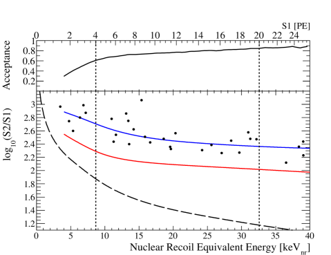
Figure 16: Cut acceptance (top, not including 50% acceptance from $\mathrm{S2/S1}$ discrimination) and discrimination parameter $\log_{10}(\mathrm{S2/S1})$ (bottom) as functions of nuclear recoil energy for events observed in the 40 kg fiducial volume during 11.17 live days of the first XENON100 data release blmbDAprile:2010um . Coloured lines correspond to the median $\log_{10}(\mathrm{S2/S1})$ values of the electronic (blue) and nuclear (red) recoil bands. The dark matter search energy window from 8.7-32.6 keV_nr (vertical, dashed) and the S2 software threshold of 300 PE (long dashed) are also shown. No nuclear recoil events are observed. Figure taken from  blmbDAprile:2010um .

0.58 Short review of the basic idea of the DAMA experiment blmbDDAMA

The basic idea of the DAMA experiment blmbDDAMA is to measure the annual modulation of the rate of events in a large NaI/Tl scintillator. It is expected that the rate should modulate due to the motion of Earth through the cloud of the dark matter particles. Sun itself moves through this cloud as it travels around the center of our galaxy. When Earth and Sun move in the same direction relative to the center of our galaxy, the flux of incoming dark matter particles is increased and therefore also the rate of events measured in the DAMA experiment should correspondingly increase. The expression for the rate is

$$R_{A}=\,N_{A}\,\frac{\rho_{0}}{m_{c_{5}}}\;\sigma(A)\,v_{S}\,\varepsilon_{v_{dmS}}\,\varepsilon_{\rho}\,\left(1+\frac{\varepsilon_{v_{dmES}}}{\varepsilon_{v_{dmS}}}\,\frac{v_{ES}}{v_{S}}\,\cos\theta\,\sin\omega t\right)\,,$$ (443)

where $\theta=60^{o}$ is the angle between the plane of rotation of Earth around Sun and the plane of rotation of Sun around the center of our galaxy. $R_{A}$ is the number of events per unit time and unit active mass of the detector, $\rho_{0}$ is the local mass density of the dark matter which is unknown ( say within the factor of $10$) with respect to the average density (see also the ref. blmbDgn ) and which we take into account with the factor $\varepsilon_{\rho}$, measuring this indeterminacy of the local density of dark matter. In the XENON100 experiment the detector is pure Xe, in the DAMA experiment it is NaI(Tl), in the CDMS experiment it is Ge. In all experiments cuts are applied on data to exclude fake events. The term effective exposure stands for the exposure that takes into account the subsequently reduced acceptance of the experiment with respect to a signal. The probability for a detector to register an event as a dark matter collision is influenced also by the energy threshold of the detector since the detector is blind below the energy threshold. In this analysis we take into account this effect by using a factor $\varepsilon_{cut}$. So if the rate of events taking place in the detector material is $R_{A}$ and the effective exposure is $ex_{{\rm eff}}$, then the average value of events the detector should recognize as the dark matter events is equal to $R_{A}\,ex_{{\rm eff}}\varepsilon_{cut}$. $N_{A}$ is the number of scatterers per unit mass that have atomic mass $A$. In the DAMA experiment it is I ($A_{I}=127$), which for heavy enough dark matter clusters (in the case of the fifth family members of the mass of a few hundred TeV this is the case) contribute the most ($A_{Na}=23$ is in this case negligible). In this case $N_{I}=4.0\times 10^{24}\;\textrm{kg}^{-1}$. In the XENON100 experiment with xenon ($A_{Xe}=131$) $N_{Xe}=4.6\times 10^{24}\;\textrm{kg}^{-1}$. $\sigma(A)$ is the low energy cross section for the collision of the dark matter constituent and the nuclei of the detector. We must point out that this cross section should scale as $\sigma(A)\propto A^{4}$ since for the case when dark matter constituents are for orders of magnitude more massive than the nuclei the scattering is coherent which brings a factor $A^{2}$ while another factor $A^{2}$ comes from the phase space. $v_{S}$ is the velocity of the Sun around the center of our galaxy, which is in the region $100\;{\rm km/s}<v_{S}<270\;{\rm km/s}$. $\varepsilon_{v_{dmS}}$ is an indeterminacy factor that tells how much the flux of dark matter particles onto a detector differs from the flux in the case in which the Sun is moving through the cloud of dark matter particles that are at rest relative to the center of galaxy. In such (rather artificial) case the intrinsic motion of dark matter particles does not increase the flux. This factor depends only on the motion of the dark matter constituents and Sun. $m_{c_{5}}$ is the mass of a dark matter particle. The ratio $\varepsilon_{v_{dmES}}/\varepsilon_{v_{dmS}}$ describes the indeterminacy of the amplitude of the annual modulation of the rate. It depends only on the motion of Sun, Earth and the dark matter. $v_{ES}$ is the velocity of Earth relative to Sun. $\omega$ fixes the period to one year. A detailed description of the analysis is presented in the already mentioned reference blmbDgn . The amplitude of the annual modulation and the average rate are connected in the following way

$$\frac{\Delta R_{A}}{\bar{R}_{A}}=\frac{\varepsilon_{v_{dmES}}}{\varepsilon_{v_{dmS}}}\,\frac{v_{ES}}{v_{S}}\,\cos\theta.$$ (444)

0.59 What should the XENON100 experiment observe if DAMA and XENON100 measure the fifth family neutrons with the mass of several hundred TeV/$c^{2}\,$?

In the following we calculate the number of events the XENON100 experiment should have measured in the first data taking if we assume the events that the DAMA experiment measures in the observed annual modulation are the fifth family neutrons predicted by the spin-charge-family-theory. Similar to the CDMS experiment, the XENON100 experiment has so far measured no events which these two experiments would recognize as dark matter events.

From Eq. (443) and the properties of $\sigma(A)$ we see that $R_{A}\propto N_{A}A^{4}$. The number of events CDMS should have measured is given according to the following formula, where $e_{{\rm eff}\,Xe}=172\;\textrm{kg}\cdot\textrm{day}$ is the effective exposure

$$N = e_{{\rm eff}\,Xe}\;\bar{R}_{Xe}\;\varepsilon_{cut\;Xe}$$ (445)

$$= e_{{\rm eff}\,Xe}\;\varepsilon_{cut\;DAMA}\;\Delta R_{I}\frac{\varepsilon_{v_{dmS}}}{\varepsilon_{v_{dmES}}}\frac{v_{S}}{v_{ES}\cos\theta}\frac{N_{Xe}}{N_{I}}\left(\frac{A_{Xe}}{A_{I}}\right)^{4}\frac{\varepsilon_{cut\;Xe}}{\varepsilon_{cut\;DAMA}}.$$

The experimental value of the measured amplitude of the annual modulation of the DAMA experiment blmbDDAMA is $\Delta R_{I}\;\varepsilon_{cut\;DAMA}=0.052\;\textrm{event}\;\textrm{day}^{-1}\textrm{kg}^{-1}$. For the value $v_{S}=220\;\textrm{km/s}$ we obtain

$$N = 172\cdot 0.052\frac{\varepsilon_{v_{dmS}}}{\varepsilon_{v_{dmES}}}\;14.7\;\frac{4.6}{4.0}\;\left(\frac{131}{127}\right)^{4}\;\frac{\varepsilon_{cut\;Xe}}{\varepsilon_{cut\;DAMA}}$$ (446)

$$= 170\;\frac{\varepsilon_{v_{dmS}}}{\varepsilon_{v_{dmES}}}\;\frac{\varepsilon_{cut\;Xe}}{\varepsilon_{cut\;DAMA}}\,.$$

Let us assume the velocity rangeof Sun within the interval $100{\rm km}/s<v_{S}<270{\rm}km/s$. Then for the Sun’s velocities $v_{S}=(100,\;170,\;220,\;270){\rm km/s}$ we correspondingly obtain the number of events that the XENON100 experiment should measure

$$v_{S} = (100,\;170,\;220,\;270){\rm km/s},$$

$$N = (77,\;\;132,\;170,\;209)\frac{\varepsilon_{v_{dmS}}}{\varepsilon_{v_{dmES}}}\;\frac{\varepsilon_{cut\;Xe}}{\varepsilon_{cut\;DAMA}}\,.$$ (447)

Comparison among different experiments weakens the dependence on most of the uncertainties. What stays is the ratio of the uncertainties about the cuts and the uncertainties in the relative velocities which concern the dark matter properties. The ratio on the uncertainties about the cuts is determined mainly on the threshold of the detectors and it is not expected to be an order of magnitude away from 1. From extreme case models about possible ways of motion of the dark matter constituents in our galaxy, which we performed, we expect the ratio $\frac{\varepsilon_{v_{dmS}}}{\varepsilon_{v_{dmES}}}$, determined by the dynamics of the dark matter constituents in the galaxy, to be from 1/3 to 3. We note that this XENON100 data was taken in November, when signals with strong annual modulation are expected to be rather weak.

Assuming simple Poisson statistics one can quote the probabilities that the XENON100 experiment observes zero events when the average expected number of events is $(3,5,10,100)$

$$(3,\quad\;5,\quad\quad 10,\quad\quad\,100)\;\;\quad{\rm expected\,\,\,events}$$ (448)

$$(5,\quad 0.7,\quad 4\times 10^{-3},10^{-42})\;\%\;{\rm probability\;to\;observe\;zero\,\,\,events}.$$

0.60 Conclusion

A new data release from XENON100 is expected very soon, with an exposure more than an order of magnitude above the published data. This will help to constrain the nature of dark matter also in the scenario of the spin-charge-family-theory that is considered here.

Masses and Mixing Matrices of Families of Quarks and Leptons Within the Approach of
N.S. Mankoč Borštnik Unifying Spins and Charges and predicting families A. Hernández-Galeana¹ and N.S. Mankoč Borštnik²

0.61 Introduction

The approach unifying spin and charges and predicting families (hereafter named the spin-charge-family-theory ansnmbnorma ; ansnmbpikanorma ; ansnmbNF ), proposed by N.S. Mankoč Borštnik, seems promising to show the right way beyond the standard model of fermions and bosons. The reader is kindly asked to learn more about this theory in the ref. ansnmbNF in this proceedings (and in the references therein). Following analyses of the ref. ansnmbNF , we shall here repeat only those parts, which are necessary for the explanation to what conclusions one loop corrections beyond the tree level might lead.

The spin-charge-family-theory predicts eight massless families of quarks and leptons before the two successive breaks – first from $SU(2)_{I}\times SU(2)_{II}\times U(1)_{II}\times SU(3)$ to $SU(2)_{I}\times U(1)_{I}\times SU(3)$ and then from $SU(2)_{I}\times U(1)_{I}\times SU(3)$ to $U(1)\times SU(3)$. Mass matrices originate in a simple starting action: They are determined by the nonzero vacuum expectation values of the scalar (with respect to $SO(1,3)$) fields, to which vielbeins and the two kinds of spin connection fields contribute. Each of the two breaks is triggered by different (orthogonal) superposition of scalar fields. The mass matrices for eight families appear to be four times four by diagonal matrices, with no mixing matrix elements among the upper four and the lower four families. There are, correspondingly, two (with respect to the life of our Universe) stable families: the fifth and the observed first family. The fifth family members are candidates to form the dark matter, the fourth family waits to be observed.

After the first break (from $SU(2)_{II}\times SU(2)_{I}\times U(1)_{II}\times SU(3)$ to $SU(2)_{I}\times U(1)_{I}\times SU(3)$), which occurs, below $\approx 10^{13}$ GeV, the upper four families become massive. In the second break, which is the standard model-like electroweak break, also the lower four families became massive.

Rough estimations made so far ansnmbpikanorma ; ansnmbgmdn ; ansnmbgn on the tree level, which took into account besides the elementary particle data also the cosmological data, show that the stable of the upper four families might have masses ansnmbgn of the order of $100$ TeV/$c^{2}$. The contribution ansnmbMN discusses also the possibility that the masses are much smaller, of around a few TeV/$c^{2}$. For the lower four families ansnmbpikanorma ; ansnmbgmdn we were not really able to predict the masses of the fourth family members, we only estimated for chosen masses of the fourth family members their mixing matrices.

In this contribution we are studying, following suggestions from the ref. ansnmbNF , properties of the mass matrices of twice four families, taking into account the one loop corrections to the tree level estimations. We namely hope to see already within the one and may be two loops corrections the explanation for the differences in masses and mixing matrices between quarks and leptons, as well as within quarks and within leptons.

To the loop corrections the gauge boson fields and the scalar field contribute, as explained in the ref. ansnmbNF .

Let us write the effective action (it is from the ref. ansnmbNF as Eq. (5)) for eight families of quarks and leptons ($\psi$), left and right handed. The action is formally rewritten in a way to manifest the standard model properties

$${\mathcal{L}}_{f} = \bar{\psi}\gamma^{m}(p_{m}-\sum_{A,i}\;g^{A}\tau^{Ai}A^{Ai}_{m})\psi+$$ (449)

$$\{\sum_{s=7,8}\;\bar{\psi}\gamma^{s}p_{0s}\;\psi\}+$$

$${\rm the\;rest},$$

where $m=0,1,2,3$ with

$$\tau^{Ai}=\sum_{a,b}\;c^{Ai}{}_{ab}\;S^{ab},$$

$$\{\tau^{Ai},\tau^{Bj}\}_{-}=i\delta^{AB}f^{Aijk}\tau^{Ak}.$$ (450)

The second row of Eq. (449) defines the mass matrices. We shall call it ${\mathcal{L}}_{Y}$. We namely have (Eq. (26)in the ref. ansnmbNF )

$${\mathcal{L}}_{Y} = \psi^{\dagger}\,\gamma^{0}\,(\stackrel{{\scriptstyle 78}}{{(+)}}p_{0+}+\stackrel{{\scriptstyle 78}}{{(-)}}p_{0-}\,\psi,$$

$$p_{0\pm} = p_{07}\mp ip_{08},\quad p_{0s}=p_{s}-\frac{1}{2}\,\tilde{S}^{ab}\,\tilde{\omega}_{abs}-\frac{1}{2}\,S^{ab}\,\omega_{abs},$$ (451)

with $s=7,8,$ and $\stackrel{{\scriptstyle 78}}{{(\pm)}}=\frac{1}{2}\,(\gamma^{7}\pm\gamma^{8})$. $\stackrel{{\scriptstyle 78}}{{(-)}}$ transforms, for example, a righ handed $u_{R}$-quark of a particular colour and spin to the corresponding left handed $u_{L}$-quark of the same spin and colour.

We see that to the mass terms both, $\tilde{S}^{ab}\,\tilde{\omega}_{abs}$ (transforming one family into another) as well as $S^{ab}\,\omega_{abs}$ might contribute (a superposition which ”sees” the electromagnetic charge $Q$ and the quantum number $Q^{\prime}$) whenever the spin connection scalar fields $\omega_{abs}$ and $\tilde{\omega}_{abs}$, each in a superposition determined by a particular break, gain nonzero vacuum expectation values.

To the first break (when one of the two $SU(2)$ together with $U(1)$ breaks, namely $SU(2)_{II}\times U(1)_{II}$ breaks into $U(1)_{I}$) the scalar fields (with respect to $SO(1,3)$) originating in vielbeins and particular superposition of spin connection fields of $\tilde{S}^{ab}$ contribute.

From the ref. ansnmbNF we read in Table 14 a general shape of mass matrices after the first break, when the upper four families gain masses, while the lower four families are still massless. We present this table, Table 15, also here. To learn the meaning of the notation $\tilde{a}^{\tilde{A}i}_{\pm}$ the reader should look at Section V. of the ref. ansnmbNF . For discussions here only the symmetry of mass matrices is important. $(\pm)$ distinguishes between the values of the $u$-quarks and $d$-quarks and between the values of $\nu$ and $e$.

	$I$	$II$	$III$	$IV$	$V$	$VI$	$VII$	$VIII$
$I\;\;\;$	$\;0\;$	$\;0\;$	$\;0\;$	$\;0\;$	$0$	$0$	$0$	$0$
$II\;\;$	$0$	$0$	$0$	$0$	$0$	$0$	$0$	$0$
$III\;$	$0$	$0$	$0$	$0$	$0$	$0$	$0$	$0$
$IV\;\,$	$0$	$0$	$0$	$0$	$0$	$0$	$0$	$0$
$V\;\;$	$0$	$0$	$0$	$0$	$\frac{1}{2}\,(\tilde{a}^{23}_{\pm}+\tilde{a}^{\tilde{N}^{3}_{R}}_{\pm})$	$-\tilde{a}^{2-}_{\pm}$	$-\tilde{a}^{\tilde{N}_{R}^{+}}_{\pm}$	$0$
$VI\;\,$	$0$	$0$	$0$	$0$	$-\tilde{a}^{2+}_{\pm}$	$\frac{1}{2}(-\tilde{a}^{23}_{\pm}+\tilde{a}^{\tilde{N}^{3}_{R}}_{\pm})$	$0$	$-\tilde{a}^{\tilde{N}_{R}^{+}}_{\pm}$
$VII\;$	$0$	$0$	$0$	$0$	$-\tilde{a}^{\tilde{N}_{R}^{-}}_{\pm}$	$0$	$\frac{1}{2}\,(\tilde{a}^{23}_{\pm}-\tilde{a}^{\tilde{N}^{3}_{R}}_{\pm})$	$-\tilde{a}^{2-}_{\pm}$
$VIII$	$0$	$0$	$0$	$0$	$0$	$-\tilde{a}^{\tilde{N}_{R}^{-}}_{\pm}$	$-\tilde{a}^{2+}_{\pm}$	$-\frac{1}{2}\,(\tilde{a}^{23}_{\pm}+\tilde{a}^{\tilde{N}^{3}_{R}}_{\pm})$

Table 15: The mass matrix for the eight families of quarks and leptons after the break of $SO(1,3)\times SU(2)_{I}\times SU(2)_{II}\times U(1)_{II}\times SU(3)$ to $SO(1,3)\times SU(2)_{I}\times U(1)_{I}\times SU(3)$. The contribution comes from a particular superposition of spin connection fields, the gauge fields of $\tilde{S}^{ab}$. $(\mp)$ distinguishes $u_{i}$ from $d_{i}$ and $\nu_{i}$ from $e_{i}$.

To the second break (when the remaining $SU(2)$ contributes, namely $SU(2)_{I}\times U(1)_{I}$ breaks into $U(1)$) besides the scalar fields originating in vielbeins and in orthogonal (to the first) superposition of spin connection fields of $\tilde{S}^{ab}$, also the scalar fields originating in spin connections of $S^{ab}$ contribute. This is explained in the ref. ansnmbNF .

Table 16 represents the mass matrices for the lower four families on the tree level. Only the contribution of the scalar fields which originate in the gauge fields of $\tilde{S}^{ab}$ are included. The contribution from the terms like $Q^{\prime}\,A^{Q^{\prime}}_{s}$, which are diagonal and equal for all the families, but distinguish among the members of one family are not present. The notation $\tilde{a}^{\tilde{A}i}_{\pm}=$ $-\tilde{g}^{\tilde{A}i}\,\tilde{A}^{\tilde{A}i}_{\pm}$ is used.

	$I$	$II$	$III$	$IV$
$I\;\;$	$\frac{1}{2}\,(\tilde{a}^{13}_{\pm}+\tilde{a}^{\tilde{N}^{3}_{L}}_{\pm})$	$\tilde{a}^{1+}_{\pm}$	$\tilde{a}^{\tilde{N}_{L}^{+}}_{\pm}$	$0$
$II\;$	$\tilde{a}^{1-}_{\pm}$	$\frac{1}{2}(-\tilde{a}^{13}_{\pm}+\tilde{a}^{\tilde{N}^{3}_{L}}_{\pm})$	$0$	$\tilde{a}^{\tilde{N}_{L}^{+}}_{\pm}$
$III$	$\tilde{a}^{\tilde{N}_{L}^{-}}_{\pm}$	$0$	$\frac{1}{2}\,(\tilde{a}^{13}_{\pm}-\tilde{a}^{\tilde{N}^{3}_{L}}_{\pm})$	$\tilde{a}^{1+}_{\pm}$
$IV$	$0$	$\tilde{a}^{\tilde{N}_{L}^{-}}_{\pm}$	$\tilde{a}^{1-}_{\pm}$	$-\frac{1}{2}\,(\tilde{a}^{13}_{\pm}+\tilde{a}^{\tilde{N}^{3}_{L}}_{\pm})$

Table 16: The mass matrix for the lower four families of quarks and leptons after the electroweak break. Only the contributions coming from the spin connection fields, originating in $\tilde{S}^{ab}$ are presented. $(\mp)$ distinguishes between the values of the $u$-quarks and $d$-quarks and between the values of $\nu$ and $e$. The terms coming from spin connection fields originating in $S^{ss^{\prime}}\,$ are not presented here. They are the same for all the families, but distinguish among the family members.

We shall study in this contribution the properties of only the lowest two families of each of the two groups of families, neglecting the nonzero mass matrix elements between the lower and the upper two families, which on the tree level looks in the spin-charge-family-theory rather small, in particular for the upper four families. The measured values of the mixing matrices for the observed families supports such an assumption for quarks, at least for these first studies, but not for leptons. Of course, going beyond the tree level can drastically change the values of matrix elements, what obviously must happen at least for leptons of the lower four families.

0.62 Mass matrices beyond the tree level

It seems meaningful ansnmbNF , that is in accordance with the experimental data, to assume that to the upper four families only $\tilde{\omega}_{abs}$ contribute on the tree level, while for the lower four families also the fields $\omega_{stt^{\prime}}$ contribute a diagonal terms, the same for all the families of a particular member, but different for different family members.

We shall study in this contribution, as we already say, only mass matrices of the lowest two families, that is only two times two matrices, for either the upper or the lower four families, neglecting the coupling to the rest of the two families. That is we shall put the matrix elements $\tilde{a}^{\tilde{N}^{3,\pm}_{L,R}}_{\pm}=0$, in both tables, Table 15 and Table 16, since the spin-charge-family-theory suggets that these are much smaller than the rest of matrix elements.

Regarding the upper group of families the $2\times 2$ mass matrices look accordingly like

$$M_{\pm}^{\scriptstyle{V,VI}}=\begin{pmatrix}a_{1}&b\\ b&a_{2}\end{pmatrix}^{\scriptstyle{V,VI}}_{\pm}\;,$$ (452)

the same for $u_{i}$ and $\nu_{i}$ $(-)$ and for $d_{i}$ and $e_{i}$ $(+)$.

For the lowest two families to the mass matrix $M_{\pm}^{\scriptstyle{I,II}}$ a different diagonal term $a^{\alpha}\,I_{2\times 2}$ should be added for each of the family member $\alpha=u,d,\nu,e$, where $I$ is the identity matrix.

$$M^{\alpha,\scriptstyle{I,II}}=a^{\alpha}\,I_{2\times 2}+\begin{pmatrix}a_{1}&b\\ b&a_{2},\end{pmatrix}^{\scriptstyle{I,II}}_{\pm}\;.$$ (453)

Let us, before going to the loop corrections, diagonalize these tree level matrices. If we write any of the mass matrices (for any member of either the upper two or the lower two families)

$${\cal M}_{o}=\begin{pmatrix}a_{1}&b\\ b&a_{2}\end{pmatrix}$$ (454)

and any of the two correcponding (left and right handed) vectors as

$$\psi_{L,R}^{o}=\begin{pmatrix}\psi_{1}^{o}\\ \psi_{2}^{o}\end{pmatrix}_{L,R}\;,$$ (455)

then a generic mass term from Eq.(0.61) and presented in tables 15,16, only $2\times 2$ matrices, can be diagonalized with the orthogonal matrix

$$V=\begin{pmatrix}\cos\theta&\sin\theta\\ -\sin\theta&\cos\theta\end{pmatrix}\quad,\quad\cos\theta=\sqrt{\frac{a_{2}-m_{1}}{m_{2}-m_{1}}}\;\;,\;\;\sin\theta=\sqrt{\frac{a_{1}-m_{1}}{m_{2}-m_{1}}}$$ (456)

with $m_{1,2}=\frac{1}{2}\,[(a_{1}+a_{2})\mp\,\sqrt{(a_{1}+a_{2})^{2}-4\,(a_{1}a_{2}-b^{2})}]$. We have

$$\psi_{L,R}^{o}=V\>\psi_{L,R}\quad;\quad V^{T}{\cal M}_{o}\>V=M_{D}=Diag(m_{1},m_{2})$$ (457)

with $m_{1}$ and $m_{2}$ the mass eigenvalues of ${\cal M}_{o}$, and

$$\bar{\psi_{L}^{o}}\>{\cal M}_{o}\>\psi_{R}^{o}=\bar{\psi_{L}}\>M_{D}\>\psi_{R}$$ (458)

.

0.62.1 Gauge bosons $A_{m}^{Y^{\prime}}$ contribution to one loop corrections

What follows can be found in Subsection IV.B. of the ref. ansnmbNF . Let us first treat the upper two (out of four) families. From the expressions which will be obtained for the upper two (out of four) families it is not difficult to obtain the corresponding expressions for the lowest two families.

According to the ref. ansnmbNF $\psi_{R}^{o}$ transforms as $(2,\tau^{4})$, $\tau^{4}=\frac{1}{6}$ ($-\frac{1}{2}$) for quarks (leptons), under $SU(2)_{II}\times U(1)_{II}$, while $\psi_{L}^{o}$ transforms as $(1,\tau^{4})$ under $SU(2)_{II}\times U(1)_{II}$. Therefore the covariant momenta contributing to the mass matrices are

$$p_{om}\>\psi_{R}^{o}=\{p_{m}- \bigl{[} g_{Y}\>Y\>A_{m}^{Y}+g_{2}\>\cos\theta_{2}\>Y^{\prime}\>A_{m}^{Y^{\prime}}+$$ (459)

$$\frac{1}{\sqrt{2}}\left(\tau^{2+}A_{m}^{2+}+\tau^{2-}A_{m}^{2-}\right)\bigr{]}\,\}\>\psi_{R}^{o}\,,$$

and

$$p_{om}\>\psi_{L}^{o} = \{p_{m}-g_{4}\tau^{4}\>A_{m}^{\tau^{4}}\}\,\>\psi_{L}^{o}=$$ (460)

$$= \{p_{m}-\left(g_{4}\>\tau^{4}\cos\theta_{2}\>A_{m}^{Y}-g_{4}\>\tau^{4}\sin\theta_{2}\>A_{m}^{Y^{\prime}}\right)\,\}\>\psi_{L}^{o}\,.$$

From these expressions for the covariant derivatives the gauge couplings to $A_{m}^{Y^{\prime}}$ follow

$$g_{u_{iL}}^{\prime}\bar{u}_{iL}\gamma^{m}A_{m}^{Y^{\prime}}u_{iL}+g_{u_{iR}}^{\prime}\bar{u}_{iR}\gamma^{m}A_{m}^{Y^{\prime}}u_{iR}$$ (461)

$$g_{\nu_{iL}}^{\prime}\bar{\nu}_{iL}\gamma^{m}A_{m}^{Y^{\prime}}\nu_{iL}+g_{\nu_{iR}}^{\prime}\bar{\nu}_{iR}\gamma^{m}A_{m}^{Y^{\prime}}\nu_{iR}$$ (462)

,

with $i=V,VI$, and where

$$g_{u_{iL}}^{\prime}=-\frac{1}{6}g_{4}\sin\theta_{2}\quad;\quad g_{u_{iR}}^{\prime}=g_{2}\cos\theta_{2}\>\frac{1}{2}(1-\frac{1}{3}\tan^{2}\theta_{2})\;,$$ (463)

$$g_{\nu_{iL}}^{\prime}=\frac{1}{2}g_{4}\sin\theta_{2}\quad;\quad g_{\nu_{iR}}^{\prime}=g_{2}\cos\theta_{2}\>\frac{1}{2}(1+\tan^{2}\theta_{2})\;,$$ (464)

with $\sin\theta_{2}$ and $\cos\theta_{2}$ defined by the relationship

$$g^{Y}=\frac{g^{2}\>g^{4}}{\sqrt{(g^{2})^{2}+(g^{4})^{2}}}=g^{2}\>\sin\theta_{2}=g^{4}\>\cos\theta_{2}\;,$$ (465)

$g^{2},\>g^{4}\>g^{Y}$ being the couplings of $SU(2)_{II}$, $U(1)_{II}$ and $U(1)_{I}$, respectively.

Figure 17: One loop contribution from $A_{m}^{Y^{\prime}}$ gauge boson.

The tree level mass terms and gauge couplings may be used to draw the one loop diagrams of Fig. 17. We write the internal fermion lines of these diagrams in terms of the mass eigenvalues and eigenfields of ${\cal M}_{o}$. So, the one loop contribution in the interaction basis reads

$$\bar{\psi_{L}^{o}}\>{\cal M}_{1}^{\prime}\>\psi_{R}^{o}=\bar{\psi_{L}}\>V^{T}\>{\cal M}_{1}^{\prime}\>V\>\psi_{R}\qquad;\qquad{\cal M}_{1}^{\prime}=\begin{pmatrix}w_{11}&w_{12}\\ w_{21}&w_{22}\end{pmatrix}\>,$$ (466)

where

$$w_{11}=\cos^{2}\theta\>m_{1}\>G_{1}+\sin^{2}\theta\>m_{2}\>G_{2}\;,$$ (467)

$$w_{22}=\sin^{2}\theta\>m_{1}\>G_{1}+\cos^{2}\theta\>m_{2}\>G_{2}\;,$$ (468)

$$w_{21}=w_{12}=\cos\theta\>\sin\theta\>(-m_{1}\>G_{1}+m_{2}\>G_{2})\;,$$ (469)

$$G_{i}\equiv G(M,m_{i})=\frac{g_{L}^{\prime}\>g_{R}^{\prime}}{16\>\pi^{2}}\>\frac{M^{2}}{M^{2}-m_{i}^{2}}\ln{\frac{M^{2}}{m_{i}^{2}}}\quad,\quad M^{2}=M_{A^{Y^{\prime}}}^{2}\;,$$ (470)

where the corresponding couplings $(g_{L}^{\prime}\>g_{R}^{\prime})_{ui}$ and $(g_{L}^{\prime}\>g_{R}^{\prime})_{\nu i}$ read from from Eqs.(463,464).

Explicit computation yields

$${V}^{T}\>{\cal M}_{1}^{\prime}\>V=\begin{pmatrix}m_{1}\>G_{1}&0\\ 0&m_{2}\>G_{2}\end{pmatrix}$$ (471)

Hence the one loop contributions from $A^{Y^{\prime}}$ give corrections to the tree level mass eigenvalues, but does not correct mixing.

0.62.2 Scalar fields contribution to one loop corrections

Following an analogous procedure as in the previous subsection we calculate in what follows the contribution from the scalar fields, the scalar fields of $\tilde{S}^{ab}$, to loop corrections. Couplings of heavy families $V$ and $VI$ to the scalar tilde fields $\tilde{A}^{2i}_{\pm}$ are

$$\frac{\tilde{g}_{2}}{2}\>\left[\left(\overline{\psi_{2}^{o}}_{L,R}\>{\psi_{1}^{o}}_{R,L}+\overline{\psi_{1}^{o}}_{L,R}\>{\psi_{2}^{o}}_{R,L}\right)\>\tilde{A}^{21}_{\pm}\right.\\ +\left(i\>\overline{\psi_{2}^{o}}_{L,R}\>{\psi_{1}^{o}}_{R,L}-i\>\overline{\psi_{1}^{o}}_{L,R}\>{\psi_{2}^{o}}_{R,L}\right)\>\tilde{A}^{22}_{\pm}\\ +\left.\left(\overline{\psi_{1}^{o}}_{L,R}\>{\psi_{1}^{o}}_{R,L}-\overline{\psi_{2}^{o}}_{L,R}\>{\psi_{2}^{o}}_{R,L}\right)\>\tilde{A}^{23}_{\pm}\right]$$ (472)

Using these scalar couplings and the tree level mass matrices for the upper two family members $\psi_{iR,L},i=V,VI$, first for $u_{iL,R}$ quarks and neutrinos $\nu_{iL,R}$, we can draw the one loop diagrams of Figs. 18 and 19.

Figure 18: Loop contributions from $\tilde{A}_{-}^{2\pm}$.

Figure 19: Loop contributions from $\tilde{A}_{-}^{23}$.

It follows then

$$\bar{\psi_{L}^{o}}\>\tilde{\cal M}_{1}\>\psi_{R}^{o}=\bar{\psi_{L}}\>V^{T}\>\tilde{\cal M}_{1}\>V\>\psi_{R}\qquad;\qquad\tilde{\cal M}_{1}=\begin{pmatrix}\Omega_{11}&\Omega_{12}\\ \Omega_{21}&\Omega_{22}\end{pmatrix}\>,$$ (473)

with

$$\Omega_{11}=2\left(\sin^{2}\theta\>\Sigma_{1}^{1}+\cos^{2}\theta\>\Sigma_{2}^{1}\right)+\cos^{2}\theta\>\Sigma_{1}^{3}+\sin^{2}\theta\>\Sigma_{2}^{3}$$ (474)

$$\Omega_{22}=2\left(\cos^{2}\theta\>\Sigma_{1}^{1}+\sin^{2}\theta\>\Sigma_{2}^{1}\right)+\sin^{2}\theta\>\Sigma_{1}^{3}+\cos^{2}\theta\>\Sigma_{2}^{3}$$ (475)

$$\Omega_{21}=\Omega_{12}=\cos\theta\>\sin\theta\>(\Sigma_{1}^{3}-\Sigma_{2}^{3})$$ (476)

$$\Sigma_{i}^{j}\equiv m_{i}\>{\cal G}(M_{j},m_{i})\;,\;{\cal G}(M_{j},m_{i})=\frac{\tilde{g}_{2}^{2}}{4}\>\frac{1}{16\>\pi^{2}}\>\frac{M_{j}^{2}}{M_{j}^{2}-m_{i}^{2}}\ln{\frac{M_{j}^{2}}{m_{i}^{2}}}$$ (477)

$$M_{1}^{2}=M_{\tilde{A}^{21}}^{2}=M_{\tilde{A}^{22}}^{2}\qquad,\qquad M_{3}^{2}=M_{\tilde{A}^{23}}^{2}$$ (478)

Let us remind here that the scalar fields $\tilde{A}^{23}$ and $\tilde{A}^{4}$ mix in the breaking $SU(2)_{II}\times U(1)_{II}$ into $U(1)_{I}$ (Eq.(19) in the ref.ansnmbNF ), so that it is consistent to consider $M_{1}\neq M_{3}$ in Eq.(478).

From explicit computation one gets

$$\Gamma={V}^{T}\>\tilde{\cal M}_{1}\>V=\begin{pmatrix}\Gamma_{11}&\Gamma_{12}\\ \Gamma_{21}&\Gamma_{22}\end{pmatrix}$$ (479)

where

$$\Gamma_{11}=2\>\Sigma_{2}^{1}+\Sigma_{1}^{3}-4\cos^{2}\theta\>\sin^{2}\theta\left(\Sigma_{1}^{3}-\Sigma_{1}^{1}+\Sigma_{2}^{1}-\Sigma_{2}^{3}\right)$$ (480)

$$\Gamma_{22}=2\>\Sigma_{1}^{1}+\Sigma_{2}^{3}+4\cos^{2}\theta\>\sin^{2}\theta\left(\Sigma_{1}^{3}-\Sigma_{1}^{1}+\Sigma_{2}^{1}-\Sigma_{2}^{3}\right)$$ (481)

$$\Gamma_{21}=\Gamma_{12}=2\>\cos\theta\>\sin\theta\>(\cos^{2}\theta-\sin^{2}\theta)\left(\Sigma_{1}^{3}-\Sigma_{1}^{1}+\Sigma_{2}^{1}-\Sigma_{2}^{3}\right)\;,$$ (482)

where we may write

$$\Sigma_{1}^{3}-\Sigma_{1}^{1}+\Sigma_{2}^{1}-\Sigma_{2}^{3}=\frac{\tilde{g}_{2}^{2}}{64\>\pi^{2}}\>F(M_{1},M_{3},m_{1},m_{2})$$ (483)

with

$$F(M_{1},M_{3},m_{1},m_{2})=\left\{m_{1}\left[\frac{M_{3}^{2}}{M_{3}^{2}-m_{1}^{2}}\ln{\frac{M_{3}^{2}}{m_{1}^{2}}}-\frac{M_{1}^{2}}{M_{1}^{2}-m_{1}^{2}}\ln{\frac{M_{1}^{2}}{m_{1}^{2}}}\right]\right.\\ \\ \left.-m_{2}\left[\frac{M_{3}^{2}}{M_{3}^{2}-m_{2}^{2}}\ln{\frac{M_{3}^{2}}{m_{2}^{2}}}-\frac{M_{1}^{2}}{M_{1}^{2}-m_{2}^{2}}\ln{\frac{M_{1}^{2}}{m_{2}^{2}}}\right]\right\}$$ (484)

Finally, taking into account the tree level contribution, we obtain up to one loop corrections the mass matrix

$$\bar{\psi}_{L}\>\left[V^{T}\>{\cal M}_{1}^{\prime}\>V+V^{T}\>\tilde{\cal M}_{1}\>V+Diag(m_{1},m_{2})\right]\psi_{R}\equiv\bar{\psi}_{L}\>{\cal M}\>\psi_{R}$$ (485)

$${\cal M}=\begin{pmatrix}M_{11}&M_{12}\\ M_{21}&M_{22}\end{pmatrix}\>,$$ (486)

with the mass matrix elements

$$M_{11}=m_{1}+m_{1}\>G_{1}+\Gamma_{11}\quad,\quad M_{22}=m_{2}+m_{2}\>G_{2}+\Gamma_{22}$$ (487)

$$M_{21}=M_{12}=\Gamma_{12}$$ (488)

Diagonalizing the mass matrix ${\cal M}$, Eq.(486), the physical masses for fermions within one loop correction follow.

Notice that in the limit $m_{1},m_{2}\ll M_{1},M_{3}$, which is accomplished for at least the lower 1 and 2 families, we may approach

$$F(M_{1},M_{3},m_{1},m_{2})\approx(m_{2}-m_{1})\>\ln{\frac{M_{1}^{2}}{M_{3}^{2}}}\;,$$ (489)

and

$$\Sigma_{i}^{j}\approx\frac{\tilde{g}_{2}^{2}}{64\>\pi^{2}}\>m_{i}\>\ln{\frac{M_{j}^{2}}{m_{i}^{2}}}\;,$$ (490)

So, the mass terms $M_{ij}$ in this limit may be written explicitly as

$$M_{11}\thickapprox m_{1}+m_{1}\>\frac{g_{L}^{\prime}\>g_{R}^{\prime}}{16\>\pi^{2}}\>\ln{\frac{M^{2}}{m_{1}^{2}}}\\ +\frac{\tilde{g}_{2}^{2}}{64\>\pi^{2}}\>\left[2m_{2}\>\ln{\frac{M_{1}^{2}}{m_{2}^{2}}}+m_{1}\>\ln{\frac{M_{3}^{2}}{m_{1}^{2}}}-4\cos^{2}\theta\sin^{2}\theta\>(m_{2}-m_{1})\>\ln{\frac{M_{1}^{2}}{M_{3}^{2}}}\right]$$ (491)

$$M_{21}=M_{12}\thickapprox\frac{\tilde{g}_{2}^{2}}{32\>\pi^{2}}\>\cos\theta\>\sin\theta\>(\cos^{2}\theta-\sin^{2}\theta)\>(m_{2}-m_{1})\>\ln{\frac{M_{1}^{2}}{M_{3}^{2}}}$$ (492)

$$M_{22}\thickapprox m_{2}+m_{2}\>\frac{g_{L}^{\prime}\>g_{R}^{\prime}}{16\>\pi^{2}}\>\ln{\frac{M^{2}}{m_{2}^{2}}}\\ +\frac{\tilde{g}_{2}^{2}}{64\>\pi^{2}}\>\left[2m_{1}\>\ln{\frac{M_{1}^{2}}{m_{1}^{2}}}+m_{2}\>\ln{\frac{M_{3}^{2}}{m_{2}^{2}}}+4\cos^{2}\theta\>\sin^{2}\theta\>(m_{2}-m_{1})\>\ln{\frac{M_{1}^{2}}{M_{3}^{2}}}\right]$$ (493)

0.63 Discussion and Conclusions

The results reported from the analysis of one loop diagrams coming from $A_{m}^{Y^{\prime}}$ gauge boson and the scalar tilde fields $\tilde{A}^{2i}$ show that loop corrections contribute to both fermion masses and mixing. A detailed quantitative analysis is in progress to find out the spectrum of masses and mixing that we are able to accommodate taking into account tree level and loop corrections. Even without present here some numerical results, it is important to point out that for the upper two families the main differences among family mass matrices, for instance between very heavy U quarks and neutrinos N, come from loop corrections, while for the lower two families the diagonal mass terms, differing for each family member and being the same for all families, play an important role together with the loop contributions to distinguish for example between up quarks and neutrino mass matrices within this spin-charge-family theory.

The expressions for the mass terms $M_{ij}$ as written in Eqs.(491-493) are useful to obtain the quantitative corrections to the the tree level masses and mixing from loop contributions at least for the lower 1 and 2 families.

Can the Stable Fifth Family of the ”Spin-charge-family-theory” Proposed by N.S. Mankoč Borštnik Fulfil the M.Y. Khlopov Requirements and Form the Fifth Antibaryon Clusters with Ordinary He Nucleus? M. Y. Khlopov^1,2,3 and N.S. Mankoč Borštnik⁴

0.64 Introduction

The theory unifying spin and charges and predicting families – the spin-charge-family-theory – proposed by N. S. Mankoč Borštnik mksnmbDnorma ; mksnmbDpikanorma ; mksnmbDNF is very promising in showing the right way beyond the standard model.

• It predicts families and their mass matrices, explaining the origin of the charges and of the gauge fields mksnmbDnorma ; mksnmbDpikanorma ; mksnmbDNF .

• It predicts that there are, before the universe passes through the two $SU(2)\times U(1)$ phase transitions, eight massless families of quarks and leptons mksnmbDNF .

• It predicts after these two phase transitions, in which the symmetry breaks from $SO(1,3)\times SU(2)\times SU(2)\times U(1)\times SU(3)$ first to $SO(1,3)\times SU(2)\times U(1)\times SU(3)$ and then to $SO(1,3)\times U(1)\times SU(3)$, twice decoupled four families. The upper four families gain masses in the first phase transition, while the second four families gain masses at the electroweak break. To these two breaks of symmetries the scalar non Abelian fields, the (superposition of the) gauge fields of the operators generating families, contribute mksnmbDNF .

• The lightest of the upper four families is stable (in comparison with the life of the universe) and is therefore a candidate for constituting the dark matter. Their masses are so far only roughly estimated mksnmbDgn ; mksnmbDMN to be around a few hundred TeV/$c^{2}$.

• The heaviest of the lower four families should be seen at the LHC or at somewhat higher energies mksnmbDpikanorma ; mksnmbDgmdn . The calculations below the tree level are under considerations mksnmbDAN .

There are still many open questions to be solved in this spin-charge-family-theory, which are not directly connected with the question about the dark matter content. Many a problem is shared with many other theories. This discussion concerns mainly the question which one (if any) of the two scenarios for the dark matter constituents has a better chance to be the right one.

Each of these two scenarios lies on the assumptions and rough estimations. We kindly ask the reader to learn more about the spin-charge-family-theory, their assumptions and so far made estimations in the two contributions of Norma in this proceedings mksnmbDNF ; mksnmbDNMA and in the papers cited therein. Here we will present only those estimations that are relevant for this discussion. That is that they help to distinguish between the two proposals for the constituents of the dark matter, if both originating in the stable fifth family members of the spin-charge-family-theory.

The assumptions (many of them supported by rough estimations) and the open questions concerning the Norma’s proposal for the dark matter constituents, which are relevant for this discussion, are presented below. Many an item concerns also the Maxim’s proposal. When commenting the items, which follow, also comments to some of the open problems concerning the Maxim’s proposal are added. Some additional discussions and comments about the open questions concerning the Maxim’s proposal are presented in section 0.65.

1. The masses of the upper four families lie above the lower four families and below the unification scale of the three charges mksnmbDpikanorma ; mksnmbDNF ; mksnmbDgn , say, below $10^{16}$ GeV/$c^{2}$.

2. The masses of each of the member of the upper four families, and consequently also of the fifth family members, are approximately the same at least on the tree level mksnmbDNF .

3. Close below the weak $SU(2)\times U(1)$ phase transition the number density of the fifth family neutrinos (with approximately the same masses as the fifth family electrons and quarks) is pretty much reduced due to a strong neutrino-antineutrino annihilation mksnmbDGN . The contribution of the fifth family neutrinos to the dark matter is then smaller (at least not larger) than the contribution of the fifth family neutrons, provided that the neutrino-antineutrino asymmetry is small enough.

4. In the colour phase transition, which appears at the temperature close below $1$/$k_{b}$ GeV, the coloured fifth family objects either annihilate with the anti-objects or form the colourless neutrons and anti-neutrons and correspondingly decouple from the plasma at the very beginning of the colour phase transition due to very strong binding energies of the fifth family baryons mksnmbDgn ; mksnmbDGNC .

5. Among the open (not yet studied) questions of the spin-charge-family-theory is what is the origin of the matter-antimatter in the universe and how does the fermion-antifermion asymmetry manifest in the case of the stable fifth family.

6. Some additional open question will be discussed in section 0.65.

Comments to the first assumption: This assumption is mild, provided that the universe really passed through two separate phase transitions of the kind as follow: First from $SO(1,3)\times SU(2)\times SU(2)\times U(1)\times SU(3)$ to $SO(1,3)\times SU(2)\times U(1)\times SU(3)$ and then to $SO(1,3)\times U(1)\times SU(3)$.

Comments to the second assumption: Rough estimations show mksnmbDNF that at least on the tree level, but also within one or two loops calculations mksnmbDAN , there is not much possibility for large mass differences among the fifth family members. If the difference ($m_{u_{5}}-m_{d_{5}}$) is not larger than a few hundred GeV/$c^{2}$ in the case of the few hundred TeV/$c^{2}$ quark masses, then the neutron is the stable fifth family member mksnmbDgn ; mksnmbDMN due to repulsive electromagnetic interaction among quarks (and taking into account also the weak interaction). For lighter quark masses smaller differences among the masses of the members are allowed if the fifth family neutron should be the lightest fifth family baryon. For large enough current mass differences, that is for lighter enough fifth family $u_{5}$-quark with respect to $d_{5}$-quark, it might happen that ($\bar{u}_{5}\bar{u}_{5}\bar{u}_{5}$) be the lightest fifth family antibaryon, although it does not look very probable.

Comments to the third assumption: Besides the fifth family colourless clusters of quarks also fifth family neutrinos contribute to the dark matter. If the masses of these neutrinos are a few hundred TeV/$c^{2}$, approximately the same as the masses of the other fifth family members, their contribution to the dark matter would not be in agreement with the measured dark matter density, it would be high to huge. So far done rough estimations (which are still under consideration) show that the number density of the fifth family neutrinos is pretty much reduced due to the neutrino-antineutrino annihilation (the higher is the mass the stronger is annihilation), provided that the fifth family neutrino-antineutrino asymmetry is small enough. The weak annihilation cross section is expected to play much stronger role for neutrinos than for strongly bound quarks in the neutron (due to the huge binding energy of the fifth family quarks), which remains to be proved.

A too large fifth family neutrino-antineutrino asymmetry would lead to contradiction with the experimental data for both proposals for the dark matter constituents, either the Norma’s or the Maxim’s ones.

Comments to the fourth assumption: Norma mksnmbDgn has estimated how do in the colour phase transition behave heavy enough (with the masses of a few hundred TeV/$C^{2}$ or more) coloured fifth family objects, that is single quarks or clusters of quarks. This estimation suggests that the coloured objects either annihilate with the anti-objects or form the colourless neutrons and anti-neutrons and correspondingly decouple from the plasma at the very beginning of the colour phase transition due to very strong binding energies of the fifth family baryons (with respect to the first family baryons). This happens long enough before the first family quarks start to form the baryons, so that there is negligible amount of colourless clusters with the fifth and first family quarks.

If the masses of the fifth family quarks would be of the order of hundreds GeV, for example, or lower, the colourless only fifth family clusters, which would succeed to decouple from plasma, would be very rare. Mostly they would behave similarly as the first family coloured objects. They would either annihilate during the colour phase transition if there would be no quark-antiquark asymmetry or form stable colourless objects with the first family quarks or antiquarks. This estimation needs to be followed by more accurate studies to be proved.

Comments to the fifth alinea. In this proceedings there is the contribution of Norma mksnmbDNMA in which she is making a first step to understand the matter-antimatter asymmetry in the universe within the spin-charge-family-theory if assuming that transitions in non equilibrium processes among instanton vacua as well as complex phases in mixing matrices are the sources of the fermion-antifermion asymmetry, as studied in the literature mksnmbDgross ; mksnmbDrubakovshaposhnikov ; mksnmbDdinekusenko ; mksnmbDtapeiling for several proposed theories. She is pointing out that there are several phenomena, like: i. There are two kinds of phase transitions of the electroweak type at two very different temperatures and with two different types of gauge vector fields. ii. There are two in masses very different stable families. iii. There are scalar fields, responsible for generating masses of families at phase transitions, which also might contribute to the variety of vacua. A deep understanding of fermion-antifermion asymmetry within the spin-charge-family-theory is necessary to see whether the excess of antibaryons is for the fifth family members acceptable, or even natural, since the first family members manifest the excess of baryon number.

It might be, for example, that $\Delta n_{1\alpha}+\Delta n_{5\alpha}=0$, for each family member $\alpha$. That would mean that at some level the total number of fermions of each species would be conserved. Of course, one should know why does this happen, if it happens at all. In addition the same excess of antibaryons of the fifth family and the excess of baryons of the first family would not be in agreement with the measured excess of the dark matter over the ordinary matter. But the $CP$ non-conservation due to complex phases in mixing matrices might during two phase transitions cure this to the right direction for all the family members.

0.65 Which of these two scenarios assuming that the Norma’s fifth family members constitute the dark matter has a better chance to be the right one?

Rough estimations of properties of the fifth family members show that their masses are on the tree level very probably a few $100$ TeV or higher and that all the fifth family members have approximately the same mass, as it is discussed in section 0.64 and in the refs. mksnmbDgn ; mksnmbDNF ; mksnmbDAN ; mksnmbDMN , while similar estimations show that the first family members differ in their masses already on the tree level (and the same is true for the remaining three of the lower four family members) mksnmbDNF ; mksnmbDpikanorma ; mksnmbDgmdn . Next more sophisticated studies beyond the tree level will help to better evaluate and consequently better understand the properties of the lower four families as well as of the fifth family. It should be found whether the fifth family members have the masses of the order of a few hundred TeV, all the quarks the same within the accuracy of a few hundred GeV. If this is not the case and if the masses might be lower, say a few TeV as in the scenario of Maxim, can then be the $u_{5}$- quark mass lighter enough then the mass of the $d_{5}$ quark in order that $u_{5}u_{5}u_{5}$ would be the lightest baryon.

Studies of the fermion-antifermion asymmetry for the spin-charge-family-theory as discussed in section 0.64 and in the contribution mksnmbDNMA of this proceedings should also show, whether there is a possibility for the antifermion excess for the fifth family members. As we said, if masses of the fifth family members are of a few $100$ TeV, the fermion-antifermion asymmetry does not influence much the content of the fifth family neutrons and antineutrons in the dark matter mksnmbDgn , provided that additional studies of the behaviour of very heavy stable quarks during the colour phase transition of the plasma (which starts at $Tk_{b}\approx 1$ GeV) will confirm that (due to a very large binding energy of heavy quarks in colourless clusters) (almost) all the coloured fifth family objects either annihilate or form the colourless clusters long before the light quarks start to form colourless clusters. It stays to prove that indeed the amount of clusters made out of the first and the fifth family members which might remain after the colour phase transition are not in contradiction with the experimental data. If the masses are much lower, say below a few TeV, then the fermion-antifermion asymmetry starts to decide how many of the fifth family baryons survive the colour phase transition, similarly as it is the case for the first family quarks. Besides that many of the fifth and the first family members (like $u_{5}u_{1}d_{1}$) will constitute common clusters and might severe contradict the experimental data. It is evaluated in the ref. mksnmbDMaxim that the ratio of the number of mixed clusters of the kind $\bar{u}_{5}u_{1}$ and $\bar{u}_{5}\bar{u}_{5}\bar{d}_{1}$ and the ordinary (first family) baryons should not exceed $\sim 10^{-8}$. More detailed studies are needed to see whether this is indeed happening.

In the ref. mksnmbDgn the authors estimate the scattering amplitudes on the ordinary (made mostly of the first family nuclei) matter commenting the DAMA mksnmbDDAMA and CDMS mksnmbDCDMS experiments. They conclude that, if there are (mostly, since also the fifth family neutrinos contribute as we have discussed above) fifth family neutrons which constitute the dark matter (the study of the behaviour of the fifth family members in the expanding universe in the ref. mksnmbDgn speaks for this possibility) the CDMS or some other direct experiment will in a few years confirm their estimations. The new measurements with Xe looks like to be in disagreement with the DAMA experiment, but the analyses, presented in this Proceedings mksnmbDGLN suggest that we should wait for the (hopefully soon coming) analyses of their experiment with higher statistics, which will decide, whether or not the DAMA, CDMS and XENON100 experiments measure our fifth family neutrons, whose masses are around a few hundred TeV.

Once the fifth family neutrons decouple from the primordial plasma, they are not influenced much by the following phase transitions.

This is not the case for the Maxim’s scenario in which the fifth family members have masses below a few TeV/$c^{2}$ and the $\bar{u}_{5}\bar{u}_{5}\bar{u}_{5}$ is the lightest fully fifth family cluster. Many of the fifth family quarks which enter into the colour phase transition will not succeed to form the colourless clusters from only fifth family quarks or antiquarks before the lower four families start to enter in this process of forming colourless objects. In this case the binding energy of such clusters is namely $100$ times smaller than in the case of quarks with a few hundred TeV/$c^{2}$ mass. One should study this dynamics very carefully. For TeV range teraquarks mksnmbDFargion and stable quarks of the 4th family mksnmbDMaxim ; mksnmbDQ the studies were done and might be used also in the case of spin-charge-family-theory. Accordingly a significant fraction of the fifth family quarks (with masses of a few TeV/$c^{2}$) constitute the colourless clusters with the lower four family members and because of the nonzero mixing matrix elements to the lowest first family members, these clusters would include at the end the first and the fifth family members. Further history of such clusters in the expanding universe after the colour phase transition was mksnmbDMaxim ; mksnmbDFargion ; mksnmbDQ and still should be studied. These studies take into account the hadronic recombination processes, like $(\bar{u}_{5}u_{1})+(u_{5}\bar{u}_{1}\Rightarrow\pi^{0}+(\bar{u}_{5}u_{5})$, $(\bar{u}_{5}u_{1})+(\bar{u}_{5}\bar{u}_{5}\bar{u}_{1})\Rightarrow(\bar{u}_{5}\bar{u}_{5}\bar{u}_{5})+\pi^{0}_{1}$ or $(\bar{u}_{5}u_{1})+u_{5}u_{1}d_{-1}\Rightarrow p+(\bar{u}_{5}u_{5})$, with further decay of $(\bar{u}_{5}u_{5})$. These processes reduce the number of the fifth-first family hadrons, but their amount might remain significant even after the nucleosynthesis, in particular stable $(\bar{u}_{5}u_{1})$.

There will be after the colour phase transition also colourless clusters of the fifth family quarks only, which will be (because of the assumed antifermion-fermion asymmetry and the assumption that the lightest fifth family quark $u_{5}$ is enough lighter than $d_{5}$ quark) the $\bar{u}_{5}\bar{u}_{5}\bar{u}_{5}$. This object has the electromagnetic charge equal to $-2$ and would probably in the phase transition when the electromagnetically neutral objects are produced, form the electromagnetically neutral objects with the He nucleus. There are two main possibilities:
i. The heavy colourless object $\bar{u}_{5}\bar{u}_{5}\bar{u}_{5}$ will seat in the middle of the He nucleus. One can easily evaluate the binding energy of this system.

$$E_{B}=-2\frac{Z\alpha_{elm}\hbar c}{<r_{He}>}\approx-\frac{4\cdot 200{\rm MeV}}{137<r_{He}>/fm}\approx 3{\rm MeV}.$$ (494)

ii. The light He nucleus rotates around the heavy baryon $\bar{u}_{5}\bar{u}_{5}\bar{u}_{5}$. The estimated binding energy of such a configuration is

$$E_{B}=-\frac{1}{2n^{2}}(2Z\alpha_{elm})^{2}\,m_{He}c^{2}\approx-\frac{1}{n^{2}}\,\frac{(2Z)^{2}\,m_{He}c^{2}}{2\cdot 137^{2}}\approx-2{\rm MeV}\cdot\frac{1}{n^{2}}.$$ (495)

There might be that the superposition of both configurations is the stable one. Maxim and his co-authors are commenting both possibilities in their contribution to this proceedings mksnmbDmaximBled2 . They study the behaviour of these objects made out of the fifth family quarks, predicted by the spin-charge-family-theory, when scattering on the ordinary (first) family nuclei and if being measured in the direct measurement experiments of DAMA, CDMS and XENON100.

The properties of the fifth family members in the Norma’s scenario and the behaviour of these members when decoupling from the cosmic plasma up to today is studying by Gregor and Norma in the ref. mksnmbDgn . There also scattering among themselves and on the ordinary matter, together with the estimates about all possible measurable consequences, with the interpretation of the direct measurements experiments on DAMA,CDMS and XENON100 included.

0.66 Conclusions

In this contribution we stressed the assumptions on which the Norma’s spin-charge-family-theory is built, explaining briefly the properties of by this theory predicted stable fifth family baryons and leptons might have. Although the rough estimations seems to speak for the Norma’s prediction for the properties of the fifth family baryons and leptons, which have a real chance to explain the dark matter origin, with the fifth family members of around a few hundred TeV, it also might be that the fifth family members are much lighter with the masses of around a few TeV up to $10$ TeV. This latter case Maxim assumes and his group made estimation what is happening in the evolution after the colour phase transition. Since there are many open problems to be solved, none of these to scenarios are excluded. Further theoretical studies, many a study is under considerations, will give more clear picture whether the spin-charge-family-theory is showing the right way beyond the standard model, and in particular which of the two scenarios, if any, is the right one. Final decision is always on the experiment.

Puzzles of Dark Matter - More Light on Dark Atoms? M.Yu. Khlopov^1,2,3, A.G. Mayorov¹ and E.Yu. Soldatov¹

0.67 Introduction

In our previous paper mk2rLevels we have shown that the set of conditions for dark matter candidates mk2rbook ; mk2rCosmoarcheology ; mk2rBled07 can be satisfied for new stable charged particles, if they are hidden in neutral atom-like states. To avoid anomalous isotopes overproduction, stable particles with charge -1 (like tera-electrons mk2rGlashow ; mk2rFargion:2005xz ) should be absent, so that stable negatively charged particles should have charge -2 only. In the row of possible models, predicting such particles mk2rI ; mk2rlom ; mk2rKhlopov:2006dk ; mk2rQ ; mk2rKhlopov:2006dk ; mk2r5 ; mk2rFKS ; mk2rKK ; mk2rKhlopov:2008rp stable charged clusters $\bar{u}_{5}\bar{u}_{5}\bar{u}_{5}$ of (anti)quarks $\bar{u}_{5}$ of 5th family from the spin-charge-family-theory mk2rNorma can also find their place (see mk2rDiscussion ).

In the asymmetric case, corresponding to excess of -2 charge species, $X^{--}$, they bind in ”dark atoms” with primordial ${}^{4}He$ as soon as it is formed in the Standard Big Bang Nucleosynthesis. We call such dark atoms O-helium ($OHe$) mk2rI2 and assume that they are the dominant form of the modern dark matter.

Here we concentrate on effects of O-helium dark matter in underground detectors. We present qualitative confirmation of the earlier guess mk2rI2 ; mk2rKK2 ; mk2riwara ; mk2runesco that the positive results of dark matter searches in DAMA/NaI (see for review mk2rBernabei:2003za ) and DAMA/LIBRA mk2rBernabei:2008yi experiments can be explained by O-helium, resolving the controversy between these results and the results of other experimental groups.

0.68 Radiative capture of OHe in the underground detectors

0.68.1 O-helium in the terrestrial matter

The evident consequence of the O-helium dark matter is its inevitable presence in the terrestrial matter, which appears opaque to O-helium and stores all its in-falling flux.

After they fall down terrestrial surface, the in-falling $OHe$ particles are effectively slowed down due to elastic collisions with matter. Then they drift, sinking down towards the center of the Earth with velocity

$$V=\frac{g}{n\sigma v}\approx 80S_{3}A^{1/2}{\,\rm cm}/{\,\rm s}.$$ (496)

Here $A\sim 30$ is the average atomic weight in terrestrial surface matter, $n=2.4\cdot 10^{24}/A{\,\rm cm}^{-3}$ is the number density of terrestrial atomic nuclei, $\sigma v$ is the rate of nuclear collisions, $m_{o}\approx M_{X}+4m_{p}=S_{3}\,{\rm TeV}$ is the mass of O-helium, $M_{X}$ is the mass of the $X^{--}$ component of O-helium, $m_{p}$ is the mass of proton and $g=980~{}{\,\rm cm}/{\,\rm s}^{2}$.

Near the Earth’s surface, the O-helium abundance is determined by the equilibrium between the in-falling and down-drifting fluxes.

The in-falling O-helium flux from dark matter halo is

$$F=\frac{n_{0}}{8\pi}\cdot|\overline{V_{h}}+\overline{V_{E}}|,$$

where $V_{h}$-speed of Solar System (220 km/s), $V_{E}$-speed of Earth (29.5 km/s) and $n_{0}=3\cdot 10^{-4}S_{3}^{-1}{\,\rm cm}^{-3}$ is the local density of O-helium dark matter. For qualitative estimation we don’t take into account here velocity dispersion and distribution of particles in the incoming flux that can lead to significant effect.

At a depth $L$ below the Earth’s surface, the drift timescale is $t_{dr}\sim L/V$, where $V\sim 400S_{3}{\,\rm cm}/{\,\rm s}$ is given by Eq. (496). It means that the change of the incoming flux, caused by the motion of the Earth along its orbit, should lead at the depth $L\sim 10^{5}{\,\rm cm}$ to the corresponding change in the equilibrium underground concentration of $OHe$ on the timescale $t_{dr}\approx 2.5\cdot 10^{2}S_{3}^{-1}{\,\rm s}$.

The equilibrium concentration, which is established in the matter of underground detectors at this timescale, is given by

$$n_{oE}=\frac{2\pi\cdot F}{V}=n_{0}\frac{n\sigma v}{4g}\cdot|\overline{V_{h}}+\overline{V_{E}}|,$$ (497)

where, with account for $V_{h}>V_{E}$, relative velocity can be expressed as

$$|\overline{V_{o}}|=\sqrt{(\overline{V_{h}}+\overline{V_{E}})^{2}}=\sqrt{V_{h}^{2}+V_{E}^{2}+V_{h}V_{E}sin(\theta)}\simeq$$

$$\simeq V_{h}\sqrt{1+\frac{V_{E}}{V_{h}}sin(\theta)}\sim V_{h}(1+\frac{1}{2}\frac{V_{E}}{V_{h}}sin(\theta)).$$

Here $\theta=\omega(t-t_{0})$ with $\omega=2\pi/T$, $T=1yr$ and $t_{0}$ is the phase. Then the concentration takes the form

$$n_{oE}=n_{oE}^{(1)}+n_{oE}^{(2)}\cdot sin(\omega(t-t_{0}))$$ (498)

So, there are two parts of the signal: constant and annual modulation, as it is expected in the strategy of dark matter search in DAMA experiment mk2rBernabei:2008yi .

0.68.2 Radiative capture of O-helium by sodium

In the essence, our explanation of the results of experiments DAMA/NaI and DAMA/LIBRA is based on the idea that OHe, slowed down in the terrestrial matter and present in the matter of DAMA detectors, can form a few keV bound state with sodium nuclei, in which OHe is situated beyond the nucleus. Radiative capture to this bound state leads to the corresponding energy release and ionization signal, detected in DAMA experiments.

The rate of radiative capture of OHe by nuclei can be calculated mk2riwara ; mk2runesco with the use of the analogy with the radiative capture of neutron by proton with the account for: i) absence of M1 transition that follows from conservation of orbital momentum and ii) suppression of E1 transition in the case of OHe. Since OHe is isoscalar, isovector E1 transition can take place in OHe-nucleus system only due to effect of isospin nonconservation, which can be measured by the factor $f=(m_{n}-m_{p})/m_{N}\approx 1.4\cdot 10^{-3}$, corresponding to the difference of mass of neutron,$m_{n}$, and proton,$m_{p}$, relative to the mass of nucleon, $m_{N}$. In the result the rate of OHe radiative capture by nucleus with atomic number $A$ and charge $Z$ to the energy level $E$ in the medium with temperature $T$ is given by

$$\sigma v=\frac{f\pi\alpha}{m_{p}^{2}}\frac{3}{\sqrt{2}}(\frac{Z}{A})^{2}\frac{T}{\sqrt{Am_{p}E}}.$$ (499)

Formation of OHe-nucleus bound system leads to energy release of its binding energy, detected as ionization signal. In the context of our approach the existence of annual modulations of this signal in the range 2-6 keV and absence of such effect at energies above 6 keV means that binding energy of Na-OHe system in DAMA experiment should not exceed 6 keV, being in the range 2-4 keV. The amplitude of annual modulation of ionization signal (measured in counts per day per kg, cpd/kg) is given by

$$\zeta=\frac{3\pi\alpha\cdot n_{o}N_{A}V_{E}tQ}{640\sqrt{2}A_{med}^{1/2}(A_{I}+A_{Na})}\frac{f}{S_{3}m_{p}^{2}}(\frac{Z_{i}}{A_{i}})^{2}\frac{T}{\sqrt{A_{i}m_{p}E_{i}}}=a_{i}\frac{f}{S_{3}^{2}}(\frac{Z_{i}}{A_{i}})^{2}\frac{T}{\sqrt{A_{i}m_{p}E_{i}}}.$$ (500)

Here $N_{A}$ is Avogadro number, $i$ denotes Na, for which numerical factor $a_{i}=4.3\cdot 10^{10}$, $Q=10^{3}$ (corresponding to 1kg of the matter of detector), $t=86400{\,\rm s}$, $E_{i}$ is the binding energy of Na-OHe system and $n_{0}=3\cdot 10^{-4}S_{3}^{-1}{\,\rm cm}^{-3}$ is the local density of O-helium dark matter near the Earth. The value of $\zeta$ should be compared with the integrated over energy bins signals in DAMA/NaI and DAMA/LIBRA experiments and the result of these experiments can be reproduced for $E_{Na}=3\,{\rm keV}$. The account for energy resolution in DAMA experiments mk2rDAMAlibra can explain the observed energy distribution of the signal from monochromatic photon (with $E_{Na}=3\,{\rm keV}$) emitted in OHe radiative capture.

At the corresponding values of $\mu$ and $g^{2}$ there is no binding of OHe with iodine and thallium mk2rLevels .

It should be noted that the results of DAMA experiment exhibit also absence of annual modulations at the energy of MeV-tens MeV. Energy release in this range should take place, if OHe-nucleus system comes to the deep level inside the nucleus. This transition implies tunneling through dipole Coulomb barrier and is suppressed below the experimental limits.

0.68.3 OHe radiative capture by other nuclei

For the chosen range of nuclear parameters, reproducing the results of DAMA/NaI and DAMA/LIBRA, our results mk2rLevels indicate that there are no levels in the OHe-nucleus systems for heavy nuclei. In particular, there are no such levels in Xe and most probably in Ge, what seem to prevent direct comparison with DAMA results in CDMS and XENON100 experiments. However, even in this case presence of silicon in the chemical composition of CDMS set-up can provide some possibility for test of OHe interpretation of these results. The levels in Si-OHe system were calculated in mk2rLevels . The two sets of solutions were obtained for each of approximation in description of Yukawa potential:

• the case (m) for nuclear Yukawa potential $U_{3m}$, averaged over the orbit of He in OHe,

• the case (b) of the nuclear Yukawa potential $U_{3b}$ with the position of He most close to the nucleus.

These two approximations correspond to the larger and smaller distance effects of nuclear force, respectively, so that the true picture should be between these two extremes.

For the parameters, reproducing results of DAMA experiment the predicted energy level of OHe-silicon bound state is generally beyond the range 2-6 keV, being in the most cases in the range of 30-40 keV or 90-110 keV by absolute value. It makes elusive a possibility to test DAMA results by search for ionization signal in the same range 2-6 keV in other set-ups with content that differs from Na and I. Even in the extreme case (m) of ionization signal in the range 2-6 keV our approach naturally predicts its suppression in accordance with the results of CDMS mk2rKamaev:2009gp .

It should be noted that strong sensitivity of the existence of the OHe-Ge bound state to the values of numerical factors mk2rLevels doesn’t exclude such state for some window of nuclear physics parameters. The corresponding binding energy would be about 450-460 keV, what proves the above statement even in that case.

Since OHe capture rate is proportional to the temperature, it looks like it is suppressed in cryogenic detectors by a factor of order $10^{-4}$. However, for the size of cryogenic devices less, than few tens meters, OHe gas in them has the thermal velocity of the surrounding matter and the suppression relative to room temperature is only $\sim m_{A}/m_{o}$. Then the rate of OHe radiative capture in cryogenic detectors is given by Eq.(499), in which room temperature $T$ is multiplied by factor $m_{A}/m_{o}$, and the ionization signal (measured in counts per day per kg, cpd/kg) is given by Eq.(500) with the same correction for $T$ supplemented by additional factors $2V_{h}/V_{E}$ and $(A_{I}+A_{Na})/A_{i}$, where $i$ denotes Si. To illustrate possible effects of OHe in various cryogenic detectors we give in Tables 17 and 18 energy release, radiative capture rate and counts per day per kg for the pure silicon for the preferred values of nuclear parameters.

$g^{2}/\mu^{2},GeV^{-1}$	242	242	257	257	395	395
Energy, $keV$	2.7	31.9	3.0	33.2	6.1	41.9
$\sigma V\cdot 10^{-33},cm^{3}/s$	19.3	5.6	18.3	5.5	12.8	4.9
$\xi\cdot 10^{-2},cpd/kg$	10.8	3.1	10.2	3.1	7.2	2.7

Table 17: Effects of OHe in pure silicon cryogenic detector in the case m for nuclear Yukawa potential $U_{3m}$, averaged over the orbit of He in OHe mk2rLevels .

$g^{2}/\mu^{2},GeV^{-1}$	242	242	257	257	395	395
Energy, $keV$	29.8	89.7	31.2	92.0	42.0	110.0
$\sigma V\cdot 10^{-33},cm^{3}/s$	5.8	3.3	5.7	3.3	4.9	3.0
$\xi\cdot 10^{-2},cpd/kg$	3.3	1.9	3.2	1.9	2.7	1.7

Table 18: Effects of OHe in pure silicon cryogenic detector for the case of the nuclear Yukawa potential $U_{3b}$ with the position of He most close to the nucleus mk2rLevels .

0.69 Conclusions

The results of dark matter search in experiments DAMA/NaI and DAMA/LIBRA can be explained in the framework of our scenario without contradiction with the results of other groups. This scenario can be realized in different frameworks, in particular, in the extensions of Standard Model, based on the approach of almost commutative geometry, in the model of stable quarks of 4th generation that can be naturally embedded in the heterotic superstring phenomenology, in the models of stable technileptons and/or techniquarks, following from Minimal Walking Technicolor model or in the approach unifying spin and charges. Our approach contains distinct features, by which the present explanation can be distinguished from other recent approaches to this problem mk2rEdward (see also for review and more references in mk2rGelmini ).

The proposed explanation is based on the mechanism of low energy binding of OHe with nuclei. Within the uncertainty of nuclear physics parameters there exists a range at which OHe binding energy with sodium is in the interval 2-4 keV. Radiative capture of OHe to this bound state leads to the corresponding energy release observed as an ionization signal in DAMA detector.

OHe concentration in the matter of underground detectors is determined by the equilibrium between the incoming cosmic flux of OHe and diffusion towards the center of Earth. It is rapidly adjusted and follows the change in this flux with the relaxation time of few minutes. Therefore the rate of radiative capture of OHe should experience annual modulations reflected in annual modulations of the ionization signal from these reactions.

An inevitable consequence of the proposed explanation is appearance in the matter of DAMA/NaI or DAMA/LIBRA detector anomalous superheavy isotopes of sodium, having the mass roughly by $m_{o}$ larger, than ordinary isotopes of these elements. If the atoms of these anomalous isotopes are not completely ionized, their mobility is determined by atomic cross sections and becomes about 9 orders of magnitude smaller, than for O-helium. It provides their conservation in the matter of detector. Therefore mass-spectroscopic analysis of this matter can provide additional test for the O-helium nature of DAMA signal. Methods of such analysis should take into account the fragile nature of OHe-Na bound states, since their binding energy is only few keV.

With the account for high sensitivity of the numerical results to the values of nuclear parameters and for the approximations, made in the calculations, the presented results can be considered only as an illustration of the possibility to explain puzzles of dark matter search in the framework of composite dark matter scenario. An interesting feature of this explanation is a conclusion that the ionization signal expected in detectors with the content, different from NaI, should be dominantly in the energy range beyond 2-6 keV.

Moreover, it is shown that in detectors, containing light nuclei (e.g. helium-3) and heavy nuclei (e.g. xenon) there should be no bound states with OHe. In the framework of our approach it means that the physical nature of effects, observed in DAMA/NaI and DAMA/LIBRA experiments, cannot be probed in XENON10, XENON100 experiments or in the future detectors with He-3 content. Test of the nature of these results in CDMS experiment should take into account the difference in energy release and rate of radiative capture of OHe by silicon as well as in Ge, if OHe-Ge bound state does exist. The uncertainty in the existence of OHe-Ge bound state makes problematic direct test of our model in pure germanium detectors. It should be noted that the excess of low energy events reported in the CoGent experiment can be hardly explained by radiative capture of OHe. Therefore test of results of DAMA/NaI and DAMA/LIBRA experiments by other experimental groups can become a very nontrivial task.

It is interesting to note that in the framework of our approach positive result of experimental search for WIMPs by effect of their nuclear recoil would be a signature for a multicomponent nature of dark matter. Such OHe+WIMPs multicomponent dark matter scenarios that naturally follow from AC model mk2rFKS and from models of Walking technicolor mk2rKK2 can be also realized as OHe (dominant)+5th neutrino (sub-dominant) model in the framework of spin-charge-family-theory mk2rNorma (see mk2rDiscussion ).

The presented approach sheds new light on the physical nature of dark matter. Specific properties of dark atoms and their constituents are challenging for the experimental search. The development of quantitative description of OHe interaction with matter confronted with the experimental data will provide the complete test of the composite dark matter model.

Families of Spinors in $d=(1+5)$ Compactified on an Infinite Disc with the Zweibein Which Makes a Disc Curved on $S^{2}$ and a Possibility for Masslessness D. Lukman¹, N.S. Mankoč Borštnik¹ and H.B. Nielsen²

0.70 Introduction

The idea of Kaluza and Klein dhnkk was almost killed by the ”no-go theorem” of E. Witten dhnwitten telling that these kinds of Kaluza-Klein[like] theories with the gravitational fields only (that is with vielbeins and spin connections) have severe difficulties with obtaining massless fermions chirally coupled to the Kaluza-Klein-type gauge fields in $d=1+3$, as well as with the appearance of families, as required by the standard model.

In this contribution there are families of spinors in $d=(1+5)$ included in the spinor action as proposed by the theory of unifying spin and charges and predicting families of the author N.S. Mankoč Borštnik dhnnorma92939495 ; dhnholgernorma20023 ; dhnNF (we shall call it the spin-charge-family-theory). The space we use here is the same as in the ref. dhnhn . We roll up the two extra dimensions by a zweibein to $S^{2}$ with one point - the south pole - excluded. Thus the space is non compact. The volume is finite and suggests accordingly that the usually expected problem with extra non compact dimensions having a continuous spectrum is not present in our model. Correspondingly the ”no-go theorem” of E. Witten should not be valid (because of a special singularity at the south pole) and we were able in the ref. dhnhn to achieve masslessness for an appropriate choice of the spin connection fields, which are the part of the gravitational gauge fields as the vielbeins are. We did not need the presence of the external (additional) gauge fields.

As it is not difficult to recognize, the two dimensional spaces are very special dhnmil ; dhndeser . Namely, in dimensions higher than two, when we have no fermions present and only the curvature in the first power in the Lagrange density, the spin connections are normally determined from the vielbein fields and the torsion is zero. In the two dimensional spaces, the vielbeins do not determine the spin connection fields.

In the here proposed types of models there is the chance for having chirally mass protected fermions in a theory in which the chirally protecting effective four dimensional gauge fields are true Kaluza-Klein[like] fields, the degrees of which inherit from the higher dimensional gravitational ones. We are thus hoping for a revival of true Kaluza-Klein[like] models as candidates for phenomenologically viable models!

One of us has been trying for long to develop the approach unifying spins and charges (N.S.M.B.) dhnnorma92939495 ; dhnholgernorma20023 so that spinors which carry in $d\geq 4$ nothing but two kinds of the spin (no charges), would manifest in $d=(1+3)$ all the properties assumed by the standard model and does accordingly share with the Kaluza-Klein[like] theories the problem of masslessness of the fermions before the final breaks dhnNF .

In this contribution we take into account that there are two kinds of the Clifford algebra objects. Beside the Dirac $\gamma^{a}$ also $\tilde{\gamma}^{a}$ of Norma. Correspondingly the covariant momentum

$$p_{0s} = f^{\sigma}{\!}_{s}p_{0\sigma},\quad p_{0\sigma}\psi=p_{\sigma}-\frac{1}{2}S^{tt^{\prime}}\omega_{tt^{\prime}\sigma}-\frac{1}{2}\tilde{S}^{cd}\tilde{\omega}_{cd\sigma}$$

$$a = 0,1,2,3,5,6,\quad\alpha=(0),(1),(2),(3),(5),(d),$$

$$\quad s = 5,6,\quad\sigma=(5),(6).$$ (501)

While $S^{ab}$ define the spin in and the charge in $(1+3)$, define $\tilde{S}^{ab}$ (forming the equivalent representations dhnholgernorma20023 with respect to $S^{ab}$, $\{\tilde{\gamma}^{a},\tilde{\gamma}^{b}\}_{+}=2\,\eta^{ab}$, $\{\gamma^{a},\tilde{\gamma}^{b}\}_{+}=0$) the families of spinors. A spinor carries in $d\geq 4$ accordingly two kinds of the spin and interacts with two corresponding kinds of the gauge fields, the gauge fields of $S^{ab}=\frac{i}{4}\,(\gamma^{a}\gamma^{b}-\gamma^{b}\gamma^{a})$ and the gauge fields of $\tilde{S}^{ab}=\frac{i}{4}\,(\tilde{\gamma}^{a}\tilde{\gamma}^{b}-\tilde{\gamma}^{b}\tilde{\gamma}^{a})$.

We make a choice of both kinds of spin connection fields in a similar way $f^{\sigma}{}_{s}\tilde{\omega}_{ab\sigma}=f^{\sigma}{}_{s}\omega_{56\sigma}\,\frac{\tilde{F}_{ab}}{F}$, with $f^{\sigma}{}_{s^{\prime}}\,\omega_{st\sigma}=iF\,f\,\varepsilon_{st}\;\frac{e_{s^{\prime}\sigma}x^{\sigma}}{(\rho_{0})^{2}}$, while zweibein is chosen to curve the infinite disc on $S^{2}$, and study whether we can make some of families massless, mass protected and chirally coupled through the charge defined by $S^{56}$ to the corresponding Kaluza-Klein gauge field.

0.71 The action

We shall follow to high extend the derivations present in the ref.dhnhn pointing out those differences, which appear due to the inclusion of families. Let us start in the $2(2n+1)$-dimensional space with gravity only, described by the action

$${\cal S}=\alpha\int\;d^{d}x\,E(\alpha{\cal\,R}+\tilde{\alpha}\tilde{{\cal\,R}}).$$ (502)

with the two Riemann scalars, ${\cal R}={\cal R}_{abcd}\,\eta^{ac}\eta^{bd}$and $\tilde{{\cal R}}=\tilde{{\cal R}}_{abcd}\,\eta^{ac}\eta^{bd}$, determined by the Riemann tensors ${\cal R}_{abcd}=\frac{1}{2}\,f^{\alpha}{}_{[a}f^{\beta}{}_{b]}(\omega_{cd\beta,\alpha}-\omega_{ce\alpha}\omega^{e}{}_{d\beta})+h.c.\;$, $\tilde{{\cal R}}_{abcd}=\frac{1}{2}\,f^{\alpha[a}f^{\beta b]}\;(\tilde{\omega}_{cd\beta,\alpha}-\tilde{\omega}_{ce\alpha}\tilde{\omega}^{e}{}_{d\beta})+h.c.\;.$ with vielbeins $f^{\alpha}{\!}_{a}$ , the gauge fields of the infinitesimal generators of translation, and spin connections $\omega_{ab\alpha}$ the gauge fields of the $S^{ab}=\frac{i}{4}(\gamma^{a}\gamma^{b}-\gamma^{b}\gamma^{a})$ and $\tilde{\omega}_{ab\alpha}$ the gauge fields of the $\tilde{S}^{ab}=\frac{i}{4}(\tilde{\gamma}^{a}\tilde{\gamma}^{b}-\tilde{\gamma}^{b}\tilde{\gamma}^{a})$. $[a\,\,b]$ means that the antisymmetrization must be performed over the two indices $a$ and $b$.

We make a choice for $d=2$ of a zweibein, which curves an infinite disc (a two dimensional infinite plane with the rotational symmetry around the axes perpendicular to the plane) into a sphere $S^{2}$ with the radius $\rho_{0}$ and with a hole in the southern pole , just as we did in the ref. dhnhn

$$e^{s}{}_{\sigma}=f^{-1}\begin{pmatrix}1&0\\ 0&1\end{pmatrix},f^{\sigma}{}_{s}=f\begin{pmatrix}1&0\\ 0&1\\ \end{pmatrix},$$ (503)

with

$$f = 1+(\frac{\rho}{2\rho_{0}})^{2}=\frac{2}{1+\cos\vartheta},$$

$$x^{(5)} = \rho\,\cos\phi,\quad x^{(6)}=\rho\,\sin\phi,\quad E=f^{-2}.$$ (504)

The angle $\vartheta$ is the ordinary azimuthal angle on a sphere. The last relation follows from $ds^{2}=e_{s\sigma}e^{s}{}_{\tau}dx^{\sigma}dx^{\tau}=f^{-2}(d\rho^{2}+\rho^{2}d\phi^{2})$. We use indices $s,t=5,6$ to describe the flat index in the space of an infinite plane, and $\sigma,\tau=(5),(6),$ to describe the Einstein index. $\phi$ determines the angle of rotations around the axis through the two poles of a sphere, while $\rho=2\rho_{0}\,\sqrt{\frac{1-\cos\vartheta}{1+\cos\vartheta}}$. The volume of this noncompact sphere is finite, equal to $V=\pi\,(2\rho_{0})^{2}$. The symmetry of $S^{2}$ is a symmetry of $U(1)$ group. We look for chiral fermions on this sphere, that is the fermions of only one handedness and accordingly mass protected, without including any extra fundamental gauge fields to the action from Eq.(502).

We make a choice of the spin connection fields as follows

$$f^{\sigma}{}_{s^{\prime}}\,\omega_{st\sigma} = iF\,f\,\varepsilon_{st}\;\frac{e_{s^{\prime}\sigma}x^{\sigma}}{(\rho_{0})^{2}}\,,\quad s=5,6,\,\,\;\sigma=(5),(6),$$

$$f^{\sigma}{}_{s^{\prime}}\,\tilde{\omega}_{st\sigma} = i\tilde{F}_{56}\,f\,\varepsilon_{st}\;\frac{e_{s^{\prime}\sigma}x^{\sigma}}{(\rho_{0})^{2}}\,,$$

$$f^{\sigma}{}_{s^{\prime}}\tilde{A}^{\pm}_{\sigma} = i\tilde{F}^{\pm}\,f\,\frac{e_{s^{\prime}\sigma}x^{\sigma}}{(\rho_{0})^{2}}\,,$$ (505)

with

$$\mathchoice{\mbox{\boldmath$\displaystyle\tilde{N}$}}{\mbox{\boldmath$\textstyle\tilde{N}$}}{\mbox{\boldmath$\scriptstyle\tilde{N}$}}{\mbox{\boldmath$\scriptscriptstyle\tilde{N}$}}_{\pm} = \frac{1}{2}(\tilde{S}^{23}\pm i\tilde{S}^{01},\tilde{S}^{31}\pm i\tilde{S}^{02},\tilde{S}^{12}\pm i\tilde{S}^{03})\,$$

$$f^{\sigma}{}_{s}\tilde{A}^{\pm i}_{\sigma} = f^{\sigma}{}_{s}\{(\tilde{\omega}_{23\sigma}\mp i\tilde{\omega}_{01\sigma}),(\tilde{\omega}_{31\sigma}\mp i\tilde{\omega}_{02\sigma}),(\tilde{\omega}_{12\sigma}\mp i\tilde{\omega}_{03\sigma})\}\,.$$ (506)

The above choices of both kinds of the spin connection fields allow for an interval of values of $F$, $\tilde{F}_{56}$ and $\tilde{F}^{\pm}$ massless spinors of a particular handedness and charge on such $S^{2}$, as we shall see in sect. 0.72. Accordingly, if we have families of Weyl spinors in $d=(1+5)$-dimensional space, and this space breaks into $M^{1+3}$ cross an infinite disc, which by a zweibein is curved on $S^{2}$, then at least for a particular choices for the spin connections from Eq. (505) we know the solutions for the gauge fields fulfilling the equations of motion for the action linear in the curvature, where the vielbein and spin connection guarantee masslessness of spinors in the space $d=(1+3)$. This is possible, since for $d=2$ the spin connections and zweibein can in the absence of fermions be chosen independently (see the ref. dhnhn ).

Let us write down now the Lagrange density for Weyl spinor families

$${\cal L}_{W}=\frac{1}{2}[(\psi^{\dagger}E\gamma^{0}\gamma^{a}p_{0a}\psi)+(\psi^{\dagger}E\gamma^{0}\gamma^{a}p_{0a}\psi)^{\dagger}],$$

leading to

$${\cal L}_{W} = \psi^{\dagger}\,\gamma^{0}\gamma^{a}E\{f^{\alpha}{}_{a}p_{\alpha}+\frac{1}{2E}\{p_{\alpha},f^{\alpha}{}_{a}E\}_{-}-\frac{1}{2}S^{cd}\omega_{cda}-\frac{1}{2}\tilde{S}^{cd}\tilde{\omega}_{cda}\}\psi,$$

(507)

with $E=\det(e^{a}{\!}_{\alpha})$ and with both kinds of spin connection fields on a disc as written in Eq.( 505). Let us have no gravity in $d=(1+3)$ ($f^{\mu}{}_{m}=\delta^{\mu}_{m}$ and $\omega_{mn\mu}=0$ for $m,n=0,1,2,3,\ldots;\;,\mu=0,1,2,3,\ldots$) and let us make a choice of a zweibein and spin connection on our disc as written in Eqs. (0.71,505). ($S^{2}$ does not break the rotational symmetry on the disc, it breaks the translational symmetry after making a choice of the northern and southern pole.)

Then the equations of motion for spinors (the Weyl equations) which follow from the Lagrange density of Eq. (507) are

$$\{E\gamma^{0}\gamma^{m}p_{m}+Ef\gamma^{0}\gamma^{s}\delta^{\sigma}_{s}(p_{0\sigma}+\frac{1}{2Ef}\{p_{\sigma},Ef\}_{-})\}\psi=0,\quad{\rm with}$$

$$p_{0\sigma}=p_{\sigma}-\frac{1}{2}S^{st}\omega_{st\sigma}-\frac{1}{2}\tilde{S}^{st}\tilde{\omega}_{st\sigma},$$ (508)

with $f$ from Eq. (0.71) and with $\omega_{st\sigma}$ from Eq. (505).

0.72 Solutions of the equations of motion for spinors

The solution of the equations of motion (508) for a spinor in $(1+5)$-dimensional space, which breaks into $M^{(1+3)}$ and a noncompact $S^{2}$, should be written as a superposition of all four ($2^{6/2-1}=4$) states of a single Weyl representation (one family) as well as the superposition of all the families being correlated through the equations of motion. (We kindly ask the reader to see the technical details about how to write a Weyl representation in terms of the Clifford algebra objects after making a choice of the Cartan subalgebra, for which we take: $S^{03},S^{12},S^{56}$ in the refs. dhnholgernorma20023 ; dhnhn ; dhnNF .) There are $2^{6/2-1}=4$ families. In our technique dhnholgernorma20023 , where the states are defined as a product of nilpotents $\stackrel{{\scriptstyle ab}}{{(\pm i)}}:=\frac{1}{2}(\gamma^{a}\mp\gamma^{b})$ and projectors $\stackrel{{\scriptstyle ab}}{{[\pm i]}}:=\frac{1}{2}(1\pm\gamma^{a}\gamma^{b})$

$$\stackrel{{\scriptstyle ab}}{{(\pm i)}}: = \frac{1}{2}(\gamma^{a}\mp\gamma^{b}),\;\stackrel{{\scriptstyle ab}}{{[\pm i]}}:=\frac{1}{2}(1\pm\gamma^{a}\gamma^{b}),\quad{\rm for}\,\;\eta^{aa}\eta^{bb}=-1,$$

$$\stackrel{{\scriptstyle ab}}{{(\pm)}}: = \frac{1}{2}(\gamma^{a}\pm i\gamma^{b}),\;\stackrel{{\scriptstyle ab}}{{[\pm]}}:=\frac{1}{2}(1\pm i\gamma^{a}\gamma^{b}),\quad{\rm for}\,\;\eta^{aa}\eta^{bb}=1,$$ (509)

which are the eigen vectors of $S^{ab}$ as well as of $\tilde{S}^{ab}$ as follows

$$S^{ab}\stackrel{{\scriptstyle ab}}{{(k)}}=\frac{k}{2}\stackrel{{\scriptstyle ab}}{{(k)}},\quad S^{ab}\stackrel{{\scriptstyle ab}}{{[k]}}=\frac{k}{2}\stackrel{{\scriptstyle ab}}{{[k]}},\quad\tilde{S}^{ab}\stackrel{{\scriptstyle ab}}{{(k)}}=\frac{k}{2}\stackrel{{\scriptstyle ab}}{{(k)}},\quad\tilde{S}^{ab}\stackrel{{\scriptstyle ab}}{{[k]}}=-\frac{k}{2}\stackrel{{\scriptstyle ab}}{{[k]}}\;,$$

(510)

with the properties that $\gamma^{a}$ transform $\stackrel{{\scriptstyle ab}}{{(k)}}$ into $\stackrel{{\scriptstyle ab}}{{[-k]}}$, while $\tilde{\gamma}^{a}$ transform $\stackrel{{\scriptstyle ab}}{{(k)}}$ into $\stackrel{{\scriptstyle ab}}{{[k]}}$

$$\gamma^{a}\stackrel{{\scriptstyle ab}}{{(k)}}=\eta^{aa}\stackrel{{\scriptstyle ab}}{{[-k]}},\;\gamma^{b}\stackrel{{\scriptstyle ab}}{{(k)}}=-ik\stackrel{{\scriptstyle ab}}{{[-k]}},\;\gamma^{a}\stackrel{{\scriptstyle ab}}{{[k]}}=\stackrel{{\scriptstyle ab}}{{(-k)}},\;\gamma^{b}\stackrel{{\scriptstyle ab}}{{[k]}}=-ik\eta^{aa}\stackrel{{\scriptstyle ab}}{{(-k)}},\;\;\;$$

(511)

$$\tilde{\gamma^{a}}\stackrel{{\scriptstyle ab}}{{(k)}}=-i\eta^{aa}\stackrel{{\scriptstyle ab}}{{[k]}},\;\tilde{\gamma^{b}}\stackrel{{\scriptstyle ab}}{{(k)}}=-k\stackrel{{\scriptstyle ab}}{{[k]}},\;\tilde{\gamma^{a}}\stackrel{{\scriptstyle ab}}{{[k]}}=\;\;i\stackrel{{\scriptstyle ab}}{{(k)}},\;\tilde{\gamma^{b}}\stackrel{{\scriptstyle ab}}{{[k]}}=-k\eta^{aa}\stackrel{{\scriptstyle ab}}{{(k)}}.\;$$

(512)

the four spinor families, each with four vectors, which are eigen vectors of the chosen Cartan subalgebra with the eigen values $\frac{k}{2}$, are presented with the following four times four products of projections $\stackrel{{\scriptstyle ab}}{{[k]}}$ and nilpotents $\stackrel{{\scriptstyle ab}}{{(k)}}$:

$$\varphi^{1I}_{1} =\stackrel{{\scriptstyle 56}}{{(+)}}\stackrel{{\scriptstyle 03}}{{(+i)}}\stackrel{{\scriptstyle 12}}{{(+)}}\psi_{0}, \varphi^{1II}_{1} =\stackrel{{\scriptstyle 56}}{{(+)}}\stackrel{{\scriptstyle 03}}{{[+i]}}\stackrel{{\scriptstyle 12}}{{[+]}}\psi_{0},$$

$$\varphi^{1I}_{2} =\stackrel{{\scriptstyle 56}}{{(+)}}\stackrel{{\scriptstyle 03}}{{[-i]}}\stackrel{{\scriptstyle 12}}{{[-]}}\psi_{0}, \varphi^{1II}_{2} =\stackrel{{\scriptstyle 56}}{{(+)}}\stackrel{{\scriptstyle 03}}{{(-i)}}\stackrel{{\scriptstyle 12}}{{(-)}}\psi_{0},$$

$$\varphi^{2I}_{1} =\stackrel{{\scriptstyle 56}}{{[-]}}\stackrel{{\scriptstyle 03}}{{[-i]}}\stackrel{{\scriptstyle 12}}{{(+)}}\psi_{0}, \varphi^{2II}_{1} =\stackrel{{\scriptstyle 56}}{{[-]}}\stackrel{{\scriptstyle 03}}{{(-i)}}\stackrel{{\scriptstyle 12}}{{[+]}}\psi_{0},$$

$$\varphi^{2I}_{2} =\stackrel{{\scriptstyle 56}}{{[-]}}\stackrel{{\scriptstyle 03}}{{(+i)}}\stackrel{{\scriptstyle 12}}{{[-]}}\psi_{0}, \varphi^{2II}_{2} =\stackrel{{\scriptstyle 56}}{{[-]}}\stackrel{{\scriptstyle 03}}{{[+i]}}\stackrel{{\scriptstyle 12}}{{(-)}}\psi_{0},$$

$$\varphi^{1III}_{1} =\stackrel{{\scriptstyle 56}}{{[+]}}\stackrel{{\scriptstyle 03}}{{[+i]}}\stackrel{{\scriptstyle 12}}{{(+)}}\psi_{0}, \varphi^{1IV}_{1} =\stackrel{{\scriptstyle 56}}{{[+]}}\stackrel{{\scriptstyle 03}}{{(+i)}}\stackrel{{\scriptstyle 12}}{{[+]}}\psi_{0},$$

$$\varphi^{1III}_{2} =\stackrel{{\scriptstyle 56}}{{[+]}}\stackrel{{\scriptstyle 03}}{{(-i)}}\stackrel{{\scriptstyle 12}}{{[-]}}\psi_{0}, \varphi^{1IV}_{2} =\stackrel{{\scriptstyle 56}}{{[+]}}\stackrel{{\scriptstyle 03}}{{[-i]}}\stackrel{{\scriptstyle 12}}{{(-)}}\psi_{0},$$

$$\varphi^{2III}_{1} =\stackrel{{\scriptstyle 56}}{{(-)}}\stackrel{{\scriptstyle 03}}{{(-i)}}\stackrel{{\scriptstyle 12}}{{(+)}}\psi_{0}, \varphi^{2IV}_{1} =\stackrel{{\scriptstyle 56}}{{(-)}}\stackrel{{\scriptstyle 03}}{{[-i]}}\stackrel{{\scriptstyle 12}}{{[+]}}\psi_{0},$$

$$\varphi^{2III}_{2} =\stackrel{{\scriptstyle 56}}{{(-)}}\stackrel{{\scriptstyle 03}}{{[+i]}}\stackrel{{\scriptstyle 12}}{{[-]}}\psi_{0}, \varphi^{2IV}_{2} =\stackrel{{\scriptstyle 56}}{{(-)}}\stackrel{{\scriptstyle 03}}{{(+i)}}\stackrel{{\scriptstyle 12}}{{(-)}}\psi_{0},$$ (513)

where $\psi_{0}$ is a vacuum for the spinor state. One can find from each state of each family all the states of the same family by applying $S^{ab}$. Similarly one reaches from each family member the same member of all the other families, by the application of $\tilde{S}^{ab}$, or any superposition of such $\tilde{S}^{ab}$. If we write the operators of handedness in $d=(1+5)$ as $\Gamma^{(1+5)}=\gamma^{0}\gamma^{1}\gamma^{2}\gamma^{3}\gamma^{5}\gamma^{6}$ ($=2^{3}iS^{03}S^{12}S^{56}$), in $d=(1+3)$ as $\Gamma^{(1+3)}=-i\gamma^{0}\gamma^{1}\gamma^{2}\gamma^{3}$ ($=2^{2}iS^{03}S^{12}$) and in the two dimensional space as $\Gamma^{(2)}=i\gamma^{5}\gamma^{6}$ ($=2S^{56}$), we find that all four states are left handed with respect to $\Gamma^{(1+5)}$, with the eigen value $-1$, the first two states are right handed and the second two states are left handed with respect to $\Gamma^{(2)}$, with the eigen values $1$ and $-1$, respectively, while the first two are left handed and the second two right handed with respect to $\Gamma^{(1+3)}$ with the eigen values $-1$ and $1$, respectively. Taking into account Eq. (0.72) we may write the most general wave function $\psi^{(6)}$ obeying Eq. (508) in $d=(1+5)$ as

$$\psi^{(6)}=\sum_{i=I,II,III,IV}\,\psi^{(6i)}=\sum_{i=I,II,III,IV}\,({\cal A}^{i}\,{\stackrel{{\scriptstyle 56}}{{(+)}}}\,\psi^{(4i)}_{(+)}+{\cal B}^{i}\,{\stackrel{{\scriptstyle 56}}{{[-]}}}\,\psi^{(4i)}_{(-)}),$$ (514)

where ${\cal A}^{i}$ and ${\cal B}^{i}$ depend on $x^{\sigma}$, while $\psi^{(4i)}_{(+)}$ and $\psi^{(4i)}_{(-)}$ determine the spin and the coordinate dependent parts of the wave function $\psi^{(6)}$ in $d=(1+3)$ in accordance with the definition in Eq.(0.72), for example,

$$\psi^{(4I)}_{(+)} = \alpha^{I}_{+}\;{\stackrel{{\scriptstyle 03}}{{(+i)}}}\,{\stackrel{{\scriptstyle 12}}{{(+)}}}+\beta^{I}_{+}\;{\stackrel{{\scriptstyle 03}}{{[-i]}}}\,{\stackrel{{\scriptstyle 12}}{{[-]}}},$$

$$\psi^{(4I)}_{(-)} = \alpha^{I}_{-}\;{\stackrel{{\scriptstyle 03}}{{[-i]}}}\,{\stackrel{{\scriptstyle 12}}{{(+)}}}+\beta^{I}_{-}\;{\stackrel{{\scriptstyle 03}}{{(+i)}}}\,{\stackrel{{\scriptstyle 12}}{{[-]}}}.$$ (515)

Using $\psi^{(6)}$ in Eq. (508) and separating dynamics in $(1+3)$ and on $S^{2}$, the following relations follow, from which we recognize the mass term $m^{I}$: $\frac{\alpha^{i}_{+}}{\alpha^{i}_{-}}(p^{0}-p^{3})-\frac{\beta^{i}_{+}}{\alpha^{i}_{-}}(p^{1}-ip^{2})=m^{i},$ $\frac{\beta^{i}_{+}}{\beta^{i}_{-}}(p^{0}+p^{3})-\frac{\alpha^{i}_{+}}{\beta^{i}_{-}}(p^{1}+ip^{2})=m^{i},$ $\frac{\alpha^{i}_{-}}{\alpha^{i}_{+}}(p^{0}+p^{3})+\frac{\beta_{-}}{\alpha_{+}}(p^{1}-ip^{2})=m^{i},$ $\frac{\beta^{i}_{-}}{\beta^{i}_{+}}(p^{0}-p^{3})+\frac{\alpha^{i}_{-}}{\beta^{i}_{+}}(p^{1}-ip^{2})=m^{i}.$ (One notices that for massless solutions ($m^{i}=0$) $\psi^{(4i)}_{(+)}$ and $\psi^{(4i)}_{(-)}$, for each $i=I,II,III,IV,$ decouple.) Taking the above derivation into account Eq. (508) transforms into

$$f\, \{(p_{05}+i2S^{56}\,p_{06})+\frac{1}{2E}\,\{p_{5}+i2S^{56}\,p_{6},Ef\}_{-}\}\,\psi^{(6)}+\gamma^{0}\gamma^{5}\,m^{i}\,\psi^{(6)}=0,$$ (516)

$$p_{0s}=f^{\sigma}{}_{s}(p_{\sigma}-\frac{1}{2}(S^{ab}\omega_{ab\sigma}+\tilde{S}^{ab}\tilde{\omega}_{ab\sigma})).$$

Having the rotational symmetry around the axis perpendicular to the plane of the fifth and the sixth dimension we require that $\psi^{(6)}$ is the eigen function of the total angular momentum operator $M^{56}=x^{5}p^{6}-x^{6}p^{5}+S^{56}=-i\frac{\partial}{\partial\phi}+S^{56}$

$$M^{56}\psi^{(6)}=(n+\frac{1}{2})\,\psi^{(6)}.$$ (517)

Accordingly we write

$$\psi^{(6)}={\cal N}\,\sum_{i=I,II,III,IV}\,({\cal A}^{i}_{n}\,\stackrel{{\scriptstyle 56}}{{(+)}}\,\psi^{(4i)}_{(+)}+{\cal B}^{i}_{n+1}\,e^{i\phi}\,\stackrel{{\scriptstyle 56}}{{[-]}}\,\psi^{(4i)}_{(-)})\,e^{in\phi}.$$ (518)

Let us assume first that only $\omega_{56s}\neq 0$ and $\tilde{\omega_{56s}}\neq 0$. That means that we take in Eq. (505) only $F\neq 0$ and $\tilde{F}_{56}\neq 0$, while we put $\tilde{F}^{\pm}=0$.

Then, for $x^{(5)}$ and $x^{(6)}$ from Eq. (0.71) and for the zweibein from Eqs.(503,0.71) and the spin connections from Eq.(505) one obtains the two solutions, namely $\psi^{6I}$ and $\psi^{6II}$ both massless and both of the same handedness, while $\psi^{6III}$ and $\psi^{6IV}$ are massive and have the same mass. One can read this from equations

$$if\, \{e^{i\phi 2S^{56}}\,[(\frac{\partial}{\partial\rho}+\frac{i\,2S^{56}}{\rho}\,(\frac{\partial}{\partial\phi}))-\frac{1}{2\,f}\,\frac{\partial f}{\partial\rho}\,(1-2F\,2S^{56}-2\tilde{F}_{56}\,2\tilde{S}^{56})\,]\,\}\psi^{(6)}$$ (519)

$$+\gamma^{0}\gamma^{5}\,m\,\psi^{(6)}=0.$$

After taking into account that $S^{56}\stackrel{{\scriptstyle 56}}{{(+)}}=\frac{1}{2}\stackrel{{\scriptstyle 56}}{{(+)}}$, $S^{56}\stackrel{{\scriptstyle 56}}{{[+]}}=\frac{1}{2}\stackrel{{\scriptstyle 56}}{{[+]}}$, $S^{56}\stackrel{{\scriptstyle 56}}{{[-]}}=-\frac{1}{2}\stackrel{{\scriptstyle 56}}{{[-]}}$, $S^{56}\stackrel{{\scriptstyle 56}}{{(-)}}=-\frac{1}{2}\stackrel{{\scriptstyle 56}}{{[-]}}$, while $\tilde{S}^{56}\stackrel{{\scriptstyle 56}}{{(+)}}=\frac{1}{2}\stackrel{{\scriptstyle 56}}{{(+)}}$, $\tilde{S}^{56}\stackrel{{\scriptstyle 56}}{{[+]}}=-\frac{1}{2}\stackrel{{\scriptstyle 56}}{{[+]}}$, $\tilde{S}^{56}\stackrel{{\scriptstyle 56}}{{[-]}}=\frac{1}{2}\stackrel{{\scriptstyle 56}}{{[-]}}$ and $\tilde{S}^{56}\stackrel{{\scriptstyle 56}}{{(-)}}=-\frac{1}{2}\stackrel{{\scriptstyle 56}}{{[-]}}$, we end up with the equations of motion for ${\cal A}^{i}_{n}$ and ${\cal B}^{i}_{n+1}$ as follows, taking into account that the equations for $i=I$ are the same as for $i=II$ and for $i=III$ are the same as for $i=IV$

$$-if\,\{\,(\frac{\partial}{\partial\rho}+\frac{n+1}{\rho})-\frac{1}{2\,f}\,\frac{\partial f}{\partial\rho}\,(1+2F-2\tilde{F}_{56})\}{\cal B}^{I,II}_{n+1}+m^{I,II}\;{\cal A}^{I,II}_{n}=0,$$

$$-if\,\{\,(\frac{\partial}{\partial\rho}-\quad\frac{n}{\rho})-\frac{1}{2\,f}\,\frac{\partial f}{\partial\rho}\,(1-2F-2\tilde{F}_{56})\}{\cal A}^{I,II}_{n}+m^{I,II}\;{\cal B}^{I,II}_{n+1}=0\,,$$

(520)

$$-if\,\{\,(\frac{\partial}{\partial\rho}+\frac{n+1}{\rho})-\frac{1}{2\,f}\,\frac{\partial f}{\partial\rho}\,(1+2F+2\tilde{F}_{56})\}{\cal B}^{III,IV}_{n+1}+m^{III,IV}\;{\cal A}^{III,IV}_{n}=0,$$

$$-if\,\{\,(\frac{\partial}{\partial\rho}-\quad\frac{n}{\rho})-\frac{1}{2\,f}\,\frac{\partial f}{\partial\rho}\,(1-2F+2\tilde{F}_{56})\}{\cal A}^{III,IV}_{n}+m^{III,IV}\;{\cal B}^{III,IV}_{n+1}=0.$$

Let us treat first the massless case ($m^{i}=0$). Taking into account that $F\frac{f-1}{f\rho}=\frac{\partial}{\partial\rho}\ln f^{\frac{F}{2}}$ and that $E=f^{-2}$, we get correspondingly the solutions

$${\cal B}^{I,II}_{n} = {\cal B}^{I,II}_{0}\,\;\;\rho^{-n}f^{F-\tilde{F}_{56}+1/2},$$

$${\cal A}^{I,II}_{n} = {\cal A}^{I,II}_{0}\,\;\;\rho^{n}f^{-F-\tilde{F}_{56}+1/2},$$

$${\cal B}^{III,IV}_{n} = {\cal B}^{III,IV}_{0}\,\rho^{-n}f^{F+\tilde{F}_{56}+1/2},$$

$${\cal A}^{III,IV}_{n} = {\cal A}^{III,IV}_{0}\,\rho^{n}f^{-F+\tilde{F}_{56}+1/2}.$$ (521)

Requiring that only normalizable (square integrable) solutions are acceptable

$$2\pi\,\int^{\infty}_{0}\,E\,\rho d\rho{\cal A}^{i\star}_{n}{\cal A}^{i}_{n} <\infty,$$

$$2\pi\,\int^{\infty}_{0}\,E\,\rho d\rho{\cal B}^{i\star}_{n}{\cal B}^{i}_{n} <\infty,$$ (522)

$i=I,II,III,IV$, it follows

$${\rm for}\;{\cal A}^{I,II}_{n}:-1<n<2(F+\tilde{F}_{56}),$$

$${\rm for}\;{\cal B}^{I,II}_{n}:2(F-\tilde{F}_{56})<n<1,$$

$${\rm for}\;{\cal A}^{III,IV}_{n}:-1<n<2(F-\tilde{F}_{56}),$$

$${\rm for}\;{\cal B}^{III,IV}_{n}:2(F+\tilde{F}_{56})<n<1,\quad n\;\;{\rm is\;\;an\;\;integer}.$$ (523)

One immediately sees that for $F=0=\tilde{F}_{56}$ there is no solution for the zweibein from Eq. (0.71).

Eq. (523) tells us that the strengths $F,\tilde{F}_{56}$ of the spin connection fields $\omega_{56\sigma}$ and $\tilde{\omega}_{56\sigma}$ can make a choice between the massless solutions ${\cal A}^{I,II}_{n}$ and ${\cal B}^{I,II}_{n},{\cal A}^{III,IV}_{n},{\cal B}^{III,IV}_{n}$: For

$$0<2(F+\tilde{F}_{56})\leq 1,\quad\tilde{F}_{56}\leq F$$ (524)

the only massless solution are the two left handed spinors with respect to $(1+3)$

$$\psi^{(6\;I,II)m=0}_{\frac{1}{2}}={\cal N}_{0}\;f^{-F-\tilde{F}_{56}+1/2}\stackrel{{\scriptstyle 56}}{{(+)}}\psi^{(4\;I,II)}_{(+)}.$$ (525)

The solutions (Eq.525) are the eigen functions of $M^{56}$ with the eigen value $1/2$. No right handed massless solution is allowed. For the particular choice $2(F+\tilde{F}_{56})=1$ the spin connection fields $-S^{56}\omega_{56\sigma}-\tilde{S}^{56}\tilde{\omega}_{56\sigma}$ compensates the term $\frac{1}{2Ef}\{p_{\sigma},Ef\}_{-}$ and the left handed spinor with respect to $d=(1+3)$ becomes a constant with respect to $\rho$ and $\phi$.

To make one of these two states massive, one must include also the term $\tilde{S}^{mn}\tilde{\omega}_{mns}$.

For $2(F+\tilde{F}_{56})=1$ it is easy to find also the massive solutions at least for $m^{i},i=I,II$ (see ref. dhnhn ) of Eq. (0.72).

If we allow also nonzero values of $\tilde{\omega}_{mn\sigma}$, that is nonzero values of $\tilde{F}^{+}\neq 0$ and $\tilde{F}^{-}\neq 0$ for our particular choices of $\tilde{\omega}_{mn\sigma}$ (Eq.505) we might end with only one massless solution. The system of equations to be solved is then

$$-if\bigl{\{}[(\frac{\partial}{\partial\rho}-\frac{n}{\rho}) - \frac{1}{2f}\frac{\partial f}{\partial\rho}(1-2F-2\tilde{F}_{56}-2\tilde{F}^{-})]\mathcal{A}_{n}^{I}$$ (526)

$$- \frac{1}{2f}\frac{\partial f}{\partial\rho}(2\tilde{F}^{-}-2i\tilde{F}^{+})\mathcal{A}_{n}^{II}\bigr{\}}+m^{I}\mathcal{B}_{n+1}^{I}=0,$$

$$-if\bigl{\{}[(\frac{\partial}{\partial\rho}-\frac{n}{\rho}) - \frac{1}{2f}\frac{\partial f}{\partial\rho}(1-2F-2\tilde{F}_{56}+2\tilde{F}^{-})]\mathcal{A}_{n}^{II}$$ (527)

$$- \frac{1}{2f}\frac{\partial f}{\partial\rho}(2\tilde{F}^{-}+2i\tilde{F}^{+})\mathcal{A}_{n}^{I}\bigr{\}}+m^{II}\mathcal{B}_{n+1}^{II}=0,$$

$$-if\bigl{\{}[(\frac{\partial}{\partial\rho}+\frac{n+1}{\rho}) - \frac{1}{2f}\frac{\partial f}{\partial\rho}(1+2F-2\tilde{F}_{56}-2\tilde{F}^{-})]\mathcal{B}_{n+1}^{I}$$ (528)

$$- \frac{1}{2f}\frac{\partial f}{\partial\rho}(2\tilde{F}^{-}-2i\tilde{F}^{+})\mathcal{B}_{n+1}^{II}\bigr{\}}+m^{I}\mathcal{A}_{n}^{I}=0,$$

$$-if\bigl{\{}[(\frac{\partial}{\partial\rho}+\frac{n+1}{\rho}) - \frac{1}{2f}\frac{\partial f}{\partial\rho}(1+2F-2\tilde{F}_{56}+2\tilde{F}^{-})]\mathcal{B}_{n+1}^{II}$$ (529)

$$- \frac{1}{2f}\frac{\partial f}{\partial\rho}(2\tilde{F}^{-}+2i\tilde{F}^{+})\mathcal{B}_{n+1}^{I}\bigl{\}}+m^{II}\mathcal{A}_{n}^{II}=0,$$

$$-if\bigl{\{}[(\frac{\partial}{\partial\rho}-\frac{n}{\rho}) - \frac{1}{2f}\frac{\partial f}{\partial\rho}(1-2F+2\tilde{F}_{56}-2\tilde{F}^{+})]\mathcal{A}_{n}^{III}$$ (530)

$$- \frac{1}{2f}\frac{\partial f}{\partial\rho}(-2\tilde{F}^{+}+2i\tilde{F}^{-})\mathcal{A}_{n}^{IV}\bigr{\}}+m^{III}\mathcal{B}_{n+1}^{III}=0,$$

$$-if\bigl{\{}[(\frac{\partial}{\partial\rho}-\frac{n}{\rho}) - \frac{1}{2f}\frac{\partial f}{\partial\rho}(1-2F+2\tilde{F}_{56}+2\tilde{F}^{+})]\mathcal{A}_{n}^{IV}$$ (531)

$$- \frac{1}{2f}\frac{\partial f}{\partial\rho}(-2\tilde{F}^{+}-2i\tilde{F}^{-})\mathcal{A}_{n}^{III}\bigr{\}}+m^{IV}\mathcal{B}_{n+1}^{IV}=0,$$

$$-if\bigl{\{}[(\frac{\partial}{\partial\rho}+\frac{n+1}{\rho}) - \frac{1}{2f}\frac{\partial f}{\partial\rho}(1+2F+2\tilde{F}_{56}-2\tilde{F}^{+})]\mathcal{B}_{n+1}^{III}$$ (532)

$$- \frac{1}{2f}\frac{\partial f}{\partial\rho}(-2\tilde{F}^{+}+2i\tilde{F}^{-})\mathcal{B}_{n+1}^{IV}\bigl{\}}+m^{III}\mathcal{A}_{n}^{III}=0,$$

$$-if\bigl{\{}[(\frac{\partial}{\partial\rho}+\frac{n+1}{\rho}) - \frac{1}{2f}\frac{\partial f}{\partial\rho}(1+2F+2\tilde{F}_{56}+2\tilde{F}^{+})]\mathcal{B}_{n+1}^{IV}$$ (533)

$$- \frac{1}{2f}\frac{\partial f}{\partial\rho}(-2\tilde{F}^{+}-2i\tilde{F}^{-})\mathcal{B}_{n+1}^{III}\bigr{\}}+m^{IV}\mathcal{A}_{n}^{IV}=0.$$

0.73 Conclusions

We show in this contribution that one can escape from the ”no-go theorem” of Witten dhnwitten , that is one can guarantee the masslessness of spinors and their chiral coupling to the Kaluza-Klein[like] gauge fields when breaking the symmetry from the $d$-dimensional one to $M^{(1+3)}\times M^{d-4}$ space, in cases which we call the ”effective two dimensionality” even without boundaries, as we proposed in the references dhnhnkk06 and when there are more then one family.

We assume the Lagrange density with zweibein which curves the infinite disc on $S^{2}$ and the two kinds of spin connection fields, the gauge fields of $S^{ab}=\frac{i}{4}\,(\gamma^{a}\gamma^{b}-\gamma^{b}\gamma^{a})$ and the gauge fields of $\tilde{S}^{ab}=\frac{i}{4}\,(\tilde{\gamma}^{a}\tilde{\gamma}^{b}-\tilde{\gamma}^{b}\tilde{\gamma}^{a})$ as proposed by the spin-charge-family-theory. For a particular choice of the coordinate dependence of both spin connection fields and for the intervals of the strengths of these fields we found massless spinor solutions of only one handedness and correspondingly mass protected. They also couple to the correspondent Kaluza-Klein gauge fields.

Work is in progress.

Are Superheavy Quark Clusters Viable Candidates for the Dark Matter? Delivered in two talks, by M. Rosina and by N.S. Mankoč Borštnik at the Mini workshop Bled 2010, Dressing Hadrons N.S. Mankoč Borštnik¹ and M. Rosina^1,2

0.74 Introduction

The Standard Model has no explanation for either the existence of families and their properties or for the appearance of the scalar field, which in the Standard Model determines the properties of the electroweak gauge fields. A theory which would explain the origin of families and the mechanism causing the observed properties of the quarks, leptons and gauge fields is needed. The Spin-Charge-Family theory mrsnmb1M ; mrsnmb1AM is very promising for this purpose.

The Spin-Charge-Family theory points out that there are two kinds of the $\gamma^{a}$ operators, the Dirac ones and the ones observed by one of the authors (SNMB) mrsnmb1M ; mrsnmb1AM and called $\tilde{\gamma}^{a}$, and it proposes that both should appear in an acceptable theory (or it should be proven that one of these two kinds has no application at the observable energy regime). Since the operators $\tilde{\gamma}^{a}$ and $\gamma^{b}$ anticommute, while the corresponding generators of rotations in $d$-dimensional space commute ($[S^{ab},\tilde{S}^{cd}]=0$), both kinds form equivalent representations with respect to each other. If Dirac operators are used to describe spin and charges mrsnmb1M ; mrsnmb1AM , then the other kind must be used to describe families, which obviously form an equivalent representations with respect to spin and charges.

The properties of the fifth family quarks and leptons, and corresponding baryons, have been evaluated in ref. mrsnmb1BM , concluding that the fifth family neutron is very probably the most stable nucleon. In this paper, the formation of neutrons and anti-neutrons from the fifth family quarks and anti-quarks in the cooling plasma has been followed in the expanding universe. Their behaviour in the colour phase transition up to the present dark matter, as well as the scattering of the fifth family neutrons among themselves and on the ordinary matter has been evaluated.

The purpose of this contribution is to show an example how one can use standard hadronic calculations in order to examine possible higher families and candidates for dark matter. It is also a demonstration of how much the properties of clusters depend on the masses of the objects forming the clusters.

We shall use the promising unified Spin-Charge-Family theory mrsnmb1M which has been developed by one of the authors (SNMB) in the recent decade. The reader can find details about the theory in the references mrsnmb1M , while Sect. 0.75 is a short overview, needed for the purpose of this contribution.

Let us remind the reader about possible prejudices one might have at the first moment against accepting the particles which interact with the colour interaction, as candidates for dark matter. We discuss these prejudices in order to demonstrate that superheavy quark clusters are legitimate candidates worth exploring, provided they are stable.

1. Superheavy quarks are too short-lived. This is true for the fourth family predicted by the Spin-Charge-Family theory, or any other proposal if the mixing matrix elements to the lower mass families are not negligible. However, the Spin-Charge-Family theory mrsnmb1M ; mrsnmb1BBLM predicts eight families, with the upper four families (almost) decoupled from the lower four families. This makes one of the quarks of the fifth family, actually one of possible baryonic clusters, practically stable.

2. Either the charged baryon u₅u₅u₅ or the charged baryon d₅d₅d₅ would be the lightest, depending on whether u₅ or d₅ is lighter. Charged clusters cannot, of course, constitute dark matter. Forming the atoms with the first family electrons they would have far too large scattering amplitude to be consistent with the properties of dark matter. However, if one takes into account also the electro-weak interaction between quarks, then the neutral baryon n₅ = u₅d₅d₅ can very probably be the lightest, provided the u-d mass difference is not too large. The ref. mrsnmb1BM estimates the allowed differences, here we present the ratio between the weak and electromagnetic contributions for different fifth family baryons in more detail (Sect. 0.76).

3. Strongly interacting particles have far too large cross section to be “dark”. The scattering cross section of any neutral cluster due to any interaction depends strongly also on the mass of the constituents. The fifth family baryons, interacting with the fifth family ”nuclear force”, have very small cross section if the masses are large enough. For $m_{5}=100$ TeV, for example, the size of the cluster is of the order 10^-4 fm or less and the geometrical cross section as small as 10^-10 fm².

4. Did the fifth family quarks and/or their clusters form and survive after the big bang and during galaxy formation? We kindly invite the reader to learn about the history of the fifth family clusters in the expanding universe from the paper mrsnmb1BM . In a hot plasma, when the temperature $T$ is much higher than the mass of the fifth family members, $T>>m_{5}$, the fifth family members behave as massless and are created out of plasma and annihilate back in the thermodynamically equilibrium in the same way as other fermions and fields, which are massless or have low enough masses. When due to the expansion of the universe the temperature lowers bellow the mass of the family members, $T<m_{5}$, they can be annihilated while the creation starts to be less and less probable. When the temperature falls bellow the binding energy of the clusters of the fifth family quarks they start to form clusters. Once the cluster is formed, it starts to interact with a very small ”fifth family nuclear force” and survives also the colour phase transition up to now. In mrsnmb1BM ; mrsnmb1Bled the scattering of the fifth family neutrons in the experimental equipment of DAMA mrsnmb1DAMA and CDMS mrsnmb1CDMS is evaluated and discussed.

0.75 The Spin-Charge-Family theory

In this section a short introduction to the Spin-Charge-Family theory mrsnmb1M is presented. Only the essential things are reviewed hoping to make the reader curious to start thinking about the differences in the hadronic properties of the very heavy fifth family hadrons as compared to the lowest three families.

The Spin-Charge-Family theory proposes in $d=(1+(d-1))$ dimensions a very simple starting action for spinors which carry both kinds of the spin generators ($\gamma^{a}$ and $\tilde{\gamma}^{a}$ operators) and for the corresponding gauge fields. Multidimensional spinors unify the spin and electro-weak-colour charge degrees of freedom. A spinor couples in $d=1+13$ to vielbeins and (through two kinds of the spin generators) to spin connection fields. Appropriate breaking of the starting symmetry leads to the left-handed quarks and leptons in $d=(1+3)$ dimensions, which carry the weak charge while the right handed ones carry no weak charge. The Spin-Charge-Family theory is offering the answers to the questions about the origin of families of quarks and leptons, about the explicit values of their masses and mixing matrices, predicting the fourth family to be possibly seen at the LHC or at somewhat higher energies mrsnmb1BBLM , as well as about the masses of the scalar and the weak gauge fields, about the dark matter candidates mrsnmb1BM , and about breaking the discrete symmetries.

The simple action in $d=(1+13)$-dimensional space of the Spin-Charge-Family theory mrsnmb1M

$$S = \int\;d^{d}x\;E\;{\mathcal{L}}_{f}+\int\;d^{d}x\;E\;{\mathcal{L}}_{g}$$ (534)

contains the Lagrange density for two kinds of gauge fields linear in the curvature

$${\mathcal{L}}_{g} = E\;(\alpha\,R+\tilde{\alpha}\tilde{R}),$$

$$R = f^{\alpha[a}f^{\beta b]}\;(\omega_{ab\alpha,\beta}-\omega_{ca\alpha}\omega^{c}{}_{b\beta}),\tilde{R}=f^{\alpha[a}f^{\beta b]}\;(\tilde{\omega}_{ab\alpha,\beta}-\tilde{\omega}_{ca\alpha}\tilde{\omega}^{c}{}_{b\beta}),$$

and for a spinor, which carries in $d=(1+13)$ dimensions two kinds of the spin represented by the two kinds of the Clifford algebra objects mrsnmb1M

$$S^{ab} = \frac{i}{4}(\gamma^{a}\gamma^{b}-\gamma^{b}\gamma^{a}),\quad\tilde{S}^{ab}=\frac{i}{4}(\tilde{\gamma}^{a}\tilde{\gamma}^{b}-\tilde{\gamma}^{b}\tilde{\gamma}^{a}),$$

$$\{\gamma^{a},\gamma^{b}\}_{+} = 2\eta^{ab}=\{\tilde{\gamma}^{a},\tilde{\gamma}^{b}\}_{+},\quad\{\gamma^{a},\tilde{\gamma}^{b}\}_{+}=0,\quad\{S^{ab},\tilde{S}^{cd}\}_{-}=0.$$ (536)

The interaction is only between the vielbeins and the two kinds of spin connection fields

$${\mathcal{L}}_{f} = \frac{1}{2}(E\bar{\psi}\,\gamma^{a}p_{0a}\psi)+h.c.$$

$$p_{0a} = f^{\alpha}{}_{a}p_{0\alpha},\quad p_{0\alpha}=p_{\alpha}-\frac{1}{2}S^{ab}\omega_{ab\alpha}-\frac{1}{2}\tilde{S}^{ab}\tilde{\omega}_{ab\alpha}.$$ (537)

This action offers a real possibility to explain the assumptions of the standard model .

The Spin-Charge-Family theory predicts an even number of families, among which is the fourth family, which might be seen at the LHC mrsnmb1M ; mrsnmb1BBLM or at somewhat higher energies and the fifth family with neutrinos and baryons with masses of several hundred TeV forming dark matter mrsnmb1BBLM .

The action in Eq. (534) starts with the massless spinor which through two kinds of spins interacts with the two kinds of the spin connection fields. The Dirac kind of the Clifford algebra objects ($\gamma^{a}$) determines, when the group $SO(1,13)$ is analysed with respect to the Standard Model groups in $d=(1+3)$ dimensions, the spin and all charges, manifesting the left handed quarks and leptons carrying the weak charge and the right handed weak-neutral quarks and leptons. Accordingly, the Lagrange density ${\mathcal{L}}_{f}$ manifests after the appropriate breaking of symmetries all the properties of one family of fermions as assumed by the Standard Model, with the three kinds of charges coupling fermions to the corresponding three gauge fields (first term of Eq.(538).

The second kind ($\tilde{\gamma}^{a}$) of the Clifford algebra objects (defining the equivalent representations with respect to the Dirac one) determines families. Accordingly, the spinor Lagrange density, after the spontaneous breaking of the starting symmetry ($SO(1,13)$ into $SO(1,7)\times U(1)\times SU(3)$ and further into $SO(1,3)\times SU(2)\times SU(2)\times U(1)\times SU(3)$) generates the Standard Model-like Lagrange density for massless spinors of (four $+$ four) families (defined by $2^{8/2-1}=8$ spinor states for each member of one family). After the first symmetry breaking the upper four families decouple from the lower four families (in the Yukawa couplings). In the final symmetry breaking (leading to $SO(1,3)\times U(1)\times SU(3)$) the upper four families obtain masses through the mass matrix (the second term of Eq.(538). The third term $("{\rm the\;rest}")$ is unobservable at low energies

$${\mathcal{L}}_{f} = \bar{\psi}\gamma^{m}(p_{m}-\sum_{A,i}\;g^{A}\tau^{Ai}A^{Ai}_{m})\psi+\sum_{s=7,8}\;\bar{\psi}\gamma^{s}p_{0s}\;\psi+{\rm the\;rest}.$$ (538)

Here $\tau^{Ai}$ ($=\sum_{a,b}\;c^{Ai}{}_{ab}\;S^{ab}$) determine the hypercharge ($A=1$), the weak ($A=2$) and the colour ($A=3$) charge: $\{\tau^{Ai},\tau^{Bj}\}_{-}=i\delta^{AB}f^{Aijk}\tau^{Ak}$, $f^{1ijk}=0$, $f^{2ijk}=\varepsilon^{ijk}$, where $f^{3ijk}$ is the $SU(3)$ structure tensor.

The evaluation of masses and mixing matrices of the lower four families mrsnmb1BBLM suggests that the fifth family masses should be above a few TeV, while evaluations of the breaks of symmetries from the starting one (Eq. 534) suggests that these masses should be far bellow $10^{10}$ TeV.

We have not yet evaluated a possible fermion number non-conservation in the dynamical history of the universe either for the first (the lower four) or for the fifth (the upper four) families. However, the evaluation of the history of the fifth family baryons up to today’s dark matter does not depend much on the matter anti-matter asymmetry, as long as the masses are higher than a few $10$ TeV. So our prediction that if DAMA mrsnmb1DAMA really measures the family neutrons, also other direct experiments like CDMS mrsnmb1CDMS should in a few years observe the dark matter clusters, does not depend on the baryon number non-conservation mrsnmb1BM .

Following the history of the fifth family members in the expanding universe up to today and estimating also the scattering properties of this fifth family on the ordinary matter, the evaluated masses of the fifth family quarks, under the assumption that the lowest mass fifth family baryon is the fifth family neutron, are in the interval

$$200\,{\rm TeV}<m_{5}<10^{5}\,\mathrm{TeV}.$$ (539)

The fifth family neutrino mass $m_{\nu 5}$ is estimated to be in the interval between a few TeV and a few hundred TeV.

0.76 The superheavy neutron from the fifth family as a candidate for the dark matter

We want to put limits on u-d quark mass differences so that the neutral baryon $n_{5}$ appears as the lightest. First we calculate the dominant properties of a three-quark cluster mrsnmb1BM , its binding energy and size. For this purpose we assume equal superheavy masses and we realize that in this regime the colour interaction is coulombic (one gluon exchange dominates at these energies ). For three nonrelativistic particles with attractive coulombic interaction we solve the Hamiltonian

$$H=3m+\sum_{i}\frac{\mathchoice{\mbox{\boldmath$\displaystyle p$}}{\mbox{\boldmath$\textstyle p$}}{\mbox{\boldmath$\scriptstyle p$}}{\mbox{\boldmath$\scriptscriptstyle p$}}_{i}^{2}}{2m}-\frac{(\sum_{i}\mathchoice{\mbox{\boldmath$\displaystyle p$}}{\mbox{\boldmath$\textstyle p$}}{\mbox{\boldmath$\scriptstyle p$}}{\mbox{\boldmath$\scriptscriptstyle p$}}_{i})^{2}}{6m}-\sum_{i<j}\frac{2}{3}\frac{\alpha_{\mathrm{s}}}{r_{ij}}.$$ (540)

The potential energy of the solution can be conveniently parametrized as

$$V_{\mathrm{s}}=-\frac{2}{3}\alpha_{\mathrm{s}}\epsilon,\quad\epsilon=\langle\sum_{i<j}\frac{1}{r_{ij}}\rangle=3\eta\alpha_{\mathrm{s}}m_{5},$$ (541)

where $m_{5}$ is the average mass of quarks in the fifth family. The binding energy is then (according to the virial theorem)

$$E=\frac{1}{2}\,V_{\mathrm{s}}=-E_{\mathrm{kin}}=-\alpha_{\mathrm{s}}^{2}\eta m_{5}.$$ (542)

The parameter $\eta$ for a variational solution using Jacobi coordinates and exponential profiles was calculated in mrsnmb1BM : $\eta=0.66$.

The splitting of baryons in the fifth family is caused by the u-d mass difference as well as by the potential energy of the electro-weak interaction. In the studied energy range, the electro-weak interaction has a coulombic form, determined by the exchange of one photon or one massless weak boson, and can be treated as a perturbation. Even if we are far above the electroweak phase transition, it is convenient to work in the basis using Weinberg mixing of $\gamma$ and Z since this basis is more familiar to low energy hadron physicists.

We split the electro-weak interaction in five contributions, electric, Z-exchange Fermi (=vector), Z-exchange Gamov-Teller (=axial), W-exchange Fermi (=vector), W-exchange Gamov-Teller (=axial)

$$M=\sum_{i}m_{i}+E+\left(V_{\mathrm{EM}}+V_{\mathrm{Z}}^{\mathrm{F}}+V_{\mathrm{Z}}^{\mathrm{GT}}+V_{\mathrm{W}}^{\mathrm{F}}+V_{\mathrm{W}}^{\mathrm{GT}}\right).$$ (543)

Separate terms are as follows

$$V_{\mathrm{EM}} = \langle\sum_{i<j}Q_{i}Q_{j}\rangle\>\alpha_{\mathrm{EM}}\epsilon,$$

$$V_{\mathrm{Z}}^{\mathrm{F}} = \langle\sum_{i<j}(\frac{t^{0}_{i}}{2}-\sin^{2}\vartheta_{\mathrm{W}}Q_{i})(\frac{t^{0}_{j}}{2}-\sin^{2}\vartheta_{\mathrm{W}}Q_{j})\rangle\>\alpha_{\mathrm{Z}}\epsilon,\;V_{\mathrm{Z}}^{\mathrm{GT}}=\langle\sum_{i<j}\frac{t^{0}_{i}t^{0}_{j}}{4}\mathchoice{\mbox{\boldmath$\displaystyle\sigma$}}{\mbox{\boldmath$\textstyle\sigma$}}{\mbox{\boldmath$\scriptstyle\sigma$}}{\mbox{\boldmath$\scriptscriptstyle\sigma$}}_{i}\mathchoice{\mbox{\boldmath$\displaystyle\sigma$}}{\mbox{\boldmath$\textstyle\sigma$}}{\mbox{\boldmath$\scriptstyle\sigma$}}{\mbox{\boldmath$\scriptscriptstyle\sigma$}}_{j})\rangle\>\alpha_{\mathrm{Z}}\epsilon,$$

$$V_{\mathrm{W}}^{\mathrm{F}} = \langle\sum_{i<j}\frac{t^{-}_{i}t^{+}_{j}+t^{+}_{i}t^{-}_{j}}{8}\rangle\>\alpha_{\mathrm{W}}\epsilon,\quad V_{\mathrm{W}}^{\mathrm{GT}}=\langle\sum_{i<j}\frac{t^{-}_{i}t^{+}_{j}+t^{+}_{i}t^{-}_{j}}{8}\mathchoice{\mbox{\boldmath$\displaystyle\sigma$}}{\mbox{\boldmath$\textstyle\sigma$}}{\mbox{\boldmath$\scriptstyle\sigma$}}{\mbox{\boldmath$\scriptscriptstyle\sigma$}}_{i}\mathchoice{\mbox{\boldmath$\displaystyle\sigma$}}{\mbox{\boldmath$\textstyle\sigma$}}{\mbox{\boldmath$\scriptstyle\sigma$}}{\mbox{\boldmath$\scriptscriptstyle\sigma$}}_{j}\rangle\>\alpha_{\mathrm{W}}\epsilon.$$ (544)

Here $\mathchoice{\mbox{\boldmath$\displaystyle t$}}{\mbox{\boldmath$\textstyle t$}}{\mbox{\boldmath$\scriptstyle t$}}{\mbox{\boldmath$\scriptscriptstyle t$}}=\frac{1}{2}\mathchoice{\mbox{\boldmath$\displaystyle\tau$}}{\mbox{\boldmath$\textstyle\tau$}}{\mbox{\boldmath$\scriptstyle\tau$}}{\mbox{\boldmath$\scriptscriptstyle\tau$}}$ are isospin operators, $t^{+}=(t_{x}+t_{y})$, and $\textstyle\sigma$ are Pauli spin matrices. Separate terms are evaluated in Table 19. Note that the vector contributions (also the electromagnetic) are the same for N and $\Delta$ baryons while the axial contributions differ dramatically. The lowest two lines give the sum of these contributions for the choice of the coupling constants given below. The unnecessary decimal places are there if you like to check the reproducibility of the results.

In the numerical example we choose the average quark mass $m_{5}$ = 100 TeV and the corresponding average momentum of each quark $p=\sqrt{2m_{5}\,E_{\mathrm{kin}}/3}=5.1$ TeV (see below). At this momentum scale, we read the running coupling constants from Particle Data Group diagram mrsnmb1PDG as $\alpha_{\mathrm{s}}=\alpha_{3}=1/13$, $\alpha_{\mathrm{W}}=\alpha_{2}=1/32$ and $\alpha_{1}=1/56$. The latter gives $\sin^{2}\vartheta_{\mathrm{W}}=(1+\frac{5}{3}\frac{\alpha_{\mathrm{W}}}{\alpha_{1}})^{-1}=0.255\approx 1/4,\;\alpha_{\mathrm{EM}}=\alpha_{\mathrm{W}}\sin^{2}\vartheta_{\mathrm{W}}=1/128\;$ and $\alpha_{\mathrm{Z}}=\alpha_{\mathrm{W}}/\cos^{2}\vartheta_{\mathrm{W}}=1/24$.

	uuu	uud	udd	ddd
$V_{\mathrm{EM}}/\epsilon\alpha_{\mathrm{EM}}$	+4/3	0	-1/3	+1/3
$V_{\mathrm{Z}}^{\mathrm{F}}/\epsilon\alpha_{\mathrm{Z}}$	+1/48	-1/48	0	+4/48
$V_{\mathrm{Z}}^{\mathrm{GT}}(\mathrm{N})/\epsilon\alpha_{\mathrm{Z}}$		-15/48	-15/48
$V_{\mathrm{Z}}^{\mathrm{GT}}(\Delta)/\epsilon\alpha_{\mathrm{Z}}$	-9/48	+3/48	+3/48	-9/48
$V_{\mathrm{W}}^{\mathrm{F}}/\epsilon\alpha_{\mathrm{W}}$	0	+1/4	+1/4	0
$V_{\mathrm{W}}^{\mathrm{GT}}(\mathrm{N})/\epsilon\alpha_{\mathrm{W}}$		-30/48	-30/48
$V_{\mathrm{W}}^{\mathrm{GT}}(\Delta)/\epsilon\alpha_{\mathrm{W}}$	0	-1/4	-1/4	0
$V_{\mathrm{EW}}(\mathrm{N})/\epsilon$		-0.0256	-0.0273
$V_{\mathrm{EW}}(\Delta)/\epsilon$	+0.0035	+0.0017	-0.0000	-0.0017

Table 19: Electro-weak contributions to superheavy baryon masses

In this example, the binding energy $E=-0.39$ TeV and the average reciprocal distance $\langle 1/r_{ij}\rangle=\epsilon/3=\eta\alpha_{\mathrm{s}}m_{5}=5.1\,\mathrm{TeV}=2.6\cdot 10^{4}\mathrm{fm}^{-1}$.

Finally, we come to our goal to make limits on u-d mass difference such that the neutral baryon remains the lightest.

1. $m_{u5}-m_{d5}<(0.0273-0.0017)\epsilon=0.0256\,\epsilon$ prevents udd$\to$ddd.

2. $m_{u5}-m_{d5}>(-0.0273+0.0256)\epsilon=-0.0017\,\epsilon$ prevents udd$\to$uud.

For our value of $\epsilon=15.24$ TeV this reads

$$-0.026\,\mathrm{TeV}\;<m_{u5}-m_{d5}<\;0.39\,\mathrm{TeV}.$$

This limits are narrow compared to the mass scale $m_{5}=100$ TeV, but they are not so narrow if the mass generating mechanism is of order of 100 GeV.

0.77 Conclusion

In this contribution we put light on the hadronic properties of the very heavy stable fifth family as predicted by the Spin-Charge-Family theory, proposed by one of the authors mrsnmb1M . The evaluations presented in Sect. 0.76 were already partially done in mrsnmb1BM . However, we try to convince the hadron physicists that if the Spin-Charge-Family theory is the right way to explain the assumptions of the Standard Model then the hadron physicists will have a pleasant time to study properties of the clusters forming dark matter with their knowledge form the lower three families.

Complex Action Functioning as Cutoff and De Broglie-Bohm Particle H.B. Nielsen¹, N.S. Mankoč Borštnik², K. Nagao³ and G. Moultaka⁴

0.78 Introduction

In the contribution by M. Ninomiya and H.B. Nielsen to this workshop ghnkNNB it were suggested that the model of Ninomiya and Nielsen ghnkown would lead to improvement in the sense of interpretation of quantum mechanics. In the present discussion contribution we shall estimate how does this model with a complex action lead to that a very narrow range of paths come to dominate the Wentzel-Dirac-Feynman-path integral, since we use a path integral with integration over the whole phase space and not only over the configuration space alone as can also be chosen. This may at first looks as to be in contradiction with the Heisenberg uncertainty relation, but it should be stressed that the metaphysical way in which the result of Ninomiya and Nielsen about the dominance of some narrow classes or some discrete sets of classes of paths is not in contradiction with what one can achieve with wave functions or rather cannot achieve. In fact, Heisenberg’s result is the information we can have about the quantum system and still be able to use it, whereas the information one can obtain out of the model with the extremely narrow region dominating the dynamics in the phase space according to the pathway dominance range is completely useless to work with. In fact this information is what one can claim one has about a particle in the time in between preparation and observation, say if one prepares its momentum and measures its position. Then one could metaphysically claim that in the period between the preparation and the measurement one has both the prepared momentum and the observed position at the same time. This claim is however totally useless and could fundamentally not be tested by further experiments because it would, if such an experiment is performed, lead to a disturbance of conditions and thus would spoil the correctness of the claim. In spite of being useless one could however still with good metaphysical right uphold that indeed in such a time interval a particle has both momentum and position at much more accurate values than allowed by the Heisenberg uncertainty principle. If one really takes seriously that in the complex action model everything is calculable just from the expression for the action, i.e. mainly the coupling constants and the form of the action, then one could in principle calculate (but it would be exceedingly hard and in practise totally impossible) this narrow range of dominating paths, meaning essentially an up to a very little uncertainty classical path. So if we could use such unrealistic but possible calculations we would indeed have the Heisenberg uncertainty violating prediction! In this sense we must say that in principle in our model there is no Heisenberg uncertainty principle at the metaphysical level. Such a metaphysical classical state of the system is extremely reminiscent of the Bohm-DeBroglie interpretation of quantum mechanics about which G. Moultaka has talked at this workshop ghnkgilbert .

Can one find, using the metaphysical way of treating our universe (or any system with extremely many degrees of freedom), with the complex action assuming the phase space of coordinates and momenta, the way for cutting away most of the space in a consistent way? Does the narrow range of dominating paths (meaning almost a classical path) help to make the theories of the Kaluza-Klein-kind renormalizable or at least trustable?

One of the open problems of the Kaluza-Klein[like] theories is, namely, the renormalizability of these theories. Even if one studies properties of a system of fermions interacting with the gauge gravity fields far bellow the quantum gravity regime, yet is the consistent treatment of the cutoff and correspondingly the renormalizability of the approach questionable. We suggest that the complex action as proposed by Ninomia and Nielsen ghnkown play a role of a cut of in loops diagrams for the Kaluza-Klein[like] theories. The spin-charges-family-theory ghnknorma , proposed by N.S. Mankoč Borštnik and presented and discussed in this workshop as a promising theory for explaining open questions of the standard model, is besides proposing the mechanism for generating families (and consequently possibly explaining the appearance of the masses and mixing matrices of fermions), unifying the spin and the charges into only the spin. This spin-charges-family-theory is namely sharing many a difficulty with the Kaluza-Klein[like] theories. One of these difficulties is also the cut off problem. We propose in this contribution that the imaginary action might help to make a choice of a trustable cut off.

What are conditions which the system must fulfil that the complex action model start to be efficient or usable in the sense, that it helps to make a choice of a very narrow part of the phase space of momenta and coordinates at least metaphysically? And how could one use it when describing systems, like quarks, hadrons, nuclei, atoms, molecules, scattering of particles on slits, and so on? How such cases come along with both, complex action model and the Bohm-DeBroglie interpretation of quantum mechanics.

0.79 A typical shape of the phase space distributions corresponding to the $|A(t)>$ and $<B(t)|$ states in the complex action model.

In this section we argue using the Lyapunov-exponent or better the Lyapunov-matrix when discussing properties of the universe existing for a very long time that the two states $|A(t)>$ and $<B(t)|$, defined in the contribution by H.B. Nielsen and M. Ninomiya ghnkNNB or in ghnkown , that the first, $|A(t)>$, may be considered as a sort of wave functions describing the state of the universe which is favoured by having low action $S_{I}$ up to the time $t$ from the beginning of the time, and the second, $<B(t)|$, a sort of hidden variable wave function expressing a similar favourite state with respect to $S_{I}$ coming from the time interval between $t$ and the end of the time. In fact we define these two wave functions from the complex action model as a fundamental formulation from the functional path integral

$$\int exp(\frac{i}{\hbar}*S[path])\,{\cal D}path,$$ (545)

by splitting it up into two factors

$$<q|A(t)> = \int_{with\;\;path(t)=q}exp(\frac{i}{\hbar}*S_{-\infty\to t}[path])\,{\cal D}path,$$

$$<B(t)|q> = \int_{with\;\;path(t)=q}exp(\frac{i}{\hbar}*S_{t\to\infty}[path])\,{\cal D}path.$$ (546)

Here

$$S_{-\infty\to t}[path] = \int_{-\infty}^{t}L(path(t^{\prime}))\,dt,$$

$$S_{t\to\infty}[path] = \int_{t}^{\infty}L(path(t^{\prime}))\,dt$$ (547)

and the subscript “$with\;\;path(t)=q$” means that we only include those paths which end at time $t$ with representing the configuration point $q$ in the path way integration. In the case of $<q|A(t)>$ we only use half paths from the beginning of time - symbolized by $-\infty$ to the finite time $t$, while in the definition of $<B(t)|q>$ we similarly only use half paths from $t$ to the end of time, symbolized by $\infty$. We say that we split up the original functional integral (545), because we immediately see that

$$<B(t)|A(t)>=\int exp(\frac{i}{\hbar}*S[path]){\cal D}path,$$ (548)

where here the time integration region is from the beginning of time to the end of time, although we have delete the index telling this so that we have put indeed,

$$S[path]=S_{-\infty\,to\,\infty}[path].$$ (549)

The idea is to seek to estimate the shape of the distribution in phase space describing in the best way the wave packet corresponding to the states $|A(t)>$ and $<B(t)|$. In a classical approximation one should get the state $|A(t)>$ by developing forward to time $t$ a state determined roughly in some time prior to $t$ by “optimising’(minimizing) $S_{I}$. In thinking of such a development during long times we have to have in mind how does the development of a series of very close (infinitesimally close) classical starting states in phase space develop as time goes on, and this is given by a matrix which is a generalization of the Lyapunov exponent. In fact if one phase space point $P_{2}$ deviates from another infinitesimally close one $P_{1}$ by an infinitesimal vector in phase space $\textstyle l$, this distance vector ${\mathchoice{\mbox{\boldmath$\displaystyle l$}}{\mbox{\boldmath$\textstyle l$}}{\mbox{\boldmath$\scriptstyle l$}}{\mbox{\boldmath$\scriptscriptstyle l$}}(t)}$ will develop with time exponentially in the sense that

$$\mathchoice{\mbox{\boldmath$\displaystyle l$}}{\mbox{\boldmath$\textstyle l$}}{\mbox{\boldmath$\scriptstyle l$}}{\mbox{\boldmath$\scriptscriptstyle l$}}(t)=exp({\bf\lambda}*t)\,\mathchoice{\mbox{\boldmath$\displaystyle l$}}{\mbox{\boldmath$\textstyle l$}}{\mbox{\boldmath$\scriptstyle l$}}{\mbox{\boldmath$\scriptscriptstyle l$}}(0)$$ (550)

where ${\bf\lambda}$ is a matrix with the order being equal to the dimension of the phase space. If the vector $\mathchoice{\mbox{\boldmath$\displaystyle l$}}{\mbox{\boldmath$\textstyle l$}}{\mbox{\boldmath$\scriptstyle l$}}{\mbox{\boldmath$\scriptscriptstyle l$}}(t_{start})$ at the starting time $t_{start}$ has components along the subspace of positive eigenvalues for the matrix ${\bf\lambda}$, the components in this space will grow up very drastically during sufficiently long time, while on the other hand the components in the subspace of negative eigenvalues will grow smaller and smaller as time passes. If thus at some time the starting state was selected by the $S_{I}$ to be in some not especially elongated region and essentially just one quantum state (we speculate that this is the selection at some close to Big Bang time), then as time goes on this region will be more and more contracted in the ${\bf\lambda}$ negative eigenvalue subspace directions, while it will be expanded in the positive eigenvalue directions. After a long time - i.e. when $t$ has become long after the era of the strongest influence of $S_{I}$ - the region representing the most favourite state at time $t$, that is just $|A(t)>$, becomes very contracted in the directions corresponding to the negative eigenvalue subspace and very elongated in the directions corresponding to the positive eigenvalue subspace. This means that approximately this region corresponding to the state $|A(t)>$ becomes a surface of dimension as the number of positive eigenvalues of ${\bf\lambda}$ lying in the phase space, probably not a flat surface but a curved smooth one. Similarly - but now we can say time reversed - we obtain that the phase space region corresponding to the state $<B(t)|$ will be a very extended surface while strongly contracted in other directions. For $<B(t)|$ we must imagine that the dependence on the minimization on $S_{I}$ on what goes on in the future - of the time $t$ - determines in some presumably far future which state would be most favourable and then we must imagine how to develop backwardly (backward to time $t$) this most favoured state. The development under such a backward development is again exponential and given by a metric similar to the ${\bf\lambda}$ from before. Now however we develop a negative time namely from the presumably far future time back to the time $t$. Again some eigenvalues shrink under this backward development while others expand drastically. We therefore again obtain that the region in the phase space roughly describing $<B(t)|$ has the shape of a very extended surface. Both surfaces, the surface for $|A(t)>$ and that for $<B(t)|$, have dimensions presumably about the half dimension of the phase space, since they had their dimension given by number of respectively negative and positive eigenvalues of matrices of order of the dimension of phase space. In case they have really this half dimension of phase space both, their intersection will be point wise. That is to say they will intersect in a discrete set of points typically (if they intersect at all).

Such an intersection in one or a few points would mean that our whole model predicts essentially one or a few classical solutions with very little uncertainty to represent the dominant part of the functional integral! If we - metaphysically may be - take this dominant region - the overlap of the $|A(t)>$ region with the $<B(t)|$ one - in the space of paths to represent the realized history of the universe, then we have reached a picture in which the universe runs through a development in which the conjugate variables (i.e. momentum and position) are much more accurately determined than (formally) the Heisenberg uncertainty principle allows for. That is to say: The metaphysical picture put forward in our model turns out to deliver a classical picture in the sense that there is approximately a totally classically development, so that our complex action model makes it approximately as if there really were a true classical development as one would have imagined before quantum mechanics were invented. Well, we have the tiny deviation from this picture that there will typically not be only one such classical development, but rather several although still a discrete set of them.

0.80 A proposal for cutting off by means of the complex action model

It is the main purpose of the present discussion and contribution to point out that we have a hope that the complex action of H.B. Nielsen and M. Ninomiya is offering a ”physical” mechanism for a cutoff and correspondingly find the ”philosophical” support for the higher dimensional Kaluza-Klein-like theories which are not renormalizable. One could namely claim: we know a mechanism that in principle will cut off the divergences and replace them by finite expressions depending on the support of $S_{I}$ effects of the complex action model.

Let us show how does such a principal cut off mechanism appear in the complex action model!

Let us therefore very shortly remind ourselves how can one get in the complex action the ”usual” quantum mechanics. The basic approximation to reproduce the (usual) quantum mechanics in the complex action model is that we approximate the projection operator on the future-determined state $|B(t)>$, the hidden variable state we could call it, by a unit operator

$$|B(t)><B(t)|\approx N*I$$ (551)

where $N$ is an unimportant normalization factor and $I$ is the unit operator. The argumentation for statistically justifying this approximation to be used for making the Born-probability distribution so as to obtain the usual expectation value formula from the one suggested at first in the complex action model goes with an ergodicity-like approximation. The hidden variable state from the future $<B(t)|$ affected by $S_{I}$ is, as we mentioned in the previous section, essentially given by some favourable state in a presumably far future extrapolated backward in time through a large amount of time. Then if this time is long and the system, the universe, is roughly an ergodic system, we will argue that all states have almost the same practical chance for being the state $<B(t)|$. In this way we count that all states in some basis for the Hilbert space are equally likely to be in the state $<B(t)|$.

$$<O>_{t} = \frac{\int exp(\frac{i}{\hbar}*S[path])\,O(path(t))\,{\cal D}path}{\int exp(\frac{i}{\hbar}*S[path])\,{\cal D}path}$$ (552)

$$= \frac{<B(t)|O|A(t)>}{<B(t)|A(t)>}$$

$$= \frac{<A(t)|B(t)><B(t)|O|A(t)>}{<A(t)|B(t)><B(t)|A(t)>}$$

$$\approx \frac{<A(t)|N*1O|A(t)>}{<A(t)|N*1|A(t)>}$$

$$= \frac{<A(t)|O|A(t)>}{<A(t)|A(t)>}.$$

Thus we have justified the approximation (551). We hope that since the two states (as a function of a phase space) of a system, one describing the developing of the system from the very beginning up to the time $t$ ($A(t)$) and the second describing the system from the very end backward up to time $t$ ($B(t)$), define as an overlap a very tiny part of the phase space, the idea is that knowing this phase space, that is some almost classical solutions, would help us to make a choice of an appropriate cut off.

Discussion Section II

As one of the Editors, I thank R. Mirman for his contribution, apologizing him that we put his discussions in a special part of the Proceedings. Although I do not share his opinion that none of theories originating in higher than $d=(1+3)$-dimensional can have any support, or even, are in contradiction with the so far observed phenomena, I found his discussions useful and even very much needed. It would be, namely, nice if we shall in the near future open a special discussion section, in which we would discuss how important are new consistent theories with, as Ronald would say, a lot of fantasy, which might help to see the presently accepted theories (as quantum mechanics and quantum fields theory and both standard models are) which we test in the low energy regime, from different point of view, which might bring a lot of new light in understanding the accepted formalism and correspondingly understand better our Universe. However, very critical discussions with arguments against such theories are equally useful. In particular, since many research positions are occupied by those, working on such theories. N.S. Mankoč Borštnik

R. Mirman Where does the Science Go?sssbbg@gmail.com

0.81 Discussion

Our universe is populated by strange and frightening creatures: Hecatonchires, golems, strings with weird dimensions, little green men, Higgs bosons, and on and on. Shockingly people even believe in them. No matter how strange, implausible, mathematically impossible, there is still intensively held belief, even certanty, in the impossible, the phantasmagoric, the nonexistent. Often their absurdity makes them more attractive, more deeply believed.

Of course we physicists know better than to take such glaring nonsense seriously. And of course so many physicists do, wasting their careers and much public money because the attraction of fantasy is so strong.

Indeed not a few physicists, but thousands, spend their entire lives on fantasy and daydreams. Fantasy, wishful thinking, are so compelling that they become addictive; escape becomes impossible. There are so many examples in current physics that we can only consider two.

The discussions here are not opinion that there can be reasonable disagreements with, but rigorous mathematical results, and properties of reality about which there can be no doubt.

This is part of the discussion of the reasons for the laws of physics, and the grave misunderstandings of the laws and of physics, Many of these considerations, but far from all, are discussed in greater depth, often with proofs, elsewhere (rm1anmb ; rm1anm2 ; rm1anm3 ; rm1anm4 ; rm1aia ; rm1agf ; rm1aml ; rm1apt ; rm1aqm ; rm1acnfr ; rm1abna ; rm1abnb ; rm1abnc ; rm1aop ; rm1acg ; rm1aimp ; rm1amsi ; rm1aobn ; rm1arn ; rm1acu ).

The laws have reasons that reason can know, but that unreason tries to hide.

So on to fantasy.

There is in ”physics” a weird belief that fundamental objects are made of strings. There is not the slightest reason to believe this, it requires space to have some absurd dimension, violently disagreeing with reality, and since it has long been known that a universe is possible only with dimension 3+1 it is mathematically impossiblerm1acu ;rm1abnb ;rm1aimp .

String theory has been shown. with mathematical rigor, to be impossible yet physicists, who of course know this, have managed to get billions of dollars of the txpayer’s money, to study it and its extensions. What else can this be besides very serious fraud?

That their theories disagree with Nature never bothers physicists. Since their theories are elected they must be correct, and if Nature disagrees, then clearly Nature must be wrong. A lot of physicists spend their careers fixing Nature so that it agrees with their theories.

Where did this strange belief in strings come from?

Physicists are very upset about the infinities caused by point particles. Where in the formalism is there even the slightest hint of particles, let alone point particles? Physics is determined by its formalism — equations — not by vague pictures physicists pick up in kindergarten (although physicists prefer kindergarten.

Point particles (even particles) do not exist, there is nothing in the formalism that gives the slightest hint of them. They have the sane status as little green men. Can anyone show the slightest hint, beyond their fantasies, of point particles? What objects are is considered elsewhererm1aimp .

And what of the infinities? In physicists’ favorite approximation scheme (perturbation theory) there are integrals in intermediate terms with lower limits of 0. When the calculation is carried out the result is finite, completely reasonable, and in agreement with reality (perhaps that is why physicists dislike it so strongly) to a huge number of significant figures. Clearly the infinities in the intermediate steps have no meaning, being just a quirk of the way the mathematics is done.

And if a different approximation scheme were used these questions would never have arisen. However as physicists realize they are so extremely important that their choice of approximation scheme determines the laws of Nature. They really believe as can be seen from the huge number of physicists who spend their entire careers trying to fix Nature so it agrees with their theories.

There is no problem strings are supposed to solve.

We then have thousands of physicists wasting their entire careers trying to solve the terrible problems caused by point particles yet not a single one realized there are none (neither particles nor problems). Does anyone really believe that? Or is the fraud deliberate?

Thus string theory is a completely crackpot theory, with no rationale, violently disagreeing with reality and mathematically impossible.

That is why physicists are so enthusiastic about it, and so enthusiastic about wasting billions of dollars of the taxpayer’s money because of it.

As another example of physicists’ belief that if Nature disagrees with their theories then Nature must be wrong — so spendinng vast amounts of money and time to revise Nature to agree with their theories — we consider the hugely expensive Higgs fantasy.

There has been much effort, many wasted careers, and much money, searching for the Higgs boson (providing a rationale for multi-billion dollar accelerators). The range of mass values in which it lies gets smaller and smaller. When it reaches 0 physicists will be left wondering where it is (an important question since they are already arguing who should get the Nobel Prize for its nonexistent discovery). The trivial answer of course is that it exists only in fantasy (including about Nobel Prizes). Since there is a waste of so much taxpayer money, and so many careers that (perhaps) could be put to better use, we must consider why physicists believe so strongly in this mythical object. This tells much about modern ”physics”, and about the sociology of ”science”.

We start with the concept of gauge transformations.

Take an object (preferably not this computer) and drop it. The higher you hold it, the harder it hits (the more damage it does). Thus the potential energy (the energy due to position) becomes kinetic energy (the energy due to motion), which upon striking becomes …). But the kinetic energy, thus the speed so the danage, is the same whether dropped on the 7th floor or the 290th floor (ignoring the very slight change of gravitational potential). It only depends on the distance between the initial and final points. The potential energy only depends on the change of position; potential energy is independent (here) of the 0 point. It has no meaning, only differences do. It is invariant to change of the 0 point. This transformation between 0 points, is called a gauge transformation, and the independence of the 0 point is gauge invariance.

Sounds dreary, doesn’t it?

This considers motion along a line, but space has 3+1 dimensions (3 space and 1 time). Thus gauge transformations refer to the arbitrary addition of a (not completely arbitrary) function to the potential (the physical object, not the field). Electromagnetism (and likewise gravitation) are invariant under gauge transformations. This seems like a boring, highly technical (or highly boring, technical) point, but it gets physicists very excited. They feel that gauge transformations are so wonderful God must really love them so made all interactions gauge invariant. There is a very minor problem. It isn’t true. The interactions between protons and pions are not, nor are any others except for electromagnetism and gravitation (the two, and only two, massless objects).

That their theories disagree with Nature never bothers physicists. They just redesign Nature to fit their theories. That is the reason for the Higgs boson (fantasy). Thus Nature is redesigned to make all massive objects massless, so gauge invariant. And since they elected the fact that all interactions are gauge invariant, thus all objects massless, it must be true. There is not the slightest doubt of that; elected facts are always certainly true. And Nature must agree.

Where does gauge invariance come from, besides its election?

Of course physicists like to generalize from a single case, here masslessness. Electromagnetism and gravitation are massless objects. How can an object be massless? These have 0 rest mass, which means they can never be at rest. It is possible to have a proton, or pion, hanging around, never going anywhere. But not a photon (the ”particle” of light, properly electromagnetism). That must always be moving. It has energy (thus mass) but not rest mass since it can never be at rest (and likewise gravitation), but certainly not pions or protons).

Now why are there gauge transformations? Electrons and photons are spinning like the earth or a top or like dizzy people whose theories may be the result of that. To represent the spin we draw an arrow perpendicular to the plane of the spin, for the earth from the S to the N poles. This gives the plane of the spin (try it for Uranus).

Consider an electron and a photon moving in the same direction (their momentum vectors are parallel) and with their spins along these vectors (thus also parallel). All 4 vectors, both momenta and both spins, are along the same line.

We now perform a rotation leaving the directions of propagation the same, but changing the spin direction of the electron. Unfortunately the spin direction of the photon does not change. The spin of the photon is required (by the mathematics, not God) to lie along its direction of motion. Thus there are transformations acting on the electron, changing its spin direction, that have (seemingly) no effect on the photon. What are these? Of course gauge transformations. They are effectively (necessary) left-over transformations acting on the photon, not able to change its spin direction, as they can for massive objects like electrons or protons (thus being gauge transformations). Thus it is these extra transformations, not God’s love as physicists believe, that gives gauge transformations. This has long been knownrm1aimp , and their properties have long been worked outrm1aml Why does this belief that God’s love give gauge transformations lead to the mythical Higgs boson (which has been named after Peter Higgs who is by no means mythical)?

This election of all interactions being gauge invariant, thus all objects massless, including us (which seems a little unlikely), requires these objects to ”seem” to have mass even though we have decided they do not. Thus a new field is introduced which slows particles down, like moving through water or molasses, thus seeming massive. It is much more fun revising Nature than revising our theories. This is the (clearly mythical) Higgs field, and the particle going with it, the Higgs boson.

And these must exist since physicists elected them (and spend huge amounts of the taxpayers’ money looking for them). Isn’t spending hundreds of millions (perhaps billions), much more entertaining than thinking a little bit? And certainly physicists, being so extremely important, will not let Nature or mathematics disagree with them.

All these absurdities are well known, yet physicists waste huge amounts of the taxpayers’ money on known nonsense. What else is this besides serious fraud?

Virtual Institute of Astroparticle Physics
Presentation

VIA Presentation M.Yu. Khlopov^1,2,3

0.82 Introduction

Studies in astroparticle physics link astrophysics, cosmology, particle and nuclear physics and involve hundreds of scientific groups linked by regional networks (like ASPERA/ApPEC mkVIAaspera ) and national centers. The exciting progress in these studies will have impact on the fundamental knowledge on the structure of microworld and Universe and on the basic, still unknown, physical laws of Nature (see e.g. mkVIAbook for review).

In the proposal mkVIAKhlopov:2008vd it was suggested to organize a Virtual Institute of Astroparticle Physics (VIA), which can play the role of an unifying and coordinating structure for astroparticle physics. Starting from the January of 2008 the activity of the Institute takes place on its website mkVIAVIA in a form of regular weekly videoconferences with VIA lectures, covering all the theoretical and experimental activities in astroparticle physics and related topics. The library of records of these lectures, talks and their presentations is now accomplished by multi-lingual forum. In 2008 VIA complex was effectively used for the first time for participation at distance in XI Bled Workshop mkVIAarchiVIA . Since then VIA videoconferences became a natural part of Bled Workshops’ programs, opening the room of discussions to the world-wide audience. Its progress was presented in mkVIABledVIA . Here the current state-of-art of VIA complex, integrated since the end of 2009 in the structure of APC Laboratory, is presented in order to clarify the way in which VIA discussion of open questions beyond the standard model took place in the framework of XIII Bled Workshop.

0.83 The current structure of VIA complex

0.83.1 The forms of VIA activity

The structure of VIA complex is illustrated on Fig. 20.

Figure 20: The home page of VIA site

The home page, presented on this figure, contains the information on VIA activity and menu, linking to directories (along the upper line from left to right): with general information on VIA (What is VIA), entrance to VIA virtual lecture hall and meeting rooms (Rooms), the library of records and presentations of VIA Lectures, records of online transmissions of Conferences, APC Seminars and Colloquiums and courses (Previous), Calender of the past and future VIA events (All events) and Forum. In the end of this line ”Activity Now” provides the direct entrance in the virtual room with current meeting. In the upper right angle there are links to Google search engine (Search in site) and to contact information (Contacts). The announcement of the next VIA lecture and VIA online transmission of APC Colloquium occupy the main part of the homepage with the record of the previous VIA lecture below. In the time of the announce event (VIA lecture or transmitted APC Colloquium) it is sufficient to click on ”to participate” on the announcement and to Enter as Guest in the corresponding Virtual room. The Calender links to the program of future VIA lectures and events. The right column on the VIA homepage lists the announcements of the hot news of Astroparticle physics.

In 2010 special COSMOVIA tours were undertaken in Switzerland (Geneve), Belgium (Brussels, Liege) and Italy (Turin, Pisa, Bari, Lecce) in order to test stability of VIA online transmissions from different parts of Europe. Positive results of these tests have proved the stability of VIA system and stimulate this practice to be continued.

It is assumed that the VIA forum can continue and extend the discussion of questions that were put in the interactive VIA events. The Forum is intended to cover the topics: beyond the standard model, astroparticle physics, cosmology, gravitational wave experiments, astrophysics, neutrinos. Presently activated in English, French and Russian with trivial extension to other languages, the Forum represents a first step on the way to multi-lingual character of VIA complex and its activity.

One of the interesting forms of Forum activity is the educational work. Having attended the VIA course of lectures in order to be admitted to exam students should put on Forum a post with their small thesis. Professors comments and proposed corrections are put in a Post reply so that students should continuously present on Forum improved versions of work until it is accepted as satisfactory. Then they are admitted to pass their exam. The record of videoconference with their oral exam is also put in the corresponding directory of forum. Such procedure provides completely transparent way of estimation of students’ knowledge.

0.83.2 VIA lectures and virtual meetings

First tests of VIA system, described in mkVIAKhlopov:2008vd ; mkVIAarchiVIA ; mkVIABledVIA , involved various systems of videoconferencing. They included skype, VRVS, EVO, WEBEX, marratech and adobe Connect. In the result of these tests the adobe Connect system was chosen and properly acquired. Its advantages are: relatively easy use for participants, a possibility to make presentation in a video contact between presenter and audience, a possibility to make high quality records and edit them, removing from records occasional and rather rare disturbances of sound or connection, to use a whiteboard facility for discussions, the option to open desktop and to work online with texts in any format. The regular form of VIA meetings assumes that their time and Virtual room are announced in advance. Since the access to the Virtual room is strictly controlled by administration, the invited participants should enter the Room as Guests, typing their names, and their entrance and successive ability to use video and audio system is authorized by the Host of the meeting. The format of VIA lectures and discussions is shown on Fig. 21, illustrating the talk given by John Ellis from CERN in the framework of XIII Workshop. The complete record of this talk and other VIA discussions are available on VIA website mkVIAVIAbled .

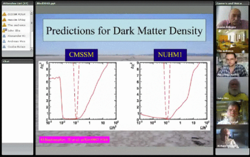
Figure 21: Videoconference Bled-Marburg-Liege-Geneve-Moscow-Australia with lecture by John Ellis, which he gave from his office in CERN, Switzerland, became a part of the program of XIII Bled Workshop.

The ppt or pdf file of presentation is uploaded in the system in advance and then demonstrated in the central window. Video images of presenter and participants appear in the right window, while in the lower left window the list of all the attendees is given. To protect the quality of sound and record, the participants are required to switch out their audio system during presentation and to use upper left Chat window for immediate comments and urgent questions. The Chat window can be also used by participants, having no microphone, for questions and comments during Discussion. In the end of presentation the central window can be used for a whiteboard utility as well as the whole structure of windows can be changed, e.g. by making full screen the window with the images of participants of discussion.

0.84 VIA Sessions at Bled Workshop

0.84.1 The program of discussions

In the course of Bled Workshop meeting the list of open questions was stipulated, which was proposed for wide discussion with the use of VIA facility (see mkVIAnorma ).

The list of these questions was put on the VIA site and all the participants of VIA sessions were invited to address them during VIA discussions. Some of them were covered in the VIA lectures (see their records in mkVIAVIAbled ):

• ”Is the ”Approach unifying spins and charges” into only two kinds of the spin offering the right answers to the open questions of the standard models?” by Norma Mankoc-Borstnik (in two parts )

• ”Arguments for there being Backward Causation, funny coincidences.” by Holger Bech Nielsen (in two parts)

• ”Atoms of dark matter from new stable charged particles” by Maxim Khlopov

• ”New LHC Light on Dark Matter” by John Ellis

The use of the sensitive audio system KONFTEL 300W mkVIAkonftel supported VIA discussions inside the Bled conference room in the way most natural for the non-formal atmosphere of Bled Workshops. The advantage of the interactivity of VIA system has provided distant participants to share this atmosphere and contribute the discussion. The important refinement of adobe Connect system is that it is possible now to use pdf files, what facilitated VIA presentations by N.S. Mankoč Borštnik and Holger Bech Nielsen (see and image form the latter videoconference on Fig. 22).

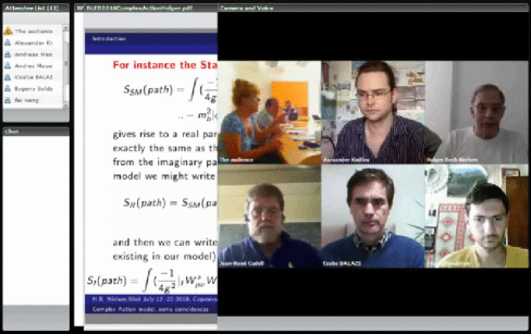
Figure 22: Videoconference with VIA talk by Holger Bech Nielsen

0.84.2 VIA discussions

VIA discussion sessions of XIII Bled Workshop have developed from the first experience at XI Bled Workshop mkVIABregar:2008zz and their more regular practice at XII Bled Workshop mkVIABledVIA . They became a regular part of the Workshop’s programme.

In the framework of the program of Bled Workshop John Ellis, staying in his office in CERN, gave his talk ”New LHC Light on Dark Matter” and took part in the successive discussion. VIA sessions were finished by the discussion of puzzles of dark matter searches (see mkVIABled ). N.S. Mankoč Borštnik presented possible dark matter candidates that follow from the approach, unifying spins and charges, and Maxim Khlopov presented composite dark matter scenario, mentioning that it can offer the solution for the puzzles of direct dark matter searches as well as that it can find physical basis in the above approach. The comments by Rafael Lang from his office in USA were very important for clarifying the current status of experimental constraints on the possible properties of dark matter candidates (Fig. 23)

VIA sessions provided participation at distance in Bled discussions for John Ellis (CERN, Switezerland), K.Belotsky, N.Chasnikov, A.Mayorov and E. Soldatov (MEPhI, Moscow), J.-R. Cudell (Liege, Belgium), R.Weiner (Marburg, Germany) C. Balasz (Australia) and many others.

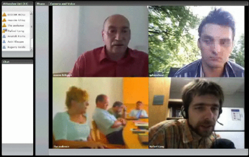
Figure 23: Bled Conference Discussion Bled-Moscow-CERN-Norge-Marburg-Liege-USA

0.85 Conclusions

Current VIA activity is integrated in the structure of APC laboratory and includes regular weekly videoconferences with VIA lectures, online transmissions of APC Colloquiums and Seminars, a solid library of their records and presentations, work of multi-lingual VIA Internet forum.

The Scientific-Educational complex of Virtual Institute of Astroparticle physics can provide regular communications between different groups and scientists, working in different scientific fields and parts of the world, get the first-hand information on the newest scientific results, as well as to support various educational programs on distance. This activity would easily allow finding mutual interest and organizing task forces for different scientific topics of astroparticle physics and related topics. It can help in the elaboration of strategy of experimental particle, nuclear, astrophysical and cosmological studies as well as in proper analysis of experimental data. It can provide young talented people from all over the world to get the highest level education, come in direct interactive contact with the world known scientists and to find their place in the fundamental research.

VIA sessions became a natural part of a program of Bled Workshops, opening the room of discussions of physics beyond the Standard Model for distant participants from all the world.

References

-
(1)
R.J. Szabo, Quantum Field Theory on Noncommutative
Spaces, Phys. Rept. 378 (2003) 207 [hep-th/0109162];
R.J. Szabo, Discrete Noncommutative Gauge Theory, Mod. Phys. Lett. A16 (2001) 367 [hep-th/0101216]. -
(2)
W. Bietenholz, F. Hofheinz, J. Nishimura, Non-Commutative Field Theories beyond Perturbation
Theory, Fortsch. Phys. 51 (2003) 745 [hep-th/0212258];
W. Bietenholz, F. Hofheinz, J. Nishimura, Y. Susaki, J. Volkholz, First Simulation Results for the Photon in a Non-Commutative Space, Nucl. Phys. Proc. Suppl. 140 (2005) 772 [hep-lat/0409059];
W. Bietenholz, A. Bigarini, F. Hofheinz, J. Nishimura, Y. Susaki, J. Volkholz, Numerical Results for U() Gauge Theory on 2d and 4d Non-Commutative Spaces, Fortsch. Phys. 53 (2005) 418 [hep-th/0501147]. -
(3)
H. Aoki, J. Nishimura, Y. Susaki, The Index of the Overlap
Dirac Operator on a Discretized 2d Non-Commutative Torus, J. High Energy
Phys. 02 (2007) 033 [hep-th/0602078];
H. Aoki, J. Nishimura, Y. Susaki, Probability Distribution of the Index in Gauge Theory on 2d Non-Commutative Geometry, J. High Energy Phys. 10 (2007) 024 [hep-th/0604093];
H. Aoki, J. Nishimura, Y. Susaki, Finite-Matrix Formulation of Gauge Theories on a Non-Commutative Torus with Twisted Boundary Conditions, J. High Energy Phys. 04 (2009) 055 [arXiv:0810.5234];
H. Aoki, J. Nishimura, Y. Susaki, Dominance of a Single Topological Sector in Gauge Theory on Non-Commutative Geometry, J. High Energy Phys. 09 (2009) 084 [arXiv:0907.2107]. -
(4)
W. Frisch, H. Grosse, H. Markum, Instantons in
Two-Dimensional Noncommutative U(1) Gauge Theory,
PoS(LATTICE 2007)317;
R. Achleitner, W. Frisch, H. Grosse, H. Markum, F. Teischinger, Topology of Noncommutative U(1) Gauge Theory on the Lattice, Bled Workshops in Physics 8,1 (2007) 43. - (5) A. González-Arroyo, M. Okawa, A Twisted Model for Large- Lattice Gauge Theory, Phys. Rev. D27 (1983) 2397.
- (6) T. Eguchi, H. Kawai, Reduction of Dynamical Degrees of Freedom in the Large-N Gauge Theory, Phys. Rev. Lett. 48 (1982) 1063.
- (7) L. Griguolo, D. Seminara, Classical Solutions of the TEK Model and Noncommutative Instantons in Two Dimensions, J. High Energy Phys. 03 (2004) 068 [hep-th/0311041].
-
(8)
W. Bietenholz, J. Nishimura, Y. Susaki, J. Volkholz,
A Non-Perturbative Study of 4d U(1) Non-Commutative Gauge Theory –
the Fate of One-Loop Instability, J. High Energy Phys. 10 (2006) 042
[hep-th/0608072];
J. Nishimura, W. Bietenholz, Y. Susaki, J. Volkholz, A Non-Perturbative Study of Non-Commutative U(1) Gauge Theory [arXiv:0706.3244].

References

- (1) J. J. Sakurai, Advanced Quantum Mechanics. (Addison-Wesley, 1967).
- (2) L. H. Ryder, Quantum Field Theory. (Cambridge University Press, Cambridge, 1985).
- (3) C. Itzykson and J.-B. Zuber, Quantum Field Theory. (McGraw-Hill Book Co., 1980), p. 156.
- (4) V. V. Dvoeglazov, Int. J. Theor. Phys. 34 (1995) 2467; Nuovo Cim. 108A (1995) 1467, Hadronic J. 20 (1997) 435; Acta Phys. Polon. B29 (1998) 619.
- (5) V. V. Dvoeglazov, Mod. Phys. Lett. A12 (1997) 2741.
- (6) V. V. Dvoeglazov, Int. J. Theor. Phys. 43 (2004) 1287.
- (7) A. O. Barut, Phys. Lett. 73B (1978) 310; Phys. Rev. Lett. 42 (1979) 1251.
- (8) E. Majorana, Nuovo Cimento 14 (1937) 171.
- (9) S. M. Bilenky and B. M. Pontekorvo, Phys. Repts 42 (1978) 224.
- (10) E. P. Wigner, Ann. Math. 40 (1939) 149; S. Weinberg, Phys. Rev. 133 (1964) B1318.
- (11) R. N. Faustov, Preprint ITF-71-117P, Kiev, Sept.1971.
- (12) A. Barut and G. Ziino, Mod. Phys. Lett. A8 (1993) 1099; G. Ziino, Int. J. Mod. Phys. A11 (1996) 2081.
- (13) D. V. Ahluwalia, Int. J. Mod. Phys. A11 (1996) 1855.
- (14) P. Lounesto, Clifford Algebras and Spinors. (Cambridge University Press, 2002), Ch. 11 and 12; R. da Rocha and W. Rodrigues, Jr., Where are Elko Spinor Fields in Lounesto Spinor Field Classification? Preprint math-ph/0506075.
- (15) M. Kirchbach, C. Compean and L. Noriega, Beta Decay with Momentum-Space Majorana Spinors. Eur. Phys. J. A22 (2004) 149.
- (16) M. Markov, ZhETF 7 (1937), 579, 603; Nucl. Phys. 55 (1964) 130.
- (17) I. M. Gelfand and M. L. Tsetlin, ZhETF 31 (1956) 1107; G. A. Sokolik, ZhETF 33 (1957) 1515.
- (18) B. Nigam and L. L. Foldy, Phys. Rev. 102 (1956) 1410.
- (19) V. B. Berestetskii, E. M. Lifshitz and L. P. Pitaevskii, Quantum Electrodynamics.The IV Volume of the Landau Course of Theoretical Physics. 2nd Edition (Butterworth-Heinemann, 1982).
- (20) A. Gersten, Found. Phys. Lett. 12 (1999) 291.
- (21) V. V. Dvoeglazov, J. Phys. A33 (2000) 5011; Rev. Mex. Fis. Supl. 49-S1 (2003) 99.
- (22) K. R. Brownstein, Am. J. Phys. 67 (1999) 639.
- (23) V. V. Dvoeglazov, Proc. the ICSSUR 2003 Conference, Puebla, México, June 2003 (Rinton Press, 2003), pp. 125-130, math-ph/0308017.
- (24) V. V. Dvoeglazov, Fizika B6 (1997) 111.
- (25) A. Barut, I. Muzinich and D. N. Williams, Phys. Rev. 130 (1963) 442.
- (26) A. Sankaranarayanan and Good, jr, Nuovo Cimento 36 (1965) 1303.
- (27) D. L.Weaver, C. L. Hammer and R. H. Good, jr., Phys. Rev. B135 (1964) 241.
- (28) D. V. Ahluwalia, M. B. Johnson and T. Goldman, Phys. Lett. B316 (1993) 102.
- (29) R. H. Tucker and C. L. Hammer, Phys. Rev. D3 (1971) 2448.
- (30) N. N. Bogoliubov and D. V. Shirkov, Introduction to the Theory of Quantized Fields. 3rd Edition. (Nauka, Moscow, 1973), p.28, p, 55.

References

- (1) V. Bargmann and E. Wigner, Proc. Nat. Acad. Sci. 34 (1948) 211.
- (2) D. Luriè, Particles and Fields (Interscience Publishers, 1968), Chapter 1.
- (3) V. V. Dvoeglazov, Hadronic J. 25 (2002) 137, hep-th/0112111; ibid. 26 (2003) 299, hep-th/0208159.
- (4) V. V. Dvoeglazov, Phys. Scripta 64 (2001) 201.
- (5) V. V. Dvoeglazov, Adv. Appl. Clifford Algebras 10 (2000) 7.

References

- (1) M. Bustamante, L. Cieri and J. Ellis, arXiv:0911.4409 [hep-ph]; in Proceedings of the 2009 CERN-Latin-American School of High-Energy Physics, Recinto Quirama, Colombia, 15 - 28 March 2009, eds. C. Grojean and M. Spiropulu, arXiv:1010.5976 [hep-ph].
- (2) G. Servant and T. M. P. Tait, Nucl. Phys. B 650 (2003) 391 [arXiv:hep-ph/0206071].
- (3) H. C. Cheng and I. Low, JHEP 0309 (2003) 051 and JHEP 0408 (2004) 061.
- (4) J. Ellis, J.S. Hagelin, D.V. Nanopoulos, K.A. Olive and M. Srednicki, Nucl. Phys. B 238 (1984) 453; see also H. Goldberg, Phys. Rev. Lett. 50 (1983) 1419.
- (5) L. Maiani, All You Need To Know About The Higgs Boson, Proceedings of the Gif-sur-Yvette Summer School On Particle Physics, 1979, pp.1-52; G. ’t Hooft, in Recent developments in Gauge Theories, Proceedings of the NATO Advanced Study Institute, Cargèse, 1979, eds. G. ’t Hooft et al. (Plenum Press, NY, 1980); E. Witten, Phys. Lett. B 105 (1981) 267.
- (6) ALEPH, CDF, D0, DELPHI, L3, OPAL and SLD Collaborations, LEP and Tevatron Electroweak Working Groups, SLD Electroweak and Heavy Flavour Groups, arXiv:0911.2604.
- (7) J. Ellis, S. Kelley and D.V. Nanopoulos, Phys. Lett. 260 (1991) 131; U. Amaldi, W. de Boer and H. Furstenau, Phys. Lett. B260 (1991) 447; P. Langacker and M. Luo, Phys. Rev. D44 (1991) 817; C. Giunti, C. W. Kim and U. W. Lee, Mod. Phys. Lett. A 6 (1991) 1745.
- (8) H. P. Nilles, Phys. Rept. 110, 1 (1984); H. E. Haber and G. L. Kane, Phys. Rept. 117, 75 (1985). S. P. Martin, A Supersymmetry Primer, arXiv:hep-ph/9709356.
- (9) J. R. Ellis, K. A. Olive, Y. Santoso and V. C. Spanos, Phys. Rev. D 70, 055005 (2004) [arXiv:hep-ph/0405110].
- (10) J. R. Ellis, K. A. Olive and P. Sandick, Phys. Lett. B 642, 389 (2006) [arXiv:hep-ph/0607002];
- (11) J. Ellis, A. Mustafayev and K. A. Olive, Eur. Phys. J. C 69 (2010) 201 [arXiv:1003.3677 [hep-ph]].
- (12) J. R. Ellis and D. V. Nanopoulos, Phys. Lett. B 110 (1982) 44.
- (13) Joint Supersymmetry Working Group of the ALEPH, DELPHI, L3 and OPAL experiments, http://lepsusy.web.cern.ch/lepsusy/.
- (14) K. Nakamura et al. (Particle Data Group), J. Phys. G 37, 075021 (2010).
- (15) S. Schael et al. [ALEPH, DELPHI, L3, OPAL Collaborations and LEP Working Group for Higgs boson searches], Eur. Phys. J. C 47 (2006) 547 [arXiv:hep-ex/0602042].
- (16) G. W. Bennett et al. [Muon g-2 Collaboration], Phys. Rev. Lett. 92 (2004) 161802 [arXiv:hep-ex/0401008].
- (17) E. Komatsu et al., arXiv:1001.4538 [astro-ph.CO] and references therein.
- (18) M. Davier, A. Hoecker, B. Malaescu, C. Z. Yuan and Z. Zhang, arXiv:0908.4300 [hep-ph].
- (19) M. Davier, A. Hoecker, B. Malaescu and Z. Zhang, arXiv:1010.4180 [hep-ph].
- (20) J. R. Ellis, K. A. Olive, Y. Santoso and V. C. Spanos, Phys. Lett. B 565, 176 (2003) [arXiv:hep-ph/0303043].
- (21) O. Buchmueller et al., Phys. Lett. B 657 (2007) 87 [arXiv:0707.3447 [hep-ph]].
- (22) O. Buchmueller et al., JHEP 0809 (2008) 117 [arXiv:0808.4128 [hep-ph]].
- (23) O. Buchmueller et al., Eur. Phys. J. C 64 (2009) 391 [arXiv:0907.5568 [hep-ph]].
- (24) M. W. Goodman and E. Witten, Phys. Rev. D 31 (1985) 3059.
- (25) M. Srednicki, K. A. Olive and J. Silk, Nucl. Phys. B 279 (1987) 804.
- (26) See, for example, P. Scott, J. Conrad, J. Edsjo, L. Bergstrom, C. Farnier and Y. Akrami, JCAP 1001 (2010) 031 [arXiv:0909.3300 [astro-ph.CO]] and references therein.
- (27) J. Silk and M. Srednicki, Phys. Rev. Lett. 53 (1984) 624.
- (28) Z. Ahmed et al. [The CDMS-II Collaboration], Science 327 (2010) 1619 [arXiv:0912.3592 [astro-ph.CO]].
- (29) E. Aprile et al. [XENON100 Collaboration], Phys. Rev. Lett. 105 (2010) 131302 [arXiv:1005.0380 [astro-ph.CO]].
- (30) R. Bernabei et al., arXiv:1007.0595 [astro-ph.CO].
- (31) C. E. Aalseth et al. [CoGeNT collaboration], arXiv:1002.4703 [astro-ph.CO].
- (32) J. R. Ellis, K. A. Olive and C. Savage, Phys. Rev. D 77 (2008) 065026 [arXiv:0801.3656 [hep-ph]].
- (33) J. Ellis, K. A. Olive, C. Savage and V. C. Spanos, Phys. Rev. D 81 (2010) 085004 [arXiv:0912.3137 [hep-ph]].
-
(34)
R. Gaitskell and J. Filippini,
http://dmtools.berkeley.edu/
slimitplots/ . - (35) Z. Ahmed et al. [CDMS Collaboration], Phys. Rev. Lett. 102 (2009) 011301 [arXiv:0802.3530 [astro-ph]].
- (36) J. Angle et al., Phys. Rev. Lett. 101 (2008) 091301 [arXiv:0805.2939 [astro-ph]].
- (37) SuperCDMS Development Project, Fermilab Proposal 0947, October 2004.
- (38) J. Ahrens et al. [IceCube Collaboration], Astropart. Phys. 20, 507 (2004) [arXiv:astro-ph/0305196].
-
(39)
See, for example
T. Le Compte, Talk at the 103rd Open Session of the LHCC,
http://indico.cern.ch/getFile.py/access?contribId=2
&resId=1&materialId=slides&confId=105780. -
(40)
ATLAS Collaboration, http://cdsweb.cern.ch/record/1278474/
files/ATL-PHYS-PUB-2010-010.pdf; see also
CMS Collaboration, CMS-NOTE-2010-008, https://twiki.cern.ch/
twiki/bin/view/CMSPublic/PhysicsResultsSUS.

References

- (1) R. Erdem, A symmetry for vanishing cosmological constant in an extra dimensional toy model, Phys. Lett. B 621, 11 (2005), hep-th/0410063
- (2) S. Weinberg, The Quantum Theory of Fields, Vol. I, chapter 5 (Cambridge Univ. Press, New York, 1995)
- (3) S. Nobbenhuis, Categorizing different approaches to the cosmological constant problem, Found. Phys. 36, 613 (2006), gr-qc/0411093
- (4) G. ’t Hooft, S. Nobbenhuis, Invariance under complex transformations, and its relevance to the cosmological constant problem, Class. Quant. Grav. 23, 3819 (2006)
- (5) G. Bonelli, A. Boyarsky, Six-dimensional topological gravity and the cosmological constant problem, Phys. Lett. B 490, 147 (2000), hep-th/0004058
- (6) R. Erdem, A symmetry for vanishing cosmological constant: Another realization, Phys. Lett. B 639, 348 (2006), gr-qc/0603080
- (7) M.J. Duff, J. Kalkkinen, Signature reversal invariance, Nucl. Phys. B 758, 161 (2006)
- (8) R. Erdem, A symmetry for vanishing cosmological constant, J. Phys. A 40, 6945 (2007), gr-qc/0611111
- (9) R. Erdem, A way to get rid of cosmological constant and zero-point energy problems of quantum fields through metric reversal symmetry, J. Phys. A 41, 235401 (2008), arXiv:0712.2989
- (10) R. Erdem, Finite number of Kaluza-Klein modes, all with zero masses, Mod. Phys. Lett. A 25, 825 (2010), arXiv:0809.2647
- (11) R. Erdem, Possibility of automatic Pauli-Villars-like regularization through extra dimensions, preprint, arXiv:0902.4819
- (12) M.J. Duff, Kaluza-Klein theory in perspective, in Stockholm 1994, The Oskar Klein centenary pp 22-35, preprint Arxiv hep-th/9410046
- (13) P. Di Francesco, P. Mathieu, D. Sénéchal, Conformal Field Theory, pp. 168-171 (Springer, New York, 1997)
- (14) W. Pauli and F. Villars, On the Invariant Regularization in Quantum Field Theory, Rev. Mod. Phys. 21, 434 (1949)

References

- (1) S. Weinberg, Phys. Rev. Lett.29, 388(1972); H. Georgi and S.L. Glashow, Phys. Rev. D 7, 2457(1973); R.N. Mohapatra, Phys. Rev. D 9, 3461(1974); S.M. Barr and A. Zee, Phys. Rev. D 15, 2652(1977); H. Georgi, ”Fermion Masses in Unified models”, in First Workshop in Grand Unification, ed. P.H. Frampton, S.L. Glashow, and A. Yildiz(1980, Math Sci Press, Brookline, MA); S.M. Barr ,Phys. Rev. D 21, 1424(1980); R. Barbieri and D.V. Nanopoulos, Phys. Lett. B 95, 43(1980); S.M. Barr ,Phys. Rev. D 24, 1895(1981); L.E. Ibanez, Phys. Lett. B 177, 403(1982); B.S. Balakrishna, A.L. Kagan and R.N. Mohapatra, Phys. Lett. B 205, 345(1988); B.S. Balakrishna, Phys. Rev. Lett. 60, 1602(1988); K.S. Babu and E. Ma, Mod. Phys. Lett. A 4 , 1975(1989); H.P. Nilles, M. Olechowski and S. Pokorski, Phys. Lett. B 248, 378(1990); R. Rattazzi, Z. Phys.C 52, 575(1991); K.S. Babu and R.N. Mohapatra, Phys. Rev. Lett. 64, 2747(1990); X.G. He, R.R. Volkas, and D.D. Wu, Phys. Rev. D 41, 1630(1990); Ernest Ma, Phys. Rev. Lett. 64 (1990) 2866. B.A. Dobrescu and P.J. Fox, JHEP 0808, 100(2008); S.M. Barr, Phys. Rev. D 76, 105024(2007); S.M. Barr and A. Khan, Phys. Rev. D 79, 115005(2009);
- (2) Sandip Pakvasa and Hirotaka Sugawara, Phys. Lett. B 73 61(1978); Y. Yamanaka, H. Sugawara, and S. Pakvasa, Phys. Rev. D 25 1895(1982); K. S. Babu and X.G. He, ibid. 36 3484(1987); Ernest Ma, Phys. Rev. Lett. B 62 61(1989).
- (3) A. Davidson, M. Koca, and K. C. Wali, Phys. Rev. Lett. B 43 92(1979), Phys. Rev. D 20 1195(1979); C. D. Froggatt and H. B. Nielsen, Nucl. Phys. B 147 277(1979); A. Sirlin, Phys. Rev. D 22 971(1980); A. Davidson and K. C. Wali, ibid. 21 787(1980).
- (4) X.G. He, R. R: Volkas, and D. D. Wu, Phys. Rev. D 41 1630(1990); Ernest Ma, Phys. Rev. Lett. 64 2866(1990).
- (5) E. Garcia, A. Hernandez-Galeana, D. Jaramillo, W. A. Ponce and A. Zepeda, Revista Mexicana de Fisica Vol. 48(1), 32(2002); E. Garcia, A. Hernandez-Galeana, A. Vargas and A. Zepeda, hep-ph/0203249.
- (6) N. Chen, T. A. Ryttov, and R. Shrock, arXiv:1010.3736 [hep-ph]; C. T. Hill and E. H. Simmons, Phys. Rept. 381, 235 (2003); Workshop on Dynamical Electroweak Symmetry Breaking, Southern Denmark Univ. 2008 (http://hep.sdu.dk/dewsb); R.S. Chivukula, M. Narain, and J. Womersley, in Particle Data Group, J. Phys. G 37 1340, (2010); F. Sannino, Acta Phys. Polon. B 40, 3533 (2009)(arXiv:0911.0931).
- (7) A. Hernandez-Galeana, Rev. Mex. Fis. Vol. 50(5), (2004) 522. hep-ph/0406315.
- (8) A. Hernandez-Galeana, Bled Workshops in Physics, Vol. 10, No. 2, (2009) 67; arXiv:0912.4532
-
(9)
For review and some recent works see for example:
B. Holdom, W.S. Hou, T. Hurth, M. Mangano, S. Sultansoy and G. Unel, ”Beyond the 3-generation SM in the LHC era” Workshop, CERN, September 4-5, 2008; arXiv:0904.4698 and references therein. - (10) N.S. Mankoč Borštnik, this Volume, p. 0.37.
- (11) M. Y. Khlopov, A. G. Mayorov, and E. Y. Soldatov, this Volume, p. 0.28 and p. 0.67.
- (12) Jonathan M. Arnold, Bartosz Fornal and Michael Trott; arXiv:1005.2185 and references therein.
- (13) T. Yanagida, Phys. Rev. D 20, 2986 (1979).
- (14) A.Hernandez-Galeana, Phys.Rev. D 76, 093006(2007).
- (15) K. Nakamura et al., Particle Data Group, J. Phys. G: Nucl. Part. Phys. 37 (2010) 075021.

References

- (1) M.Yu. Khlopov Cosmoparticle physics (World Scientific, Singapore, 1999).
- (2) M.Yu. Khlopov in Cosmion-94, Eds. M.Yu.Khlopov et al. (Editions frontieres, 1996) P. 67; M. Y. Khlopov in hep-ph/0612250 , p 51.
- (3) M. Y. Khlopov in arXiv:0711.4681, p. 114; M. Y. Khlopov and N. S. Mankoc-Borstnik, ibid, p. 195.
- (4) L. B. Okun, Phys. Usp. 50 (2007) 380 [arXiv:hep-ph/0606202].
- (5) A. G. Polnarev and M. Y. Khlopov, Sov. Phys. Usp. 28, 213 (1985) [Usp. Fiz. Nauk 145, 369 (1985)]; M. Y. Khlopov, Res. Astron. Astrophys. 10, 495 (2010) [arXiv:0801.0116 [astro-ph]].
- (6) D. C. Dai, K. Freese and D. Stojkovic, JCAP 0906 (2009) 023 [arXiv:0904.3331 [hep-ph]].
- (7) S. L. Glashow, arXiv:hep-ph/0504287.
- (8) D. Fargion and M. Khlopov, arXiv:hep-ph/0507087.
- (9) K.M.Belotsky et al, Gravitation and Cosmology 11, 3 (2005)
- (10) M.Yu. Khlopov, JETP Lett. 83, 1 (2006).
- (11) K. Belotsky et al, arXiv:astro-ph/0602261. K. Belotsky et al, Gravitation and Cosmology 12, 1 (2006); K. Belotsky et al, arXiv:0806.1067 [astro-ph].
- (12) M. Y. Khlopov, arXiv:astro-ph/0607048.
- (13) C. A. Stephan, arXiv:hep-th/0509213.
- (14) D. Fargion et al, Class. Quantum Grav. 23, 7305 (2006); M. Y. Khlopov and C. A. Stephan, arXiv:astro-ph/0603187.
- (15) A. Connes Noncommutative Geometry (Academic Press, London and San Diego, 1994). M. Y. Khlopov and C. A. Stephan, arXiv:astro-ph/0603187.
- (16) M. Y. Khlopov and C. Kouvaris, Phys. Rev. D 77, 065002 (2008).
- (17) F. Sannino and K. Tuominen, Phys. Rev. D 71, 051901 (2005); D. K. Hong et al, Phys. Lett. B 597, 89 (2004); D. D. Dietrich et al, Phys. Rev. D 72, 055001 (2005); D. D. Dietrich et al, arXiv:hep-ph/0510217; S. B. Gudnason et al, Phys. Rev. D 73, 115003 (2006); S. B. Gudnason et al, Phys. Rev. D 74, 095008 (2006).
- (18) N.S. Mankoč Borštnik, this Volume, p. 0.37; A. Borštnik Bračič, N.S. Mankoč Borštnik, Phys. Rev. D 74, 073013 (2006); N.S. Mankoč Borštnik, Mod. Phys. Lett. A 10, 587 (1995); N.S. Mankoč Borštnik, Int. J. Theor. Phys. 40, 315 (2001); G. Bregar, M. Breskvar, D. Lukman, N.S. Mankoč Borštnik, New J. of Phys. 10, 093002 (2008).
- (19) M. Y. Khlopov and C. Kouvaris, Phys. Rev. D 78, 065040 (2008)
- (20) M. Y. Khlopov, AIP Conf. Proc. 1241 (2010) 388 [arXiv:0911.5685 [astro-ph.CO]].
- (21) M. Y. Khlopov, A. G. Mayorov and E. Y. Soldatov, Int. J. Mod. Phys. D 19 (2010) 1385 [arXiv:1003.1144 [astro-ph.CO]].
- (22) M. Y. Khlopov, arXiv:0806.3581 [astro-ph].
- (23) C. B. Dover et al, Phys. Rev. Lett. 42, 1117 (1979); S. Wolfram, Phys. Lett. B 82, 65 (1979); G. D. Starkman et al, Phys. Rev. D 41, 3594 (1990); D. Javorsek et al, Phys. Rev. Lett. 87, 231804 (2001); S. Mitra, Phys. Rev. D 70, 103517 (2004); G. D. Mack et al, Phys. Rev. D 76, 043523 (2007);
- (24) B. D. Wandelt et al., arXiv:astro-ph/0006344; P. C. McGuire and P. J. Steinhardt, arXiv:astro-ph/0105567; G. Zaharijas and G. R. Farrar, Phys. Rev. D 72, 083502 (2005)
- (25) M. Y. Khlopov, arXiv:0801.0167 [astro-ph]; M. Y. Khlopov, arXiv:0801.0169 [astro-ph].
- (26) M. Y. Khlopov, A. G. Mayorov and E. Y. Soldatov, “Puzzles of Dark Matter - More Light on Dark Atoms?”, this Volume, p. 0.67.
- (27) K.M.Belotsky, A.G.Mayorov, M.Yu.Khlopov. Charged particles of dark matter in cosmic rays. ISBN 978-5-7262-1280-7, Scientific Session NRNU MEPhI-2010, V.4, P.127
- (28) D. P. Finkbeiner and N. Weiner, Phys. Rev. D 76, 083519 (2007)
- (29) B. J. Teegarden et al, Astrophys. J. 621, 296 (2005)
- (30) D. McCammon et al, Nucl. Instrum. Methods A 370, 266 (1996); D. McCammon et al, Astrophys. J. 576, 188 (2002).
- (31) K. Belotsky et al, arXiv:astro-ph/0606350.
- (32) D. S. Akerib et al. [CDMS Collaboration], Phys. Rev. Lett. 96, 011302 (2006); Z. Ahmed et al. [CDMS Collaboration], arXiv:0802.3530 [astro-ph]. N. Mirabolfathi et al. [CDMS Collaboration], Nucl. Instrum. Methods A 559, 417 (2006);
- (33) R. N. Cahn and S. L. Glashow, Science 213, 607 (1981); M. Pospelov, Phys. Rev. Lett. 98, 231301 (2007); K. Kohri and F. Takayama, Phys. Rev. D 76, 063507 (2007).
- (34) M. Yu. Khlopov, A. G. Mayorov, E.Yu. Soldatov, Bled Workshops in Physics 10, 79 (2009); arXiv:0911.5606.
- (35) R. Bernabei et al., Rivista Nuovo Cimento 26, 1 (2003)
- (36) R. Bernabei et al. [DAMA Collaboration], Eur.Phys.J C56, 333 (2008) arXiv:0804.2741 [astro-ph].
- (37) L. D. Landau, E. M. Lifshitz Quantum Mechanics: Non-Relativistic Theory (Fizmatlit, Moscow, 2004).
- (38) R. Bernabei et al. [DAMA Collaboration], Nucl. Instrum. Meth. A 592 (2008) 297 [arXiv:0804.2738 [astro-ph]].
- (39) A. b. A. Dadi, Phys. Rev. C 82 (2010) 025203 [arXiv:1005.2030 [nucl-th]].
- (40) Yu. A. Troyan, A. V. Beljaev, A. Y. Troyan, E. B. Plekhanov, A. P. Jerusalimov and S. G. Arakelian, arXiv:1011.3124 [hep-ex].
- (41) F. Petriello and K. M. Zurek, JHEP 0809, 047 (2008); R. Foot, Phys. Rev. D 78, 043529 (2008); J. L. Feng, J. Kumar and L. E. Strigari, arXiv:0806.3746 [hep-ph]; J. L. Feng, J. Kumar, J. Learned and L. E. Strigari, arXiv:0808.4151 [hep-ph]; E. M. Drobyshevski, arXiv:0811.0151 [astro-ph]; B. Feldstein, A. L. Fitzpatrick and E. Katz, JCAP 1001 (2010) 020 [arXiv:0908.2991 [hep-ph]]; Y. Bai and P. J. Fox, JHEP 0911 (2009) 052 [arXiv:0909.2900 [hep-ph]]; B. Feldstein, A. L. Fitzpatrick, E. Katz and B. Tweedie, JCAP 1003 (2010) 029 [arXiv:0910.0007 [hep-ph]]; A. L. Fitzpatrick, D. Hooper and K. M. Zurek, Phys. Rev. D 81 (2010) 115005 [arXiv:1003.0014 [hep-ph]]; S. Andreas, C. Arina, T. Hambye, F. S. Ling and M. H. G. Tytgat, Phys. Rev. D 82 (2010) 043522 [arXiv:1003.2595 [hep-ph]]; D. S. M. Alves, S. R. Behbahani, P. Schuster and J. G. Wacker, JHEP 1006 (2010) 113 [arXiv:1003.4729 [hep-ph]]; V. Barger, M. McCaskey and G. Shaughnessy, Phys. Rev. D 82 (2010) 035019 [arXiv:1005.3328 [hep-ph]]; C. Savage, G. Gelmini, P. Gondolo and K. Freese, arXiv:1006.0972 [astro-ph.CO]; D. Hooper, J. I. Collar, J. Hall and D. McKinsey, arXiv:1007.1005 [hep-ph]; S. Chang, R. F. Lang and N. Weiner, arXiv:1007.2688 [hep-ph]; S. Chang, N. Weiner and I. Yavin, arXiv:1007.4200 [hep-ph]; V. Barger, W. Y. Keung and D. Marfatia, arXiv:1007.4345 [hep-ph]. A. L. Fitzpatrick and K. M. Zurek, arXiv:1007.5325 [hep-ph]; T. Banks, J. F. Fortin and S. Thomas, arXiv:1007.5515 [hep-ph]; B. Feldstein, P. W. Graham and S. Rajendran, arXiv:1008.1988 [hep-ph].
- (42) G. B. Gelmini, Int. J. Mod. Phys. A 23 (2008) 4273 [arXiv:0810.3733 [hep-ph]]; E. Aprile, S. Profumo, New J. Phys. 11 (2009) 105002; J. L. Feng, arXiv:1003.0904 [astro-ph.CO].

References

- (1) N.S. Mankoč Borštnik, Phys. Lett. B 292 (1992) 25-29, Int. J. Theor. Phys. 40 (2001) 315-337, hep-ph/0711.4681, 94-113, J. Math. Phys. 34 (1993) 3731-3745, Mod. Phys. Lett. A 10 (1995) 587-595.
- (2) A. Borštnik Bračič, N.S. Mankoč Borštnik, hep-ph/0512062, Phys. Rev. D 74 (2006) 073013-16.
- (3) C.G. Callan, R.F. Dashen, D.J. Gross, Phys. Lett. 63 B (1976) 334.
- (4) V.A. Rubakov, M.E. Shaposhnikov, Phys.Usp. 39 (1996) 461-502, arxiv:hep-ph/9603208v2.
- (5) M. Dine, A. Kusenko, Rev.Mod.Phys. 76 (2004) 1, arxiv:hep-ph/0303065v3.
- (6) Ta-Pei Cheng, Ling-Fong Li, Gauge theory of elementary particle physics, Clarendon Press, Oxford (1986)
- (7) N.S. Mankoč Borštnik, H. B. Nielsen, Phys. Lett. B 633 (2006) 771-775, hep-th/0311037, hep-th/0509101, arXiv:1001.4679v3.
- (8) G. Bregar, M. Breskvar, D. Lukman, N.S. Mankoč Borštnik, New J. of Phys. 10 (2008) 093002, hep-ph/07082846.
- (9) N.S. Mankoč Borštnik, this Volume, p. 0.37.
- (10) G. Bregar, N.S. Mankoč Borštnik, Phys. Rev. 80 (2009) 083534, arXiv:0907.0196v1.
- (11) The work in progress.
- (12) A. Hernández-Galeana, N.S. Mankoč Borštnik, this Volume, p. 0.61.
- (13) M.Yu. Khlopov, N.S. Mankoč Borštnik, this Volume, p. 0.64.
- (14) M.Yu. Khlopov et al, this Volume, p. 0.28.
- (15) N.S. Mankoč Borštnik, J. of Math. Phys. 34 (1993) 3731, N.S. Mankoč Borštnik, H.B. Nielsen, J. of Math. Phys. 43 (2002) 5782, hep-th/0111257, J. of Math. Phys. 44 (2003) 4817, hep-th/0303224.
- (16) A. Borštnik bračič, N.S. Mankoč Borštnik, hep-ph/0401043, p. 31-57.

References

- (1) N.S. Mankoč Borštnik, Phys. Lett. B 292 (1992) 25, J. Math. Phys. 34 (1993) 3731 Int. J. Theor. Phys. 40 315 (2001), Modern Phys. Lett. A 10 (1995) 587, Proceedings of the Lomonosov conference on Elementary Physics Particle physics in the EVE of LHC, World Scientific, (2009) p. 371-378, hep-ph/0711.4681 p.94, arXiv:0912.4532 p.119.
- (2) A. Borštnik, N.S. Mankoč Borštnik, hep-ph/0401043, hep-ph/0401055, hep-ph/0301029, Phys. Rev. D 74 (2006) 073013, hep-ph/0512062.
- (3) N.S. Mankoč Borštnik, hep-ph/0711.4681, p. 94-113, http://viavca.in2p3.fr, arxiv:0812.0510[hep-ph],1-12, arXiv:0912.4532, p.119-135.
- (4) N.S. Mankoč Borštnik, The ”approach unifying spins and charges” predicts the fourth family and a stable family, forming the dark matter, Proceedings to the International Conference on Beyond the Standard Models of Particle Physics, Cosmology and Astrophysics, Cape Town, February 1- 6, 2010, http://arxiv.org/abs/1005.2288.
- (5) G. Bregar, M. Breskvar, D. Lukman, N.S. Mankoč Borštnik, hep-ph/0711.4681, New J. of Phys. 10 (2008) 093002, hep-ph/0606159, hep/ph-07082846, hep-ph/0612250, p.25-50.
- (6) G. Bregar, N.S. Mankoč Borštnik, Phys. Rev. D 80 (2009) 083534.
- (7) D. Lukman, N.S. Mankoč Borštnik, H.B. Nielsen, hep-ph/0048751v4 (2010), Phys. Lett. B 644 (2007)198-202, hep-th/0608006, Phys. Lett. B 10 (2008)1016.
- (8) N.S. Mankoč Borštnik, J. of Math. Phys. 34 (1993) 3731, N.S. Mankoč Borštnik, H.B. Nielsen, J. of Math. Phys. 43 (2002) 5782, hep-th/0111257, J. of Math. Phys. 44 (2003) 4817, hep-th/0303224, Phys. Lett. B 633 (2006) 771-775, hep-th/0311037, hep-th/0509101, Phys. Lett. B 644 (2007)198-202, hep-th/0608006,
- (9) A. Borštnik Bračič, N. S. Mankoč Borštnik, p. 31-57, hep-ph/0401043, hep-ph/0401055.
- (10) A. Hernández-Galeana, N.S. Mankoč Borštnik, this Volume, p. 0.61.

References

- (1) J.S. Bell, “On the impossible pilot wave”, Foundations of Physics 12 (1982) 989.
- (2) for a review, see for instance, F. Laloe, “Do we really understand quantum mechanics”, American Journal of Physics 69 (2001) 655, arXiv:quant-ph/0209123v2.
- (3) J.S. Bell, “Speakable and unspeakable in quantum mechanics”, Cambridge University Press 1993.
- (4) J. von Neumann, “Mathematical Foundations of Quantum Mechanics”, Princeton University Press 1955, (translation of the original 1932 German version).
- (5) S.J. Freedman & J.F. Clauser, PRL 28 938 (1972); J.F. Clauser, PRL 36 1223 (1976). E.S. Fry & R.C. Thompson, PRL 37 465 (1976); M. Lamehi-Rachti & W. Mittig, Phys. Rev. D14 2543 (1976); A. Aspect, P. Grangier & G. Roger, PRL 47 460 (1981) and 49 91 (1982); W. Perrie et al, PRL 54 1790 (1985); T.E. Kiess et al, PRL 71 3893 (1993).
- (6) D. Bohm & B.J. Hiley, ’The undevided universe’, Routledge 1988.
- (7) D. Bohm, Phys. Rev. 85 (1952) 166; ibid 180.
- (8) D. Bohm, Phys. Rev. 89 (1953) 458.
- (9) J.T. Cushing, “Quantum Mechanics, Historical contingency and the Copenhagen hegemony”, The University of Chicago Press 1994.
- (10) R.P. Holland, “The Quantum theory of motion”, Cambridge University Press 1993.
- (11) D. Bohm & B.J. Hiley, Phys. Rep. 172 (1989) 83.
- (12) A. Valentini, Phys. Lett. A156 (1991) 5; ibid A158 (1991) 1.
- (13) D. Bohm, B.J. Hiley & P.N. Kaloyerou Phys. Rep. 144 (1987) 321.

References

- (1) H. B. Nielsen and M. Ninomiya, “Test of Effect from Future in Large Hadron Collider; A Proposal”, arXive:0802.2991 [physics, gen-ph] IJMPA vol. 24, No. 21-22, PP. 3945-3968 (2009); ibid. “Search for Future Influence from LHC”. IJMPA vol. 23, Issue 6, PP. 919-932 (March 10, 2008); arXiv:0707.1919 [hep-ph].
- (2) H. B. Nielsen and M. Ninomiya, “Future Dependent Initial Conditions from Imaginary Part in Lagrangian”, Proceedings of 9th Workshop “What Comes Beyond the Standard Models?”, Bled, Cratia, September 16-26, 2006, DMFA Zaloznistvo, Ljubljana; hep-ph/0612032.
- (3) H. B. Nielsen and M. Ninomiya, “Law Behind Second Law of Thermodynamics-Unification with Cosmology”, JHEP, 03,057-072 (2006); hep-th/0602020.
- (4) H. B. Nielsen and M. Ninomiya, “Unification of Cosmology and Second Law of Thermodynamics: Proposal for Solving Cosmological Constant Problem and Inflation”, Prog. Theor. Phys., Vol. 116, No. 5 (2006); hep-th/0509205, YITP-05-43, OIQP-05-09.
- (5) J. Faye, “The Reality of the Future”, Odense University Press.
-
(6)
J. S. Bell: He never published a written work on
superdeterminism, but he talked about it on BBC Radio (1985).
Some quotes from this talk can be found on the web-page
http://groups.google.com/group/sci.bio.technology/browse_thread/thread/
f76bf7af7b11097f written by “Archimedes Plutonium” (1985). - (7) J. G. Cramer, “The transactional interpretation of Quantum Mechanics”, Rev. Mod. Phys. vol. 58, PP. 647-688 (1986).
- (8) J. A. Wheeler and R. P. Feynman, “Interaction with the Absorber as the Mechanism of Radiation”, Rev. Mod. Phys. vol. 17, PP. 157-161 (1945); J. A. Wheeler and R. P. Feynman, “Classical Electrodynamics in Terms of Direct Interparticle Action”, Rev. Mod. Phys. vol. 21, PP. 425-433 (1949)
- (9) D. L. Bennett, C. D. Froggatt and H. B. Nielsen, “Nonlocality as an Explanation for Fine Tuning in Nature”, in Proceedings of 28th International Symposium on Particle Theory, 30 Aug. – 3 Sep. 1994, Wendisch-Rietz, Germany, PP. 394-412.
- (10) D. L. Bennett, C. D. Froggatt and H. B. Nielsen, “Nonlocality as an Explanation for Fine Tuning and Field Replication in Nature”, arXive: hep-ph/9504 294, in the Adriatic Meeting on Particle Physics: Perspectives in Particle Physics ‘94,13-20 Sep. 1994, Island of Brijuni, Croatia, PP. 255-279.
- (11) D. L. Bennett, “Multiple Point Criticality, Nonlocality, and Finetuning in Fundamental Physics: Predictions for Gauge Coupling Constants gives ”, Ph. D. Thesis, arXive:hep-ph/9607341.
- (12) H. B. Nielsen and C. Froggatt, “Influence from the Future”, arXive: hep-ph/9607375, in Proceedings of 5th Hellenic School and Workshops on Elementary Particle Physics, Corfu, Greece, 3-24, Sep. 1995: D. L. Bennett, “Who is Afraid of the Past”, talk given by D. L. Bennett at the meeting of the Cross-disciplinary Initiative at Niels Bohr Institute on September 8, 1995, QLRC-95-2.
- (13) H. B. Nielsen, “Imaginary Part of Action, Future Functioning as Hidden Variables”, in Proceedings o the conference QTRF-5, June 14-18, 2009. Vaxjo, Sweden, arXive:0911.4005V1 [Quantum Ph].
- (14) I. Stewart, “An Iterated Search for Influence from the Future on the Large Hadron Collider”, arXive:0712.0715v2 [hep-ph], 15 Dec. 2007.
- (15) J. Mervis and C. Seife, 10,1126/science, 302.5642.38, “New Focus: 10 Years after the SSC. Lots of Reasons, but Few Lessons”.
- (16) M. Riordan, “The Demise of the Superconducting Super Collider”, Phys. Perspect. vol. 2, PP. 411-425 (2000).

References

- (1) E. Aprile et al.,Phys. Rev. Lett. 105 (2010) 131302, arXiv:1005.0380.
- (2) G. Bregar, N. S. Mankoč Borštnik, Phys. Rev. D 80 (2009) 083534, arXiv:0907.0196v1 [astro-ph.CO].
- (3) N.S. Mankoč Borštnik, Phys. Lett. B 292 (1992) 25, J. Math. Phys. 34 (1993) 3731 Int. J. Theor. Phys. 40 (2001) 315, Modern Phys. Lett. A 10 (1995) 587, arXiv.org:1005.2288.
- (4) A. Borštnik, N.S. Mankoč Borštnik, hep-ph/0401043, hep-ph/0401055, hep-ph/0301029, Phys. Rev. D 74 (2006) 073013, hep-ph/0512062.
- (5) N.S. Mankoč Borštnik, this Proceedings, p. 0.37.
- (6) Z. Ahmed et al., Phys. Rev. Lett. 102 (2009) 011301, arXiv:0802.3530.
- (7) R. Bernabei et al., Int. J. Mod. Phys. D13 (2004) 2127.
- (8) M. Fich and S. Tremaine, Ann. Rev. Astron. Astrophys. 29 (1991) 420.

References

- (1) N.S. Mankoč Borštnik, Phys. Lett. B 292 (1992) 25, J. Math. Phys. 34 (1993) 3731 Int. J. Theor. Phys. 40 315 (2001), Modern Phys. Lett. A 10 (1995) 587, Proceedings of the Lomonosov conference on Elementary Physics Prticle physics in the EVE of LHC, World Scientific, (2009) p. 371-378, hep-ph/0711.4681 p.94, arXiv:0912.4532 p.119.
- (2) A. Borštnik, N.S. Mankoč Borštnik, hep-ph/0401043, hep-ph/0401055, hep-ph/0301029, Phys. Rev. D 74 (2006) 073013, hep-ph/0512062.
- (3) N.S. Mankoč Borštnik, this Proceedings, p. 0.37.
- (4) G. Bregar, M. Breskvar, D. Lukman, N.S. Mankoč Borštnik, hep-ph/0711.4681, New J. of Phys. 10 (2008) 093002, hep-ph/0606159, hep/ph-07082846, hep-ph/0612250, p.25-50.
- (5) G. Bregar, N.S. Mankoč Borštnik, Phys. Rev. D 80 (2009) 083534.
- (6) M.Y. Khlopov, A.G. Mayorov, E.Yu. Soldatov, this Proceedings, p. 0.28.

References

- (1) N.S. Mankoč Borštnik, Phys. Lett. B 292 (1992) 25-29, Int. J. Theor. Phys. 40 (2001) 315-337, hep-ph/0711.4681, 94-113, J. Math. Phys. 34 (1993) 3731-3745, Mod. Phys. Lett. A 10 (1995) 587-595.
- (2) A. Borštnik Bračič, N.S. Mankoč Borštnik, hep-ph/0512062, Phys. Rev. D 74 (2006) 073013-16.
- (3) G. Bregar, N.S. Mankoč Borštnik, Phys. Rev. 80 (2009) 083534, arXiv:0907.0196v1.
- (4) N.S. Mankoč Borštnik, M. Rosina, in this Proceedings, p. 0.74.
- (5) M.Yu. Khlopov, JETP Lett. 83 (2006) 1; arXiv:astro-ph/0607048; AIP Conf. Proc. 1241 (2010) 388 [arXiv:0911.5685 [astro-ph.CO]], K. Belotsky et al, arXiv:astro-ph/0602261; Gravitation and Cosmology 12 (2006) 1; arXiv:0806.1067 [astro-ph]; M. Y. Khlopov, A. G. Mayorov and E. Y. Soldatov, Int. J. Mod. Phys. D 19 (2010) 1385 [arXiv:1003.1144 [astro-ph.CO]].
- (6) N.S. Mankoč Borštnik, in this Proceedings, p. 0.37.
- (7) G. Bregar, M. Breskvar, D. Lukman, N.S. Mankoč Borštnik, New J. of Phys. 10 (2008) 093002, hep-ph/07082846.
- (8) N.S. Mankoč Borštnik, A. Hernandez-Galeana, in this Proceedings, p. 0.61.
- (9) N.S. Mankoč Borštnik, in this Proceedings, p. 0.33.
- (10) G. Bregar, N.S. Mankoč Borštnik, Work in progress.
- (11) H. Markum, N.S. Mankoč Borštnik, Work in progress.
- (12) C.G. Callan, R.F. Dashen, D.J. Gross, Phys. Lett. 63 B (1976) 334.
- (13) V.A. Rubakov, M.E. Shaposhnikov, Phys.Usp. 39 (1996) 461-502, arxiv:hep-ph/9603208v2.
- (14) M. Dine, A. Kusenko, Rev.Mod.Phys. 76 (2004) 1, arxiv:hep-ph/0303065v3.
- (15) Ta-Pei Cheng, Ling-Fong Li, Gauge theory of elementary particle physics, Clarendon Press, Oxford (1986)
- (16) R. Bernabei et al., Int.J. Mod. Phys. D 13 (2004) 2127-2160.
- (17) N.S. Mankoč Borštnik, H. B. Nielsen, Phys. Lett. B 633 (2006) 771-775, hep-th/0311037, hep-th/0509101, arXiv:1001.4679v3.
- (18) Z. Ahmed et al., Phys. Rev. Lett. 102 (2009) 011301, arXiv:0802.3530.
- (19) G. Bregar, R.F. Lang, N. S. Mankoč Borštnik, Discussions in this Proceedings, p. 0.56.
- (20) D. Fargion and M. Khlopov, arXiv:hep-ph/0507087; D. Fargion et al, Class. Quantum Grav. 23 (2006) 7305;
- (21) K.M.Belotsky et al, Gravitation and Cosmology 11 (2005) 3; M. Y. Khlopov and C. A. Stephan, arXiv:astro-ph/0603187.
- (22) M. Y. Khlopov, A. G. Mayorov and E. Y. Soldatov, “Puzzles of Dark Matter - More Light on Dark Atoms?”, this Volume, p. 0.67

References

- (1) M. Y. Khlopov, A. G. Mayorov and E. Y. Soldatov, “Dark Atoms of the Universe: towards OHe nuclear physics”, this Volume, p. 0.28.
- (2) M.Yu. Khlopov Cosmoparticle physics (World Scientific, Singapore, 1999).
- (3) M.Yu. Khlopov in Cosmion-94, Eds. M.Yu.Khlopov et al. (Editions frontieres, 1996) P. 67; M. Y. Khlopov in hep-ph/0612250 , p 51.
- (4) M. Y. Khlopov in arXiv:0711.4681, p. 114; M. Y. Khlopov and N. S. Mankoc-Borstnik, ibid, p. 195.
- (5) S. L. Glashow, arXiv:hep-ph/0504287.
- (6) D. Fargion and M. Khlopov, arXiv:hep-ph/0507087.
- (7) M.Yu. Khlopov, JETP Lett. 83, 1 (2006).
- (8) K. Belotsky et al, arXiv:astro-ph/0602261. K. Belotsky et al, Gravitation and Cosmology 12, 1 (2006); K. Belotsky et al, arXiv:0806.1067 [astro-ph].
- (9) M. Y. Khlopov, arXiv:astro-ph/0607048.
- (10) K.M.Belotsky et al, Gravitation and Cosmology 11, 3 (2005)
- (11) C. A. Stephan, arXiv:hep-th/0509213.
- (12) D. Fargion et al, Class. Quantum Grav. 23, 7305 (2006); M. Y. Khlopov and C. A. Stephan, arXiv:astro-ph/0603187. M. Y. Khlopov and C. A. Stephan, arXiv:astro-ph/0603187.
- (13) M. Y. Khlopov and C. Kouvaris, Phys. Rev. D 77, 065002 (2008).
- (14) M. Y. Khlopov, arXiv:0801.0167 [astro-ph]; M. Y. Khlopov, arXiv:0801.0169 [astro-ph].
- (15) N.S. Mankoč Borštnik, this Volume, p. 0.37; A. Borštnik Bračič, N.S. Mankoč Borštnik, Phys. Rev. D 74, 073013 (2006); N.S. Mankoč Borštnik, Mod. Phys. Lett. A 10, 587 (1995); N.S. Mankoč Borštnik, Int. J. Theor. Phys. 40, 315 (2001); G. Bregar, M. Breskvar, D. Lukman, N.S. Mankoč Borštnik, New J. of Phys. 10, 093002 (2008).
- (16) M. Y. Khlopov and N.S. Mankoč Borštnik, ”Can the stable fifth family of the ”spin-charge-family-theory” proposed by N.S. Mankoč Borštnik fulfil the M.Y. Khlopov requirements and form the fifth antibaryon clusters with ordinary He nucleus?” this Volume, p. 0.64,
- (17) M. Y. Khlopov, arXiv:0806.3581 [astro-ph].
- (18) M. Y. Khlopov and C. Kouvaris, Phys. Rev. D 78, 065040 (2008)
- (19) M. Y. Khlopov, A. G. Mayorov and E. Y. Soldatov, Int. J. Mod. Phys. D 19 (2010) 1385 [arXiv:1003.1144 [astro-ph.CO]].
- (20) M. Y. Khlopov, AIP Conf. Proc. 1241 (2010) 388 [arXiv:0911.5685 [astro-ph.CO]].
- (21) R. Bernabei et al., Rivista Nuovo Cimento 26, 1 (2003)
- (22) R. Bernabei et al. [DAMA Collaboration], Eur.Phys.J C56, 333 (2008) arXiv:0804.2741 [astro-ph].
- (23) R. Bernabei et al. [DAMA Collaboration], Nucl. Instrum. Meth. A 592 (2008) 297 [arXiv:0804.2738 [astro-ph]].
- (24) O. Kamaev, for the CDMS Collaboration, arXiv:0910.3005 [hep-ex].
- (25) F. Petriello and K. M. Zurek, JHEP 0809, 047 (2008); R. Foot, Phys. Rev. D 78, 043529 (2008); J. L. Feng, J. Kumar and L. E. Strigari, arXiv:0806.3746 [hep-ph]; J. L. Feng, J. Kumar, J. Learned and L. E. Strigari, arXiv:0808.4151 [hep-ph]; E. M. Drobyshevski, arXiv:0811.0151 [astro-ph]; B. Feldstein, A. L. Fitzpatrick and E. Katz, JCAP 1001 (2010) 020 [arXiv:0908.2991 [hep-ph]]; Y. Bai and P. J. Fox, JHEP 0911 (2009) 052 [arXiv:0909.2900 [hep-ph]]; B. Feldstein, A. L. Fitzpatrick, E. Katz and B. Tweedie, JCAP 1003 (2010) 029 [arXiv:0910.0007 [hep-ph]]; A. L. Fitzpatrick, D. Hooper and K. M. Zurek, Phys. Rev. D 81 (2010) 115005 [arXiv:1003.0014 [hep-ph]]; S. Andreas, C. Arina, T. Hambye, F. S. Ling and M. H. G. Tytgat, Phys. Rev. D 82 (2010) 043522 [arXiv:1003.2595 [hep-ph]]; D. S. M. Alves, S. R. Behbahani, P. Schuster and J. G. Wacker, JHEP 1006 (2010) 113 [arXiv:1003.4729 [hep-ph]]; V. Barger, M. McCaskey and G. Shaughnessy, Phys. Rev. D 82 (2010) 035019 [arXiv:1005.3328 [hep-ph]]; C. Savage, G. Gelmini, P. Gondolo and K. Freese, arXiv:1006.0972 [astro-ph.CO]; D. Hooper, J. I. Collar, J. Hall and D. McKinsey, arXiv:1007.1005 [hep-ph]; S. Chang, R. F. Lang and N. Weiner, arXiv:1007.2688 [hep-ph]; S. Chang, N. Weiner and I. Yavin, arXiv:1007.4200 [hep-ph]; V. Barger, W. Y. Keung and D. Marfatia, arXiv:1007.4345 [hep-ph]. A. L. Fitzpatrick and K. M. Zurek, arXiv:1007.5325 [hep-ph]; T. Banks, J. F. Fortin and S. Thomas, arXiv:1007.5515 [hep-ph]; B. Feldstein, P. W. Graham and S. Rajendran, arXiv:1008.1988 [hep-ph].
- (26) G. B. Gelmini, Int. J. Mod. Phys. A 23 (2008) 4273 [arXiv:0810.3733 [hep-ph]]; E. Aprile, S. Profumo, New J. Phys. 11 (2009) 105002; J. L. Feng, arXiv:1003.0904 [astro-ph.CO].

References

- (1) D. Lukman, N. S. Mankoč Borštnik, H. B. Nielsen, arXiv:1001.4679v4.
- (2) N. S. Mankoč Borštnik, Phys. Lett. B 292 (1992) 25, J. Math. Phys. 34 (1993) 3731, Int. J. Theor. Phys. 40 315 (2001), Modern Phys. Lett. A 10 (1995) 587, A. Borštnik, N. S. Mankoč Borštnik, hep-ph/0401043, hep-ph/0401055, hep-ph/0301029, Phys. Rev. D 74 (2006)073013, hep-ph/0512062, G. Bregar, M. Breskvar, D. Lukman, N.S. Mankoč Borštnik, hep-ph/0711.4681, New J. of Phys. 10 (2008) 093002, hep-ph/0606159, hep/ph-07082846, hep-ph/0612250, p.25-50.
- (3) N.S. Mankoč Borštnik, in this Volume, p. 0.37.
- (4) N. S. Mankoč Borštnik, H. B. Nielsen, J. of Math. Phys. 43 (2002) 5782, hep-th/0111257,
- (5) T. Kaluza, Sitzungsber.Preuss.Akad.Wiss.Berlin, Math.Phys. K1 (1921) 966, O. Klein, Z.Phys. 37 (1926) 895.
- (6) E. Witten, Nucl. Phys. B 186 (1981) 412; Princeton Technical Rep. PRINT -83-1056, October 1983.
- (7) M. Blagojević, Gravitation and Gauge Symmetries, IOP Publishing, Bristol, 2001, ISBN-10: 0750307676, ISBN-13: 978-0750307673.
- (8) S. Deser, gr-qc/9512022.
- (9) N. S. Mankoč Borštnik, H. B. Nielsen, Phys. Lett. B 633 (2006) 771-775, hep-th/0311037, hep-th/0509101, Phys. Lett. B 644 (2007)198-202, hep-th/0608006, Phys. Lett. B 10 (2008)1016, N. S. Mankoč Borštnik, H. B. Nielsen, D. Lukman, hep-ph/0412208.

References

- (1) N. S. Mankoč Borštnik, Phys. Lett. B 292 (1992) 25; J. Math. Phys. 34 (1993) 3731; Int. J. Theor. Phys. 40 (2001) 315; Modern Phys. Lett. A 10 (1995) 587.
- (2) A. Borštnik, N. S. Mankoč Borštnik, in Proceedings to the Euroconference on Symmetries Beyond the Standard Model, Portorož, July 12-17, 2003, hep-ph/0401043, hep-ph/0401055, hep-ph/0301029; Phys. Rev. D 74 (2006) 073013, hep-ph/0512062.
- (3) G. Bregar and N. S. Mankoč Borštnik, Phys. Rev. D 80 (2009) 083534.
- (4) G. Bregar, M. Breskvar, D. Lukman, N.S. Mankoč Borštnik, New J. of Phys. 10 (2008) 093002.
- (5) N. S. Mankoč Borštnik, this Volume, p. 0.33.
- (6) R. Bernabei et al., Int. J. Mod. Phys. D 13 (2004) 2127-2160; Eur. Phys. J. C 56 (2008) 333-355.
- (7) Z. Ahmed et al., Phys. Rev. Lett. 102 (2009) 011301.
- (8) K. Nakamura et al. (Particle Data Group), J. Phys. G 37 (2010) 075021.

References

- (1) H. B. Nielsen and M. Ninomiya, this Volume, p. 0.47. H. B. Nielsen and M. Ninomiya,“Nonexistence of irreversible processes in compact space-time,” Int. J. Mod. Phys. A 22 (2008) 6227. “Test of Influence from Future in Large Hadron Collider: A Proposal,” arXiv:0802.2991 [physics.gen-ph]. “Complex Action, Prearrangement for Future and Higgs Broadening,” arXiv:0711.3080 [hep-ph]. “Search for Future Influence from L.H.C,” Int. J. Mod. Phys. A 23 (2008) 919 [arXiv:0707.1919 [hep-ph]]. “Degenerate vacua from unification of second law of thermodynamics with arXiv:hep-th/0701018. “Future dependent initial conditions from imaginary part in lagrangian,” arXiv:hep-ph/0612032. “Trouble with irreversible processes in non-boundary postulate. and perfect match of equation of motions and number of fields,” arXiv:hep-th/0602186.
- (2) arXiv:hep-th/0601048. Int. J. Mod. Phys. A 21 (2006) 5151 [arXiv:hep-th/0601021]. “Unification of Cosmology and Second Law of Thermodynamics: Solving Cosmological Constant Problem, and Inflation,” Prog. Theor. Phys. 116 (2007) 851 [arXiv:hep-th/0509205].
- (3) Holger B. Nielsen, http://www.citebase.org/abstract?id=oai:arXiv.org:0811.0304.
- (4) G. Moultaka, this Volume, p. 0.43.
- (5) N.S. Mankoč Borštnik, Phys. Lett. B 292 (1992) 25-29, Int. J. Theor. Phys. 40 (2001) 315-337, hep-ph/0711.4681, 94-113, J. Math. Phys. 34 (1993) 3731-3745, Mod. Phys. Lett. A 10 (1995) 587-595. hep-ph/0512062, Phys. Rev. D 74 (2006) 073013-16. Phys. Lett. B 633 (2006) 771-775, hep-th/0311037, hep-th/0509101, arXiv:1001.4679v3. New J. of Phys. 10 (2008) 093002, hep-ph/07082846.
- (6) N.S. Mankoč Borštnik, this Volume, p. 0.33

References

- (1) Borstnik, Norma Mankoc, Holger Bech Nielsen, Colin D. Froggatt, Dragan Lukman (2004), ”Proceedings to the 7th Workshop ’What comes beyond the Standard models’, July 19 – July 31. 2004, Bled, Slovenia”, Bled Workshops in Physics, Volume 5, #2, December.
- (2) Borstnik, Norma Mankoc, Holger Bech Nielsen, Colin D. Froggatt, Dragan Lukman (2005), ”Proceedings to the 8th Workshop ’What comes beyond the Standard models’, July 19 – July 29. 2005, Bled, Slovenia”, Bled Workshops in Physics, Volume 6, #2, December.’
- (3) Borstnik, Norma Mankoc, Holger Bech Nielsen, Colin D. Froggatt, Dragan Lukman (2006), ”Proceedings to the 9th Workshop ’What comes beyond the Standard models’, July 19 – July 29. 2006, Bled, Slovenia”, Bled Workshops in Physics, Volume 7, #2, December.
- (4) Borstnik, Norma Mankoc, Holger Bech Nielsen, Colin D. Froggatt, Dragan Lukman (2007), ”Proceedings to the 10th Workshop ’What comes beyond the Standard models’, July 17 – July 27. 2006, Bled, Slovenia”, Bled Workshops in Physics, Volume 8, #2, December.
- (5) Borstnik, Norma Mankoc, Holger Bech Nielsen, Colin D. Froggatt, Dragan Lukman (2007), ”Proceedings to the 11th Workshop ’What Comes Beyond the Standard Models’, 15–25 July 2008, Bled, Slovenia”, Bled Workshops in Physics, Volume 9, #2 (December 2008), p. 56-64.
- (6) Borstnik, Norma Mankoc, Holger Bech Nielsen, Dragan Lukman (2009), ”Proceedings to the 12th Workshop ’What Comes Beyond the Standard Models’, 14–24 July 2008, Bled, Slovenia”, Bled Workshops in Physics, Volume 10, #2 (December 2009), p. 136-141.
- (7) Merzbacher, Eugen (1967), Quantum Mechanics (New York: John Wiley and Sons, Inc.).
- (8) Mirman, R. (1995a), Group Theory: An Intuitive Approach (Singapore: World Scientific Publishing Co.).
- (9) Mirman, R. (1995b), Group Theoretical Foundations of Quantum Mechanics (Commack, NY: Nova Science Publishers, Inc.; republished by Backinprint.com).
- (10) Mirman, R. (1995c), Massless Representations of the Poincaré Group, electromagnetism, gravitation, quantum mechanics, geometry (Commack, NY: Nova Science Publishers, Inc.; republished by Backinprint.com).
- (11) Mirman, R. (1999), Point Groups, Space Groups, Crystals, Molecules (Singapore: World Scientific Publishing Co.).
- (12) Mirman, R. (2001a), Quantum Mechanics, Quantum Field Theory: geometry, language, logic (Huntington, NY: Nova Science Publishers, Inc.; republished by Backinprint.com).
- (13) Mirman, R. (2001b), Quantum Field Theory, Conformal Group Theory, Conformal Field Theory: Mathematical and conceptual foundations, physical and geometrical applications (Huntington, NY: Nova Science Publishers, Inc.; republished by Backinprint.com).
- (14) Mirman, R. (2004a), Geometry Decides Gravity, Demanding General Relativity — It Is Thus the Quantum Theory of Gravity, in rm1anmb , p. 84-93.
- (15) Mirman, R. (2004b), Physics Would Be Impossible in Any Dimension But 3+1 — There Could Be Only Empty Universes, in rm1anmb , p. 94-101.
- (16) Mirman, R. (2004c), Conservation of Energy Prohibits Proton Decay, in rm1anmb , p. 102-106.
- (17) Mirman, R. (2005), Are there Interesting Problems That Could Increase Understanding of Physics and Mathematics? in rm1anm2 , p. 72-78.
- (18) Mirman, R. (2006), How Can Group Theory be Generalized so Perhaps Providing Further Information About Our Universe? in rm1anm3 , p. 80-86.
- (19) Mirman, R. Mass Spectra are Inherent in Geometry: an Analysis Using the Only Conformal Group Allowing a Universe, in rm1anm4 , p. 136-143.
- (20) Mirman, R., Some Obvious Matters of Physics That Are Not Obvious, in rm1anm5 , p. 56-64.
- (21) Mirman, R., Confusions that are so unnecessary, in rm1anm6 , p. 136-141.
- (22) Mirman, R. (2006), Our Almost Impossible Universe: Why the laws of Nature make the existence of humans extraordinarily unlikely (Lincoln, NE: iUniverse, Inc.)
- (23) Mirman, R. (2006), impunv.wordpress.com; impunv.blogspot.com

References

- (1) http://www.aspera-eu.org/
- (2) M.Yu. Khlopov: Cosmoparticle physics, World Scientific, New York -London-Hong Kong - Singapore, 1999
- (3) M. Y. Khlopov, arXiv:0801.0376 [astro-ph].
- (4) http://www.cosmovia.org/
- (5) M. Y. Khlopov, Bled Workshops in Physics 9 (2008) 81.
- (6) M. Y. Khlopov, Bled Workshops in Physics 10 (2009) 177.
- (7) In http://www.cosmovia.org/ Previous - Conferences - XIII Bled Workshop
- (8) N. S. Mankoc-Borstnik this Volume, p. 0.64
- (9) http://www.konftel.com/default.asp?id=8581
- (10) G. Bregar, J. Filippini, M. Khlopov, N. S. Mankoc-Borstnik, A. Mayorov and E. Soldatov, In *Bled 2008, What comes beyond the standard models* 67-71
- (11) G. Bregar, R.F. Lang and N.S. Mankoč Borštnik, this Volume, p. 0.56; M.Yu.Khlopov, A.Mayorov and E.Soldatov, this Volume, p. 0.67
Blejske Delavnice Iz Fizike, Letnik 11, št. 2, ISSN 1580-4992
Bled Workshops in Physics, Vol. 11, No. 2
Zbornik 13. delavnice ‘What Comes Beyond the Standard Models’, Bled, 12. – 22. julij 2010
Proceedings to the 13th workshop ’What Comes Beyond the Standard Models’, Bled, July 12.–22., 2010
Uredili Norma Susana Mankoč Borštnik, Holger Bech Nielsen in Dragan Lukman
Publikacijo sofinancira Javna agencija za knjigo Republike Slovenije
Brezplačni izvod za udeležence
Tehnična urednica Tadeja Šekoranja
Založilo: DMFA – založništvo, Jadranska 19, 1000 Ljubljana, Slovenija
Natisnila NTD v nakladi 150 izvodov
Publikacija DMFA številka 1799