Metachronal waves in a chain of rowers with hydrodynamic interactions

Abstract

Filaments on the surface of a microorganism such as Paramecium or Ophalina beat highly synchronized and form so-called metachronal waves that travel along the surfaces. In order to study under what principal conditions these waves form, we introduce a chain of beads, called rowers, each periodically driven by an external force on a straight line segment. To implement hydrodynamic interactions between the beads, they are considered point-like. Two beads synchronize in antiphase or in phase depending on the positive or negative curvature of their driving-force potential. Concentrating on in-phase synchronizing rowers, we find that they display only transient synchronization in a bulk fluid. On the other hand, metachronal waves with wavelengths of 7-10 rower distances emerge, when we restrict the range of hydrodynamic interactions either artificially to nearest neighbors or by the presence of a bounding surface as in any relevant biological system.

1 Introduction

For microorganisms with sizes between 1 to $1000\mu\mathrm{m}$ the surrounding fluid appears to be very viscous. They, therefore, need a highly specialized locomotion apparatus in order to propel themselves Bray2001 ; Purcell77 ; Lauga09 ; downtonStark . Paramecium, e.g., uses a dense array of whip-like appendages on its surface, called cilia, that move fluid close to its surface by beating periodically with a succession of power and recovery strokes machemerParamecium . The properties of cilia have been studied for decades Linck01 . In particular, the coordinated beat cycles of a multitude of them, observable as traveling waves Brennen77 , has received a lot of attention recently lagomarsinoEtAl ; vilfanEtAl ; Lenz06 ; niedermayerEtAl ; kotarEtAl ; Gueron97 ; gueronEtAl ; joannyEtAl ; Gauger09 . The formation of traveling or so-called metachronal waves needs a high degree of synchronization between the beating cilia. Many different types of these waves called sym-, anti-, laeo- or dexioplectic are found on a variety of ciliated microorganisms, on certain types of comb jelly, and in the respiratory tract of mammals blake_opalina_1975 ; opalinaSleigh ; ctenophoreCiliaTamm ; gillCiliaGibbons ; tracheal_ephithelia_sleighEtAl ; humRespCilia .

Synchronization in large populations of interacting dynamic elements can be observed in many physical, chemical, biological, as well as social systems and a unifying description was formulated by Kuramoto kuramoto . Examples range from micromechanic resonators used for the construction of highly sensitive mass-, spin-, and charge-measuring devices massSensing ; spinDetection ; electrometer , over the self-organized beat cycle of single cilia, where the action of dynein motors is coordinated by the curvature of the cilium riedelkruseflagellen , the synchronized flashing of fireflies, the working of muscles and neurons, to the synchronization of the applause by an audience after the last bar of a classic concert syncr_Definitions ; syncrRosenblumEtAl .

In particular, in viscous fluids hydrodynamic coupling leads to the synchronization of rotating helical filaments such as bacterial flagella Kim:2004 ; Reichert:2005 , rotating paddles powersEtAl , microfluidic rotors Grzybowski:2000 ; Lenz:2003 ; golestanian2010EtAl , the pair of beating flagella in Chlamydomonas goldsteinEtAl , or flagella of neighboring sperm cells Taylor51 ; gomperEtAl08 ; laugaEtAl09 ; Elfring10 . The most astonishing example for synchronization in viscous fluids are metachronal waves. A lot of works have been devoted towards understanding their formation. They either use minimal models that abstract cilia as point-like objects in order to identify essential features lagomarsinoEtAl ; vilfanEtAl ; Lenz06 ; niedermayerEtAl ; kotarEtAl or are based on a more accurate modeling of the beating cilia Gueron97 ; gueronEtAl ; joannyEtAl ; Gauger09 . From all these studies the common picture has evolved that hydrodynamic interactions can synchronize beating cilia and thereby cause the formation of metachronal waves.

This work uses the minimal model of Cosentino Lagomarsino et al. lagomarsinoEtAl that is based on a linear array of driven oscillators, so-called rowers, to clarify under what conditions metachronal waves are able to form. First, we will demonstrate that the long-range nature of hydrodynamic interactions impede the formation of metachronal waves. Only when they become short-ranged close to bounding surfaces do metachronal waves occur. Secondly, a stroke that becomes faster during one half cycle leads to in-phase synchronization of a pair of oscillators and thereby to metachronal waves in a linear array of rowers with relatively long wavelengths. Clever recent experiments of a pair of driven colloids have demonstrated antiphase synchronization when the stroke slows down during one half cycle kotarEtAl . It is our hope that these experiments can also demonstrate in-phase synchronization.

The paper is organized as follows. In Sec. 2 we introduce our model including the potential for the force to drive the rowers. In Sec. 3 we investigate the synchronization of two rowers by distinguishing between negative and positive curvature in the driving-force potential. Then we study synchronization in a chain of rowers in Sec. 4. We first introduce an order parameter for identifying metachronal waves, demonstrate their formation in a bulk fluid when we artificially restrict hydrodynamic interactions to nearest-neighbor rowers, and show that a bounding surface has the same effect. We finish with a conclusion.

2 The model

In order to study basic features of metachronal waves, we abstract cilia as point-like beads following the successful works of Cosentino Lagomarsino et al. lagomarsinoEtAl , Niedermayer et al. niedermayerEtAl , and Vilfan and Jülicher vilfanEtAl . We place the beads on a linear, periodic array and constrain their motions onto line segments, on which they move back and forth. This model was first introduced by Cosentino Lagomarsino et al. and we adopt their convention where a bead is called rower lagomarsinoEtAl .

At low Reynolds number, the dynamics of the rowers is completely overdamped and the equations of motion for $N$ driven beads read

$$\dot{\textbf{\emph{r}}}_{m}=\sum_{n=1}^{N}\textbf{\emph{M}}_{mn}(\textbf{\emph{r}}_{mn})\textbf{\emph{F}}_{n}\,.$$ (1)

Here $\textbf{\emph{r}}_{m}$ is the position vector of bead $m$ and $\textbf{\emph{F}}_{m}$ the force acting on it. The mobility matrices $\textbf{\emph{M}}_{mn}$ depend on the difference vector $\textbf{\emph{r}}_{mn}=\textbf{\emph{r}}_{m}-\textbf{\emph{r}}_{n}$. In an unbounded fluid with viscosity $\eta$ and in the approximation of point-like particles, one uses

$$\textbf{\emph{M}}_{mn}(\textbf{\emph{r}})=\left\{\begin{array}[]{l l}\,\mu_{0}\mathbbm{1}=\frac{1}{6\pi\eta a}\mathbbm{1}&\quad\text{if }n=m\\ \,\textbf{\emph{G}}^{\text{Os}}=\frac{1}{8\pi\eta}\frac{1}{r}\left(\mathbbm{1}+\frac{\textbf{\emph{r}}\otimes\textbf{\emph{r}}}{r^{2}}\right)&\quad\text{if }n\neq m\,,\\ \end{array}\right.$$ (2)

where $\mu_{0}=1/(6\pi\eta a)$ is the Stokes mobility of a particle with radius $a$, $\textbf{\emph{G}}^{\text{Os}}(\textbf{\emph{r}})$ the Oseen tensor, $\otimes$ means dyadic product, and $r=|\textbf{\emph{r}}|$. In the course of this paper, we will also study the chain of rowers close to an infinitely extended plane wall that bounds the fluid as depicted in Fig. 7. Then, the mobilities of point particles are more complicated. We summarize them in Appendix A. In particular, the cross mobilities are given by the Blake tensor $\textbf{\emph{G}}^{\text{Bl}}(\textbf{\emph{r}})$. In the following, we employ a rescaled version of the dynamic equations (1) by introducing reduced quantities. We write the mobilities in units of $\mu_{0}$, the applied forces in units of a characteristic force value $F_{0}$, and lengths in units of $s$, where $2s$ is the length of a rower’s line segment. Then time is measured in units of $s/(\mu_{0}F_{0})$.

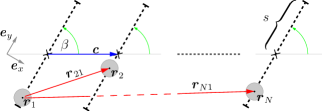
(a)

Figure 1: Geometry of the open linear chain of rowers that move back and forth on line segments (dashed lines) with length $2s$. The line segments are oriented along the $y$ axis, their centers are separated by the lattice vector c, and the tilt angle between the segments and c is $\beta$.

Figure 1 depicts the geometry of the linear chain of rowers separated by the lattice vector c. The chain has open ends for which we present most of our results. The effect of periodic boundary conditions is briefly discussed in Sec. 4.2. While Cosentino Lagomarsino et al. and Kotar et al. let the rowers beat parallel to the lattice vector c lagomarsinoEtAl ; kotarEtAl , we introduce the tilt angle $\beta$ of line segments against the lattice vector c as global parameter. The line segments are oriented along the $y$ axis and their centers are located at $m\textbf{\emph{c}}=mc(\sin\beta,\cos\beta)$. Together with the asymmetry of the power and recovery stroke introduced below, this tilt breaks the left-right symmetry of the linear chain of rowers and metachronal waves can then propagate with a definite direction either to the left or to the right.

The driving forces acting on the rowers are always parallel to the line segments. Furthermore, we only consider the $y$ components of the hydrodynamic-interaction terms in Eq. (1) and neglect their $x$ components. This reduces the spatial degrees of freedom of each rower to one and its position is given by $\textbf{\emph{r}}_{m}=m\textbf{\emph{c}}+y_{m}\textbf{\emph{e}}_{y}$ (Fig. 1). In order to check this approximation, we allowed excursions of the rowers perpendicular to their line segments by introducing strong harmonic potentials along the $x$ direction. In simulations of this two-dimensional rower model, we only found minor quantitative but no qualitative differences to the results presented below in various examples. We therefore decided to work with the one-dimensional model, which needs much less simulation time.

In addition to the continous displacement variable $y_{m}$, we use the discrete “geometric-switch” variable $\sigma_{m}=\pm 1$ to describe the rower’s state. It was first introduced by Gueron and Levit-Gurevich gueronEtAl . It determines the direction of the driving force and hence if the rower moves parallel to $\textbf{\emph{e}}_{y}$ ($\sigma_{m}=1$) or antiparallel to $\textbf{\emph{e}}_{y}$ ($\sigma_{m}=-1$). The geometric switch changes sign when the rower reaches the displacement $s$ from the center of the line segment. Therefore, the rower performs a periodic motion and can be regarded as a driven oscillator. For a driving force with constant magnitude $F_{0}$ and non-interacting rowers, the period of this oscillation is $\tau=4s/(\mu_{0}F_{0})$. In several figures presented below we will refer time $t$ to the period $\tau$. For later use we assign to each rower a phase variable that grows by $2\pi$ during one cycle starting from the center of the line segment ($y_{m}=0$):

$$\varphi_{m}\!=2\pi n_{m}+\frac{\pi}{2}\sigma_{m}y_{m}+\begin{cases}0&\text{if }y_{m}\in[\;\;0,\;\;1)\,\wedge\,\sigma_{m}\!=\;\>1\\ \pi&\text{if }y_{m}\in[\;\;1,-1)\,\wedge\,\sigma_{m}\!=\!-\!1\\ 2\pi&\text{if }y_{m}\in[-1,\;\>0)\,\wedge\,\sigma_{m}\!=\;\>1\end{cases}$$ (3)

Here, $n_{m}\in\mathbb{N}$ is increased by one after each completion of a cycle.

We define the reduced driving force on the $m$-th rower, $F_{m}(y_{m},\sigma_{m})=-\partial V(y_{m},\sigma_{m})/\partial y_{m}$, using the reduced potential

$$V(y_{m},\sigma_{m})=\left(-\sigma_{m}y_{m}+\frac{\epsilon y_{m}^{2}}{2}\right)(\alpha\sigma_{m}+1)+V_{P}\,.$$ (4)

The linear term on the right-hand side gives a constant force with magnitude $F_{0}$ and the second term contributes a harmonic part to the potential with curvature $\epsilon\!\in\!(-1,1)$. The asymmetry parameter $\alpha\!\in\!(-1,1)$ distinguishes between a fast power and a slow recovery stroke. Curvature $\epsilon$ and asymmetry $\alpha$ are the two important parameters of the potential. Finally, we also introduce a harmonic potential $V_{P}$ centered at the switching points ($y_{m}=\pm 1$). It acts only when the rower passes the switching point due to hydrodynamic drag forces from neighboring rowers and, thereby, prevents the rower to trespass the switching point significantly. In Fig. 2 we illustrate the reduced potential for $\alpha=0.2$ and for two curvature values, $\epsilon=0$ and $-0.7$. The geometric switch variable is represented by solid ($\sigma=1$) and dashed ($\sigma=-1$) lines, respectively. With the choice of a positive $\alpha=0.2$, the fast power stroke is performed at $\sigma=1$ when the rower moves in positive $y$ direction.

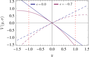
(a)

Figure 2: Potential of the driving force for $\epsilon=0$ and $\epsilon=-0.7$ and $\alpha=0.2$. The solid lines belong to $\sigma=1$ and the dashed lines to $\sigma=-1$. For positive $\alpha$ the fast power stroke is performed from left to right.

Note that Cosentino Lagomarsino et al. lagomarsinoEtAl define the power and recovery stroke by introducing different Stokes mobilities in the forward ($\sigma=1$) and backward ($\sigma=-1$) motion. Such a choice does not directly affect the hydrodynamic-interaction terms in Eq. (1) since the driving forces are the same. We tested that this method does not effectively break the left-right symmetry of the rower chain in order to create metachronal waves which run in one direction along the whole chain. In contrast, by altering the strength of the driving force we are able to break the directional symmetry of the chain and induce metachronal waves with a definite direction.

A single rower performs now the following oscillatory motion in a potential with negative curvature as illustrated in Fig. 2. It starts off slowly from a switching point (e.g. at $y_{m}=-1$) and increases its velocity until it reaches the opposing switching point (e.g. at $y_{m}=1$). Here the switch variable $\sigma$ changes sign and the rower is dragged back into the opposite direction. Both, direction and magnitude of the velocity change discontinuously at the switching points. The non-zero curvature $\epsilon$ of the potential increases the period of a single rower relative to $\tau$, the period when only a constant force $F_{0}$ acts.

3 Synchronization of two rowers

Figure 3 summarizes our numerical studies on the dynamics of two rowers. The time evolution of the relative phase $\Delta\varphi=\varphi_{2}-\varphi_{1}$ crucially depends on the curvature $\epsilon$ of the driving-force potential. While positive $\epsilon$ leads to antiphase synchronization regardless of the initial phase difference, the rowers assume the same phase when $\epsilon$ is negative. For a constant force ($\epsilon=0$), $\Delta\varphi$ keeps its initial value and does not change in time. We now develop an understanding for this behavior.

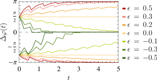
(a)

Figure 3: The synchronization of two rowers depends on the curvature $\epsilon$ of the driving-force potential. The time evolution of the relative phase $\Delta\varphi=\varphi_{2}-\varphi_{1}$ is shown for two intitial values, $\Delta\varphi=\pi/2$ and $-3\pi/4$. Power and recovery stroke are symmetric, i.e. $\alpha=0$, the tilt angle $\beta=\pi/4$, and the distance of the rowers is $c=0.28$.

For zero curvature $\epsilon$ of potential $V$ and identical power and recovery stroke, $\alpha=0$, the driving force on both particles is constant and identical throughout one beating cycle. Then the mutual hydrodynamic interactions are always equal in absolute value and thus the phase difference between both rowers does not change. The latter is even valid for the phase difference after one beating cycle if $\alpha\neq 0$. Due to the different forces in the power and recovery stroke, particles change their relative phase when they move in opposite direction. However, during one beating cycle each particle performs both the power and the recovery stroke. So, after one period the phase difference assumes its initial value and synchronization does not occur. We stress again that $\alpha$ is significant only for breaking the left-right symmetry in a chain of rowers in conjunction with the tilt angle $\beta$ which then enables metachronal waves that travel in one direction only.

A non-zero curvature in the driving-force potential breaks the symmetry in the hydrodynamic interactions between two rowers and leads to synchronization as already demonstrated in Fig. 3. Whilst Cosentino Lagomarsino et al. restrict $\epsilon$ to be positive, which leads to an antiphase synchronization lagomarsinoEtAl ; kotarEtAl , we also allow negative values, thereby obtaining the desired in-phase synchronization. The significant part of the synchronization is accomplished when both rowers move in opposite directions. We first consider the case $\epsilon<0$ and assume that the preceding rower has just reached its switching point. After activating the geometrical switch, the preceding rower experiences a weaker driving force than the succeeding rower before the switching point (see Fig. 2). Therefore, the flow field initiated by the succeeding rower is stronger and slows down the preceding rower more strongly than vice versa. This leads to a decrease of the phase difference $\Delta\varphi$ until the succeeding rower also reaches the switching point. Then both rowers move in the same direction and the phase difference $\Delta\varphi$ increases again. However, in total a decrease is realized during one cycle as illustrated in Fig. 3. For positive $\epsilon$, the preceding rower slows down the succeeding rower more strongly and $\Delta\varphi$ increases on average during one cycle until it reaches the value $\pi$. To conclude, in the time evolution of the phase difference $\Delta\varphi=0$ is a stable and $\Delta\varphi=\pm\pi$ is an unstable fixpoint for $\epsilon<0$, whereas for positive $\epsilon$ the stability of the fixpoints is reversed.

In a very attractive experimental realization of the two-particle system, Kotar et al. use optical traps to create the driving-force potential with positive curvature $\epsilon>0$ kotarEtAl . Each colloidal bead is confined in the harmonic regime of the potential well created by a laser beam. The potential well switches between two positions such that a bead is always driven towards the potential minimum. The “geometric switch” is then initiated before the bead reaches the minimum. In agreement with our results, the two beads synchronize in antiphase. The trap potential created by an optical tweezer has a regime further away from the minimum, where the curvature is negative opticaltweezers . We propose to use this regime to realize in-phase synchronization experimentally.

4 Synchronization in a chain of rowers

4.1 Complex order parameter

The collective dynamics of a chain of several hundred rowers strongly depends on the parameters introduced above that determine the driving-force potential and the geometry of the rower chain. In order to classify the collective dynamics and, in particular, to identify metachronal waves, we introduce a complex order parameter and study its longterm behavior.

For an array of $N$ oscillators, we can introduce $N-1$ phase differences $\{\Delta\varphi_{1},\dots,\Delta\varphi_{N-1}\}$ and their phasors $z_{n}=e^{i\Delta\varphi_{n}}\in\mathbb{C}$, where $\Delta\varphi_{n}=\varphi_{n+1}-\varphi_{n}$. We define our complex order parameter as the mean of the phasors,

$$Z=Ae^{i\varPhi}:=\frac{1}{N-1}\sum\limits_{n=1}^{N-1}z_{n}=\frac{1}{N-1}\sum\limits_{n=1}^{N-1}e^{i\Delta\varphi_{n}}\enspace.$$ (5)

The magnitude $A$ and polar angle $\varPhi$ lie in the respective ranges $A\in[0,1]$ and $\varPhi\in[-\pi,\pi)$. We add a note here. In order to determine if oscillators fully synchronize to equal phases, usually the order paramter averages over the phasors $e^{i\varphi_{n}}$ for phases $\varphi_{n}$ syncr_Definitions ; syncrRosenblumEtAl . However, this definition is not appropriate for identifying metachronal waves.

For a large number $N$ of rowers with random phases, the phasors $z_{n}$ are uniformly distributed over the unit circle in the complex plane. Their mean, the complex order parameter $Z$, is close to 0, i.e., $A\approx 0$ with arbitrary $\varPhi$. If, on the other hand, the system displays a stable metachronism, where pairs of neighboring oscillators are phase locked with the same phase difference syncr_Definitions , then $z_{n}=z_{m}$ for all phasors $m,n\in\{1,\dots,N-1\}$. In this case, $Z$ is stationary. It lies on the unit circle in the complex plane ($A=1$) and $\varPhi$ is equal to the phase difference of each pair of oscillators.

In the following, we will also observe states where the long-time limit of $Z$ fluctuates around a constant value. We therefore introduce the average values

$$\bar{A}=\frac{1}{\Delta t}\int_{T-\Delta t}^{T}A(t)dt\qquad\bar{\varPhi}=\frac{1}{\Delta t}\int_{T-\Delta t}^{T}\varPhi(t)dt\enspace,$$ (6)

where $T$ is the final time of the simulation run and $\Delta t$ an appropriately chosen time interval. In addition, we also quantify fluctuations of the order parameter by calculating the standard deviations $\sigma_{A}$ and $\sigma_{\varPhi}$ of the time averaged values.

4.2 Synchronization in an unbounded fluid

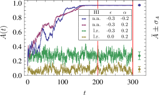
(a)

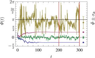
(b)

Figure 4: Absolute value (a) and polar angle (b) of the order parameter $Z(t)$ as a function of time for a chain of 200 rowers for different parameter sets. The global parameters are $c=0.28$ and $\beta=\pi/4$ and for all graphs the rowers start with the same random distribution of phases. The vertical red lines ($\centerdot\!\!\centerdot\!\!\centerdot\!\!\centerdot\!\!\centerdot\!\!\centerdot\!\!\centerdot$) mark the time intervall $\Delta t=100$ for which we calculate the time averages $\bar{A}$ and $\bar{\varPhi}$. They are shown as dots on the right-hand side of the corresponding diagrams together with errorbars indicating the respective standard deviations $\sigma_{A}$ and $\sigma_{\varPhi}$. Golden line ($\centerdot\!\!\centerdot\!\!\centerdot\!\!\centerdot\!\!\centerdot\!\!\centerdot\!\!\centerdot$): $\alpha=0.2$ , $\epsilon=0$, and long-range hydrodynamic interactions (l.r. HI) are used. Note for this parameter set we have added $2\pi$ to all negative values of $\varPhi(t)$ to better represent its time dependence. Green line ($\centerdot\!\!\centerdot\!\!\centerdot\!\!\centerdot\!\!\centerdot\!\!\centerdot\!\!\centerdot$): $\alpha=0.2$ and $\epsilon=-0.3$ with l.r. HI. Magenta line ($\centerdot\!\!\centerdot\!\!\centerdot\!\!\centerdot\!\!\centerdot\!\!\centerdot\!\!\centerdot$): $\alpha=0.2$ and $\epsilon=-0.3$ but hydrodynamic interactions are artificially restricted to nearest neighbors (n.n. HI). A metachronal wave occurs that travels in a definite direction. Blue line ($\centerdot\!\!\centerdot\!\!\centerdot\!\!\centerdot\!\!\centerdot\!\!\centerdot\!\!\centerdot$): same situation but $\alpha=-0.2$. The mean phase $\bar{\varPhi}$ is reversed and the metachronal wave travels in the opposite direction.

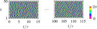
(a)

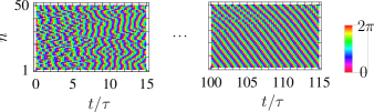
(b)

Figure 5: Color coded phases of the the first 50 rowers in a chain of 200 rowers as a function of time $t$. The global parameters are $\alpha=0.2$, $c=0.28$, and $\beta=\pi/4$. The simulations start with $\epsilon=0$ and at $t=5$ the curvature changes to $\epsilon=-0.3$ in order to visualize the onset of synchronization. (a) For long-range hydrodynamic interactions transient in-phase synchronization occurs locally. (b) For nearest-neighbor interactions metachronal waves are visible.

In Figs. 4(a) and 4(b) we illustrate the temporal evolution of the order parameter $Z(t)$ for an open chain of 200 rowers in different situations. For $\epsilon=0$ and $\alpha=0.2$ [golden graph ($\centerdot\!\!\centerdot\!\!\centerdot\!\!\centerdot\!\!\centerdot\!\!\centerdot\!\!\centerdot$)], magnitude $A(t)$ and, in particular, $\varPhi(t)$ strongly fluctuate in time. Their respective mean values are $\bar{A}\ll 1$ and $\bar{\varPhi}\approx\pi$. Apart from a tendency of neighboring rowers to beat in antiphase, a noticable structure formation does not occur.

We now introduce a negative curvature $\epsilon=-0.3$ in the driving-force potential. The green graphs ($\centerdot\!\!\centerdot\!\!\centerdot\!\!\centerdot\!\!\centerdot\!\!\centerdot\!\!\centerdot$) in Figs. 4(a) and 4(b) still show a strongly fluctuating order parameter. In contrast to $\epsilon=0$ though, we observe a significant increase of the time-averaged magnitude $\bar{A}$. Together with $\bar{\varPhi}\approx 0$ this indicates that some of the rowers synchronize in phase. A further understanding is achieved from Fig. 5(a), where we plot the color-coded phases over time for the first 50 rowers. At $t=0$ we start with curvature $\epsilon=0$ and switch to $\epsilon=-0.3$ at $t=5$. Then chain segments of approximately 8 rowers appear that are fully synchronized in phase as expected for negative curvature. However, after some time these clusters break apart and form somewhere else. The synchronization is only transient since the rowers in the center of a cluster have reduced friction coefficients compared to rowers at the edges due to long-range hydrodynamic interactions. Hence, rowers in the center move faster and destabilize the cluster.

The reported instability is caused by the long-range nature of hydrodynamic interactions. Following Ref. niedermayerEtAl , we artificially make them short-ranged by including only the nearest neighbors in the sum of the dynamic equations (1). The range of hydrodynamic interactions can be controlled close to a surface, as we demonstrate in the next section. Now metachronal waves appear that travel from one end of the chain to the other with a wavelength of approximately eight rowers. Fig. 5(b) demonstrates impressively how the initially uncorrelated rowers evolve into a metachronal wave due to phase-locking. The process is completed for the whole chain after $t=175$. This is also visible in Fig. 4(a) [magenta line ($\centerdot\!\!\centerdot\!\!\centerdot\!\!\centerdot\!\!\centerdot\!\!\centerdot\!\!\centerdot$)] when $A(t)\approx 1$ is achieved. The phase difference [Fig. 4(b)] converges to approximately $\bar{\varPhi}\approx\pi/4$ which gives the corresponding wavelength of 8 rower distances. The very small standard deviations of $\bar{A}$ and $\bar{\varPhi}$ are a further measure that a metachronal wave has been formed nearly perfectly. Finally, reversing the sign of $\alpha$ [blue curves ($\centerdot\!\!\centerdot\!\!\centerdot\!\!\centerdot\!\!\centerdot\!\!\centerdot\!\!\centerdot$) in Figs. 4(a) and 4(b)], which means exchanging the fast power and slow recovery strokes, also reverses the sign of $\bar{\varPhi}$ and the metachronal wave travels in the opposite direction.

To break the left-right symmetry of the rower chain, parameter values $\alpha\neq 0$ and $\beta\neq\pi/2$ are needed but also the distance $c$ of the rowers has to be sufficiently small for creating metachronal waves travelling in one direction. For $\alpha=0$ or $\beta=\pi/2$ or by simply choosing $c>1$, we observe metachronal waves running from the center of the chain into both directions. This is reminiscent to studies of Niedermayer et al. niedermayerEtAl , where beads move on circular trajectories.

Positive curvature $\epsilon>0$ of the driving-force potential reproduces the results of Cosentino Lagomarsino et al. lagomarsinoEtAl . The tendency of neighboring rowers to synchronize in antiphase leads to a metachronism with shorter wavelengths of approximatly 4 rowers. Compared to the case with $\epsilon=-0.3$, the system needs about ten times longer to reach the stationary state.

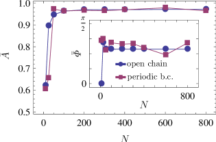
(a)

Figure 6: Averaged magnitude $\bar{A}$ and polar angle $\bar{\varPhi}$ (inset) of the order parameter as a function of the number $N$ of rowers in open (circles) and closed (squares) chains.

We shortly discuss how the chain length of open chains and also periodic boundary conditions influence the occurence of metachronal waves. We concentrate on the same parameters as before ($\epsilon=-0.3$, $\beta=\pi/4$, and $\alpha=\pm 0.2$) and use hydrodynamic interactions restricted to nearest neighbors. This allows us to realize the periodic boundary conditions by a closed chain where the first and last rower interact with each other. Figure 6 compares $\bar{A}$ and $\bar{\varPhi}$ (inset) for open (circles) and closed (squares) chains for different chain lengths. For chain lengths above 50 rowers open and closed chains develop metachronal waves with nearly the same $\bar{A}$ and $\bar{\varPhi}$. So finite size effects become negligible. At shorter chain lengths the dynamics of open and closed chains differ strongly. Whereas for $N=10$ (first data point) the same magnitude $\bar{A}\approx 0.6$ indicates some order but certainly no metachronism, the polar angles reveal different behavior in the two cases. For open chains $\bar{\varPhi}=0$, which means that central rowers synchronize in phase whereas the outer rowers lag behind due to the larger friction they experience. On the other hand, in closed chains, where all rowers have an identical environment, a non-zero mean polar angle $\bar{\varPhi}$ is observed. A closer inspection of the individual rower phases shows that pairs of rowers almost fully synchronize in phase whereas they leave a larger phase gap to the next pair. We discuss these points so detailed here because in an experimental realization finite size effects of the chain may become important.

4.3 Synchronization near an infinitely extended wall

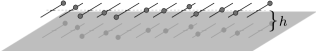
(a)

Figure 7: A chain of rowers a distance $h$ above an infinitely extended wall.

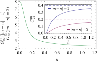
(a)

Figure 8: Inset: The relevant component $G_{22}^{\text{Bl}}$ of the Blake tensor as a function of $h$ for, both, nearest-neighbor ($|m-n|=1$) and next-nearest neighbor ($|m-n|=2$) rowers. The distance of the nearest-neighbor and next-nearest neighbor rowers are $c=0.28$ and $2c=0.56$, respectively. The dashed lines indicate the respective values of the Oseen tensor, i.e., for height $h\rightarrow\infty$. Large graph: ratio of both components, $G_{22}^{\text{Bl}}(|m-n|=1)/G_{22}^{\text{Bl}}(|m-n|=2)$.

So far we artificially restricted hydrodynamic interactions to nearest neighbors in order to make them short-ranged. In reality, the range of hydrodynamic interactions can be tuned by placing the chain of rowers a distance $h$ above an infinitely extended wall. As sketched in Fig. 7, the rowers beat parallel to this wall. In order to describe the cross mobilities of point particles close to a wall, the Oseen tensor has to be replaced by the Blake tensor blake_singularities_1974_etAl . The latter converges to the Oseen tensor for $h\rightarrow\infty$. So, by continuously changing the height $h$, one can control the range and strength of hydrodynamic interactions. They decay with $1/r$ at large distances $h$ from the wall, thus being of long range. In the vicinity of the wall, they decay with $1/r^{3}$ and justify the approximation of nearest-neighbor interactions used in Ref. niedermayerEtAl . In Fig. 8 in the inset we plot the relevant component $G_{22}^{\text{Bl}}$ of the Blake tensor as a function of $h$ for, both, nearest-neighbor and next-nearest-neighbor rowers. The dashed lines indicate the respective values of the Oseen tensor that are reached in the limit $h\rightarrow\infty$. On the other hand, for $h\rightarrow 0$ the relative strength of the nearest-neighbor component $G_{22}^{\text{Bl}}$ compared to the next-nearest-neighbor component increases as the large graph in Fig. 8 demonstrates. So, we expect to observe with decreasing $h$ a transition from transient synchronization to the formation of metachronal waves.

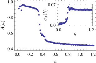
(a)

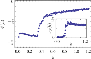
(b)

Figure 9: Average magnitude (a) and polar angle (b) of the order parameter $Z$ for a rower chain situated at a height $h$ above a bounding wall. The insets show the respective standard deviations. The global parameters of the open chain with $N=200$ rowers are $\beta=\pi/4$, $c=0.28$, $\alpha=-0.2$, and $\epsilon=-0.4$. For $h>0.15$, the total simulation time was $T=3750$ and the time window for determining the averages was chosen sufficiently large, $\Delta t=2500$, in order to minimize fluctuations of $\bar{A}$ and $\bar{\varPhi}$. For $h\leq 0.15$, the simulation time was extended to $T=6250$ to ensure that a stationary metachronal state was reached and $\Delta t=125$.

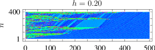
(a)

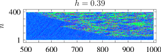
(b)

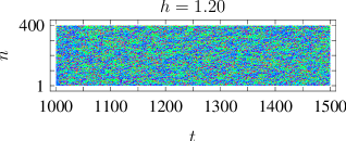
(c)

(d)

Figure 10: Color-coded phase differences of neighboring rowers as a function of time in a chain of 400 rowers. The simulation starts at a height of $h=0.20$, which is then increased to $h=0.39$ and $h=1.20$ at times $t=500$ and $t=1000$, respectively. At $h=0.20$ a metachonal wave develops and finally stretches over the entire chain. At $h=0.39$ the metachronism starts to break apart and transient synchronization with larger patches of correlated rowers are visible. At $h=1.20$ the patches become smaller.

This is demonstrated in Figs. 9(a) and 9(b), where we plot the time-averaged magnitude $\bar{A}$ and polar angle $\bar{\varPhi}$ of the order parameter $Z$ as a function of the height $h$. The insets depict the corresponding standard deviations. At hights $h$ smaller than 0.35, $\bar{A}>0.9$ clearly indicates metachronism with an absolute phase difference between rowers smaller than $\pi/4$. It only varies slightly with $h$ so that the wavelengths of the metachronal waves correspond to 9 to 10 rowers. Also the very small standard deviations are typical for metachronism. Then a relatively sharp transition occurs at $h=0.35$ into a state of transient synchronization. The amplitude $\bar{A}$ decreases by a factor of two and the negative $\bar{\varPhi}$ grows towards zero. In particular, the destruction of metachronism is indicated by a strong increase in the standard deviations showing that amplitude $A$ and polar angle $\varPhi$ of the order parameter fluctuate strongly. In Fig. 10 the transition is also visible. We show the color-coded phase differences between neighboring rowers as a function of time. At $t=0$ we start at a hight $h=0.20$ and then during the simulation switch to $h=0.39$ at $t=500$ and to $h=1.20$ at $t=1000$. Whereas the nearly uniform blue region at $h=0.20$ shows the existence of metachronal waves, they dissolve with time at $h=0.39$ and transient patches of same color indicate some synchronization. At $h=1.20$ the patches become smaller corresponding to a further decrease in $\bar{A}$ and the results are similar to our findings in the unbounded fluid [compare green graphs in Figs. 4(a) and 4(b)].

Our results show that metachronal waves in a chain of in-phase synchronizing rowers can only develop in the vicinity of a surface, where the range of hydrodynamic interactions is strongly reduced. Long-range hydrodynamic interactions destabilize the waves since they lead to the formation of transient clusters synchronized in-phase.

5 Conclusions

In order to shed light on the essential features for obtaining metachronal waves, we implemented a chain of oscillators or rowers that are driven by an external non-linear force derived from a driving-force potential. Two rowers synchronize in antiphase when the curvature of the force potential is positive or in phase when the curvature is negative. We concentrated on the latter case and introduced a suitable order parameter for identifying metachronal waves. Our investigations show that metachronal waves exist only when the range of hydrodynamic interactions is restricted either artificially or by the presence of a bounding surface as in any relevant biological system. The negative curvature in the driving force potential leads to metachronal waves with wavelengths of 7-10 rower distances. Curiously, in paramecium a wavelength including eight cilias is observevd machemerParamecium . In comparison, positive curvature that promotes antiphase synchronization in a rower pair only gives shorter wavelengths of around four rowers lagomarsinoEtAl . In order to obtain waves that travel either in one or the other direction along the chain, we break its left-right symmetry by tilting the rower segment with respect to the normal of the chain and distinguish between a fast power and slow recovery stroke. These measures are only effective when the rowers are sufficiently close to each other ($c<1$).

Metachronal waves and their defining properties, such as the wavelength and the propagational direction relative to the direction of the power stroke, are an essentially two-dimensional phenomenon as Machemer pointed out machemerParamecium . Therefore, it will be important to extend current research towards models defined on two-dimensional lattices. This should give further insight into the fascinating properties of metachronal waves. Theoretical work in this direction was carried out on microfluidic rotors Grzybowski:2000 ; Lenz:2003 ; golestanian2010EtAl . However, amongst the great variety of beautiful patterns evolving, in particular, in Ref. golestanian2010EtAl , metachronal waves as seen on ciliated surfaces cannot be observed. We have recently started to look at two-dimensional regular arrays of mainly stiff rods attached to a surface. We let them perform strokes where they move on a cone tilted with respect to the normal of the surface Downton10 . When we divide the beating cycle into a fast power and a slow recovery stroke, the latter acting when the rod is close to the surface, metachronal waves emerge. For a planar stroke see Ref. Elgeti06 . We will continue working on our system and also think about closed curved surfaces where topological constraints arise.

Appendix A Mobilities for a fluid bounded by a plane wall

When the fluid is bounded by an infinitely extended wall in the $xy$ plane, the mobilities for point-like particles assume the following expressions. The self-mobility depends on the distance $h$ from the bounding wall DufresneEtAl :

$$\textbf{\emph{M}}_{mm}(\textbf{\emph{r}}_{m})=\mu_{0}\left[\mathbbm{1}-\frac{9}{16}\frac{a}{h}\begin{pmatrix}1&0&0\\ 0&1&0\\ 0&0&2\\ \end{pmatrix}\right]\,,$$ (7)

and the Blake tensor $\textbf{\emph{G}}^{\text{Bl}}(\textbf{\emph{r}})$ provides the cross mobilities

$$\textbf{\emph{M}}_{mn}(\textbf{\emph{r}}_{m},\textbf{\emph{r}}_{n}) = \textbf{\emph{G}}^{\text{Bl}}(\textbf{\emph{r}}_{m},\textbf{\emph{r}}_{n})$$

$$= \textbf{\emph{G}}^{\text{Os}}(\textbf{\emph{r}}_{m}-\textbf{\emph{r}}_{n})-\textbf{\emph{G}}^{\text{Os}}(\textbf{\emph{r}}_{m}-\bar{\textbf{\emph{r}}}_{n})$$

$$+2h^{2}\textbf{\emph{G}}^{\text{So}}(\textbf{\emph{r}}_{m}-\bar{\textbf{\emph{r}}}_{n})-2h\textbf{\emph{G}}^{\text{St}}(\textbf{\emph{r}}_{m}-\bar{\textbf{\emph{r}}}_{n})\,,$$

where $\textbf{\emph{r}}_{n}=(x_{n},y_{n},h)$ is the location of the point force and $\bar{\textbf{\emph{r}}}_{n}=(x_{n},y_{n},-h)$ is its image point vilfanEtAl ; blake_singularities_1974_etAl . Using the Kronecker symbol $\delta_{\lambda\nu}$, the components of the so-called source doublet $\textbf{\emph{G}}^{\text{So}}$ and Stokes doublet $\textbf{\emph{G}}^{\text{St}}$ read, respectively,

$$G_{\lambda\nu}^{\text{So}}(\textbf{\emph{x}}) =\frac{1}{8\pi\eta}(1-2\delta_{\nu 3})\frac{\partial}{\partial x_{\nu}}\left(\frac{x_{\lambda}}{\lvert\textbf{\emph{x}}\rvert^{3}}\right)$$ (9)

$$G_{\lambda\nu}^{\text{St}}(\textbf{\emph{x}}) =(1-2\delta_{\nu 3})\frac{\partial}{\partial x_{\nu}}G_{\lambda 3}^{\text{Os}}(\textbf{\emph{x}})\,.$$ (10)

References

- (1) D. Bray, Cell Movements: From Molecules to Motiliy, 2nd ed., (Garland Publishing, New York, 2001).
- (2) E. M. Purcell, Am. J. Phys. 45, 3 (1977).
- (3) E. Lauga and T. R. Powers, Rep. Prog. Phys. 72, 096601 (2009).
- (4) M. T. Downton and H. Stark, J. Phys.: Condens. Matter 21, 204101 (2009).
- (5) H. Machemer, J. Exp. Biol. 57, 239 (1972).
- (6) R. W. Linck, Cilia and Flagella in Encyclopedia of Life Sciences (Wiley, Chichester, 2001), www.els.net.
- (7) C. Brennen and H. Winet, Ann. Rev. Fluid Mech. 9, 339 (1977).
- (8) M. Cosentino Lagomarsino, P. Jona, B. Bassetti, Phys. Rev. E 68, 21908 (2003).
- (9) A. Vilfan and F. Jülicher, Phys. Rev. Lett.96, 058102 (2006).
- (10) P. Lenz and A. Ryskin, Phys. Biol. 3, 285-294 (2006).
- (11) T. Niedermayer, B. Eckhardt, and P. Lenz, Chaos 18, 37128 (2008).
- (12) J. Kotar, M. Leoni, B. Bassetti, M. Cosentino Lagomarsino, and P. Cicuta, PNAS 107, 7669 (2010).
- (13) S. Gueron, K. Levit-Gurevich, N. Liron, and J. J. Blum, PNAS 94, 6001 (1997).
- (14) S. Gueron and K. Levit-Gurevich, PNAS 96, 12240 (1999).
- (15) B. Guirao and J. F. Joanny, Biophys. J. 92, 1900 (2007).
- (16) E. M. Gauger, M T. Downton, and H. Stark, Eur. Phys. J. E 28, 231 (2009).
- (17) J. Blake, J. Theor. Biol. 52, 67 (1975).
- (18) M. Sleigh, J. Exp. Biol. 37, 1 (1960).
- (19) S. L. Tamm, J. Exp. Biol. 113, 401 (1984).
- (20) I. Gibbons, J. Biophys. Biochem. Cytol. 11, 179 (1961).
- (21) P. Satir and M. A. Sleigh, Annu. Rev. Physiol. 52, 137 (1990).
- (22) M. A. Chilvers, A. Rutman, and C. O’Callaghan, J. Allergy Clin. Immunol. 112, 518 (2003).
- (23) Y. Kuramoto, Chemical Oscillations, Waves, and Turbulence (Springer, Berlin, 1984).
- (24) Y.T. Yang, C. Callegari, X.L. Feng, K.L. Ekinci and M.L. Roukes, Nano Letters 6, 583 (2006).
- (25) D. Rugar, R. Budakian, H. J. Mamin, and B. W. Chui, Nature 430, 329 (2004).
- (26) A. N. Cleland and M. L. Roukes, Nature 392, 160 (1998).
- (27) I. H. Riedel-Kruse, A. Hilfinger, J. Howard and F. Julicher, HFSP J. 1, 192 (2007).
- (28) J. A. Acebrón, L. L. Bonilla, C. J. Pérez Vicente, F. Ritort, and R. Spigler, Rev. Mod. Phys. 77, 137 (2005).
- (29) A. Pikovsky, M. Rosenblum and J. Kurths, in Analysis and Control of Complex Nonlinear Processes in Physics, Chemistry and Biology , edited by L Schimansky-Geier, B. Fiedler, J. Kurths and E. Schöll (World Scientific, Singapore, 2007).
- (30) M. Kim and T. R. Powers, Phys. Rev. E 69, 061910 (2004).
- (31) M. Reichert and H. Stark, Eur. Phys. J. E 17, 493 (2005).
- (32) B. Qian, H. Jiang, D. A. Gagnon, K. S. Breuer and T. R. Powers, Phys. Rev. E 80, 61919 (2009).
- (33) B. A. Grzybowski, H. Stone, G. M. Whitesides, Nature 405, 1033 (2000).
- (34) P. Lenz, J.-F. Joanny, F. Jülicher, and J. Prost, Phys. Rev. Lett. 91, 108104 (2003).
- (35) N. Uchida and R. Golestanian, Phys. Rev. Lett. 104, 178103 (2010).
- (36) R. E. Goldstein, M. Polin, and I. Tuval, Phys. Rev. Lett. 103, 168103 (2009).
- (37) G. Taylor, Proc. R. Soc. A 209, 447 (1951).
- (38) Y. Yang, J. Elgeti, and G. Gompper, Phys. Rev. E 78, 061903 (2008).
- (39) G. J. Elfring and E. Lauga, Phys. Rev. Lett. 103, 088101 (2009).
- (40) G. J. Elfring, O. S. Pak, E. Lauga, J. Fluid Mech. 646, 505 (2010).
- (41) J. Blake and A. Chwang, J. Eng. Math. 8, 23 (1974)
- (42) D. G. Grier, Nature 424, 810 (2003)
- (43) E. R. Dufresne, T. M. Squires, M. P. Brenner and D. G. Grier, Phys. Rev. Lett. 85, 3317 (2000).
- (44) M. Downton and H. Stark, unpublished results.
- (45) J. Elgeti, Sperm and Cilia Dynamics, Ph.D. Thesis, Universität zu Köln (2006).