Universal patterns in sound amplitudes of songs and music genres

Abstract

We report a statistical analysis over more than eight thousand songs. Specifically, we investigate the probability distribution of the normalized sound amplitudes. Our findings seems to suggest a universal form of distribution which presents a good agreement with a one-parameter stretched Gaussian. We also argue that this parameter can give information on music complexity, and consequently it goes towards classifying songs as well as music genres. Additionally, we present statistical evidences that correlation aspects of the songs are directly related with the non-Gaussian nature of their sound amplitude distributions.

In recent years, studies of complex systems have become widespread among the scientific community, specially in the statistical physics oneAuyang ; Jensen ; Barabasi ; Boccara ; Sornette . Many of these investigations deal with data records ordered in time or space (i.e., time series), trying to extract some features, patterns or laws that may be present in the systems studied. This approach has been successfully applied to a variety of fields, from physics and astronomyChandrasekhar to geneticsPeng and economyMantegna . Moreover, this framework has been a trend towards investigating and modeling interdisciplinary fields, such as religionPicoli , electionsFortunato , vehicular trafficChowdhury , tournamentsRibeiro , and many others. These few examples and social phenomena in general Castellano illustrate as physicists have gone far from their traditional domain of investigations.

Music is a well known worldwide social phenomenon linked to the human cognitive habits, modes of consciousness as well as historical developmentsDeNora . In the direction of music’s social role, some authors investigated collective listening habits. For instance, Lambiotte and AusloosLambiotte analyzed data from people music library finding audience groups with the size distribution following a power law. They also investigated correlations among these music groups, reporting non-trivial relationsLambiotte2 . In another work, Silva et al.Silva studied the network structure of the song writers and the singers of Brazilian popular music (mpb). There is also an interest in the behavior of music salesLambiotte3 as well as in the success of musiciansDavies ; Borges ; Hu .

Despite these cultural aspects, songs form a highly organized system presenting very complex structures and long-range correlations. All these features have attracted the attention of statistical physicists. In a seminal paper, Voss and ClarkeVoss analyzed the power spectrum of radio stations and observed a $1/f$ noise like pattern. They also showed that the correlation can extend to longer or shorter time scales, depending on the music genre. Hsü and HsüHsu investigated the changes of acoustic frequency in Bach’s and Mozart’s compositions, finding self-similarity and fractals structures. In contrast, they report no resemblance to fractal geometryHsu2 for modern music. Fractal structures have also been reported in the study of sequences of music notesSu , where Su and WuSu2 suggest that the multifractal spectrum can be used to distinguish different styles of music. By using sound amplitudes of songs, Bigerelle and IostBigerelle achieved a classification based on fractal dimension using the entire frequency range. However, as raised by Ro and KwonRo , the $1/f$ analysis in the region below 20 Hz might not classify music genres. Gündüz and GündüzGunduz reported analysis of several Turkish songs by using many techniques. Beltrán del Río et al.Rio evaluated the rank distribution of music notes of a large selection finding a good agreement with a two parameter beta distribution. Dagdug et al.Dagdug investigated a specific piece of Mozart employing detrended fluctuation analysis (DFA)Peng2 . Applying DFA in a volatility-like series, Jennings et al.Jennings found quantitative differences in the Hurst exponent depending on the music genre.

Figure 1: The normalized sound amplitude of (a) a classical piece and (b) a heavy metal song (labeled in the figure). Note that the signals are quite different, the first one presents a more complex structure characterized by “bursts” while the second resembles a Gaussian noise.

In this brief literature review, we see that special attention was paid to the fractal structures of music, correlations and power spectrum analysis. However, much less attention has been paid to the understanding of the amplitude distribution. This last point has been noted by Diodati and PiazzaDiodati . In their work, they investigated the distribution of times and sound amplitudes larger than a fixed value. By using this kind of return interval analysisSanthanam , they found Gaussian distributions in the amplitude for jazz, pop, and rock music, while non-Gaussians emerge for classical pieces. Here, we directly investigate the amplitude distributions of songs of several genres without employing a threshold value as considered by Diodati and Piazza. Moreover, our analysis goes towards finding patterns in the amplitude sound distribution by using a suitable one-parameter probability distribution function (pdf). In the following, we present the dataset used in our investigation, the analysis of the shape of the resulting distributions and our conclusions.

Not all sound is music, but certainly music is made by sounds. The sounds that we hear are consequence of pressure fluctuations traveling in the air and hitting our ears. These audible pressure fluctuations can be converted into a voltage signal $u_{t}$ by using a record system and stored, for instance, in a compact disk (CD). Our analysis is focused on this time series $u_{t}$ that we call sound amplitude. In the case of songs stored in CDs, $u_{t}$ has a standard sampling rate of 44.1 kHz and encompasses the full audible human range (approximately between 20 Hz and 20 kHz).

As database we have 8115 songs of nine different music genres: classical (907), tango (992), jazz (700), hip-hop (876), mpb (580), flamenco (524), pop (998), techno (900) and heavy metal (1638). The songs were chosen so as to cover a large amount of composers/singers. For instance, for classical music, we have taken pieces from Bartók, Beethoven, Berlioz, Brahms, Bruch, Chopin, Dvorak, Fauré, Grieg, Malher, Marcello, Mozart, Rachmaninov, Strauss, Schuber, Schumann, Scriabin, Shostakovich, Sibelius, Stravinsky, Tchaikovsky, Verdi, Vivaldi, and others.

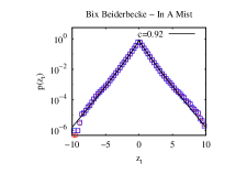
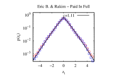
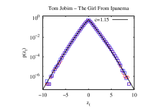
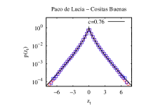
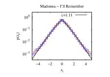
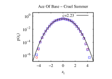
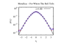
Figure 2: (color online) Histograms of some representative songs (labeled in the figure) in comparison with the stretched Gaussian Eq.(1). The squares (circles) is the right (left) channel of the stereo audio. As we see, the two channels are quite similar in the sense that the statistical results do not dramatically change when considering the right or left channel.

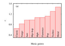
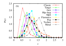
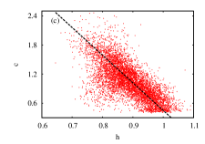
Figure 3: (color online) (a) In ascending order, the mean value of the parameter $c$ corresponding to the stretched Gaussians employed for each music genre considered here. (b) The distribution of the parameter $c$ for each genre. (c) Scatter plot of the parameter $c$ versus the Hurst exponent, $h$, obtained via detrended fluctuation analysis (DFA)Peng3 ; Kantelhardt of sound intensity $z_{t}^{2}$. The dashed line is a guide for our eyes.

When a time series is analyzed, a way to view its variability (complexity) is at least in part by investigating its pdf. In the case of music, the mean amplitude is approximately zero since a vibration essentially occurs around this value. In addition, the mean (global) intensity is not relevant to the variability (complexity) of a song. Motivated by these facts, our research is based on the pdf of recorded data regardless of their mean value and their real amplitudes. In other words, we are considering that the complexity of a song is not related to its mean intensity but with the relative variability of the amplitudes. Thus, instead of employing the amplitude $u_{t}$ in different time instants $t$, we focus attention on $u_{t}$ subtracted from its mean value $\mu$ and divided by its standard deviation $\sigma$. This corresponds to using $z_{t}=(u_{t}-\mu)/\sigma$ instead of $u_{t}$. Figure 1 illustrates the behavior of $z_{t}$ for two songs, a classical piece and a heavy metal song. This figure is enough to reveal qualitative differences between these two songs. In the classical piece, we can observe some kind of bursts giving rise to a non-Gaussian distribution. However, for the heavy metal song, the signal is very similar to a Gaussian noise – no complex structure is perceptible.

Motivated by these distinct behaviors, we investigate the distribution of $z_{t}$ for all the songs in our data set. In Figure 2, we show the pdf for some representative songs. As we can verify from this figure, the shape of distributions goes from a long tail to Laplace to Gaussian distribution. A family of functions that has the Gaussian and the Laplace distributions as particular case is given by the stretched Gaussianrichardson $p(z)=N\exp(-b|z|^{c})$, where $N$ is the normalization constant, $b$ is directly related to the standard deviation and $c$ is a positive parameter. Since the distribution $p(z)$ is normalized to unity and the variable $z$ is defined in such way that its standard deviation is equal to one, the parameters $N$ and $b$ become a function exclusively of $c$, leading to

$$p(z)=\frac{c}{2}\left(\!\frac{\Gamma(3/c)}{\Gamma(1/c)^{3}}\right)^{\!1/2}\!\!~{}\exp\!\left(\!-\left(\frac{\Gamma(3/c)}{\Gamma(1/c)}\right)^{\!c/2}\!|z|^{c}\right),$$ (1)

with $\Gamma[w]$ being the Euler gamma function. Also in Figure 2 the least square fits to the data of the above function are shown. Observe that we find a good agreement between the data and the model for the songs represented in this figure, and a similar agreement have been found for the others (at least in the central part of the distribution).

The only model parameter is $c$ and it may give useful information about music complexity. First note that for values of $c$ smaller than one heavy tail distribution emerge. In some sense, these heavy tails reflect the complex structures that we see in Figure 1a, i.e., larger fluctuations. The increasing of $c$ makes the tails shorter and recover some known distributions (Laplace for $c=1$ and Gaussian for $c=2$). In this context, a shorter tail indicates that larger fluctuations become rare, leading to music signal very similar to a Gaussian noise (see Figure 1b). From the musical point of view, the word complexity may be related to several aspects of the song or even with music taste. In present context, it should be viewed a comparative measurement, i.e., a measure of how the empirical distributions differs from the Gaussian one.

Based on the above discussion, we may use $c$ to sort the songs and music genres in a kind of complexity order (smaller $c$ is related to a large complexity). In order to construct this rank for music genres, we evaluate the mean value of $c$ over all songs of each music genre considered here as shown in Figure 3a. Our findings agree with other works in the sense that there is a quantitative difference between classic and light/dancing musicJennings ; Diodati . However, it is interesting to emphasize that music genres are not a well defined conceptScaringella . Thus, any taxonomy may be controversial representing an open problem of automatic classification like other problems of pattern recognition. To take a glance in this complicated problem we also evaluate the probability distribution of $c$ for each music genre as shown in Figure 3b. We can see that there are overlapping regions for all genres, reflecting the fuzzy boundaries existent in the music genre definition.

Despite the complex situation that emerges in the problem of automatic genre classificationCorrea ; Serra ; Mostafa ; Silla , our model is very simple. From the qualitative point of view, the characteristic of songs and music genres is related with multidimensional aspects like timbre, melody, harmony, rhythm, among others. Thus, as a minimalist model, the classification presented here must be viewed as a king of global measure for these qualitative aspects. In addition, we have to note that correlation aspects are lost when we consider only histogram as presented in Figure 2. In the same way, information is also lost when someone considers only some correlations. However, we remark that the results concern to the genre classification, here obtained only by using the pdf of sound amplitude, are in statistical agreement with other methods based on correlation analysis. This fact seems to suggest a kind of coupling between the correlation aspects and the non-Gaussian pdfs. Aiming to highlight this feature, we evaluated the Hurst exponent ($h$) of the time series $z_{t}^{2}$ and plot it versus the pdf parameter $c$ in Figure3c. The data presented in this figure suggest a approximated liner relation between $c$ and $h$ (Pearson correlation about -0.7), providing a statistical evidence that the non-Gaussian nature of the pdfs are directly related to the correlations in songs. Therefore, these two complementary aspects and others compose the multidimensional nature of music quantification and classification.

Summing up, we investigated the probability distribution of the normalized sound amplitudes for more than eight thousand musical pieces. The empirical findings seem to suggest a universal form of distribution which showed to be in good agreement with a stretched Gaussian. Due to the normalization and the standard deviation fixed as one, our distribution has only one parameter $c$. We argue that this parameter goes towards quantifying the complexity of songs as well as music genres. In addition to this universal feature, we presented empirical evidences that non-Gaussian nature of sound amplitude pdf are related to the correlation aspects. As an application, we also hope that the distribution of sound amplitudes presented here may have implications for stochastic music compositions.

- (1) S.Y. Auyang, Foundations of complex-systems (Cambridge University Press, Cambridge, 1998).
- (2) H.J. Jensen, Self-organized criticality (Cambridge University Press, Cambridge, 1998).
- (3) R. Albert, A.-L. Barabási, Rev. Mod. Phys. 74, 47 (2002).
- (4) N. Boccara, Modeling complex systems (Springer-Verlag, New York, 2004).
- (5) D. Sornette, Critical phenomena in natural sciences (Springer-Verlag, Berlin, 2006).
- (6) S. Chandrasekhar, Rev. Mod. Phys. 15, 1 (1943).
- (7) C.-K. Peng, S.V. Buldyrev, A.L. Goldberger, S. Havlin, F. Sciortino, M. Simons, H.E. Stanley, Nature 356, 168 (1992).
- (8) R.N. Mantegna, H.E. Stanley, An Introduction to Econophysics (Cambridge University Press, Cambridge, 1999).
- (9) S. Picoli, R.S. Mendes, Phys. Rev. E 77, 036105 (2008).
- (10) S. Fortunato, C. Castellano, Phys. Rev. Lett. 99, 138701 (2007).
- (11) D. Chowdhury, L. Santen, A. Schadschneider, Phys. Rep. 329, 199 (2000).
- (12) H.V. Ribeiro, R.S. Mendes, L.C. Malacarne, S. Picoli Jr., P.A. Santoro, Eur. Phys. J. B 75, 327 (2010).
- (13) C. Castellano, S. Fortunato, V. Severo, Rev. Mod. Phys. 81, 591 (2009).
- (14) T. DeNora, The Music of Everyday Life (Cambridge University Press, Cambridge, 2000).
- (15) R. Lambiotte, M. Ausloos, Phys. Rev. E 72, 066107 (2005).
- (16) R. Lambiotte, M. Ausloos, Eur. Phys. J. B 50, 183 (2006).
- (17) D.L. Silva et al, Physica A 332, 559 (2004).
- (18) R. Lambiotte, M. Ausloos, Physica A 362, 485 (2006).
- (19) J.A. Davies, Eur. Phys. J. B 27, 445 (2002).
- (20) E.P. Borges, Eur. Phys. J. B 30, 593 (2002).
- (21) H.-B. Hu, D.-Y. Han, Physica A 387, 5916 (2008).
- (22) R.F. Voss, J. Clarke, Nature 258, 317 (1975).
- (23) K.J. Hsü, A. Hsü, Proc. Nati. Acad. Sci. USA 88, 3507 (1991).
- (24) K.J. Hsü, A. Hsü, Proc. Nati. Acad. Sci. USA 87, 938 (1990).
- (25) Z.-Y. Su, T Wu, Physica A 380, 418 (2007).
- (26) Z.-Y. Su, T Wu, Physica D 221, 188 (2006).
- (27) M. Bigerelle, A. Iost, Chaos Soliton Fract. 11, 2179 (2000).
- (28) W. Ro, Y. Kwon, Chaos Soliton Fract. 42, 2305 (2009).
- (29) G. Gündüz, U. Gündüs, Physica A 57, 565 (2005).
- (30) M. Beltrán del Río, G. Cocho, G.G. Naumis, Physica A 387, 5552 (2008).
- (31) L. Dagdug, J. Alvarez-Ramirez, C. Lopez, R. Moreno, E. Hernandez-Lemus, Physica A 383, 570 (2007).
- (32) C.-K. Peng, S.V. Buldyrev, S. Havlin, M. Simons, H.E. Stanley, A.L. Goldberger, Phys. Rev. E 49, 1685 (1994).
- (33) H.D. Jennings, P.Ch. Ivanov, A.M. Martins, P.C. da Silva, G.M. Viswanathan, Physica A 336, 585 (2004).
- (34) P. Diodati, S. Piazza, Eur. Phys. J. B 17, 143 (2000).
- (35) M.S. Santhanam, Holger Kantz, Phys. Rev. E 78, 051113 (2008).
- (36) The streched Gaussian was introduced in the context of the anomalous diffusion by Richardsonrichardson1 by considering a spatial dependent diffusion coefficient.
- (37) L.F. Richardson, Proc. R. Soc. London Ser. A 110, 709 (1926).
- (38) N. Scaringella, G. Zoia, D. Mlynek, IEEE Signal Process. Mag. 23, 133 (2006).
- (39) C.-K. Peng, S.V. Buldyrev, S. Havlin, M. Simons, H.E. Stanley, A.L. Goldberger, Phys. Rev. E 49 1685 (1994).
- (40) J.W. Kantelhardt, E. Koscielny-Bunde, H.H.A. Rego, S. Havlin, A. Bunde, Physica A 295, 441 (2001).
- (41) C.N. Silla, A.A. Kaestner, A.L. Koerich, Proc. IEEE Int. Conf. on Systems, Man and Cybernetics, 1687 (2007).
- (42) J. Serrà, X. Serra, R.G. Andrzejak, New J. Phys. 11. 093017 (2009).
- (43) M.M. Mostafa, N. Billor, Expert Syst. Appl. 36, 11378 (2009).
- (44) D.C. Correa, J.H. Saito, L.F. Costa, New J. Phys. 12, 053030 (2010).