Scaling analysis of Kondo screening cloud in a mesoscopic ring with
an embedded quantum dot

Abstract

The Kondo effect is theoretically studied in a quantum dot embedded in a mesoscopic ring. The ring is connected to two external leads, which enables the transport measurement. Using the “poor man’s” scaling method, we obtain analytical expressions of the Kondo temperature $T_{\mathrm{K}}$ as a function of the Aharonov-Bohm phase $\phi$ by the magnetic flux penetrating the ring. In this Kondo problem, there are two characteristic lengths. One is the screening length of the charge fluctuation, $L_{\mathrm{c}}=\hbar v_{\rm F}/|\epsilon_{0}|$, where $v_{\rm F}$ is the Fermi velocity and $\epsilon_{0}$ is the energy level in the quantum dot. The other is the screening length of spin fluctuation, i.e., size of Kondo screening cloud, $L_{\mathrm{K}}=\hbar v_{\rm F}/T_{\mathrm{K}}$. We obtain different expressions of $T_{\mathrm{K}}(\phi)$ for (i) $L_{\rm c}\ll L_{\rm K}\ll L$, (ii) $L_{\rm c}\ll L\ll L_{\rm K}$, and (iii) $L\ll L_{\rm c}\ll L_{\rm K}$, where $L$ is the size of the ring. $T_{\mathrm{K}}$ is markedly modulated by $\phi$ in cases (ii) and (iii), whereas it hardly depends on $\phi$ in case (i). We also derive logarithmic corrections to the conductance at temperature $T\gg T_{\mathrm{K}}$ and an analytical expression of the conductance at $T\ll T_{\mathrm{K}}$, on the basis of the scaling analysis.

I Introduction

The Kondo effect is one of the most important and fundamental problems in condensed matter physics.Kondo ; Hewson When a localized spin contacts with the electron Fermi sea, the many-body state of spin-singlet is locally formed at temperatures lower than the Kondo temperature $T_{\mathrm{K}}$. An open problem in the Kondo physics is the observation of the many-body state, so-called Kondo screening cloud. The size of the screening cloud is evaluated as

$$L_{\mathrm{K}}=\hbar v_{\mathrm{F}}/T_{\mathrm{K}},$$ (1)

where $v_{\mathrm{F}}$ is the Fermi velocity. There have been several theoretical proposals for the observation of $L_{\mathrm{K}}$,Affleck0 e.g., the Knight shift as a function of the distance from a magnetic impurity in metal,Sorensen ; Barzykin1 ; Barzykin2 ring-size dependence of the persistent current in an isolated ring with an embedded quantum dot,Affleck ; Simon1 ; Sorensen2 ; Affleck2 the Friedel oscillation around a magnetic impurity in metal,Affleck3 and the spin-spin correlation function.Borda ; Holzner In the present paper, we theoretically examine the Kondo effect in a quantum dot embedded in a mesoscopic ring to elucidate the effects of the formation of Kondo screening cloud on the physical properties, based on the scaling analysis.

The Kondo effect in quantum dots has been intensively studied in a conventional geometry in which a quantum dot connected to two external leads. At $T\gg T_{\mathrm{K}}$, the current through the quantum dot shows a peak structure, so-called Coulomb oscillation, when the electrostatic potential in the dot is changed by the gate voltage. Between the current peaks, the number of electrons is almost fixed by the Coulomb blockade. With an odd number of electrons, the tunnel coupling between a localized spin $1/2$ in the dot and conduction electrons in the leads results in the Kondo effect at $T<T_{\mathrm{K}}$. The resonant tunneling of conduction electrons through the many-body Kondo state enhances the conductance to of the order of $2e^{2}/h$ at $T\ll T_{\mathrm{K}}$.Goldhaber-Gordon ; Cronenwett ; Wiel Various aspects of the Kondo effect has been elucidated in the quantum dot owing to its artificial tunability and flexibility, e.g., an enhanced Kondo effect with an even number of electrons at the spin-singlet-triplet degeneracy,Sasaki1 the SU(4) Kondo effect with $S=1/2$ and orbital degeneracy,Sasaki2 bonding and antibonding states between the Kondo resonant levels in coupled quantum dots,Aono ; Jeong and Kondo effect in a quantum dot coupled to ferromagnetic leads.Martinek ; Pasupathy

Mesoscopic rings with an embedded quantum dot are also fabricated and being studied. The rings are connected to source and drain leads, which enables to examine the coherent transport through the Aharonov-Bohm (AB) effect. Using the so-called AB interferometers, the transmission phase of an electron passing through a quantum dot was measured in the absenceYacoby ; Schuster or presence of the Kondo effect.Gerland ; Ji Without the Kondo effect, the Fano resonance of asymmetric shape with a peak and a dip is observed as a function of the gate voltage, which stems from the interference between a discrete level in the quantum dot and continuum spectrum in the ring.Kobayashi In the Kondo regime, the one-body interference effect and many-body Kondo effect coexist, which modifies the Fano resonant shape with phase locking at $\pi/2$ due to the Kondo many-body resonance. This Fano-Kondo effect was studied by several theoretical groups using a minimal model with a single energy level $\epsilon_{0}$ in the quantum dot and in the small limit of ring size,Bulka ; Hofstetter ; Konik ; Maruyama e.g., using the equation-of-motion method with the Green function,Bulka the numerical renormalization group method,Hofstetter the exact solution by the Bethe ansatz,Konik and the density-matrix renormalization group method.Maruyama The character of the Fano-Kondo effect was reported by recent experiment.Katsumoto In the present paper, we concentrate on the Kondo regime in this system.

In the AB interferometer in the Kondo regime, the Kondo screening cloud should be affected by the AB interference effect if the screening cloud is larger than the size of the ring. Although the interference effect on the value of $T_{\mathrm{K}}$ was studied by some groups,Simon2 ; Malecki the magnetic-flux dependence of $T_{\mathrm{K}}$ is still controversial. In our previous work,Yoshii we studied this Kondo problem in the small limit of ring size, using the “poor man’s” scaling method.Anderson The scaling method is suitable for revealing the Kondo physics in this system and obtaining analytical expressions of $T_{\mathrm{K}}$ and conductance. Our calculation method is as follows. First, we construct an equivalent model in which a quantum dot is coupled to a single lead. The AB interference effect is involved in the magnetic-flux dependence of the density of states in the lead. Next, the two-stage scaling methodHaldane is applied to the reduced model. On the first stage of scaling, we renormalize the energy level in the quantum dot by taking into account the charge fluctuation in the dot. On the second stage, the spin fluctuation is considered. The Kondo temperature $T_{\mathrm{K}}$ is evaluated as a function of magnetic flux penetrating the ring. We showed that $T_{\mathrm{K}}$ is significantly modulated by the magnetic flux. The scaling method also yields the logarithmic corrections to the conductance at temperatures $T\gg T_{\mathrm{K}}$ and an analytical expression of the conductance at $T\ll T_{\mathrm{K}}$.

In the present work, we apply our calculation method to the Kondo effect in the AB interferometer with finite size of the ring. There are two characteristic lengths in this problem. One is the screening length of the charge fluctuation,

$$L_{\mathrm{c}}=\hbar v_{\rm F}/|\epsilon_{0}|,$$ (2)

where $\epsilon_{0}$ is the energy level in the quantum dot. The other is the screening length of spin fluctuation, i.e., size of the Kondo screening cloud, $L_{\mathrm{K}}$ in Eq. (1). We obtain analytical expressions of $T_{\mathrm{K}}(\phi)$ for (i) $L_{\rm c}\ll L_{\rm K}\ll L$, (ii) $L_{\rm c}\ll L\ll L_{\rm K}$, and (iii) $L\ll L_{\rm c}\ll L_{\rm K}$, where $L$ is the size of the ring. $T_{\mathrm{K}}$ is markedly modulated by $\phi$ in cases (ii) and (iii), whereas it hardly depends on $\phi$ in case (i). This result clearly indicates that the Kondo screening cloud is modified by the AB interference effect when the ring size is smaller than $L_{\rm K}$. The conductance in analytical forms is also given for $T\gg T_{\mathrm{K}}$ and $T\ll T_{\mathrm{K}}$.

In our model, we consider a single energy level $\epsilon_{0}$ in the quantum dot. Regarding the electron-electron interaction $U$ in the dot, two situations are examined. One is the case of $U\rightarrow\infty$ and the other is in the vicinity of electron-hole symmetry, $-\epsilon_{0}\simeq\epsilon_{0}+U$. The latter case corresponds to the midpoint between the current peaks in the Coulomb blockade region. With approaching one of the current peaks, the situation becomes similar to the case of $U\rightarrow\infty$. Hence the two situations may be realized by changing the gate voltage in experiments.

Note that we can accurately evaluate the exponential part of $T_{\mathrm{K}}$ by the “poor man’s” scaling method,Hewson in extreme cases of $L_{\rm K}\ll L$, $L\ll L_{\rm K}$, etc. The conductance $G$ is properly estimated only for $T\gg T_{\mathrm{K}}$ and $T\ll T_{\mathrm{K}}$. Accurate evaluations of $T_{\mathrm{K}}$ and $G$ in intermediate regimes require the calculations using the numerical renormalization group method, which is beyond the scope of the present paper. We believe, however, that analytical expressions of $T_{\mathrm{K}}$ and $G$ that we obtain in limited situations will importantly contribute to understanding the properties of the Kondo screening cloud in mesoscopic rings.

The organization of the present paper is as follows. In Sec. II, we describe our model for a mesoscopic ring with an embedded quantum dot. From the original model, we construct an equivalent model in which a quantum dot is connected to a single lead. In Sec. III, we perform the two-stage scaling analysis using the reduced model, in the case of $U\rightarrow\infty$. Two characteristic lengths, $L_{\mathrm{c}}$ and $L_{\mathrm{K}}$, are naturally derived from the calculations. We obtain the analytical expressions of the renormalized energy level in the quantum dot and Kondo temperature, in the above-mentioned three situations concerning the ring size $L$. Section IV is devoted to the scaling analysis in the vicinity of electron-hole symmetry. In Sec. V, we evaluate the logarithmic corrections to the conductance at $T\gg T_{\mathrm{K}}$ and obtain an analytical expression of the conductance at $T\ll T_{\mathrm{K}}$, on the basis of the scaling analysis. Conclusions and remarks are given in Sec. VI.

In Appendix A, we illustrate the two-stage scaling analysis of the Kondo effect by applying it to the conventional system of a quantum dot connected to two leads, depicted in Fig. 1(b). In Appendix B, we summerize our previous study on a ring system with an embedded quantum dot in the small limit of ring size.Yoshii The same model was examined by Malecki and Affleck,Malecki but their results are slightly different from ours. The reason for the discrepancy is elucidated.

II MODEL AND METHODS

In this section, we present our model for a mesoscopic ring with an embedded quantum dot. The ring is connected to source and drain leads. From this model, we construct an equivalent model in which a quantum dot is connected to a single lead. The reduced model is more tractable than the original model by various calculation methods for the Kondo effect.

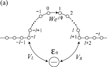
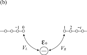
Figure 1: (a) Model for a mesoscopic ring with an embedded quantum dot. A quantum dot with single energy level $\epsilon_{0}$ is connected to two external leads by tunnel couplings, $V_{L}$ and $V_{R}$. There is a barrier with tunnel coupling $W$ on an arm of the ring which directly connects the two leads (reference arm). The ring and two leads are described by a one-dimensional tight-binding model. The magnetic flux penetrating the ring is represented by the AB phase $\phi$ at the tunnel barrier. (b) Model for a quantum dot coupled to two leads without the reference arm.

II.1 Model Hamiltonian

Our model is depicted in Fig. 1(a). A quantum dot with a single energy level, $\epsilon_{0}$, is connected to two external leads by tunnel couplings, $V_{L}$ and $V_{R}$. A barrier with tunnel coupling $W$ is put on an arm of the ring which directly connects the two leads (reference arm). The reference arm and two leads are represented by a one-dimensional tight-binding model with transfer integral $-t$ and lattice constant $a$. The ring size is defined as $L=(2l+1)a$, where $2l$ is the number of sites on the reference arm.

When a magnetic flux $\Phi$ penetrates the ring, the AB phase is given by $\phi=2\pi\Phi/\Phi_{0}$ with the flux quantum $\Phi_{0}=h/e$. The AB interference effect is considered as the AB phase at the tunnel barrier without the loss of generality.com0 The Hamiltonian of the system reads

$$H^{(0)} = H_{\mathrm{dot}}+H_{\mathrm{leads+ring}}+H_{\mathrm{T}},$$ (3)

$$H_{\mathrm{dot}} = \sum_{\sigma=\uparrow,\downarrow}\epsilon_{0}d^{\dagger}_{\sigma}d_{\sigma}+U\hat{n}_{\uparrow}\hat{n}_{\downarrow},$$ (4)

$$H_{\mathrm{leads+ring}} = \sum_{i\neq 0}\sum_{\sigma}(-ta^{\dagger}_{i+1,\sigma}a_{i,\sigma}+\mathrm{h.c}.)$$ (5)

$$+\sum_{\sigma}(We^{i\phi}a^{\dagger}_{1,\sigma}a_{0,\sigma}+\mathrm{h.c}.),$$

$$H_{\mathrm{T}} = \sum_{\sigma}(V_{L}d^{\dagger}_{\sigma}a_{-l,\sigma}+V_{R}d^{\dagger}_{\sigma}a_{l+1,\sigma}+\mathrm{h.c}.),$$ (6)

where $d_{\sigma}^{\dagger}$ and $d_{\sigma}$ are creation and annihilation operators, respectively, of an electron in the quantum dot with spin $\sigma$. $a_{i,\sigma}^{\dagger}$ and $a_{i,\sigma}$ are those at site $i$ with spin $\sigma$ in the leads or ring. $U$ is the electron-electron interaction in the quantum dot. $\hat{n}_{\sigma}=d^{\dagger}_{\sigma}d_{\sigma}$ is the number operator in the dot with spin $\sigma$.

In the leads, the energy dispersion is linearlized around the Fermi energy $\epsilon_{\mathrm{F}}$: $\epsilon_{k}=-2t\cos ka$ is replaced by $\epsilon_{k}=\hbar v_{\mathrm{F}}(|k|-k_{\mathrm{F}})$ with the Fermi wavenumber $k_{\mathrm{F}}$, as shown in Fig. 2, where $v_{\mathrm{F}}=(2ta/\hbar)\sin k_{\mathrm{F}}a$. We assume that $\epsilon_{\mathrm{F}}\simeq 0$ [$k_{\mathrm{F}}\simeq\pi/(2a)$] and set the Fermi energy to be $\epsilon_{\mathrm{F}}=0$. Half of the bandwidth is $D_{0}=\hbar v_{\mathrm{F}}k_{\mathrm{F}}$ ($-2k_{\mathrm{F}}<k\leq 2k_{\mathrm{F}}$). The density of states in a lead is constant; $\rho(\epsilon_{k})=Na/(\pi\hbar v_{\mathrm{F}})$, where $N$ is the number of sites in the lead. This simplification is justified since the wide-band limit is taken later.

For examining the Kondo effect, we focus on the Coulomb blockade regime with one electron in the quantum dot, which satisfies the conditions of $-\epsilon_{0}$, $\epsilon_{0}+U\gg\Gamma$, $k_{\mathrm{B}}T$. $\Gamma=\Gamma_{L}+\Gamma_{R}$ is the level broadening in the quantum dot, where $\Gamma_{\alpha}=\pi\nu_{0}V_{\alpha}^{2}$ with $\nu_{0}=1/(\pi t)$ being the local density of states at the end of semi-infinite leads at the Fermi level $\epsilon_{\mathrm{F}}=0$. The background transmission probability through the reference arm is given by $T_{\mathrm{b}}=4x/(1+x)^{2}$ with $x=(W/t)^{2}$.

For comparison, we examine another model without the reference arm: a quantum dot with single energy level $\epsilon_{0}$ is connected to two external leads by tunnel couplings, $V_{L}$ and $V_{R}$, as shown in Fig. 1(b).

Figure 2: The energy dispersion in the external leads in Figs. 1(a) and (b): $\epsilon_{k}=\hbar v_{\mathrm{F}}(|k|-k_{\mathrm{F}})$ for $-2k_{\mathrm{F}}<k\leq 2k_{\mathrm{F}}$. The half of the bandwidth is given by $D_{0}=\hbar v_{\mathrm{F}}k_{\mathrm{F}}$.

II.2 Equivalent model

From the Hamiltonian in Eq. (3), we construct an equivalent model in which a quantum dot is coupled to a single lead. First, we diagonalize the Hamiltonian $H_{\mathrm{leads+ring}}$ for the outer region of the quantum dot. There are two eigenstates for a given wavenumber $|k|$.

$$|\psi_{k,\rightarrow}\rangle = \sum_{n\leq 0}(e^{ikna}+r_{k}e^{-ikna})|n\rangle+\sum_{n\geq 1}t_{k}e^{ik(n-1)a}e^{i\phi}|n\rangle,$$ (7)

$$|\psi_{k,\leftarrow}\rangle = \sum_{n\leq 0}t_{k}e^{-ikna}|n\rangle+\sum_{n\geq 1}[e^{-ik(n-1)a}+r_{k}e^{ik(n-1)a}]e^{i\phi}|n\rangle,$$ (8)

apart from a normalization factor, $1/\sqrt{2N}$. Here,

$$t_{k}=-\frac{\sqrt{x}(1-e^{2ika})e^{ika}}{1-xe^{2ika}},\ r_{k}=-\frac{(1-x)e^{2ika}}{1-xe^{2ika}},$$ (9)

and $|n\rangle$ is the Wannier function at site $n$. $|\psi_{k,\rightarrow}\rangle$ ($|\psi_{k,\leftarrow}\rangle$) represents the state that an incident plane wave from the left (right) is partly reflected to the left (right) and partly transmitted to the right (left). The spin index is omitted for now. We perform a unitary transformation for these modes

$$\left(\begin{array}[]{cc}|\psi_{k}\rangle&|\bar{\psi}_{k}\rangle\end{array}\right)=\left(\begin{array}[]{cc}|\psi_{k,\rightarrow}\rangle&|\psi_{k,\leftarrow}\rangle\end{array}\right)\left(\begin{array}[]{cc}A_{k}&-B_{k}^{*}\\ B_{k}&A_{k}^{*}\end{array}\right),$$ (10)

where $A_{k}$ and $B_{k}$ are determined such that $\langle d|H_{\mathrm{T}}|\bar{\psi}_{k}\rangle=0$ with dot state $|d\rangle$. As a result, mode $|\psi_{k}\rangle$ is coupled to the dot via $H_{\mathrm{T}}$, whereas mode $|\bar{\psi}_{k}\rangle$ is completely decoupled.

Neglecting the decoupled mode, we obtain a model equivalent to the Hamiltonian in Eq. (3) in order to discuss the Kondo effect. The tunnel coupling of $|\psi_{k}\rangle$ to the quantum dot is described by

$$|\langle d|H_{\mathrm{T}}|\psi_{k}\rangle|^{2} = \frac{2V^{2}}{N}\left\{1-\frac{1-x}{(1+x)^{2}}\frac{1}{1-T_{\mathrm{b}}(\epsilon_{k}/D_{0})^{2}}[\cos 2k(l+1)a-x\cos 2kla]\right.$$ (11)

$$-2\left.\frac{\sqrt{\alpha x}\cos\phi}{(1+x)^{2}}\frac{\sqrt{1-(\epsilon_{k}/D_{0})^{2}}}{1-T_{\mathrm{b}}(\epsilon_{k}/D_{0})^{2}}[\sin 2k(l+1)a-x\sin 2kla]\right\}\equiv|V_{0}(\epsilon_{k})|^{2},$$

where $\alpha=4\Gamma_{L}\Gamma_{R}/(\Gamma_{L}+\Gamma_{R})^{2}$ is the asymmetric factor for the tunnel couplings of the quantum dot. We find that

$$|V_{0}(\epsilon_{k})|^{2} = \frac{2V^{2}}{N}\left(1+\frac{1-x}{1+x}\sin kL-\frac{2}{1+x}\sqrt{\alpha x}\cos\phi\cos kL\right),$$ (12)

in a wide-band limit, where half of the bandwidth $D_{0}$ is much larger than $|\epsilon_{0}|$. Since the strength of tunnel coupling between the leads and dot is characterized by $\rho(\epsilon_{k})|V_{0}(\epsilon_{k})|^{2}$, we can choose the density of states in the lead, $\nu(\epsilon_{k})$, in such a way that $\nu(\epsilon_{k})V^{2}=\rho(\epsilon_{k})|V_{0}(\epsilon_{k})|^{2}$ with $V=\sqrt{V_{L}^{2}+V_{R}^{2}}$. Then the Hamiltonian is written as

$$H=\sum_{\sigma}\epsilon_{0}d^{\dagger}_{\sigma}d_{\sigma}+U\hat{n}_{\uparrow}\hat{n}_{\downarrow}+\sum_{k,\sigma}\epsilon_{k}a^{\dagger}_{k,\sigma}a_{k,\sigma}+\sum_{k,\sigma}V(d^{\dagger}_{\sigma}a_{k,\sigma}+\mathrm{h.c}.),$$ (13)

with the density of states in the lead

$$\nu(\epsilon_{k})=\nu_{0}\left[1+\sqrt{1-T_{\mathrm{b}}}\sin\frac{\epsilon_{k}+D_{0}}{\epsilon_{\mathrm{T}}}-P(\phi)\cos\frac{\epsilon_{k}+D_{0}}{\epsilon_{\mathrm{T}}}\right]$$ (14)

for $-D_{0}\leq\epsilon_{k}\leq D_{0}$, where $\epsilon_{\mathrm{T}}=\hbar v_{\mathrm{F}}/L$ is the Thouless energy for ballistic systems,Altland or energy level spacing in an isolated ring. Here,

$$P(\phi)=\sqrt{\alpha T_{\mathrm{b}}}\cos\phi.$$ (15)

$|P(\phi)|\leq 1$ since $0<\alpha$, $T_{\mathrm{b}}\leq 1$. All the interference effects in the ring, i.e., the AB oscillation and the higher harmonics, are involved in the density of states in Eq. (14). It oscillates with the period of $\epsilon_{\mathrm{T}}$, as schematically shown in Fig. 3. We assume that $\epsilon_{\mathrm{T}}\ll D_{0}$. The amplitude and phase of $\nu(\epsilon_{k})$ depend on the magnetic flux penetrating the ring through $P(\phi)$.

Figure 3: Schematic drawing of the density of states $\nu(\epsilon_{k})$ in a lead in the reduced model. It oscillates with the period $\epsilon_{\mathrm{T}}$. Its amplitude and phase depend on the magnetic flux penetrating the ring through $P(\phi)$ in Eq. (15).

III Case of $U\rightarrow\infty$

The Hamiltonian (13) in the reduced model is analyzed by the “poor man’s” scaling method.Anderson We examine the case of $U\rightarrow\infty$ in this section. The scaling procedure consists of two stages.Haldane On the first stage of the scaling, the charge fluctuation is taken into account. We reduce the energy scale from bandwidth $D_{0}$ until the charge fluctuation is quenched at $D=D_{1}$. By integrating out the excitations in the energy range of $D_{1}<D<D_{0}$, the energy level $\epsilon_{0}$ in the dot is renormalized to $\tilde{\epsilon}_{0}$ ($D_{1}\simeq|\tilde{\epsilon}_{0}|$). On the second stage, we consider the spin fluctuation at low energies of $D<D_{1}$. We evaluate the Kondo temperature, using the Kondo Hamiltonian.

In Appendix A, we illustrate the scaling procedure for the model in Fig. 1(b) in which a quantum dot is connected to two leads without the reference arm. In its equivalent model, a quantum dot is coupled to a lead, in which the tunnel coupling is $V=\sqrt{V_{L}^{2}+V_{R}^{2}}$ and the density of states in the lead is $\nu(\epsilon_{k})=\nu_{0}$.Glazman0 The first stage scaling yields the renormalized energy level

$$\tilde{\epsilon}_{0}^{(0)}\simeq\epsilon_{0}+\nu_{0}V^{2}\ln\frac{D_{0}}{|\epsilon_{0}|}.$$ (16)

On the second stage, the Kondo temperature is evaluated as

$$T_{\mathrm{K}}^{(0)}\simeq|\epsilon_{0}|\exp\left(-\frac{1}{2\nu_{0}J}\right),$$ (17)

where the exchange coupling is $J=V^{2}/|\tilde{\epsilon}_{0}^{(0)}|$.

III.1 Energy level renormalization

Let us start the first stage of scaling using the reduced model obtained in Sec. II.B. The energy level in the quantum dot is evaluated by $\epsilon_{0}=E_{1}-E_{0}$, where $E_{0}$ is the energy of the empty state and $E_{1}$ is that of the singly occupied state. Reducing the bandwidth from $D$ to $D-|dD|$, they are renormalized to $E_{0}+dE_{0}$ and $E_{1}+dE_{1}$, where

$$dE_{0} = -\frac{2V^{2}\nu(-D)}{D+E_{1}-E_{0}}|dD|,$$

$$dE_{1} = -\frac{V^{2}\nu(D)}{D+E_{0}-E_{1}}|dD|,$$

within the second-order perturbation with respect to tunnel coupling $V$. For $D\gg|E_{1}-E_{0}|$, they yield the scaling equation for the energy level

$$\frac{d\epsilon_{0}}{d\ln D}=V^{2}\left[\nu(D)-2\nu(-D)\right].$$ (18)

Using the density of states $\nu(\epsilon_{k})$ in Eq. (14) and relation of $D_{0}/\epsilon_{\mathrm{T}}=k_{\mathrm{F}}L$, we obtain

$$\frac{d\epsilon_{0}}{d\ln D} = -\nu_{0}V^{2}\left[1+F_{1}(k_{\mathrm{F}}L,\phi)\cos\frac{D}{\epsilon_{\mathrm{T}}}+3F_{2}(k_{\mathrm{F}}L,\phi)\sin\frac{D}{\epsilon_{\mathrm{T}}}\right],$$ (19)

where

$$F_{1}(k_{\mathrm{F}}L,\phi) = \frac{\nu(\epsilon_{\mathrm{F}})-\nu_{0}}{\nu_{0}}$$ (20)

$$= \sqrt{1-T_{\mathrm{b}}}\sin k_{\mathrm{F}}L-P(\phi)\cos k_{\mathrm{F}}L$$

and

$$F_{2}(k_{\mathrm{F}}L,\phi)=F_{1}(k_{\mathrm{F}}L+\pi/2,\phi).$$ (21)

By the integration of Eq. (19) from $D_{0}$ to $D_{1}$, we obtain the renormalized energy level

$$\tilde{\epsilon}_{0} = \epsilon_{0}+\nu_{0}V^{2}\Biggl{\{}\ln\frac{D_{0}}{D_{1}}-F_{1}(k_{\mathrm{F}}L,\phi)\left[\mathrm{Ci}\left(\frac{D_{1}}{\epsilon_{\mathrm{T}}}\right)-\mathrm{Ci}\left(\frac{D_{0}}{\epsilon_{\mathrm{T}}}\right)\right]$$ (22)

$$-3F_{2}(k_{\mathrm{F}}L,\phi)\left[\mathrm{Si}\left(\frac{D_{1}}{\epsilon_{\mathrm{T}}}\right)-\mathrm{Si}\left(\frac{D_{0}}{\epsilon_{\mathrm{T}}}\right)\right]\Biggr{\}},$$

where

$$\mathrm{Si}(x)\equiv\int^{x}_{0}d\xi\frac{\sin{\xi}}{\xi},$$

$$\mathrm{Ci}(x)\equiv\int_{-\infty}^{x}d\xi\frac{\cos{\xi}}{\xi},$$

and $D_{1}\simeq|\tilde{\epsilon}_{0}|$. Since $\Gamma=\pi\nu_{0}V^{2}\ll-\epsilon_{0}\ll D_{0}$, $D_{1}\simeq-\epsilon_{0}$. Thus

$$\tilde{\epsilon}_{0} \simeq \epsilon_{0}+\nu_{0}V^{2}\left\{\ln\frac{D_{0}}{|\epsilon_{0}|}-F_{1}(k_{\mathrm{F}}L,\phi)\mathrm{Ci}\left(\frac{|\epsilon_{0}|}{\epsilon_{\mathrm{T}}}\right)-3F_{2}(k_{\mathrm{F}}L,\phi)\left[\mathrm{Si}\left(\frac{|\epsilon_{0}|}{\epsilon_{\mathrm{T}}}\right)-\frac{\pi}{2}\right]\right\}$$ (23)

since $D_{0}\gg\epsilon_{\mathrm{T}}$. Here, we have used asymptotic forms of $\mathrm{Si}(x)\sim{\pi}/{2}+{\cos x}/{x}$ and $\mathrm{Ci}(x)\sim{\sin x}/{x}$ for $x\rightarrow\infty$.

From Eq. (23), we derive the renormalized level in two situations, (i) $|\epsilon_{0}|\gg\epsilon_{\mathrm{T}}$ and (ii) $|\epsilon_{0}|\ll\epsilon_{\mathrm{T}}$. In situation (i), we find

$$\tilde{\epsilon}_{0}(\phi)\simeq\tilde{\epsilon}_{0}^{(0)},$$ (24)

using the asymptotic forms of $\mathrm{Si}(x)$ and $\mathrm{Ci}(x)$ at $x\rightarrow\infty$ again. $\tilde{\epsilon}_{0}^{(0)}$ is given by Eq. (16). In this situation, the oscillating part of $\nu(\epsilon_{k})$ in Eq. (14) is averaged out in the integration of the scaling equation (19). As a result, the renormalization of energy level is not influenced by the AB interference effect in the ring.

In situation (ii),

$$\tilde{\epsilon}_{0}(\phi) = \tilde{\epsilon}_{0}^{(0)}-\nu_{0}V^{2}\sqrt{1-T_{\mathrm{b}}}\left[\frac{3\pi}{2}\cos k_{\mathrm{F}}L+\left(\gamma+\ln\frac{|\epsilon_{0}|}{\epsilon_{\mathrm{T}}}\right)\sin k_{\mathrm{F}}L\right]$$ (25)

$$-\nu_{0}V^{2}P(\phi)\left[\frac{3\pi}{2}\sin k_{\mathrm{F}}L-\left(\gamma+\ln\frac{|\epsilon_{0}|}{\epsilon_{\mathrm{T}}}\right)\cos k_{\mathrm{F}}L\right],$$

using the other asymptotic forms of $\mathrm{Si}(x)\sim x$ and $\mathrm{Ci}(x)\sim\gamma+\ln x$ for $x\rightarrow 0$. $\gamma\simeq 0.5772$ is the Euler’s constant. In this situation, the renormalized level is modulated by the AB interference effect.

Conditions (i) and (ii) are rewritten as $L\gg L_{\mathrm{c}}$ and $L\ll L_{\mathrm{c}}$, respectively, where $L_{\mathrm{c}}=\hbar v_{\mathrm{F}}/|\epsilon_{0}|$. $L_{\mathrm{c}}$ is the screening length of charge fluctuation. When $L\gg L_{\mathrm{c}}$, the screening of charge fluctuation is hardly influenced by the AB interference effect. Thus the renormalization of energy level is independent of magnetic flux, as shown in Eq. (24). When $L\ll L_{\mathrm{c}}$, the screening is modulated by $\phi$ and also changed by $k_{\mathrm{F}}L$, following Eq. (25).

III.2 Evaluation of Kondo temperature

On the second stage of scaling, we start from the Hamiltonian (13) with renormalized energy level $\tilde{\epsilon}_{0}$ and bandwidth $D_{1}\simeq|\epsilon_{0}|$. To describe the spin fluctuation at the low-energy scale of $D\ll D_{1}$, we make the Kondo Hamiltonian via the Schrieffer-Wolff transformation

$$H_{\mathrm{Kondo}} = \sum_{k,\sigma}\epsilon_{k\sigma}a^{\dagger}_{k\sigma}a_{k\sigma}+H_{J}+H_{K},$$ (26)

$$H_{J} = J\sum_{k^{\prime},k}[S^{+}a^{\dagger}_{k^{\prime}\downarrow}a_{k\uparrow}+S^{-}a^{\dagger}_{k^{\prime}\uparrow}a^{\dagger}_{k\downarrow}+S_{z}(a^{\dagger}_{k^{\prime}\uparrow}a_{k\uparrow}-a^{\dagger}_{k^{\prime}\downarrow}a_{k\downarrow})],$$ (27)

$$H_{K} = K\sum_{k^{\prime},k}\sum_{\sigma}a^{\dagger}_{k^{\prime}\sigma}a_{k\sigma},$$ (28)

where $S^{+}=d^{\dagger}_{\uparrow}d_{\downarrow}$, $S^{-}=d^{\dagger}_{\downarrow}d_{\uparrow}$ and $S_{z}=(d^{\dagger}_{\uparrow}d_{\uparrow}-d^{\dagger}_{\downarrow}d_{\downarrow})/2$ are the spin operators in the quantum dot. $H_{J}$ indicates the exchange coupling between the localized spin and conduction electrons in the lead, whereas $H_{K}$ represents the potential scattering of the conduction electrons by the quantum dot. The coupling constants are

$$J=\frac{V^{2}}{|\tilde{\epsilon}_{0}|}$$ (29)

and

$$K=\frac{V^{2}}{2|\tilde{\epsilon}_{0}|}.$$ (30)

Note that they depend on $\phi$ through $\tilde{\epsilon}_{0}$ in Eq. (25) in the situation of $L\ll L_{\mathrm{c}}$, whereas they do not in the situation of $L\gg L_{\mathrm{c}}$. The density of states in the lead is given by $\nu(\epsilon_{k})$ in Eq. (14).

By changing the bandwidth, we renormalize the coupling constants $J$ and $K$ so as not to change the low-energy physics within the second-order perturbation with respect to $H_{J}$ and $H_{K}$. The coupling constants follow the scaling equations

$$\frac{dJ}{d\ln D} = -J^{2}\left[\nu(D)+\nu(-D)\right]-2JK\left[\nu(D)-\nu(-D)\right],$$ (31)

$$\frac{dK}{d\ln D} = -\left(\frac{3J^{2}}{4}+K^{2}\right)\left[\nu(D)-\nu(-D)\right].$$ (32)

Using the density of states $\nu(\epsilon_{k})$ in Eq. (14), we obtain

$$\frac{dJ}{d\ln D} = -2\nu_{0}J^{2}-2\nu_{0}J^{2}F_{1}(k_{\mathrm{F}}L,\phi)\cos\frac{D}{\epsilon_{\mathrm{T}}}+4\nu_{0}JKF_{2}(k_{\mathrm{F}}L,\phi)\sin\frac{D}{\epsilon_{\mathrm{T}}},$$ (33)

$$\frac{dK}{d\ln D} = 2\nu_{0}\left(\frac{3}{4}J^{2}+4K^{2}\right)F_{2}(k_{\mathrm{F}}L,\phi)\sin\frac{D}{\epsilon_{\mathrm{T}}},$$ (34)

where $F_{1}(k_{\mathrm{F}}L,\phi)$ and $F_{2}(k_{\mathrm{F}}L,\phi)$ are given by Eqs. (20) and (21). The energy scale $D$ where the fixed point of strong coupling is reached determines the Kondo temperature.

We evaluate $T_{\mathrm{K}}$ in the following procedures. First, scaling equations (33) and (34) are analyzed in two extreme cases. In the case of $D\gg\epsilon_{\mathrm{T}}$, the oscillating part of the density of states $\nu(\epsilon_{k})$ is averaged out in the integration. Then the scaling equations are effectively rewritten as

$$\frac{dJ}{d\ln D} \simeq -2\nu_{0}J^{2},$$ (35)

$$\frac{dK}{d\ln D} \simeq 0.$$ (36)

Thus the potential scattering is irrelevant to the Kondo effect in this case. In the case of $D\ll\epsilon_{\mathrm{T}}$, the last term is much smaller than the other terms on the right side of Eq. (33). Hence the exchange coupling $J$ is renormalized by

$$\frac{dJ}{d\ln D}\simeq-2\nu_{0}\left[1+F_{1}(k_{\mathrm{F}}L,\phi)\cos\frac{D}{\epsilon_{\mathrm{T}}}\right]J^{2}.$$ (37)

The coupling constant $K$ is also renormalized although its development is slower than that of $J$ by the factor of $D/\epsilon_{\mathrm{T}}$. [As $D\rightarrow T_{\mathrm{K}}$, $J$ and $K$ become $|K|/J=$constant ($\ll 1$) at the fixed point of Eqs. (33) and (34), as shown in Appendix C.]

Using Eqs. (35) and (37), we evaluate the Kondo temperature in three situations, (i) $\epsilon_{\mathrm{T}}\ll T_{\mathrm{K}}\ll|\epsilon_{0}|$, (ii) $T_{\mathrm{K}}\ll\epsilon_{\mathrm{T}}\ll|\epsilon_{0}|$, and (iii) $T_{\mathrm{K}}\ll|\epsilon_{0}|\ll\epsilon_{\mathrm{T}}$. The conditions correspond to (i) $L_{\rm c}\ll L_{\rm K}\ll L$, (ii) $L_{\rm c}\ll L\ll L_{\rm K}$, and (iii) $L\ll L_{\rm c}\ll L_{\rm K}$, respectively, where $L_{\rm K}=v_{\rm F}\hbar/T_{\rm K}$ is the screening length of spin fluctuation, i.e. size of the Kondo screening cloud.

In situation (i), the scaling equation (35) can be applicable until the scaling ends at $D\simeq T_{\mathrm{K}}$, where $J\rightarrow\infty$. By integrating the equation from $D_{1}\simeq|\epsilon_{0}|$ to $T_{\mathrm{K}}$, we obtain

$$T_{\mathrm{K}}\simeq|\epsilon_{0}|\exp\left(-\frac{1}{2\nu_{0}J}\right).$$ (38)

This is identical to $T_{\mathrm{K}}^{(0)}$ in Eq. (17). The AB interference effect does not affect the energy-level renormalization nor Kondo temperature when the ring size $L$ is much larger than both the screening length of charge fluctuation $L_{\rm c}$ and that of spin fluctuation $L_{\rm K}$.

In situation (iii), the scaling equation (37) is valid in the whole scaling region of $T_{\mathrm{K}}<D<D_{1}$, which yields

$$T_{\mathrm{K}}\simeq|\epsilon_{0}|\exp\left[-\frac{\chi(\phi)}{2\nu_{0}J}\right],$$ (39)

where $\chi(\phi)=\left[1+F_{1}(k_{\mathrm{F}}L,\phi)\right]^{-1}=\nu_{0}/\nu(\epsilon_{\mathrm{F}})$, or

$$\chi(\phi)=\left[1+\sqrt{1-T_{\mathrm{b}}}\sin k_{\mathrm{F}}L-P(\phi)\cos k_{\mathrm{F}}L\right]^{-1}.$$ (40)

Using the renormlized energy in Eq. (25), we find

$$T_{\mathrm{K}}(\phi) \simeq |\epsilon_{0}|\left(\frac{T_{\mathrm{K}}^{(0)}}{|\epsilon_{0}|}\right)^{\chi(\phi)|\tilde{\epsilon}_{0}(\phi)/\tilde{\epsilon}_{0}^{(0)}|}.$$ (41)

In this situation, both $\tilde{\epsilon}_{0}(\phi)$ and $T_{\mathrm{K}}(\phi)$ are modulated by the magnetic flux since $L$ is smaller than both the screening lengths.

In situation (ii), $T_{\mathrm{K}}\ll\epsilon_{\mathrm{T}}\ll|\epsilon_{0}|$. The coupling constant $J$ is renormalized following Eq. (35) when $D$ is reduced from $D_{1}$ to $\epsilon_{\mathrm{T}}$, and following Eq. (37) when $D$ is reduced from $\epsilon_{\mathrm{T}}$ to $T_{\rm K}$. We match the solutions of the respective equations aroud $D\simeq\epsilon_{\mathrm{T}}$ and obtain

$$T_{\mathrm{K}}(\phi)\simeq\epsilon_{\mathrm{T}}e^{\gamma}\left(\frac{T_{\mathrm{K}}^{(0)}}{\epsilon_{\mathrm{T}}e^{\gamma}}\right)^{\chi(\phi)}.$$ (42)

In this situation, the Kondo temperature reflects the AB interference effect since the ring size $L$ is smaller than the Kondo screening length $L_{\rm K}$, whereas the energy-level renormalization does not since $L$ is larger than $L_{\rm c}$.

The obtained results of $T_{\mathrm{K}}$ are plotted in Fig. 4, as a function $\phi$, with (a) $k_{\mathrm{F}}L=0$ $\mathrm{mod}\ 2\pi$ and (b) $k_{\mathrm{F}}L=\pi$ $\mathrm{mod}\ 2\pi$. Since $T_{\mathrm{K}}(\phi)$ depends on $\phi$ through $P(\phi)$ in Eq. (15), it is a periodic function of $\phi$ and satisfies $T_{\mathrm{K}}(\phi)=T_{\mathrm{K}}(-\phi)$. $T_{\mathrm{K}}$ is significantly modulated by $\phi$ in situations (ii) and (iii), as shown by broken and solid lines, respectively. In these situations, $T_{\mathrm{K}}(\phi)$ is also changed by $k_{\mathrm{F}}L$ since the interference pattern is modified with $k_{\mathrm{F}}L$. In situation (i), $T_{\mathrm{K}}(\phi)=T_{\mathrm{K}}^{(0)}$, irrespectively of $\phi$ and $k_{\mathrm{F}}L$ (dotted line).

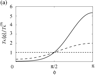
Figure 4: The Kondo temperature $T_{\mathrm{K}}$ as a function of AB phase $\phi$ of the magnetic flux penetrating the ring, in the case of $U\rightarrow\infty$. (a) $k_{\mathrm{F}}L=0$ $\mathrm{mod}\ 2\pi$ and (b) $\pi$ $\mathrm{mod}\ 2\pi$, where $L$ is the ring size and $k_{\mathrm{F}}$ is the Fermi wavenumber. $T_{\mathrm{K}}$ is normalized by $T_{\mathrm{K}}^{(0)}$ in Eq. (17). Situations (i) $L_{\rm c}\ll L_{\rm K}\ll L$, (ii) $L_{\rm c}\ll L\ll L_{\rm K}$, and (iii) $L\ll L_{\rm c}\ll L_{\rm K}$ are denoted by dotted, broken, and solid lines, respectively. In situation (i), $T_{\mathrm{K}}=T_{\mathrm{K}}^{(0)}$, irrespectively of the AB phase $\phi$.

IV Vicinity of electron-hole symmetry

In this section, we present the scaling analysis in the vicinity of electron-hole symmetry; $-\epsilon_{0}\simeq\epsilon_{0}+U$ (more precisely, $|2\epsilon_{0}+U|<\Gamma$). The scaling procedure is almost the same as in the previous section. On the first stage of scaling, we consider the energy level for the first electron in the quantum dot, $\epsilon_{0}$, and that for the second electron, $\epsilon_{1}=\epsilon_{0}+U$.

In Appendix A, the scaling analysis is given for the model in Fig. 1(b) without the reference arm. On the first stage, the energy levels are not renormalized;

$$\tilde{\epsilon}_{i}^{(0)}\simeq\epsilon_{i}$$ (43)

for $i=1,2$. The second stage yields the Kondo temperature as

$$T_{\mathrm{K}}^{(0)}=|\epsilon_{0}|\exp\left(-\frac{1}{2\nu_{0}J}\right),$$ (44)

where $J={V^{2}}\left[{|\epsilon_{0}|^{-1}}+(\epsilon_{0}+U)^{-1}\right]$. Note that $T_{\mathrm{K}}^{(0)}$ in Eq. (44) is used in this section, which is different from $T_{\mathrm{K}}^{(0)}$ in the previous section [$J$ is not identical in Eqs. (17) and (44)].

IV.1 Energy level renormalization

On the first stage of scaling, the charge fluctuation is taken into account. The energy levels in the quantum dot are given by $\epsilon_{0}=E_{1}-E_{0}$ for the first electron and $\epsilon_{1}=E_{2}-E_{1}$ for the second electron, where $E_{0}$, $E_{1}$, and $E_{2}$ are the energies of the empty state, singly occupied state, and doubly occupied state in the quantum dot, respectively. When the bandwidth is reduced from $D$ to $D-|dD|$, $E_{j}$ ($j=0,1,2$) are renormalized to $E_{j}+dE_{j}$ with

$$dE_{0} = -\frac{2V^{2}\nu(-D)}{D+E_{1}-E_{0}}|dD|,$$

$$dE_{1} = -\left[\frac{V^{2}\nu(D)}{D+E_{0}-E_{1}}+\frac{V^{2}\nu(-D)}{D+E_{2}-E_{1}}\right]|dD|,$$

$$dE_{2} = -\frac{2V^{2}\nu(D)}{D+E_{1}-E_{2}}|dD|,$$

within the second-order perturbation with respect to tunnel coupling $V$. For $D\gg|E_{1}-E_{0}|$, $|E_{2}-E_{1}|$, they yield the scaling equations for the energy levels

$$\frac{d\epsilon_{0}}{d\ln D}=\frac{d\epsilon_{1}}{d\ln D}=2\nu_{0}V^{2}F_{2}(k_{\mathrm{F}}L,\phi)\sin\frac{D}{\epsilon_{\mathrm{T}}},$$ (45)

where $F_{2}(k_{\mathrm{F}}L,\phi)$ is given by Eq. (21) in the previous section.

By the integration of Eq. (45) from $D_{0}$ to $D_{1}$, we obtain the renormalized energy levels

$$\tilde{\epsilon}_{i} = \epsilon_{i}+2\nu_{0}V^{2}F_{2}(k_{\mathrm{F}}L,\phi)\left[\mathrm{Si}\left(\frac{D_{1}}{\epsilon_{\mathrm{T}}}\right)-\frac{\pi}{2}\right],$$ (46)

for $i=0,1$, with $D_{1}\simeq\mathrm{max}(-\tilde{\epsilon}_{0},\tilde{\epsilon}_{1})$. In the situation considered, $D_{1}\simeq-\tilde{\epsilon}_{0}\simeq\tilde{\epsilon}_{1}$.

From Eq. (46), we derive the renormalized level in two situations, (i) $|\epsilon_{0}|\gg\epsilon_{\mathrm{T}}$ and (ii) $|\epsilon_{0}|\ll\epsilon_{\mathrm{T}}$. They correspond to (i) $L\gg L_{\mathrm{c}}$ and (ii) $L\ll L_{\mathrm{c}}$, respectively, with $L_{\mathrm{c}}=\hbar v_{\mathrm{F}}/|\epsilon_{0}|$ is the screening length of charge fluctuation. In situation (i), we find

$$\tilde{\epsilon}_{0} \simeq \epsilon_{0},$$ (47)

$$\tilde{\epsilon}_{1} \simeq \epsilon_{1}=\epsilon_{0}+U.$$ (48)

The AB interference effect does not work on the level renormalization since the ring size $L$ is larger than the screening length of charge fluctuation.

In situation (ii), the renormalized level is modulated by the AB interference effect as

$$\tilde{\epsilon}_{i} \simeq \epsilon_{i}-\pi\nu_{0}V^{2}F_{2}(k_{\mathrm{F}}L,\phi)$$ (49)

$$= \epsilon_{i}-\pi\nu_{0}V^{2}\left[\sqrt{1-T_{\mathrm{b}}}\cos k_{\mathrm{F}}L+P(\phi)\sin k_{\mathrm{F}}L\right].$$

IV.2 Evaluation of Kondo temperature

On the second stage, we derive the Kondo Hamiltonian $H_{\mathrm{Kondo}}$ via the Schrieffer-Wolff transformation. $H_{\mathrm{Kondo}}$ is in the same form as in Eq. (26) in the previous section, with coupling constants of

$$J = {V^{2}}\left(\frac{1}{|\tilde{\epsilon}_{0}|}+\frac{1}{\tilde{\epsilon}_{1}}\right),$$ (50)

$$K = \frac{V^{2}}{2}\left(\frac{1}{|\tilde{\epsilon}_{0}|}-\frac{1}{\tilde{\epsilon}_{1}}\right).$$ (51)

The energy levels $\tilde{\epsilon}_{0}$ and $\tilde{\epsilon}_{1}$ are not renormalized when $|\epsilon_{0}|\gg\epsilon_{\mathrm{T}}$, whereas they are given by Eq. (49) when $|\epsilon_{0}|\ll\epsilon_{\mathrm{T}}$. In both the situations, we find

$$J\simeq{V^{2}}\left(\frac{1}{|{\epsilon}_{0}|}+\frac{1}{\epsilon_{0}+U}\right)$$ (52)

to the order of $\Gamma/|\epsilon_{0}|$.

The scaling equations for $J$ and $K$ are derived within the second-order perturbation with respect to $H_{J}$ and $H_{K}$. They are identical to those in the previous section, Eqs. (33) and (34). From the equations, we obtain Eq. (35) in the case of $D\gg\epsilon_{\mathrm{T}}$ and Eq. (37) in the case of $D\ll\epsilon_{\mathrm{T}}$.

We evaluate the Kondo temperature in three situations, (i) $L_{\rm c}\ll L_{\rm K}\ll L$, (ii) $L_{\rm c}\ll L\ll L_{\rm K}$, and (iii) $L\ll L_{\rm c}\ll L_{\rm K}$. In situation (i), $\epsilon_{\mathrm{T}}\ll T_{\mathrm{K}}\ll|\epsilon_{0}|$. The scaling equation (35) yields

$$T_{\mathrm{K}}(\phi)\simeq T_{\mathrm{K}}^{(0)}$$ (53)

which is the Kondo temperature of the model in Fig. 1(b) without the reference arm [Eq. (44)]. The AB interference effect is ineffective on the energy-level renormalization and on the Kondo temperature.

In situation (iii), $T_{\mathrm{K}}\ll|\epsilon_{0}|\ll\epsilon_{\mathrm{T}}$. Then the scaling equation (37) gives us

$$T_{\mathrm{K}}(\phi)\simeq|\epsilon_{0}|\left(\frac{T_{\mathrm{K}}^{(0)}}{|\epsilon_{0}|}\right)^{\chi(\phi)},$$ (54)

where the exponent $\chi(\phi)$ is given by Eq. (40) in the previous section. Since $L$ is smaller than $L_{\rm c}$ and $L_{\rm K}$, both the energy levels and $T_{\mathrm{K}}(\phi)$ are modulated by the magnetic flux. Because the exchange coupling $J$ in Eq. (52) is not influenced by the energy-level renormalization, the expression of $T_{\mathrm{K}}(\phi)$ is simpler than that in Eq. (41) in the previous section.

In situation (ii), $T_{\mathrm{K}}\ll\epsilon_{\mathrm{T}}\ll|\epsilon_{0}|$. $J$ is renormalized by Eq. (35) at $\epsilon_{\mathrm{T}}\ll D\ll D_{1}\simeq|\epsilon_{0}|$ and by Eq. (37) at $T_{\rm K}\ll D\ll\epsilon_{\mathrm{T}}$. We obtain

$$T_{\mathrm{K}}(\phi)\simeq\epsilon_{\mathrm{T}}e^{\gamma}\left(\frac{T_{\mathrm{K}}^{(0)}}{\epsilon_{\mathrm{T}}e^{\gamma}}\right)^{\chi(\phi)}.$$ (55)

Figure 5 shows $T_{\mathrm{K}}(\phi)$ with (a) $k_{\mathrm{F}}L=0$ $\mathrm{mod}\ 2\pi$ and (b) $k_{\mathrm{F}}L=\pi$ $\mathrm{mod}\ 2\pi$. The behavior of $T_{\mathrm{K}}(\phi)$ is qualitatively the same as that in the previous section with $U\rightarrow\infty$. In situations (ii) and (iii), $T_{\mathrm{K}}$ is significantly modulated by $\phi$ (broken and solid lines). It should be mentioned that for a given $k_{\mathrm{F}}L$, the modulation of $T_{\mathrm{K}}(\phi)$ is always larger in situation (iii) than in situation (ii) in the vicinity of electron-hole symmetry [Eqs. (54), (55)]. In situation (i), $T_{\mathrm{K}}=T_{\mathrm{K}}^{(0)}$, irrespectively of $\phi$ and $k_{\mathrm{F}}L$ (dotted line).

Figure 5: The Kondo temperature $T_{\mathrm{K}}$ as a function of AB phase $\phi$ of the magnetic flux penetrating the ring, in the case of electron-hole symmetry, $-\epsilon_{0}=\epsilon_{0}+U$. (a) $k_{\mathrm{F}}L=0$ $\mathrm{mod}\ 2\pi$ and (b) $\pi$ $\mathrm{mod}\ 2\pi$, where $L$ is the ring size and $k_{\mathrm{F}}$ is the Fermi wavenumber. $T_{\mathrm{K}}$ is normalized by $T_{\mathrm{K}}^{(0)}$ in Eq. (44). Situations (i) $L_{\rm c}\ll L_{\rm K}\ll L$, (ii) $L_{\rm c}\ll L\ll L_{\rm K}$, and (iii) $L\ll L_{\rm c}\ll L_{\rm K}$ are denoted by dotted, broken, and solid lines, respectively. In situation (i), $T_{\mathrm{K}}=T_{\mathrm{K}}^{(0)}$, irrespectively of the AB phase $\phi$.

V Conductance

In this section, the conductance is evaluated on the basis of the scaling analysis. First, we calculate the logarithmic corrections in the weak-coupling regime of $T\gg T_{\mathrm{K}}$. The scattering of conduction electrons by a localized spin in the dot is evaluated by the perturbation of $J$ in the Kondo Hamiltonian. Second, we obtain the analytical expression of the conductance in the strong-coupling regime of $T\ll T_{\mathrm{K}}$. We use the Hamiltonian in the strong-coupling fixed point to describe the properties of the Fermi liquid.Glazman The calculations are applicable to both the case of $U\rightarrow\infty$ and the vicinity of electron-hole symmetry if $T_{\mathrm{K}}$ is replaced by the value in respective cases.

V.1 Weak-coupling regime

At $T\gg T_{\mathrm{K}}$, a localized spin $1/2$ still remains in the quantum dot. The scattering of conduction eletrons by the localized spin can be treated by the perturbation with respect to $J$ in the Kondo Hamiltonian in Eq. (26).Hewson We solve a scattering problem for an incident wave of $|\psi_{k,\rightarrow}\rangle$ in Eq. (7) to the lowest order in $J$ (Born approximation). When a localized spin in the quantum dot is in the up-state, $|\mathrm{dot}\uparrow\rangle$, an incident electron has an up- or down-spin, $\sigma=\uparrow$, $\downarrow$. The total wavefunction is written as

$$|\Psi_{\sigma}\rangle=|\psi_{k,\rightarrow};\sigma\rangle\otimes|\mathrm{dot}\uparrow\rangle+{\hat{G}}_{0}(\epsilon_{k})H_{J}\bigl{(}|\psi_{k,\rightarrow};\sigma\rangle\otimes|\mathrm{dot}\uparrow\rangle\bigr{)}$$ (56)

in the Born approximation, where ${\hat{G}}_{0}(\epsilon)$ is the unperturbed Green operator defined by

$$\left[\epsilon-H_{\mathrm{leads+ring}}+i\delta\right]\hat{G}_{0}(\epsilon)=1.$$ (57)

Note that the first term in $H_{\mathrm{Kondo}}$ in Eq. (26) is identical to $H_{\mathrm{leads+ring}}$ in Eq. (5) if the decoupled modes are added. We neglect the potential scattering $H_{K}$ in $H_{\mathrm{Kondo}}$ since it is irrelevant to the Kondo effect, or its logarithmic corrections are much smaller than those of $H_{J}$ (see Sec. III.B).com1 The matrix element of $H_{J}$ on the basis of the Wannier function $|i\rangle$ is given by $\langle i|H_{J}|j\rangle=J(V_{i}V_{j}/V^{2}){\bf S}\cdot{\bf s}$ ($i$, $j=$ $-l$ or $l+1$), where $V_{-l}=V_{L}$, $V_{l+1}=V_{R}$, ${\bf S}$ is the spin operator in the quantum dot, and ${\bf s}$ is that for a conduction electron.

For an incident electron with $\sigma=\uparrow$, the localized spin remains in the up-state. No spin-flip takes place. The transmission probability is $|t_{\uparrow}|^{2}$, where

$$t_{\uparrow} = \bigl{(}\langle l+1;\uparrow|\otimes\langle\mathrm{dot}\uparrow|\bigr{)}|\Psi_{\uparrow}\rangle$$ (58)

$$= \langle l+1|\psi_{k,\rightarrow}\rangle+\frac{1}{2V^{2}}\sum_{i,j=-l,l+1}V_{i}V_{j}\langle l+1|{\hat{G}}_{0}|i\rangle\langle j|\psi_{k,\rightarrow}\rangle.$$

For an incident electron with $\sigma=\downarrow$, there are two scattering processes in absence ($t_{1}$) or present ($t_{2}$) of the spin flip:

$$t_{\downarrow,1} = \bigl{(}\langle l+1;\downarrow|\otimes\langle\mathrm{dot}\uparrow|\bigr{)}|\Psi_{\downarrow}\rangle$$ (59)

$$= \langle l+1|\psi_{k,\rightarrow}\rangle-\frac{1}{2V^{2}}\sum_{i,j=-l,l+1}V_{i}V_{j}\langle l+1|{\hat{G}}_{0}|i\rangle\langle j|\psi_{k,\rightarrow}\rangle,$$

$$t_{\downarrow,2} = \bigl{(}\langle l+1;\uparrow|\otimes\langle\mathrm{dot}\downarrow|\bigr{)}|\Psi_{\downarrow}\rangle$$ (60)

$$= \frac{1}{V^{2}}\sum_{i,j=-l,l+1}V_{i}V_{j}\langle l+1|{\hat{G}}_{0}|i\rangle\langle j|\psi_{k,\rightarrow}\rangle.$$

The transmission probability is given by $|t_{\downarrow,1}|^{2}+|t_{\downarrow,2}|^{2}$. The matrix elements of ${\hat{G}}_{0}(\epsilon_{k})$, $\langle l+1|{\hat{G}}_{0}|-l\rangle$ and $\langle l+1|{\hat{G}}_{0}|l+1\rangle$, are calculated in Appendix D. The conductance is evaluated by averaging over the spin of incident electron $\sigma$:

$$G=\frac{e^{2}}{h}\left.(|t_{\uparrow}|^{2}+|t_{\downarrow,1}|^{2}+|t_{\downarrow,2}|^{2})\right|_{\epsilon_{\mathrm{F}}}.$$ (61)

Finally, $J$ in Eq. (61) is replaced by the renormalized value at $D=k_{\mathrm{B}}T$, $\tilde{J}=[2\nu\ln(T/T_{\mathrm{K}})]^{-1}$. Then we obtain the logarithmic corrections to the conductance

$$G_{\mathrm{K}}=\frac{2e^{2}}{h}\frac{3\pi^{2}}{16\left[\ln\left(T/T_{\mathrm{K}}\right)\right]^{2}}\left[T_{\mathrm{b}}R_{\mathrm{b}}+\frac{\alpha}{4}\left(T_{\mathrm{b}}^{2}+R_{\mathrm{b}}^{2}\right)+\sqrt{\alpha T_{\mathrm{b}}R_{\mathrm{b}}}(T_{\mathrm{b}}+R_{\mathrm{b}})\cos\phi+\frac{\alpha}{2}T_{\mathrm{b}}R_{\mathrm{b}}\cos 2\phi\right],$$ (62)

where $R_{\mathrm{b}}=|\langle-l|\psi_{k,\rightarrow}\rangle|^{2}=2-T_{\mathrm{b}}+2\sqrt{1-T_{\mathrm{b}}}\cos 2kla$. In this approximation, the AB oscillation ($\cos{\phi}$; due to the scattering from site $-l$ to $l+1$) and second harmonics ($\cos{2\phi}$; from site $l+1$ to $-l$) appear, whereas the higher harmonics of the Fano resonance do not. Note that $T_{\mathrm{K}}$ also changes with $\phi$ when $L\ll L_{\mathrm{K}}$.

V.2 Strong-coupling regime

In the strong-coupling regime of $T\ll T_{\mathrm{K}}$, a spin $1/2$ in the quantum dot is fully screened out by the Kondo effect. In this case, we can examine the scattering of $|\psi_{k,\rightarrow}\rangle$ using the Fermi liquid theory. For either spin $\sigma=\uparrow$ or $\downarrow$, the scattered wave is written as

$$|\psi^{\prime}_{k}\rangle=|\psi_{k,\rightarrow}\rangle+{\hat{G}}_{0}(\epsilon_{k})\hat{T}|\psi_{k,\rightarrow}\rangle,$$ (63)

where $\hat{T}$ is the t-matrix of the Kondo model in Eq. (26) and $\hat{G}_{0}(\epsilon_{k})$ is the unperturbed Green operator in Eq. (57). From Eq. (10) in Sec. II.B, the incident wave $|\psi_{k,\rightarrow}\rangle$ consists of two parts:

$$|\psi_{k,\rightarrow}\rangle=A_{k}^{\ast}|\psi_{k}\rangle-B_{k}|\bar{\psi}_{k}\rangle,$$ (64)

where $|\psi_{k}\rangle$ is scattered by $H_{J}+H_{K}$ while $|\bar{\psi}_{k}\rangle$ is not; $\hat{T}|\bar{\psi}_{k}\rangle=0$. If the potential scattering $H_{K}$ can be neglected, $\langle\psi_{k}|\hat{T}|\psi_{k}\rangle\equiv T(\epsilon_{k})$ is evaluated by the Hamiltonian in the strong coupling fixed-point:Glazman

$$\pi\nu T(\epsilon)\simeq\frac{\epsilon}{T_{\mathrm{K}}}-i\left(1-\frac{3\epsilon^{2}+\pi^{2}T^{2}}{2T_{\mathrm{K}}^{2}}\right).$$ (65)

The conductance $G$ is given by

$$G=\left.\frac{2e^{2}}{h}|\langle l+1|\psi^{\prime}_{k}\rangle|^{2}\right|_{\epsilon_{k}=\epsilon_{\mathrm{F}}},$$ (66)

wherecom3

$$\langle l+1|\psi^{\prime}_{k}\rangle = \langle l+1|\psi_{k,\rightarrow}\rangle+\sum_{k^{\prime}}\langle l+1|{\hat{G}}_{0}(\epsilon_{k})|\psi_{k^{\prime}}\rangle\langle\psi_{k^{\prime}}|\hat{T}|\psi_{k}\rangle A_{k}^{\ast}$$ (67)

$$= t_{k}e^{ikla}e^{i\phi}-i\pi\nu(\epsilon_{k})T(\epsilon_{k})\langle l+1|\psi_{k}\rangle A_{k}^{\ast}.$$

Using Eq. (65) and

$$\beta \equiv \langle l+1|\psi_{k}\rangle A_{k}^{\ast}$$ (68)

$$= \frac{1}{2}\frac{2t_{k}e^{i\phi}\left(1+r_{k}e^{2ikla}\right)+\sqrt{\alpha}\left[t_{k}^{2}e^{2i\phi}e^{2ikla}+\left(e^{-ikla}+r_{k}e^{ikla}\right)^{2}\right]}{1+\sqrt{1-T_{b}}\cos 2kla-P(\phi)\sin 2kla},$$

we obtain

$$G=\frac{2e^{2}}{h}\left[T_{s}+(T_{b}-T_{s})(\pi T/T_{\mathrm{K}})^{2}\right],$$ (69)

where $T_{s}=|t_{k}e^{ikla}e^{i\phi}-\beta|^{2}$. Although the explicit expression of $T_{s}$ as a function of $\phi$ is complicated in general, it is given in Appendix B for the small limit of ring size ($l=0$). The same expression of $G$ can be obtained using the current formula in terms of the Green function in the quantum dot.Hofstetter

If the potential scattering $H_{K}$ is taken into account, the deviation of $G$ from Eq. (69) is expected to be very small in the vicinity of electron-hole symmetry.Affleck4 In the case of $U\rightarrow\infty$, on the other hand, the deviation of $G$ might not be neglected, as discussed by Yoshimori for the conventional Kondo system of a magnetic impurity in metal.Yoshimori

VI Conclusions

We have examined the Kondo effect in a quantum dot embedded in a mesoscopic ring, using the “poor man’s” scaling method. For the purpose, we have constructed an equivalent model in which a quantum dot is coupled to a single lead. The two-stage scaling on the reduced model yields analytical expressions of the Kondo temperature $T_{\mathrm{K}}$ and conductance, as a function of the Aharonov-Bohm phase $\phi$ by the magnetic flux penetrating the ring. Regarding the electron-electron interaction $U$ in the quantum dot, we have examined both the cases of $U\rightarrow\infty$ and in the vicinity of electron-hole symmetry, $-\epsilon_{0}\simeq\epsilon_{0}+U$, where $\epsilon_{0}$ is the energy level in the quantum dot.

We have found two characteristic lengths in this Kondo problem. One is the screening length of the charge fluctuation, $L_{\mathrm{c}}=\hbar v_{\mathrm{F}}/|\epsilon_{0}|$, and the other is the screening length of spin fluctuation, i.e., size of Kondo screening cloud, $L_{\mathrm{K}}=\hbar v_{\mathrm{F}}/T_{\mathrm{K}}$. We obtain different expressions of $T_{\mathrm{K}}(\phi)$ for (i) $L_{\rm c}\ll L_{\rm K}\ll L$, (ii) $L_{\rm c}\ll L\ll L_{\rm K}$, and (iii) $L\ll L_{\rm c}\ll L_{\rm K}$, concerning the size of the ring $L$. $T_{\mathrm{K}}$ is markedly modulated by $\phi$ in cases (ii) and (iii), whereas it hardly depends on $\phi$ in case (i). In the vicinity of electron-hole symmetry, the modulation of $T_{\mathrm{K}}(\phi)$ with $\phi$ is larger in situation (iii) than in situation (ii).

We conclude the present paper with a few remarks. (i) We have restricted ourselves to the Kondo regime in which the number of electrons is almost fixed in the quantum dot. When the energy level $\epsilon_{0}$ is tuned from the Kondo regime to the valence fluctuation regime by the gate voltage, this system shows an asymmetric Fano-Kondo resonance.Bulka ; Hofstetter ; Maruyama ; Katsumoto Our scaling analysis, however, is applicable to the Kondo regime only. The examination of the crossover between the regimes would require the calculations using the numerical renormalization group,Hofstetter density-matrix renormalization group method,Maruyama etc., which is beyond the scope of the present paper.

(ii) In our model, the ring and external leads are represented by one-dimensional tight-binding model, in which the coherence is fully kept for the AB interference effect. In a realistic case with several conduction modes in the leads, the coherence should be partly lost, as discussed by Kubo et al. for a system of laterally coupled double quantum dots.Kubo-Tokura Besides, in experimental results by Katsumoto et al.,Katsumoto the conductance follows the Onsager’s relation, $G({\bf B})=G(-{\bf B})$, with magnetic field ${\bf B}$, but does not satisfy $G(\phi)=G(-\phi)$ in some range of magnetic field. This implies that the magnetic field must be taken into account inside the arms of the ring and leads as well as that penetrating the ring. It requires the model with finite width of ring and leads. Although the present model is insufficient for these reasons, our calculation is straightforwardly generalized to models with more than one mode in the ring and leads with ${\bf B}$.

Appendix A Scaling analysis of model in Fig. 1(b)

To illustrate the two-stage scaling, we perform the scaling analysis for the Kondo effect in a conventional geometry depicted in Fig. 1(b): A quantum dot with single energy level $\epsilon_{0}$ is connected to two external leads by tunnel couplings, $V_{L}$ and $V_{R}$.

The eigenstates in leads $L$ and $R$ are given by $|\psi_{k,\rightarrow}\rangle\equiv|\psi_{k,L}\rangle$ and $|\psi_{k,\leftarrow}\rangle\equiv|\psi_{k,R}\rangle$, respectively, in Eqs. (7) and (8) with $x=0$. By the unitary transformation

$$\left(\begin{array}[]{cc}|\psi_{k}\rangle&|\bar{\psi}_{k}\rangle\end{array}\right)=\left(\begin{array}[]{cc}|\psi_{k,L}\rangle&|\psi_{k,R}\rangle\end{array}\right)\left(\begin{array}[]{cc}V_{L}/V&-V_{R}/V\\ V_{R}/V&V_{L}/V\end{array}\right),$$ (70)

with $V=\sqrt{V_{L}^{2}+V_{R}^{2}}$, we obtain two modes; mode $|\psi_{k}\rangle$ couples to the quantum dot while mode $|\bar{\psi}_{k}\rangle$ is decoupled from the dot.Glazman0 Neglecting the latter, we obtain the Hamiltonian in the same form as in Eq. (13) in the wide-band limit. The density of states in the lead is $\nu(\epsilon)=\nu_{0}$.

Concerning the electron-electron interaction $U$ in the quantum dot, we examine the case of $U\rightarrow\infty$ first, and then in the vicinity of the electron-hole symmetry, $-\epsilon_{0}\simeq\epsilon_{0}+U$.

A.1 Case of $U\rightarrow\infty$

On the first stage of scaling, we take into account the charge fluctuation and renormalize the energy level $\epsilon_{0}$ to $\tilde{\epsilon}_{0}$. We reduce the energy scale from bandwidth $D_{0}$ to $D_{1}$ where the charge fluctuation is quenched; $D_{1}\simeq-\tilde{\epsilon}_{0}$.

The energy level in the quantum dot is evaluated by $\epsilon_{0}=E_{1}-E_{0}$, where $E_{0}$ is the energy of the empty state and $E_{1}$ is that of the singly occupied state. Reducing the bandwidth from $D$ to $D-|dD|$, they are renormalized to $E_{0}+dE_{0}$ and $E_{1}+dE_{1}$, where

$$dE_{0} = -\frac{2\nu_{0}V^{2}}{D+E_{1}-E_{0}}|dD|,$$ (71)

$$dE_{1} = -\frac{\nu_{0}V^{2}}{D+E_{0}-E_{1}}|dD|,$$ (72)

within the second-order perturbation with respect to tunnel coupling $V$. For $D\gg|E_{1}-E_{0}|$, they yield the scaling equation for the energy level

$$\frac{d\epsilon_{0}}{d\ln D}=-\nu_{0}V^{2}.$$ (73)

By the integration of Eq. (73) from $D_{0}$ to $D_{1}$, we obtain the renormalized energy level

$$\tilde{\epsilon}_{0}^{(0)} = \epsilon_{0}+\nu_{0}V^{2}\ln\frac{D_{0}}{D_{1}},$$ (74)

where $D_{1}\simeq\tilde{\epsilon}_{0}^{(0)}$. We put the superscript $(0)$ on the renormalized level and Kondo temperature for the model in Fig. 1(b). Since $\Gamma=\pi\nu_{0}V^{2}\ll-\epsilon_{0}\ll D_{0}$ in the Kondo regime, $D_{1}\simeq-\epsilon_{0}$. Therefore,

$$\tilde{\epsilon}_{0}^{(0)} \simeq \epsilon_{0}+\nu_{0}V^{2}\ln\frac{D_{0}}{|\epsilon_{0}|}.$$ (75)

On the second stage, we start from Hamiltonian (13) with renormalized energy level $\tilde{\epsilon}_{0}^{(0)}$ and bandwidth $D_{1}\simeq|\epsilon_{0}|$. To take into consideration the spin fluctuation at the low-energy scale of $D\ll D_{1}$, we make the Kondo Hamiltonian in Eq. (26) by the Schrieffer-Wolff transformation.Hewson The coupling constants are

$$J = \frac{V^{2}}{|\tilde{\epsilon}_{0}^{(0)}|},$$ (76)

$$K = \frac{V^{2}}{2|\tilde{\epsilon}_{0}^{(0)}|}.$$ (77)

By changing the bandwidth, we renormalize the coupling constants $J$ and $K$ so as not to change the low-energy physics within the second-order perturbation with respect to $H_{J}$ and $H_{K}$. We obtain the scaling equations of

$$\frac{dJ}{d\ln D} = -2\nu_{0}J^{2},$$ (78)

$$\frac{dK}{d\ln D} = 0.$$ (79)

Thus the potential scattering $K$ is irrelevant to the Kondo effect. The energy scale $D$ where the fixed point of strong coupling ($J\rightarrow\infty$) is reached determines the Kondo temperature. The integration of Eq. (78) yields

$$T_{\mathrm{K}}^{(0)}\simeq|\epsilon_{0}|\exp\left(-\frac{1}{2\nu_{0}J}\right).$$ (80)

A.2 Vicinity of electron-hole symmetry

In the case of $-\epsilon_{0}\simeq\epsilon_{0}+U$, the number of the electrons in the quantum dot is $0$, $1$, or $2$. We denote $E_{0}$, $E_{1}$, and $E_{2}$ for the energies of the empty state, singly occupied state, and doubly occupied state in the quantum dot, respectively. The energy levels in the quantum dot are $\epsilon_{0}=E_{1}-E_{0}$ for the first electron and $\epsilon_{1}=E_{2}-E_{1}$ for the second electron. On the first stage of scaling, we renormalize them by reducing the bandwidth from $D_{0}$ to $D_{1}$.

When the energy scale is changed from $D$ to $D-|dD|$, $E_{j}$ ($j=0,1,2$) are changed to $E_{j}+dE_{j}$ with

$$dE_{0} = -\frac{2\nu_{0}V^{2}}{D+E_{1}-E_{0}}|dD|,$$

$$dE_{1} = -\left[\frac{\nu_{0}V^{2}}{D+E_{0}-E_{1}}+\frac{\nu_{0}V^{2}}{D+E_{2}-E_{1}}\right]|dD|,$$

$$dE_{2} = -\frac{2\nu_{0}V^{2}}{D+E_{1}-E_{2}}|dD|.$$

For $D\gg|E_{1}-E_{0}|$, $|E_{2}-E_{1}|$, they yield the scaling equations for the energy levels

$$\frac{d\epsilon_{0}}{d\ln D}=\frac{d\epsilon_{1}}{d\ln D}=0.$$ (81)

Hence the energy levels are not renormalized:

$$\tilde{\epsilon}_{0}^{(0)} = \epsilon_{0},$$ (82)

$$\tilde{\epsilon}_{1}^{(0)} = \epsilon_{1}=\epsilon_{0}+U.$$ (83)

On the second stage, we derive the Kondo Hamiltonian in Eq. (26), as in the case of $U\rightarrow\infty$. Now the coupling constants are

$$J = {V^{2}}\left(\frac{1}{|\epsilon_{0}|}+\frac{1}{\epsilon_{0}+U}\right),$$ (84)

$$K = \frac{V^{2}}{2}\left(\frac{1}{|\epsilon_{0}|}-\frac{1}{\epsilon_{0}+U}\right).$$ (85)

$J$ and $K$ are renormalized following the scaling equations (78) and (79). We obtain

$$T_{\mathrm{K}}^{(0)}=|\epsilon_{0}|\exp\left(-\frac{1}{2\nu_{0}J}\right)$$ (86)

with $J$ in Eq. (84).

Appendix B Scaling analysis in small limit of ring size

In our previous paper,Yoshii we examined the model depicted in Fig. 1(a) in the small limit of ring size ($l=0$), using the same method as in the present paper. Here, we summarize the results for the following reasons. (i) In Ref. Yoshii, , we explained the calculations in the case of $U\rightarrow\infty$ and presented the results only for the vicinity of electron-hole symmetry. Now we showed the calculations in both the cases. (ii) Malecki and Affleck examined the same model and obtained slightly different results from ours.Malecki The reason for the discrepancy is discussed. (iii) The conductance at $T\ll T_{\mathrm{K}}$ is calculated in two different ways. One is by the method given in Sec. V and the other is using the current formula in terms of the Green function in the quantum dot.Hofstetter We obtain the identical results.

Note that the analytical expressions of the Kondo temperature $T_{\mathrm{K}}(\phi)$ obtained in Sec. III and IV do not yield those in Eqs. (93) and (98) in the limit of $L\rightarrow a$. This is because the wide-band limit is taken for Eq. (12), which is incompatible with the case of $l=0$. On the other hand, the expressions of conductance in Sec. V are applicable to the case of $l=0$ if $T_{\mathrm{K}}(\phi)$ is given.

The Hamiltonian is given by Eq. (3) with $l=0$. First of all, we make an equivalent model in which a quantum dot is coupled to a single lead, by the procedure presented in Sec. II.A. The density of states in the lead is

$$\nu(\epsilon_{k})=\bar{\nu}\left[1+P(\phi)\frac{\epsilon_{k}}{D_{0}}\right],$$ (87)

where $\bar{\nu}=\nu/(1+x)$. $P>0$ when $0\leq\phi<\pi/2$, whereas $P<0$ when $\pi/2<\phi\leq\pi$. Thus $\nu(\epsilon_{k})$ increases or decreases linearly with $\epsilon_{k}$, in respective case, as shown in Fig. 6. When $\phi=\pi/2$, $P=0$ and $\nu(\epsilon_{k})$ is constant.

Figure 6: Schematic drawing of the density of states $\nu(\epsilon_{k})$ in Eq. (87) in the reduced model in the case of small limit of ring size [$l=0$ in Fig. 1(a)]. When $P(\phi)>0$ [$P(\phi)<0$], $\nu(\epsilon_{k})$ increases [decreases] linearly with $\epsilon_{k}$.

B.1 Case of $U\rightarrow\infty$

The case of $U\rightarrow\infty$ is examined in the similar way. On the first stage, the scaling equation for $\epsilon_{0}$ is given by

$$\frac{d\epsilon_{0}}{d\ln D}=-\bar{\nu}V^{2}\left[1-3P_{0}(\phi)\frac{D}{D_{0}}\right].$$ (88)

By the integration from $D_{0}$ to $D_{1}$ ($\simeq-\epsilon_{0}$), we obtain

$$\tilde{\epsilon}_{0} \simeq \epsilon_{0}+\bar{\nu}V^{2}\left[\ln\frac{D_{0}}{|\epsilon_{0}|}-3P(\phi)\right]$$ (89)

$$= \tilde{\epsilon}_{0}(\phi=\pi/2)-3\bar{\nu}V^{2}P(\phi).$$

On the second stage of scaling, we make the Kondo Hamiltonian in Eq. (26) with $J={V^{2}}/{|\tilde{\epsilon}_{0}|}$ and $K={V^{2}}/{2|\tilde{\epsilon}_{0}|}$. The scaling equations for $J$ and $K$ are given by Eqs. (31) and (32). The substitution of $\nu(\epsilon_{k})$ in Eq. (87) yields

$$\frac{dJ}{d\ln D} = -2\bar{\nu}\left[J^{2}-2JKP(\phi)\frac{D}{D_{0}}\right],$$ (90)

$$\frac{dK}{d\ln D} = 2\bar{\nu}\left(\frac{3}{4}J^{2}+4K^{2}\right)P(\phi)\frac{D}{D_{0}}.$$ (91)

As discussed in Ref. Yoshii, , the second term in Eq. (90) can be neglected. Equation (90) determines $T_{\mathrm{K}}$ as the energy scale $D$ at which $J$ diverges. It is

$$T_{\mathrm{K}}=D_{1}\exp\left(\frac{-1}{2\bar{\nu}J}\right).$$ (92)

By substituting $\tilde{\epsilon}_{0}$ in Eq. (89) into $J$, Eq. (92) yields

$$T_{\mathrm{K}}(\phi)=T_{\mathrm{K}}\left(\frac{\pi}{2}\right)\exp\left[-\frac{3}{2}P(\phi)\right].$$ (93)

$T_{\mathrm{K}}(\phi)$ in Eq. (93) is plotted by solid line in Fig. 6. $T_{\mathrm{K}}(\phi)$ is significantly modulated by the magnetic flux penetrating the ring. $T_{\mathrm{K}}(\phi)$ is minimal at $\phi=0$ and maximal at $\phi=\pi$ since the renormalized level $\tilde{\epsilon}_{0}$ in Eq. (89) is the lowest (highest) at $\phi=0$ ($\phi=\pi$).

Figure 7: The Kondo temperature $T_{\mathrm{K}}$ as a function of AB phase $\phi$ of the magnetic flux penetrating the ring, in the small limit of ring size [$l=0$ in Fig. 1(a)]. $T_{\mathrm{K}}(\phi)$ in the case of $U\rightarrow\infty$ is indicated by solid line, whereas that in the vicinity of electron-hole symmetry is indicated by broken line.

B.2 Vicinity of electron-hole symmetry

Next, we examine the vicinity of electron-hole symmetry. On the first-stage scaling, we renormalize the energy levels in the quantum dot, $\epsilon_{0}$ for the first electron and $\epsilon_{1}$ for the second electron. They obey the scaling equations of

$$\frac{d\epsilon_{0}}{d\ln D}=\frac{d\epsilon_{1}}{d\ln D}=2\bar{\nu}V^{2}P(\phi)\frac{D}{D_{0}}.$$ (94)

By the integration of Eqs. (94) from $D_{0}$ to $D_{1}$, we obtain the renormalized energy level

$$\tilde{\epsilon}_{i}=\epsilon_{i}-2\bar{\nu}V^{2}P(\phi)\left(1-\frac{D_{1}}{D_{0}}\right)$$ (95)

for $i=1,2$, where $\epsilon_{1}=\epsilon_{0}+U$ and $D_{1}\simeq\mathrm{max}(-\tilde{\epsilon}_{0},\tilde{\epsilon}_{1})$. Since $\bar{\nu}V^{2}\ll-\epsilon_{0}$, $D_{1}\simeq-\epsilon_{0}\simeq\epsilon_{1}$ and thus

$$\tilde{\epsilon}_{0} \simeq \epsilon_{0}-2\bar{\nu}V^{2}P(\phi),$$ (96)

$$\tilde{\epsilon}_{1} \simeq \epsilon_{1}-2\bar{\nu}V^{2}P(\phi).$$ (97)

$$= \epsilon_{0}+U-2\bar{\nu}V^{2}P(\phi).$$

On the second stage, the coupling constants in the Kondo Hamiltonian in Eq. (26) are $J=V^{2}[|\tilde{\epsilon}_{0}|^{-1}+(\tilde{\epsilon}_{1})^{-1}]$ and $K=(V^{2}/2)[|\tilde{\epsilon}_{0}|^{-1}-(\tilde{\epsilon}_{1})^{-1}]$. $J$ and $K$ are renormalized by Eqs. (90) and (91). By neglecting the second term in Eq. (90), the Kondo temperature is obtained as

$$T_{\mathrm{K}}(\phi)=T_{\mathrm{K}}\left(\frac{\pi}{2}\right)\exp\left[-\frac{U+2\epsilon_{0}}{U}P(\phi)-\frac{2\bar{\nu}V^{2}}{U}P(\phi)^{2}\right].$$ (98)

We plot $T_{\mathrm{K}}(\phi)$ by broken line in Fig. 7 when $-\epsilon_{0}=U+\epsilon_{0}$. The $\phi$ dependence of $T_{\mathrm{K}}$ is very weak compared with the case of $U\rightarrow\infty$.

The regime near the electron-hole symmetry was examined by Malecki and Affleck.Malecki They found that $T_{\mathrm{K}}$ is independent of $\phi$ in the half-filling case of cosine band, $\epsilon_{\mathrm{F}}=0$, in disagreement with Eq. (98). The $\phi$ dependence in Eq. (98) stems from that of $\tilde{\epsilon}_{0}$ and $\tilde{\epsilon}_{1}$ in Eqs. (96) and (97) which we obtain on the first-stage scaling. In Ref. Malecki, , the first-stage scaling was not performed: (i) Malecki and Affleck made a reduced model by the same method as in the present paper. In their reduced model, a quantum dot with energy level $\epsilon_{0}$ is connected to a lead with $\epsilon_{k}$-dependent tunnel coupling $V(\epsilon_{k})$ [see Eq. (11) in the present paper]. $V(\epsilon_{k})$ usually depends on $\phi$, which is involved in the density of states in Eq. (87) in our treatment. For $\epsilon_{k}=0$, however, $V(\epsilon_{k})$ is independent of $\phi$. (ii) They performed the scaling of $J$ in the Kondo Hamiltonian, starting from $J=V(\epsilon_{\mathrm{F}})^{2}[|\epsilon_{0}|^{-1}+(\epsilon_{0}+U)^{-1}]$. When $\epsilon_{\mathrm{F}}=0$, they did not find the $\phi$-dependent $T_{\mathrm{K}}$ since $J$ is independent of $\phi$ . This is inconsistent with our result in Eq. (98), which has been evaluated using $\phi$-dependent $J$ through $\tilde{\epsilon}_{0}$ and $\tilde{\epsilon}_{1}$. (iii) They observed the $\phi$-dependent $T_{\mathrm{K}}$ in the case of $\epsilon_{\mathrm{F}}\neq 0$, reflecting the $\phi$-dependent $V(\epsilon_{\mathrm{F}})$ in $J$.

B.3 Conductance

The expressions of conductance $G$ obtained in Sec. V are applicable to the case of $l=0$ if $T_{\mathrm{K}}$ is given. In the weak-coupling regime of $T\gg T_{\mathrm{K}}$, Eq. (62) with $l=0$ yields the logarithmic corrections

$$G_{\mathrm{K}}=\frac{2e^{2}}{h}\frac{3\pi^{2}}{16\left[\ln\left(T/T_{\mathrm{K}}\right)\right]^{2}}\left[T_{\mathrm{b}}-2\sqrt{\alpha T_{\mathrm{b}}}\cos\phi+\alpha(1-T_{\mathrm{b}}+T_{\mathrm{b}}\cos^{2}\phi)\right].$$ (99)

In the strong-coupling regime of $T\ll T_{\mathrm{K}}$, the analytical expression of $G$ is given by Eq. (69) with

$$T_{s}=\alpha(1-T_{\mathrm{b}}\cos^{2}\phi)$$ (100)

if the potential scattering $H_{K}$ can be neglected. This treatment should be justified in the vicinity of electron-hole symmetry.Malecki ; Affleck4

We show an alternative method to derive the conductance at $T\ll T_{\mathrm{K}}$.Yoshii Following Ref. Hofstetter, , the conductance is expressed in terms of Green function in the quantum dot $G_{\mathrm{dot}}(\epsilon)$,

$$G = \frac{2e^{2}}{h}\int d\epsilon\left(-\frac{\partial f}{\partial\epsilon}\right)T(\epsilon),$$ (101)

$$T(\epsilon) = T_{\mathrm{b}}+2\sqrt{\alpha T_{\mathrm{b}}(1-T_{\mathrm{b}})}\cos\phi\bar{\Gamma}{\rm Re}G_{\mathrm{dot}}(\epsilon)$$ (102)

$$-[\alpha(1-T_{\mathrm{b}}\cos^{2}\phi)-T_{\mathrm{b}}]\bar{\Gamma}{\rm Im}G_{\mathrm{dot}}(\epsilon),$$

where $f(\epsilon)$ is the Fermi distribution function and $\bar{\Gamma}=\Gamma/(1+x)$.

$G_{\mathrm{dot}}(\epsilon)$ can be calculated using the reduced model since the decoupled mode from the quantum dot is not relevant. Using the Hamiltonian in the strong coupling fixed-point,Glazman we find

$$\bar{\Gamma}G_{\mathrm{dot}}(\epsilon)\simeq\frac{\epsilon}{T_{\mathrm{K}}}-i\left(1-\frac{3\epsilon^{2}+\pi^{2}T^{2}}{2T_{\mathrm{K}}^{2}}\right).$$ (103)

The substitution of Eq. (103) into Eq. (102) yields the conductance in Eqs. (69) and (100).

Appendix C Fixed point of scaling equations (31) and (32)

We show the fixed point of strong coupling in the scaling equations (31) and (32) when $T_{\mathrm{K}}\ll\epsilon_{\mathrm{T}}$, following the method in Appendix A in Ref. Eto, . We introduce $y=K/J$ and $x=\ln(2\nu_{0}J)$. Clearly, $J\rightarrow\infty$ and thus $x\rightarrow\infty$, as $D\rightarrow T_{\mathrm{K}}$. For $y$, we obtain the equation of

$$\frac{dy}{dx}=-\frac{p(D)(y^{2}+\frac{3}{8})+y}{1-p(D)y},$$ (104)

where

$$p(D)=\frac{2F_{2}(k_{\mathrm{F}}L,\phi)\sin\frac{D}{\epsilon_{\mathrm{T}}}}{1+F_{1}(k_{\mathrm{F}}L,\phi)\cos\frac{D}{\epsilon_{\mathrm{T}}}}\simeq\frac{2F_{2}(k_{\mathrm{F}}L,\phi)}{1+F_{1}(k_{\mathrm{F}}L,\phi)}\frac{D}{\epsilon_{\mathrm{T}}}$$ (105)

when $D\ll\epsilon_{\mathrm{T}}$. From Eq. (104), we find a fixed point of

$$y\simeq-\frac{3}{8}p(T_{\mathrm{K}})$$ (106)

since $p(T_{\mathrm{K}})\ll 1$. This means that $K$ and $J$ diverge simultaneously at the fixed point, where $y=K/J=O(T_{\mathrm{K}}/\epsilon_{\mathrm{T}})\ll 1$.

Appendix D Matrix elements of Green function in Sec. V

To calculate the conductance in the Born approximation, we need some matrix elements of unperturbed Green operator ${\hat{G}}_{0}(\epsilon_{k})$. From Eq. (57), we directly obtain the following equations: For $n=-l$ or $l+1$ ($l\neq 0$),

$$\epsilon_{k}\langle m|{\hat{G}}_{0}|n\rangle=-t\langle m-1|{\hat{G}}_{0}|n\rangle-t\langle m+1|{\hat{G}}_{0}|n\rangle+\delta_{m,n}$$ (107)

for $m\neq 0,1$, and

$$\epsilon_{k}\langle 0|{\hat{G}}_{0}|n\rangle = We^{-i\phi}\langle 1|{\hat{G}}_{0}|n\rangle-t\langle-1|{\hat{G}}_{0}|n\rangle,$$ (108)

$$\epsilon_{k}\langle 1|{\hat{G}}_{0}|n\rangle = We^{i\phi}\langle 0|{\hat{G}}_{0}|n\rangle-t\langle 2|{\hat{G}}_{0}|n\rangle.$$ (109)

Since $\langle m|{\hat{G}}_{0}|-l\rangle$ describes the electron propagation from site $-l$ to $m$, it can be expressed as

$$\langle m|{\hat{G}}_{0}|-l\rangle = Ae^{-ik(m+l)a}+Be^{-ik(m+l)a}\hskip 10.00002pt(m\leq-l),$$ (110)

$$\langle m|{\hat{G}}_{0}|-l\rangle = Ae^{ik(m+l)a}+Be^{-ik(m+l)a}\hskip 10.00002pt(-l<m\leq 0),$$ (111)

$$\langle m|{\hat{G}}_{0}|-l\rangle = Ce^{ik(m+l)a}e^{i\phi}\hskip 10.00002pt(m>0),$$ (112)

with unknown parameters, $A$, $B$, and $C$. Similarly,

$$\langle m|{\hat{G}}_{0}|l+1\rangle = Ae^{ik(m-l-1)a}+Be^{ik(m-l-1)a}\hskip 10.00002pt(m>l+1),$$ (113)

$$\langle m|{\hat{G}}_{0}|l+1\rangle = Ae^{-ik(m-l-1)a}+Be^{ik(m-l-1)a}\hskip 10.00002pt(1\leq m\leq l+1),$$ (114)

$$\langle m|{\hat{G}}_{0}|l+1\rangle = Ce^{-ik(m-l-1)a}e^{-i\phi}\hskip 10.00002pt(m<1).$$ (115)

By substituting Eqs. (110)–(115) and $\epsilon_{k}=-2t\cos ka$ into Eqs. (107)–(109), we obtain

$$A = \frac{\pi\nu_{0}}{2i\sin ka},$$

$$B = \frac{\pi\nu_{0}}{2i\sin ka}\frac{(1-x)e^{ikL}}{xe^{ika}-e^{-ika}},$$

$$C = -\pi\nu_{0}\frac{\sqrt{x}e^{ikL}}{xe^{ika}-e^{-ika}},$$

where $\nu_{0}=1/(\pi t)$ and $x=(W/t)^{2}$, as defined in Sec. II.

The matrix elements required in Sec. V are as follows.

$$\langle l+1|{\hat{G}}_{0}|-l\rangle = -\pi\nu_{0}\frac{\sqrt{x}e^{i(kL+\phi)}}{xe^{ika}-e^{-ika}},$$ (116)

$$\langle l+1|{\hat{G}}_{0}|l+1\rangle = \frac{\pi\nu_{0}}{2i\sin ka}\left[1+\frac{(1-x)e^{ikL}}{xe^{ika}-e^{-ika}}\right].$$ (117)

References

- (1) J. Kondo, Prog. Theor. Phys. 32, 37 (1964).
- (2) A. C. Hewson, The Kondo Problem to Heavy Fermions (Cambridge University Press, Cambridge, England, 1993).
- (3) I. Affleck, arXiv:0911.2209 (2009).
- (4) E. S. Sørensen and I. Affleck, Phys. Rev. B 53, 9153 (1996).
- (5) V. Barzykin and I. Affleck, Phys. Rev. Lett 76, 4959 (1996).
- (6) V. Barzykin and I. Affleck, Phys. Rev. B 57, 432 (1998).
- (7) I. Affleck and P. Simon, Phys. Rev. Lett. 86, 2854 (2001).
- (8) P. Simon and I. Affleck, Phys. Rev. B. 64, 085308 (2001).
- (9) E. S. Sørensen and I. Affleck, Phys. Rev. Lett. 94, 086601 (2005).
- (10) I. Affleck and E. S. Sørensen, Phys. Rev. B 75, 165316 (2007).
- (11) I. Affleck, L. Borda, and H. Saleur, Phys. Rev. B 77, 180404(R) (2008).
- (12) L. Borda, Phys. Rev. B 75, 041307(R) (2007).
- (13) A. Holzner, I. P. McCulloch, U. Schollwock, J. vonDelft, and F. Heidrich-Meisner, Phys. Rev. B 80, 205114 (2009).
- (14) D. Goldhaber-Gordon, H. Shtrikman, D. Mahalu, D. Abusch-Magder, U. Meirav, and M. A. Kastner, Nature 391, 156 (1998).
- (15) S. M. Cronenwett, T. H. Oosterkamp, and L. P. Kouwenhoven, Science 281, 540 (1998).
- (16) W. G. van der Wiel, S. De Franceschi, T. Fujisawa, J. M. Elzerman, S. Tarucha, and L. P. Kouwenhoven, Science 289, 2105 (2000).
- (17) S. Sasaki, S. De Franceschi, J. M. Elzerman, W. G. van der Wiel, M. Eto, S. Tarucha, and L. P. Kouwenhoven, Nature 405, 764 (2000).
- (18) S. Sasaki, S. Amaha, N. Asakawa, M. Eto, and S. Tarucha, Phys. Rev. Lett. 93, 17205 (2004).
- (19) T. Aono, M. Eto, and K. Kawamura, J. Phys. Soc. Jpn. 67, 1860 (1998).
- (20) H. Jeong, A. M. Chang, and M. R. Melloch, Science 293, 2221 (2001).
- (21) J. Martinek, Y. Utsumi, H. Imamura, J. Barnaś, S. Maekawa, J. König, and G. Schön, Phys. Rev. Lett. 91, 127203 (2003).
- (22) A. N. Pasupathy, R. C. Bialczak, J. Martinek, J. E. Grose, L. A. K. Donev, P. L. McEuen, and D. C. Ralph, Science 306, 85 (2004).
- (23) A. Yacoby, M. Heiblum, D. Mahalu, and H. Shtrikman, Phys. Rev. Lett. 74, 4047 (1995).
- (24) R. Schuster, E. Buks, M. Heiblum, D. Mahalu, V. Umansky, and H. Shtrikman, Nature 385, 417 (1997).
- (25) U. Gerland, J. von Delft, T. A. Costi, and Y. Oreg, Phys. Rev. Lett. 84, 3710 (2000).
- (26) Y. Ji, M. Heiblum, and H. Shtrikman, Phys. Rev. Lett. 88, 076601 (2002).
- (27) K. Kobayashi, H. Aikawa, S. Katsumoto, and Y. Iye, Phys. Rev. Lett. 88, 256806 (2002).
- (28) B. R. Bulka and P. Stefański, Phys. Rev. Lett. 86, 5128 (2001).
- (29) W. Hofstetter, J. König, and H. Schoeller, Phys. Rev. Lett. 87, 156803 (2001).
- (30) R. M. Konik, J. Stat. Mech., Theor. Exp. 2004, L11001 (2004).
- (31) I. Maruyama, N. Shibata, and K. Ueda, J. Phys. Soc. Jpn. 73, 3239 (2004).
- (32) S. Katsumoto, H. Aikawa, M. Eto, and Y. Iye, phys. stat. sol. (c) 3, 4208 (2006).
- (33) P. Simon, O. Entin-Wohlman, and A. Aharony, Phys. Rev. B 72, 245313 (2005).
- (34) J. Malecki and I. Affleck, Phys. Rev. B 82, 165426 (2010).
- (35) R. Yoshii and M. Eto, J. Phys. Soc. Jpn. 77, 123714 (2008).
- (36) P. W. Anderson, J. Phys. C 3, 2439 (1970).
- (37) F. D. M. Haldane, Phys. Rev. Lett. 40, 416 (1978).
- (38) We can choose the phase factors of Wannier functions in the tight-binding model and wavefunction in the quantum dot in such a way that the AB phase appears only at the tunnel barrier and , .
- (39) A. Altland, Y. Gefen, and G. Montambaux, Phys. Rev. Lett. 76, 1130 (1996).
- (40) L. I. Glazman and M. É. Raĭkh, Pis’ma Zh. Eksp. Teor. Fiz. 47, 378 (1988) [JETP Lett. 47, 452 (1988)].
- (41) The cross terms between and disappear when the conductance is averaged over the spin state of an incident electron.
- (42) L. I. Glazman and M. Pustilnik, in Nanophysics: Coherence and Transport, eds. H. Bouchiat et al. (Elsevier, 2005), p. 427, cond-mat/0501007.
- (43) From Eq. (57), , where represents the Cauchy principal value. In Eq. (67), we replace the summation over by the integral over and neglect the integral of , considering the wide-band limit.
- (44) Appendix D in I. Affleck and A. W. W. Ludwig, Phys. Rev. B 48, 7297 (1993).
- (45) A. Yoshimori, Prog. Theor. Phys. 55, 67 (1976).
- (46) T. Kubo, Y. Tokura, and S. Tarucha, Phys. Rev. B 77, 041305(R) (2008).
- (47) M. Eto, J. Phys. Soc. Jpn. 74, 95 (2005).