Test of Common Sense in Quantum Copying Process

Abstract

It is believed that the more we have a priori information on input states, the better we can make the quality of clones in quantum cloning machines. This common sense idea was confirmed several years ago by analyzing a situation, where the input state is either one of two non-orthogonal states. If the a priori information is measured by the Shannon entropy, common sense predicts that the quality of the clone becomes poorer with increasing $N$, where $N$ is the number of possible input states. We show, however, that the a priori information measured by the Shannon entropy does not affect the quality of the clones. Instead the no-cloning theorem and ‘denseness’ of the possible input states play important roles in determining the quality. Specifically, the factor ‘denseness’ plays a more crucial role than the no-cloning theorem when $N\geq 3$.

Recently, much attention is being paid to quantum information processing (QIP)nielsen00 . This is mainly due to our guess that we may be able to explore beyond classical information processing (CIP) with the aid of QIP. Although CIP is a base for modern technology, it is well known that it has its own limitations. For example, there is a time limitation when a classical computer performs a huge numerical calculation. Another example of the limitation of the CIP is a serious eavesdropping problem in the classical network. It is believed that such troublesome problems can be overcome if we substitute QIP for CIP. For this reason the secure quantum cryptography protocolsbb84 ; ek91 were developed years ago and are now at the stage of the industrial eraall07 ; seco09 . Another major application is a quantum computer, a machine which performs numerical computation within quantum mechanical laws. The quantum computer was suggested a few decades ago by R. Feynmanfeynman1 ; feynman2 . Currently, much effort has been devoted to the realization of the quantum computer by making use of various physical setups such as NMR, ion traps, quantum dots, and superconductors. The current status of the realization is summarized in Ref.qc10 .

It is needless to say that a perfect copy of a given unknown state is of great help for the real QIP. However, the no-cloning theoremwootters82 forbids a perfect copy of the quantum state. Nevertheless, it is possible to construct a quantum cloning machine, which produces approximate copies of the quantum state. The first trial for the analysis of such a cloning machine was presented by Buzek and Hillery (BH)buzek96-1 in $1996$. In modern terminology the BH’s cloning machine is a symmetric, state-independent, optimal, and single qubit $1\rightarrow 2$ cloning machine, even though BH have not proven the optimality of their cloning machine in Ref.buzek96-1 . Such a cloning machine is usually called a universal cloning machine (UCM).

The optimality of the BH cloning machine was proven in Ref.bruss-98-1 ; zanardi-98 ; werner-98 ; keyl-99 . In addition, authors in Ref.zanardi-98 ; werner-98 ; keyl-99 discussed the optimality for the cloning of the higher-dimensional quantum state such as multi-qubit or qudit states. The explicit unitary transformation for the $N\rightarrow M$ UCM is given in Ref.gisin-97-1 .

The optimality for the asymmetric cloning machine was also discussed in Ref.cerf-00 ; niu-98 . Especially, in Ref.cerf-00 Cerf has constructed the Pauli cloning machine (PCM) on the analogy of the Pauli channel in the decoherence process. In fact, this is a generalization of the fact that the BH UCM generates the same output state as that emerging from the depolarizing channel of probability $p=1/4$. Using PCM, Cerf derived an inequality and guessed that the equal part in this inequality corresponds to the optimality for the asymmetric cloning machine. This optimal condition was algebraically proven in Ref.niu-98 by making use of the quality measure based on distinguishability rather than the usual fidelity. However, the optimality for the asymmetric cloning machine seems to depend on the choice of the quality measure.

The cloning of the higher-dimensional system allows us to research the approximate cloning of entanglement. Since it is well known that entanglement is a genuine physical resourcevidal03-1 ; joz ; nielsen00 for the various QIP, this task is important for a practical reason. In particular, the cloning of the bipartite entanglement such as concurrence and the entanglement of formation was analyzed in Ref.masiak-03 ; novotny-05 ; karpov-05 ; choudhary-07-1 . It has been shown that, in general, much loss of entanglement occurs during the cloning process. This means that the cloning procedure seems to crucially remove the quantum correlations. In order to use the cloning machine in the real QIP, we, therefore, need to find a way to reduce the loss of the entanglement.

In Ref.bruss-98-1 the optimality for the state-dependent cloning machine was discussed by making use of a new quality measure called global fidelity. The remarkable feature of this state-dependent cloning machine is that the cloning procedure is implemented without an ancilla system. It was shown that, if some a priori knowledge about the input state is given, the cloner can perform the cloning procedure much better than the usual universal optimal one. In fact, this is in agreement with common sense because the more a priori information one has on a certain experiment, one can generally tune the experimental setup to produce better outputs. However, the following question naturally arises: how can we define the a priori information? In the cloning process the natural choice for the a priori information is to measure it in terms of the number of possible input states, that is, the more the number of possible input states there are, the less the a priori information we have on the exact input state. Such a measure for the a priori information is, in fact, consistent with the measure defined by the Shannon entropy. Let us consider a set ${\cal S_{N}}$, which consists of $N$ quantum states. If we want to copy a single state chosen randomly from the set ${\cal S_{N}}$, the corresponding Shannon entropy is $\log N$ because all $N$-states can be an input state with equal probability. Thus, one can say that, if the Shannon entropy increases, the a priori information is reduced.

The purpose of this article is to examine the validity of this common sense idea; that is, a priori information on the input state can enhance the quality of the clones. In order to check the validity of this idea we reduce the a priori information by increasing the number of possible input states. Under this circumstance we will compute quality measures such as global fidelity. We will show that, surprisingly, the a priori information measured by the Shannon entropy does not affect the quality of the clones. Instead of this, there are two other factors which determine the quality of the clones. The first factor is the no-cloning theorem. This factor is very important when the possible input state is one of two known states. The second factor we have found is the “denseness” of the possible input states. The latter is important when the input state is one of many known states.

Now, we consider the situation that the input state is randomly chosen from a set ${\cal S}_{N}$, which consists of $N$ states. We first consider the $N=2n$ case. For simplicity, we choose the $2n$ states as follows:

$$\lvert a_{m}\rangle=\cos\left(m-\frac{1}{2}\right)\theta\lvert 0\rangle+\sin\left(m-\frac{1}{2}\right)\theta\lvert 1\rangle\hskip 28.45274pt(m=1,2,\cdots,n)$$ (1)

$$\lvert b_{m}\rangle=\cos\left(m-\frac{1}{2}\right)\theta\lvert 0\rangle-\sin\left(m-\frac{1}{2}\right)\theta\lvert 1\rangle\hskip 28.45274pt(m=1,2,\cdots,n).$$

We also consider a state-dependent cloning machine without an ancilla system, which was introduced in Ref.bruss-98-1 . Since $\lvert a_{m}\rangle$ and $\lvert b_{m}\rangle$ are on the same plane, the physical role of the copy machine is defined by a unitary transformation for two of those states, say $\lvert a_{n}\rangle$ and $\lvert b_{n}\rangle$. The most general unitary transformation can be expressed as:

$$\lvert\alpha_{n}\rangle\equiv U\lvert a_{n}\rangle\lvert\;\;\rangle=\xi_{1}\lvert a_{n}\rangle\lvert a_{n}\rangle+\eta_{1}\lvert b_{n}\rangle\lvert b_{n}\rangle+c_{11}\lvert c_{1}\rangle+c_{12}\lvert c_{2}\rangle$$

$$\lvert\beta_{n}\rangle\equiv U\lvert b_{n}\rangle\lvert\;\;\rangle=\eta_{2}\lvert a_{n}\rangle\lvert a_{n}\rangle+\xi_{2}\lvert b_{n}\rangle\lvert b_{n}\rangle+c_{21}\lvert c_{1}\rangle+c_{22}\lvert c_{2}\rangle,$$

where we have introduced the orthogonal states $\lvert c_{1}\rangle$ and $\lvert c_{2}\rangle$, which are also orthogonal to $\lvert a_{n}\rangle\lvert a_{n}\rangle$ and $\lvert b_{n}\rangle\lvert b_{n}\rangle$. It is convenient to choose $\lvert c_{1}\rangle$ and $\lvert c_{2}\rangle$ as

$$\lvert c_{1}\rangle=\frac{1}{\sqrt{\sin^{4}\left(n-\frac{1}{2}\right)\theta+\cos^{4}\left(n-\frac{1}{2}\right)\theta}}$$ (3)

$$\hskip 85.35826pt\times\left[\sin^{2}\left(n-\frac{1}{2}\right)\theta\lvert 00\rangle-\cos^{2}\left(n-\frac{1}{2}\right)\theta\lvert 11\rangle\right]$$

$$\lvert c_{2}\rangle=\frac{1}{\sqrt{2}}\left(\lvert 01\rangle-\lvert 10\rangle\right).$$

Since $\lvert a_{m}\rangle$ and $\lvert b_{m}\rangle$ can be written as linear combinations of $\lvert a_{n}\rangle$ and $\lvert b_{n}\rangle$, it is straightforward to compute the unitary transformation for those states. We define those two-qubit states as

$$\lvert\alpha_{m}\rangle=U\lvert a_{m}\rangle\lvert\;\;\rangle\hskip 42.67912pt\lvert\beta_{m}\rangle=U\lvert b_{m}\rangle\lvert\;\;\rangle.$$ (4)

Then the global fidelity for the cloning machine is defined by

$$F_{g}=\frac{1}{2n}\sum_{m=1}^{n}\left[|\langle a_{m}\rvert\langle a_{m}\rvert\alpha_{m}\rangle|^{2}+|\langle b_{m}\rvert\langle b_{m}\rvert\beta_{m}\rangle|^{2}\right].$$ (5)

One can show directly that $\langle b_{m}\rvert\langle b_{m}\rvert\beta_{m}\rangle$ can be obtained from $\langle a_{m}\rvert\langle a_{m}\rvert\alpha_{m}\rangle$ by $\xi_{1}\leftrightarrow\xi_{2}$, $\eta_{1}\leftrightarrow\eta_{2}$, and $c_{11}\leftrightarrow c_{21}$. In addition, $F_{g}$ is independent of $c_{12}$ and $c_{22}$ due to $\langle a_{m}\rvert\langle a_{m}\rvert c_{2}\rangle=\langle b_{m}\rvert\langle b_{m}\rvert c_{2}\rangle=0$. Since there is no preference in the states $\lvert\alpha_{m}\rangle$ and $\lvert\beta_{m}\rangle$, we conjecture that the optimality for the cloning machine leads to $\xi_{1}=\xi_{2}$, $\eta_{1}=\eta_{2}$, $c_{11}=c_{21}$, and $c_{12}=c_{22}=0$. We will show shortly by applying the Lagrange multiplier method that this is indeed the case.

From $\langle\alpha_{n}\rvert\alpha_{n}\rangle=\langle\beta_{n}\rvert\beta_{n}\rangle=1$ one can derive two constraints

$$\varphi_{1}=|\xi_{1}|^{2}+|\eta_{1}|^{2}+|c_{11}|^{2}+|c_{12}|^{2}+(\xi_{1}^{*}\eta_{1}+\xi_{1}\eta_{1}^{*})\cos^{2}(2n-1)\theta-1$$ (6)

$$\varphi_{2}=|\xi_{2}|^{2}+|\eta_{2}|^{2}+|c_{21}|^{2}+|c_{22}|^{2}+(\xi_{2}^{*}\eta_{2}+\xi_{2}\eta_{2}^{*})\cos^{2}(2n-1)\theta-1.$$

Additionally, one can derive the following two constraints from the condition $\langle\alpha_{n}\rvert\beta_{n}\rangle=\langle a_{n}\rvert b_{n}\rangle$;

$$\varphi_{3}=(\xi_{1}^{*}\eta_{2}+\xi_{1}\eta_{2}^{*})+(\xi_{2}^{*}\eta_{1}+\xi_{2}\eta_{1}^{*})+(c_{11}^{*}c_{21}+c_{11}c_{21}^{*})+(c_{12}^{*}c_{22}+c_{12}c_{22}^{*})$$ (7)

$$\hskip 28.45274pt+\left\{(\xi_{1}^{*}\xi_{2}+\xi_{1}\xi_{2}^{*})+(\eta_{1}^{*}\eta_{2}+\eta_{1}\eta_{2}^{*})\right\}\cos^{2}(2n-1)\theta-2\cos(2n-1)\theta$$

$$i\varphi_{4}=(\xi_{1}^{*}\eta_{2}-\xi_{1}\eta_{2}^{*})-(\xi_{2}^{*}\eta_{1}-\xi_{2}\eta_{1}^{*})+(c_{11}^{*}c_{21}-c_{11}c_{21}^{*})+(c_{12}^{*}c_{22}-c_{12}c_{22}^{*})$$

$$\hskip 28.45274pt+\left\{(\xi_{1}^{*}\xi_{2}-\xi_{1}\xi_{2}^{*})+(\eta_{1}^{*}\eta_{2}-\eta_{1}\eta_{2}^{*})\right\}\cos^{2}(2n-1)\theta.$$

In order to apply the Lagrange multiplier method for finding the optimal conditions we have to maximize $F_{g}^{\lambda}$ by defining it as

$$F_{g}^{\lambda}=F_{g}+\sum_{i=1}^{4}\lambda_{i}\varphi_{i}.$$ (8)

Then the optimal conditions are derived from the eight equations $\partial F_{g}^{\lambda}/\partial\chi=0$, where $\chi=\xi_{1}^{*}$, $\eta_{1}^{*}$, $\xi_{2}^{*}$, $\eta_{2}^{*}$, $c_{11}^{*}$, $c_{21}^{*}$, $c_{12}^{*}$, and $c_{22}^{*}$. The remaining eight equations derived when $\chi=\xi_{1}$, $\eta_{1}$, $\xi_{2}$, $\eta_{2}$, $c_{11}$, $c_{21}$, $c_{12}$, and $c_{22}$ are simply complex conjugates to the previous equations. Two equations derived when $\chi=c_{12}^{*}$ and $c_{22}^{*}$ are solved by letting $c_{12}=c_{22}=0$. This is due to the fact that $F_{g}$ is independent of $c_{12}$ and $c_{22}$. From the remaining six equations one can make the following three equations:

$$\frac{\partial F_{g}^{\lambda}}{\partial c_{11}^{*}}-\frac{\partial F_{g}^{\lambda}}{\partial c_{21}^{*}}=\frac{\partial F_{g}^{\lambda}}{\partial\xi_{1}^{*}}-\frac{\partial F_{g}^{\lambda}}{\partial\xi_{2}^{*}}=\frac{\partial F_{g}^{\lambda}}{\partial\eta_{1}^{*}}-\frac{\partial F_{g}^{\lambda}}{\partial\eta_{2}^{*}}=0.$$ (9)

These equations are solved by imposing $\lambda_{1}=\lambda_{2}$, $\lambda_{4}=0$, $c_{11}=c_{21}$, $\xi_{1}=\xi_{2}$, and $\eta_{1}=\eta_{2}$. Thus, our conjecture for the optimality is perfectly derived from the Lagrange multiplier method. In addition to this, $\lambda_{4}=0$ imposes that $\varphi_{4}$ should be trivially zero. This fact indicates that all parameters are real. Eventually, we have only two constraints

$$\tilde{\varphi}_{1}=\xi^{2}+\eta^{2}+c^{2}+2\xi\eta\cos^{2}(2n-1)\theta-1$$ (10)

$$\tilde{\varphi}_{2}=2\xi\eta+c^{2}+(\xi^{2}+\eta^{2})\cos^{2}(2n-1)\theta-\cos(2n-1)\theta$$

and three extrema equations

$$\frac{\partial F_{g}^{\lambda}}{\partial c^{*}}=\frac{\partial F_{g}^{\lambda}}{\partial\xi^{*}}=\frac{\partial F_{g}^{\lambda}}{\partial\eta^{*}}=0,$$ (11)

where $\xi_{1}=\xi_{2}\equiv\xi$, $\eta_{1}=\eta_{2}\equiv\eta$ and $\lambda_{1}=\lambda_{2}\equiv\lambda$. From the constraint equations $\tilde{\varphi}_{1}=\tilde{\varphi}_{2}=0$, one can express $\xi$ and $c$ in terms of $\eta$ as follows:

$$\xi=\eta+\frac{1}{\sqrt{2}\cos\left(n-\frac{1}{2}\right)\theta}$$ (12)

$$c^{2}=\frac{1}{2}\left[1+\cos(2n-1)\theta-\left\{2\eta+\frac{1}{\sqrt{2}\cos\left(n-\frac{1}{2}\right)\theta}\right\}^{2}\left[1+\cos^{2}(2n-1)\theta\right]\right].$$

Two of the Eq.(11) are used to determine $\lambda$ and $\lambda_{3}$ and the remaining one is used to derive an equation which $\eta$ should obey for optimality. After long and tedious calculations, the following quartic equation is derived:

$$z_{4}\eta^{4}+z_{3}\eta^{3}+z_{2}\eta^{2}+z_{1}\eta+z_{0}=0,$$ (13)

where the coefficients have too long expressions to be expressed explicitly. However, those coefficients $z_{i}$’s can be straightforwardly derived by manipulating Eq.(11) and Eq.(12) appropriately.

For $N=2n+1$ case we choose the set ${\cal S}_{2n+1}$, which consists of the following states for simplicity:

$$\lvert a_{m}\rangle=\cos m\theta\lvert 0\rangle+\sin m\theta\lvert 1\rangle.\hskip 42.67912pt(m=0,\pm 1,\cdots,\pm n)$$ (14)

Since all states are on the same plane, in order to find an optimality it is sufficient to examine the unitary transformation for $\lvert a_{n}\rangle$ and $\lvert a_{-n}\rangle$. Let the unitary transformation for those states be

$$\lvert\alpha_{n}\rangle\equiv U\lvert a_{n}\rangle\lvert\;\;\rangle=\xi_{3}\lvert a_{n}\rangle\lvert a_{n}\rangle+\eta_{3}\lvert a_{-n}\rangle\lvert a_{-n}\rangle+c_{13}\lvert c_{3}\rangle+c_{14}\lvert c_{4}\rangle$$ (15)

$$\lvert\alpha_{-n}\rangle\equiv U\lvert a_{-n}\rangle\lvert\;\;\rangle=\eta_{4}\lvert a_{n}\rangle\lvert a_{n}\rangle+\xi_{4}\lvert a_{-n}\rangle\lvert a_{-n}\rangle+c_{23}\lvert c_{3}\rangle+c_{24}\lvert c_{4}\rangle$$

where $\lvert c_{4}\rangle$ is identical with $\lvert c_{2}\rangle$ given in Eq.(3) and $\lvert c_{3}\rangle$ is

$$\lvert c_{3}\rangle=\frac{1}{\sqrt{\sin^{4}n\theta+\cos^{4}n\theta}}\left[\sin^{2}n\theta\lvert 00\rangle-\cos^{2}n\theta\lvert 11\rangle\right].$$ (16)

Thus, the global fidelity for this case is defined as

$$F_{g}=\frac{1}{2n+1}\sum_{m=-n}^{n}|\langle a_{m}\rvert\langle a_{m}\rvert\alpha_{m}\rangle|^{2}.$$ (17)

Similar analysis to the $N=2n$ case yields $\xi_{3}=\xi_{4}\equiv\xi$, $\eta_{3}=\eta_{4}\equiv\eta$, $c_{13}=c_{23}\equiv c$, and $c_{14}=c_{24}=0$ for optimality. Also the analysis with Lagrange multiplier method imposes that all parameters are real. The constraints derived from $\langle\alpha_{n}\rvert\alpha_{n}\rangle=\langle\alpha_{-n}\rvert\alpha_{-n}\rangle=1$ and $\langle\alpha_{n}\rvert\alpha_{-n}\rangle=\langle a_{n}\rvert a_{-n}\rangle$ with these optimality conditions enable us to express $\xi$ and $c$ in terms of $\eta$ as follows:

$$\xi=\eta+\frac{1}{\sqrt{2}\cos n\theta}$$ (18)

$$c^{2}=\cos^{2}n\theta-\frac{1+\cos^{2}2n\theta}{2}\left(2\eta+\frac{1}{\sqrt{2}\cos n\theta}\right)^{2}.$$

By manipulating the extrema equations in similar fashion to the $N=2n$ case one can derive a similar quartic equation

$$\tilde{z}_{4}\eta^{4}+\tilde{z}_{3}\eta^{3}+\tilde{z}_{2}\eta^{2}+\tilde{z}_{1}\eta+\tilde{z}_{0}=0.$$ (19)

Like the previous case the coefficients $\tilde{z}_{i}$’s are too long to express explicitly. However, the derivation is straightforward even though it requires complicated calculations. Thus, by solving the quartic equations (13) and (19), one can compute the $\theta$-dependence of the optimal global fidelity when the input state is one of the states in ${\cal S}_{N}$.

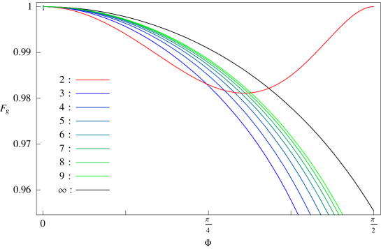
Figure 1: This figure shows the $\Phi$-dependence of the global fidelity $F_{g}$ with varying $N$ for the optimal state-dependent cloning machine. When $N=2$, $F_{g}$ approaches one at $\Phi\approx 0$ and $\Phi\approx\pi/2$. This reflects on the fact that the parallel and perpendicular quantum states can be cloned perfectly without violation of the no-cloning theorem. When $N\geq 3$, $F_{g}$ with fixed $\Phi$ increases with increasing $N$. This fact is contrary to common sense. This figure strongly suggests that the factor ‘denseness’ of the possible input states plays an important role in determining the quality of the quantum cloning process.

Now, imagine the situation, where all states in ${\cal S}_{N}$ lie between two vectors. Let the angle between these two vectors be $\Phi$. Then, we have to rescale $\theta$ as $\Phi/(N-1)$. The $\Phi$-dependence of optimal $F_{g}$ is plotted in Fig. 1. The global fidelity for the $N=2$ case (red line) is in strong agreement with Ref.bruss-98-1 . The global fidelity for $N=2$ approaches one when $\Phi\approx 0$ and $\Phi\approx\pi/2$. This reflects on the fact that two parallel or perpendicular states can be perfectly copied without violation of the no-cloning theoremwootters82 . Thus, the no-cloning theorem plays a crucial role in determining the quality of the clones when $N=2$. As Fig. 1 has exhibited, the no-cloning theorem does not play an important role when $N\geq 3$. In these cases the quality measure $F_{g}$ shows a decreasing behavior with increasing $\Phi$. However, a surprising result is the fact that $F_{g}$ with fixed $\Phi$ becomes larger and larger with increasing $N$ and eventually approaches the limiting value corresponding to $N=\infty$ (black line in Fig. 1).

The limiting value can be computed by considering the continuum case as follows. Let the input state be one of $\lvert\psi(x)\rangle=\cos x\lvert 0\rangle+\sin x\lvert 1\rangle$, where $-\Phi/2\leq x\leq\Phi/2$. Then, one can define a unitary transformation for two states out of $\lvert\psi(x)\rangle$ in a similar way. The global fidelity for this continuum case can be defined as a mean value

$$F_{g}=\frac{1}{\Phi}\int_{-\Phi/2}^{\Phi/2}dx|\langle\psi(x)\rvert\langle\psi(x)\rvert U\lvert\psi(x)\rangle\lvert\;\;\rangle|^{2}.$$

Then, applying the Lagrange multiplier method to this case and manipulating the constraints and extrema equations similarly, one can compute the optimal $F_{g}$ numerically, which is the black line in Fig. 1.

The increasing behavior of the global fidelity with increasing $N$ in fixed $\Phi$ is contrary to common sense if a priori information is measured in terms of the Shannon entropy. Instead, the ‘denseness’ of the states determines the quality of the cloning output. Although the calculational results of other quality measures are not explicitly presented in this article, one can show that they exhibit similar behaviors. As far as we know, this is a completely new and unknown phenomenon in the cloning process. With further research we think that this strange behavior, which we would like to call the ‘denseness’ effect, can be better understood within quantum mechanical law in the future.

- (1) M. A. Nielsen and I. L. Chuang, Quantum Computation and Quantum Information (Cambridge University Press, Cambridge, England, 2000).
- (2) C. H. Bennett and G. Brassard, Quantum Cryptography, Public Key Distribution and Coin Tossings, in Proceedings of the IEEE International Confer ence on Computer, Systems, and Signal Processing, Bangalore, India (IEEE, New York, 1984 ), pp. 175-179.
- (3) A. K. Ekert, Quantum Cryptography Based on Bell’s Theorem, Phys. Rev. Lett. 67 (1991) 661.
- (4) R. Alléaume et al, SECOQC white paper on Quantum Key Distribution and Cryptography [quant-ph/0701168].
- (5) S. Ghernaouti-Hélie et al, , SECOQC Business White Paper [arXiv:0904.4073 (quant-ph)].
- (6) R. P. Feynman, Simulating Physics with Computers, Int. J. Theor. Phys. 21 (1982) 467.
- (7) R. P. Feynman, Quantum Mechanical Computers, Found. Phys. 16 (1986) 507.
- (8) T. D. Ladd, F. Jelezko, R. Laflamme, Y. Nakamura, C. Monroe, and J. L. O’Brien, Quantum computers, Nature, 464 (2010) 45.
- (9) W. K. Wootters and W. H. Zurek, A single quantum cannot be cloned, Nature, 299 (1982) 802.
- (10) V. Buzek and M. Hillery, Quantum copying: Beyond the no-cloning theorem, Phys. Rev. A54 (1996) 1844 [quant-ph/9607018].
- (11) D. Bruß, D. P. Divincenzo, A. Ekert, C. A. Fuchs, C. Macchiavello, and J. A. Smolin, Optimal universal and state-dependent quantum cloning, Phys. Rev. A57 (1998) 2368 [quant-ph/9705038].
- (12) P. Zanardi, Quantum cloning in dimensions, Phys. Rev. A58 (1998) 3484 [quant-ph/9804011].
- (13) R. F. Werner, Optimal cloning of pure states, Phys. Rev. A58 (1998) 1827 [quant-ph/9804001].
- (14) M. Keyl and R. F. Werner, Optimal cloning of pure states, testing single clones, J. Math. Phys. 40 (1999) 3283 [quant-ph/9807010].
- (15) N. Gisin and S. Massar, Optimal Quantum Cloning Machines, Phys. Rev. Lett. 79 (1997) 2153 [quant-ph/9705046].
- (16) N. J. Cerf, Pauli Cloning of a Quantum Bit, Phys. Rev. Lett. 84 (2000) 4497 [quant-ph/9803058].
- (17) C. S. Niu and R. B. Griffiths, Optimal copying of one quantum bit, Phys. Rev. A58 (1998) 4377 [quant-ph/9805073].
- (18) G. Vidal, Efficient classical simulation of slightly entangled quantum computations, Phys. Rev. Lett. 91 (2003) 147902 [quant-ph/0301063].
- (19) R. Jozsa and N.Linden, On the role of entanglement in quantum computational speed-up, Proc. R. Soc. Lond. A 459, (2003) 2011 [quant- ph/0201143].
- (20) P. Masiak, Entanglement preservation in quantum cloning, J. Mod. Opts. 50 (2003) 1873 [quant-ph/0309019].
- (21) J. Novotny, G. Alber, and I. Jex, Optimal copying of entangled two-qubit states, Phys. Rev. A71 (2005) 042332 [quant-ph/0411105].
- (22) E. Karpov, P. Navez, and N. J. Cerf, Cloning quantum entanglement in arbitrary dimensions, Phys. Rev. A72 (2005) 042314 [quant-ph/0503148].
- (23) S. K. Choudhary, S. Kunkri, R. Rahaman, and A. Roy, it Local cloning of entangled qubits, Phys. Rev. A76 (2007) 052305, arXiv:0706.2459 (quant-ph).