Quantum state tomography of an itinerant squeezed microwave field

Abstract

We perform state tomography of an itinerant squeezed state of the microwave field prepared by a Josephson parametric amplifier (JPA). We use a second JPA as a pre-amplifier to improve the quantum efficiency of the field quadrature measurement (QM) from 2 % to $36\pm 4~{}\%$. Without correcting for the detection inefficiency we observe a minimum quadrature variance which is $68^{+9}_{-7}~{}\%$ of the variance of the vacuum. We reconstruct the state’s density matrix by a maximum likelihood method and infer that the squeezed state has a minimum variance less than 40 % of the vacuum, with uncertainty mostly caused by calibration systematics.

Fundamental quantum optics experiments at microwave frequencies have been recently performed with superconducting qubits or Rydberg atoms inside high-quality microwave cavities. Examples include the reconstruction of the Wigner functions of Fock states from one Houck et al. (2007) to a few photons and coherent superpositions of few photons Deléglise et al. (2008); Hofheinz et al. (2008, 2009). States such as these, which are manifestly nonclassical light states, are crucial for quantum information processing, because they can be used to generate entanglement. However, in the cited experiments, these states are confined in cavities. Therefore distributing entanglement to separate parties, as required in quantum communication protocols, remains challenging for microwave implementations. In contrast to the discrete Fock state approach, continuous variables quantum information (CVQI) strategy uses another type of nonclassical states, the squeezed states, which are readily created in itinerant modes. These states exhibit reduced noise, below the vacuum fluctuations, in one of their quadrature components and amplified noise in the other one. They are also easily generated at optical frequencies in the itinerant output modes of parametric amplifiers made of optically nonlinear crystals. At optical frequencies, CVQI has progressed rapidly from the initial creation of squeezed states Slusher et al. (1985) and tomographic reconstruction Smithey et al. (1993); Schiller et al. (1996); Breitenbach et al. (1997) of those states to teleportation Furusawa et al. (1998); Yonezawa et al. (2007) and quantum error correction Aoki et al. (2009); Lassen et al. (2010).

At microwave frequencies, the field is less advanced. The generation of microwave squeezed states using the nonlinear electrical response of superconducting Josephson junctions has been reported Yurke et al. (1988), with inferred squeezing down to $10~{}\%$ of vacuum variance Castellanos-Beltran et al. (2008). Such states can be powerful tools for quantum information processing and communication because microwaves and superconducting qubits can mimic useful light–atom interactions, as demonstrated in Wallraff et al. (2004). Furthermore, these devices are made of compact and integrable electrical circuits, with much promise for building complex quantum information processors. The lack of an efficient quadrature measurement (QM) for itinerant modes has slowed the advancement of CVQI. However, as demonstrated recently in Teufel et al. (2009), it is possible with a JPA to realize an efficient single QM.

In this Letter, we report the tomography of an itinerant squeezed microwave field. We demonstrate that our JPA based measurement scheme has a quantum efficiency $20$ times greater than a QM employing state-of-art semiconductor amplifiers. We infer the quantum state prepared by maximum likelihood tomography, correcting for inefficiency in our QM. We discuss the achieved degree of squeezing, from the perspective of generating entanglement on chip.

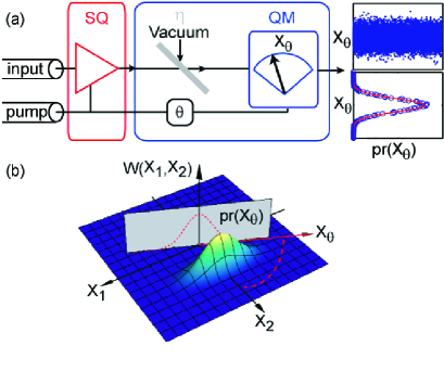
Homodyne tomography is a standard experimental tool to infer the quantum state of a single mode of light. It was proposed in Vogel and Risken (1989) and pioneered on a squeezed optical field in Smithey et al. (1993). Its principle is depicted in the Fig. 1. A homodyne detection apparatus measures the value of the quadrature $X_{\theta}$, where $\theta$ is set by adjusting the phase of the local oscillator. The probability density function $\textrm{pr}(X_{\theta})$ for measuring a particular value of $X_{\theta}$ is the marginal density function of the Wigner function, i.e. $\textrm{pr}(X_{\theta})=\int dX_{\theta+\pi/2}W(X_{\theta},X_{\theta+\pi/2})$, as shown in Fig. 1 (b). Thus by performing measurements of $X_{\theta}$ on many identical copies of the state and varying $\theta$, the “hidden” quantum object can be seen from different angles and its state inferred. Losses and other Gaussian noise sources in the homodyne detector can be modeled with the insertion of a fictitious beam splitter of transmissivity $\eta$, as shown in Fig. 1 (a). In such a case, the measured $\textrm{pr}(X_{\theta})$ are no longer the projections of the desired Wigner function $W$, but of a smoother distribution which is the convolution of $W$ with a Gaussian Wigner function Leonhardt and Paul (1993). However methods like maximum likelihood quantum state tomography can be used to deconvolve the effect of inefficiency Lvovsky and Raymer (2009).

Figure 1: Principle of the experiment.  (a-left): The squeezer (SQ, in red) prepares a squeezed state whose quadrature distributions are measured for different phases $\theta$ with an efficiency $\eta$.  (a-right): Simulated measurement results for 20,000 realizations of creating the squeezed state and measuring it at a single $\theta$. The top graph shows the measured quadrature value versus realization number. The bottom plot is a histogram (blue circles) and Gaussian probability distribution $\textrm{pr}(X_{\theta})$ (red curve) of this random process.  (b): Graphical Interpretation: the probability distribution $\textrm{pr}(X_{\theta})$ is simply the projection of the Wigner function.

At optical frequencies, $\eta\geq 90~{}\%$ is routinely obtained using a pair of balanced photodiodes Lvovsky and Raymer (2009). Such detectors are not available for microwaves and until recently the best setup was a chain of phase-insensitive amplifiers followed by a mixer, or two such chains in parallel Menzel et al. (2010); Mariantoni et al. (2010); Bozyigit et al. (2010). In such a case, noise $A_{n}$ greater than $1/2$ (the vacuum variance) must be added to the QM Caves (1982). This noise can be modeled as an effective efficiency by the relation $\eta=1/(1+2A_{n})$ Leonhardt and Paul (1994), so the QM efficiency using phase-insensitive amplifiers is limited to $50~{}\%$. State of the art microwave amplifiers, high-electron-mobility transistors (HEMTs), have $A_{n}\approx 10-20$. In practice, the unavoidable losses present in a microwave experiment typically result in $\eta\approx 2$%. However, as demonstrated in Teufel et al. (2009), inserting a JPA used as a single quadrature preamplifier before the HEMT increases the experimentally achieved $\eta$ by a factor of approximately 20.

To perform a high-quality reconstruction of the Wigner function of a squeezed microwave state we operate two JPAs in series, as shown in Fig. 2 (b). The first JPA, referred to as the squeezer (SQ), prepares the squeezed state. The second JPA, referred to as the pre-amplifier (AMP), amplifies the quadrature of the squeezed state determined by the phase difference $\theta$ between the AMP and the SQ pump tones. We vary $\theta$ by applying to the two cavities pump tones slightly detuned from one another. The SQ stage is pumped at $7.45$ GHz, while the AMP stage is pumped at $100$ kHz higher frequency; therefore, sweeping $\theta$ through $2\pi$ every $10$ µs.

Our implementation of an SQ or an AMP at microwaves, as shown in Fig. 2 (a), requires three elements: (i) a JPA used in reflection, (ii) a directional coupler and (iii) a circulator. As described in Castellanos-Beltran et al. (2008), the JPAs are nonlinear resonant cavities built from coplanar waveguides whose central conductor has been replaced by a series of many Josephson junctions. The Josephson junctions’ nonlinearity causes the cavity’s phase velocity to be intensity dependent. Therefore when the cavity is pumped it becomes a phase sensitive amplifier for input modes whose frequencies lie within the bandwidth of the JPA centered on the pump frequency. Such microwave modes incident on the JPA are reflected and exit the cavity with one quadrature amplified and the other squeezed, depending on their phase relative to the pump’s phase. A directional coupler is used to add the pump tone to the incident signal and remove the pump tone from the reflected signal. Finally the incident and reflected modes are separated into different cables using a circulator.

Figure 2:  (a): To implement a SQ or AMP at microwaves, three microwaves components are required: (i) a JPA, (ii) a directional coupler and (iii) a circulator. Taking port (1) of the directional coupler as reference, (2) is the weakly coupled port, (3) the isolated port and (4) the direct port. Port (2) is used to pump the JPA. Port (3) is used to apply a cancelation tone (adjusted with a room temperature attenuator and phase shifter) that nulls the pump and displaces the output of the JPA back to the origin of the phase space. (b): Schematic of the experiment. In this figure, all the microwave components and cables are considered lossless; their imperfections are absorbed into the experimentally determined total transmissivities $\xi$, $\alpha$ and $\beta$.

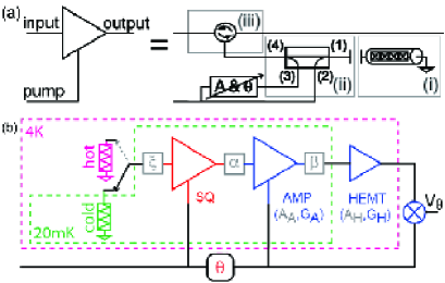
Following Fig. 2 (b), in the limit of large HEMT power gain $G_{H}$, our quantum efficiency can be cast as

$$\eta=\frac{\alpha}{2+2A_{A}-\alpha+[2A_{H}-(1-\beta)]/G_{A}\beta},$$ (1)

where $A_{A}$ ($A_{H}$) is the AMP (HEMT) added noise, $\alpha$ ($\beta$) is the fraction of power transmitted by the microwave circuitry between the SQ and the AMP (the AMP and the HEMT), and $G_{A}$ is the power gain of the AMP stage. A detailed description of how we calibrate each of these parameters is in the supplementary information. Briefly, we inject different amounts of thermal noise into the amplifier chain while operating each JPA either as an amplifier (ON) or as a noiseless element with unit gain (OFF). We then infer the added noise and loss of the elements by observing the variation in the noise at the output of the measurement chain. The thermal noise is varied by connecting the input of the SQ through a switch to either a “hot load” (50 $\Omega$ microwave termination at $4.1$ K) or a “cold load” (at $20$ mK). Although the tomography is only performed with the “cold load”, both are required for calibration. We obtain $A_{A}=0.25\pm 0.06$, $A_{H}=17.3\pm 0.1$, $\alpha=68\pm 2~{}\%$ and $\beta=74\pm 5~{}\%$. However, as the switch is operated at the 4.1 K stage and is slightly lossy, the state presented at the input of the SQ with the “cold load” is not pure quantum vacuum, but a low occupancy thermal state with average photon number $\overline{n}\simeq 0.15\pm 0.15$. One quadrature of the resulting squeezed state is then amplified at the AMP stage with sufficient gain $G_{A}=180$ such that the noise in the amplified quadrature exceeds $A_{H}$ for any $\theta$. From Eq. (1), we obtained an overall quantum efficiency of $36\pm 4~{}\%$, which can be compared to $\eta\approx 2~{}\%$ without the AMP stage.

In this experiment our uncertainty in $\eta$ and $\overline{n}$ create a systematic source of error. We thus perform our data analysis under three assumptions (1) high efficiency ($\eta=0.40$) and high mean photon number ($\overline{n}=0.30$), (2) best estimate for both efficiency ($\eta=0.36$) and mean photon number ($\overline{n}=0.15$), and (3) low efficiency ($\eta=0.33$) and low mean photon number ($\overline{n}=0$). These three cases give us “pessimistic”, “best-guess”, and “optimistic” analyses, in terms of the purity of the squeezed state estimated by the tomography. Using a lower estimate for $\eta$ and $\overline{n}$ as inputs to the tomography algorithm causes it to return a more pure, more squeezed, and therefore a more “optimistic” estimate of the squeezed state. Associated with each of these three cases, we also have statistical uncertainty, so the given error bounds cover an interval that includes both uncertainties around the “best-guess” estimate. They are reported in the form $X_{-L}^{+U}$, where $X$ is the statistical mean using the “best-guess” calibration and $L$ and $U$ are respectively the lower and upper bounds of the one standard deviation uncertainty in the “pessimistic” and “optimistic” cases.

We must also calibrate the QM to convert the measured voltage noise into units of noise quanta. In optical homodyne tomography, this is usually done by inserting the vacuum and observing the quadrature noise. Analogously, we insert the weak thermal state with mean photons $\overline{n}$ (by simply turning the SQ stage OFF) and measure voltages proportional to quadrature values at many $\theta$, as shown (in blue) in Fig. 3. As expected this voltage noise is $\theta$ independent, with a variance $\Delta V_{\mathrm{SQ,OFF}}^{2}=3.2\times 10^{-5}~{}\textrm{mV}^{2}$. Under the convention that vacuum has variance $1/2$ in unitless quadrature space (or in units of “quanta”), we calibrate this voltage variance to $\Delta X_{\mathrm{SQ,OFF}}^{2}=(1-\eta)/2+\eta(1/2+\overline{n})=0.55_{-0.05}^{+0.07}$ quanta. Therefore the desired conversion factor $\Delta X_{\mathrm{SQ,OFF}}^{2}/\Delta V_{\mathrm{SQ,OFF}}^{2}=1.71_{-0.17}^{+0.20}\times 10^{4}~{}\mathrm{quanta/mV}^{-2}$ is used to rescale the variances in Fig. 3 (c).

Figure 3:  (a): Density plot of number of occurrences in a $1~{}$µV bin size of the amplified quadrature voltage $V_{\theta}$ versus $\theta/2\pi$, with the SQ pump OFF (top) and ON (bottom). (b): In particular, histograms of $V_{\theta}$ at the maximum of squeezing: data ($\circ$) and Gaussian fit (continuous lines) for the SQ pump OFF (blue) and ON (red). (c): Noise variance $\Delta X^{2}_{\theta}$ in quanta units on a log scale versus $\theta/2\pi$ for the SQ pump ON (red) and OFF (blue). The (black) line indicates our estimate of the vacuum noise level under the “best-guess” calibration.

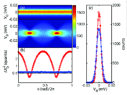
In Fig. 3 (a), we show QM data of the squeezed state. With SQ ON (red) we observe the characteristic phase dependent noise for a squeezed state. At the phase for which the variance is minimum, we show the histogram of quadrature measurements in Fig. 3 (b). The SQ OFF histogram is clearly wider than the SQ ON histogram, demonstrating our ability to observe squeezing directly at the output of our measurement chain. In Fig. 3 (c) we plot the variance of the QM with SQ ON and OFF as a function of $\theta$, expressed in units of quanta, clearly showing squeezing below the vacuum level. Without correcting for $\eta$, we observe a minimum quadrature variance which is $\Delta X^{2}_{\mathrm{SQ,MIN}}=68_{-7}^{+9}~{}\%$ of the vacuum variance.

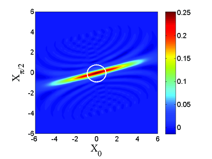
To infer the quantum state created by the squeezer, correcting for loss during the QM, we used maximum likelihood quantum state tomography Hradil et al. (2004). For each of the three calibration cases, we performed 35 reconstructions using independent subsets each containing 10,000 QMs of the total measured data. We estimated statistical uncertainty from the spread of properties (such as fidelity or minimum variance) of the set of 35 reconstructions. The statistical uncertainty was significantly lower than the systematic uncertainty. In Fig. 4 we show the Wigner function of the “best-guess” reconstructed state $\rho$. The pure squeezed vacuum state $|\psi\rangle$ that has the highest fidelity with $\rho$ has minimum quadrature variance $6.0_{-1.1}^{+1.4}~{}\%$ of the vacuum variance, and that maximum fidelity is $F=\langle\psi|\rho|\psi\rangle=0.81_{-0.17}^{+0.16}$. As explained in the supplementary information, the minimum variance of $\rho$ is biased by an amount comparable to our systematic uncertainty, so we infer the minimum variance $\Delta x^{2}_{\mathrm{SQ,MIN}}$ directly from the observed minimum variance as $\Delta x^{2}_{\mathrm{SQ,MIN}}=(1/\eta)(\Delta X^{2}_{\mathrm{SQ,MIN}}-(1-\eta)/2)$. We find $\Delta x^{2}_{\mathrm{SQ,MIN}}=12^{+30}_{-12}~{}\%$ of the vacuum variance. For comparison, the most highly squeezed optical state ever made has a variance of only $7~{}\%$ of the vacuum variance Mehmet et al. (2010).

Figure 4: Mean of 35 reconstructions of the Wigner function of the state exiting the SQ, inferred by maximum likelihood under the “best-guess” assumption, in quanta units. The faint pattern of ripples extending from the origin is caused by truncation at 30 photons of the density matrix used to represent the state. The white circle at the origin shows the full-width at half-maximum of the vacuum state.

Producing squeezed states of itinerant modes allows the generation of distributable entanglement by sending two copies of a squeezed vacuum state through the two input ports of a balanced beam splitter. The coherent information Schumacher and Nielsen (1996) is one useful way to characterize the entanglement between the two output modes. The asymptotic number of maximally entangled qubit pairs (e-bits) that can be distilled per copy of the noisy entangled state, by using local operations and one-way classical communication, is at least as large as the coherent information Devetak and Winter (2005). Given two copies of $\rho$, one could make two entangled modes with $2.5^{+1.0}_{-0.4}$ e-bits of coherent information.

In conclusion, we have reconstructed the Wigner function of an itinerant squeezed microwave field generated at the output of a Josephson Parametric Amplifier. Using a second JPA as a preamplifier has increased the quantum efficiency of the microwave homodyne detection from approximately $2~{}\%$ to $36~{}\%$. The level of squeezing is primarily limited by noise added to the squeezed state by the JPA. Improving the performance of the JPAs (as both squeezers and phase-sensitive amplifiers) will require more detailed investigation of the source of this noise. We used maximum likelihood quantum state tomography to deconvolve the QM inefficiency in order to precisely characterize the state generated. This is an important step toward generating easily distributable microwave entanglement on chip.

Notes: A different method was recently used to obtain a similar state reconstruction Eichler et al. (2010).

I Supplementary Materials for “Quantum state tomography of an itinerant squeezed microwave field”

II Data acquisition and calibration

Determining the amplifier added noise and loss requires several calibration steps that permit us to isolate the effect of a specific loss or added-noise contribution to the overall efficiency of the homodyne measurement. The crucial aspect that makes this calibration possible is that the JPA cavities have widely-tunable resonance frequencies, adjusted by imposing a magnetic flux Castellanos-Beltran et al. (2008, 2009). Far from resonance the JPA cavities behave as open circuits. They are simply mirrors that reflect the microwave field without otherwise transforming it; therefore, either the SQ or AMP or both stages can effectively be bypassed.

We begin with both JPA stages bypassed, so that they have $G_{\rm{S}}=G_{\rm{A}}=1$. If the switch were lossless, when it is connected to the cold load, the noise power exiting the HEMT amplifier would be $S=G_{H}(A_{H}+S_{f})$, where $S_{f}=(1/2)+n_{f}=(1/2)+[\exp(\hbar\omega/k_{B}T_{f})-1]^{-1}$ and $T_{f}$ is the refrigerator’s temperature. Notice that the result doesn’t depend on the transmissivities $\alpha$, $\beta$, or $\xi$ because these are at the same temperature as the cold load, consequently each loss component emits as much power as it absorbs. However, with the switch connected to the hot load, the expression for the total power at the output becomes $S=G_{H}(A_{H}+(\xi\alpha\beta)S_{h}+(1-\xi\alpha\beta)S_{f})$, with $S_{h}=(1/2)+n_{h}=(1/2)+[\exp(\hbar\omega/k_{B}T_{h})-1]^{-1}$ and $T_{h}=4.1$ K. In both cases, we expect and observe that $S$ depends linearly on $S_{f}$ with an offset. By fitting these linear dependencies we can extract $G_{H}$, $A_{H}$, and the product $\xi\alpha\beta$.

We cannot assume that the switch is lossless. Because its loss sits at 4.1 K, it will always emit noise power $S_{h}(1-\lambda)+S_{in}\lambda$, where $S_{in}$ is the incident noise and $\lambda$ is the switch transmissivity. So, even when $n_{f}\ll 1/2$, the state presented at the SQ stage will have average thermal occupancy $\bar{n}=(1-\lambda)\xi n_{h}$. We write the noise power at the output as function of $S_{f}$, for switches in both positions as

$$S_{1c}=G_{H}A_{H}+S_{h}G_{H}(1-\lambda)\xi\alpha\beta+S_{f}[G_{H}\lambda\xi\alpha\beta+G_{H}(1-\xi\alpha\beta)]=b_{1c}+m_{1c}S_{f}$$ (2)

$$S_{1h}=G_{H}A_{H}+S_{h}G_{H}(\xi\alpha\beta)+S_{f}[G_{H}(1-\xi\alpha\beta)]=b_{1h}+m_{1h}S_{f},$$ (3)

where the subscript $1c$ ($1h$) corresponds to the switch connected to the cold (hot) load. Fitting our noise data to the right hand side of Eq. 2 and 3, we can obtain the four parameters $b_{1h},b_{1c},m_{1h}$ and $m_{1c}$. However as these parameters are not independent, $S_{h}=(b_{1h}-b_{1c})/(m_{1c}-m_{1h})$, we cannot extract the switch loss independently. We can nevertheless bound this unknown loss by taking a worst case estimate as the manufacturers minimum specified transmission (at room temperature) $\lambda=0.83$ and assuming it is less lossy at 4.1 K. We moreover confirmed that at room temperature the frequency dependent loss of the switch is within the manufacturer’s specification. Then by using $1<\lambda<0.83$, we can bound the desired parameters using Eq. 2 and 3, with the expressions $(\xi\alpha\beta)^{-1}=1+m_{1h}S_{h}\lambda/(b_{1h}-b_{1c})$, and $G_{H}=m_{1h}/(1-\xi\alpha\beta)$, and $A_{H}=(b{1c}/G_{H})-(1-\lambda)S_{h}(\xi\alpha\beta)$.

We then perform the same analysis, finding the linear dependence of the output noise on $S_{f}$ and on the switch position, with the AMP ON and SQ OFF. From these fits and knowledge of $A_{H}$ and $G_{H}$ we find $\xi\alpha$, $A_{A}$, and$G_{A}\beta$. Finally, we operate the experiment with AMP OFF and SQ ON. A third time we fit the linear dependence of $S$ on $S_{f}$ with the switch in both positions, determining $\xi$, $\alpha$ and $\beta$ separately (Fig. 5b). We evaluate the expressions for $\alpha$, $\beta$, $A_{A}$, $A_{H}$, $G_{H}$ and $\bar{n}$ at the bounds on $\lambda$, finding the range of values in the main text. We also find $\xi=-9.9\pm 1$ dB, of which 6 dB arises from an attenuator that has been placed at the input of the SQ stage.

Figure 5: The noise density $S$ in arbitrary units at the output of the measurement versus refrigerator temperature $T_{f}$. a.) Data acquired with the AMP and SQ OFF and the switch connected to the cold load (circles) and hot load (squares). The lines are linear fits to $S$ versus $S_{f}$ for the case of the switch connected to the cold load (solid) and hot load (dashed). b.) Data acquired with the AMP ON and SQ OFF (blue) and AMP OFF and SQ ON (red), with the switch connected to the cold load (circles) with a linear fit (solid) and hot load (squares) with a linear fit (dashed). The arbitrary y-scale is consistent between the six plots. The linear fits do not appear as lines because we plot $S$ versus $T_{f}$ rather than $S_{f}$.

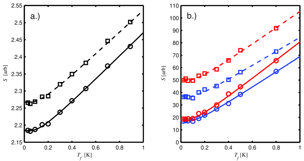
To acquire these calibration data sets, we regulate the refrigerator’s temperature at 10 values between base temperature ($T<50$ mK) and 800 mK, which requires about 7 hours to complete. For each temperature point we measure the noise at the output under all six conditions, 2 switch positions, and 3 amplifier configurations (AMP OFF SQ OFF, AMP ON SQ OFF, and AMP OFF SQ ON). We inject a tone detuned from the AMP pump by 20 kHz. By dividing the noise power at the output of the chain by the power in this tone, we become insensitive to any variation in $G_{H}$ over the time needed to acquire the data. At the end of the calibration, we immediately operate the experiment with SQ ON and AMP ON, to acquire the data in the paper. In addition, we use the tone to ensure that we do not saturate the amplifier chain.

Data is acquired by digitizing the output (IF port) of the mixer at rate of $10^{7}$ samples per second. We filter the IF port with a 5 MHz anti-aliasing low-pass filter. The digitized data is digitally filtered with a 3rd-order Butterworth high-pass filter with a 500 kHz corner (3 dB) frequency. The noise density $S$ is the average noise density in the frequency range between 500 kHz and 5 MHz.

III Maximum likelihood analysis of the squeezed state

Table 1: Inferred properties of the squeezed state, upon our three analysis assumptions.

	Pessimistic	Best guess	Optimistic
Fidelity	$0.66\pm 0.02$	$0.807\pm 0.016$	$0.960\pm 0.005$
Min. var. of comparison pure state $\left|\psi\right\rangle$:
	$0.065\pm 0.009$	$0.060\pm 0.003$	$0.0493\pm 0.0006$
$\rho$’s purity	$0.62\pm 0.02$	$0.74\pm 0.02$	$0.96\pm 0.01$
$\rho$’s sq. var.	$0.918\pm 0.002$	$0.484\pm 0.013$	$0.304\pm 0.008$
$\rho$’s anti-sq. var.	$25.54\pm 0.07$	$20.17\pm 0.06$	$19.18\pm 0.05$
Coherent info.	$2.19\pm 0.08$	$2.46\pm 0.09$	$3.42\pm 0.05$
Linear sq. var.	$0.40\pm 0.02$	$0.12\pm 0.02$	$-0.18\pm 0.02$

Table 1 shows the statistical errors in our estimates of inferred parameters characterizing the squeezed state, for the three analysis cases, based upon our systematic calibration uncertainties. The first line presents the fidelity $F=\langle\psi|\rho|\psi\rangle$, where $\rho$ is the maximum likelihood reconstructed density matrix of the field exiting the SQ and $|\psi\rangle$ is the pure vacuum squeezed state that maximizes the fidelity. The second line gives the ratio of the minimum variance of $|\psi\rangle$ to the variance of vacuum. The third line gives the purity $\mathrm{Tr}({\rho^{2}})$ of $\rho.$ The fourth and fifth lines give the ratios of the squeezed and anti-squeezed variances of the reconstructed state to the variance of vacuum. The sixth line presents the coherent information that could be obtained by combining on a beam splitter two copies $\rho$. The last line gives our estimate the the experimental states’ minimum variance based on direct linear inference.

We have stated three variances that characterize the state created in this experiment: the linear estimate of the experimental state’s minimum variance ($12~{}\%$), the most likely state $\rho$’s minimum variance ($48~{}\%$), and the minimum variance of the pure squeezed vacuum state $\left|\psi\right\rangle$ that maximizes the fidelity with $\rho$ ($6.0~{}\%$). Here we give more discussion of these variances.

The quadrature measurements we observe are the linear combination of the quantum state created by the squeezer and vacuum fluctuations:

$$X_{\theta}=\sqrt{\eta}x_{\theta}+\sqrt{(1-\eta)}y_{\theta},$$

where $x_{\theta}$ is the quadrature of the squeezed state, and $y_{\theta}$ is the quadrature of the vacuum state. Solving for $x_{\theta}$ gives

$$x_{\theta}=\frac{1}{\sqrt{\eta}}\left(X_{\theta}-\sqrt{\left(1-\eta\right)}y_{\theta}\right).$$

Therefore the inferred variance of the squeezed state’s quadrature $\Delta x_{\theta}^{2}$ is

$$\Delta x_{\theta}^{2}=\frac{1}{\eta}\left[\Delta X_{\theta}^{2}-\left(1-\eta\right)\Delta y_{\theta}^{2})\right].$$

The vacuum variance $\Delta y_{\theta}^{2}=1/2$, and we can easily calculate an unbiased estimate of $\Delta X_{\theta}^{2}$ for every phase $\theta$. This gives us an unbiased estimate of $\Delta x_{\theta}^{2}$ that does not depend on the details (for example, Gaussianity) of the quantum state. We calculate $\Delta x_{\theta}^{2}$ using 20,000 quadrature measurements at each of 100 evenly spaced $\theta$ and calculate the minimum value $\Delta x_{\mathrm{SQ,MIN}}^{2}$, in Table 1. The statistical uncertainties show one standard deviation in the estimate of $\Delta x_{\mathrm{SQ,MIN}}^{2}$. For the “optimistic case” we calculate a negative variance, which is clearly unphysical. This is a sign of inconsistency in the “optimistic” calibration parameters. Because the “optimistic” estimate for the squeezed state is computed using the lower bounds on $\eta$ and $\overline{n}$, this negative variance is evidence that the detector’s true $\eta$ and / or effective gain ($\Delta X_{\mathrm{SQ,OFF}}^{2}/\Delta V_{\mathrm{SQ,OFF}}^{2}$) must be larger than the lower bounds set by calibration.

The minimum variance of $\rho$ is significantly higher than this linear estimate. This is caused by bias in the maximum likelihood method. Quantum state estimation by maximum likelihood is biased toward more mixed states, and the amount of bias increases with increasing purity of the state from which the measurements are drawn Glancy et al. (2009). Based on numerical experiments, the bias in our estimates of the fidelity should be well below the uncertainty level set by systematic effects. However, the bias in our estimates of the minimum variance of the inferred state could be larger. To attempt to quantify this effect, we simulated measuring and performing maximum likelihood tomography on a Gaussian state. This Gaussian state is chosen to have minimum and maximum variances equal to those calculated by the linear method described above for the “best-guess” case. By computer we simulate 10,000 quadrature measurements (the same number we used for ML analysis of the true experiment) from this Gaussian state and perform maximum likelihood tomography on those measurements. The inferred state has minimum variance $40~{}\%$. Therefore it is possible that the experimental state has smaller minimum variance than the most likely state inferred from only 10,000 measurements. Because we have some independent evidence for non-Gaussian effects in the experiment, we cannot quantify this size of this bias using this Gaussian simulation. Other numerical simulations have confirmed that this bias decreases as the number of measurements analyzed increases and that this bias is not caused by truncation of the Hilbert space at 30 photons.

The apparent discrepancy between the $6~{}\%$ for the variance of $|\psi\rangle$ and the $48~{}\%$ for the variance of $\rho$ also deserves some comments. It is important to note that one would not expect the minimum variance of a mixed state to equal the minimum variance of its highest fidelity pure state. The fidelity between a mixed Gaussian state (centered at the origin of phase space) whose minimum and maximum variances are $v_{x}$ and $v_{p}$ and a pure squeezed vacuum state with minimum variance $v_{s}$ is given by

$$F_{\mathrm{Gauss}}=\frac{2}{\sqrt{\frac{(1+4v_{s}v_{p})(v_{s}+v_{x})}{v_{s}}}}.$$

The highest fidelity pure state has minimum variance $v_{s}=\frac{1}{2}\sqrt{\frac{v_{x}}{v_{p}}}$, and the fidelity between these two states is

$$F_{\mathrm{Gauss,max}}=\frac{2}{1+2\sqrt{v_{x}v_{p}}}$$

Consider the state $\sigma$ to be a Gaussian state with minimum variance of $48~{}\%$ and maximum variance $2017~{}\%$. ($\sigma$ has variances equal to those of our state $\rho$, but unlike $\rho$, $\sigma$ is guaranteed to be Gaussian.) Then let $|\psi\rangle$ be the pure squeezed vacuum state that has maximum fidelity with $\sigma$. $F_{\mathrm{Gauss,max}}=\langle\psi|\sigma|\psi\rangle=0.49$, and the minimum variance of $|\psi\rangle$ is $7.7~{}\%$. The difference between the minimum variances of $\rho$ and $\left|\psi\right\rangle$ is to be expected. However, the maximum fidelity of $\rho$ is significantly larger than we would expect if it was perfectly Gaussian. This non-Gaussianity could be caused by bias in the maximum likelihood inference and / or genuine non-Gaussian effects in the experiment.

Tomographic reconstruction of a quantum state requires that the experimental device always creates the same (potentially mixed) quantum state, that the measurements are well described by inefficient quadrature measurements, and that the calibration of those measurements is consistent. In this experiment we have observed some evidence that at least one of these assumptions is violated. The likelihood of the maximum likelihood state is significantly lower than one should expect from simulated measurements on that state. That is, if the tomographic assumptions above were true, we expect to find a significantly higher value for the maximum likelihood. We believe this effect could be caused by an interaction between the state preparation and measurement stages of the experiment, such as a phase dependent efficiency of the measurement JPA, and/or non linear processes in the measurement.