QCD corrections to the hadronic production of a heavy quark pair and a W𝑊W-boson including decay correlations

Simon Badger simon.badger@nbi.dk Niels Bohr International Academy and Discovery Center, The Niels Bohr Institute, Blegdamsvej 17, DK-2100 Copenhagen, Denmark    John M. Campbell johnmc@fnal.gov    R. K. Ellis ellis@fnal.gov Theoretical Physics Department, Fermi National Accelerator Laboratory,
P. O. Box 500, Batavia, IL 60510, USA
Abstract

We perform an analytic calculation of the one-loop amplitude for the W𝑊W-boson mediated process 0du¯QQ¯¯0𝑑¯𝑢𝑄¯𝑄¯0\to d\bar{u}Q\bar{Q}\bar{\ell}\ell retaining the mass for the quark Q𝑄Q. The momentum of each of the massive quarks is expressed as the sum of two massless momenta and the corresponding heavy quark spinor is expressed as a sum of two massless spinors. Using a special choice for the heavy quark spinors we obtain analytic expressions for the one-loop amplitudes which are amenable to fast numerical evaluation. The full next-to-leading order (NLO) calculation of hadron+hadronW(eν)bb¯{\rm hadron}~{}+~{}{\rm hadron}\to W(\to e\nu)b\bar{b} with massive b𝑏b-quarks is included in the program MCFM. A comparison is performed with previous published work.

pacs:
13.85.-t,14.65. Ha
preprint: FERMILAB-Pub-10-482-T

I Introduction

One of the most interesting channels currently under study at the Tevatron and the LHC is the final state containing a W𝑊W-boson and jets, where some or all of the produced jets are tagged as containing a bottom quark. Several interesting partonic processes contribute to this final state, for example,

  • W+H(bb¯)annotated𝑊𝐻absent𝑏¯𝑏W+H\,(\to b\bar{b})

  • W+Z(bb¯)annotated𝑊𝑍absent𝑏¯𝑏W+Z\,(\to b\bar{b})

  • b¯+t(W++b)annotated¯𝑏𝑡absentsuperscript𝑊𝑏\bar{b}+t\,(\to W^{+}+b)

  • t¯+t(W++b)annotated¯𝑡𝑡absentsuperscript𝑊𝑏\bar{t}+t\,(\to W^{+}+b)

A background to these processes involving heavy bosons and fermions, is the QCD and electroweak process occurring in the collision of hadrons H1subscript𝐻1H_{1} and H2subscript𝐻2H_{2},

H1+H2W+b+b¯+X.subscript𝐻1subscript𝐻2𝑊𝑏¯𝑏𝑋H_{1}+H_{2}\to W+b+\bar{b}+X\;. (1)

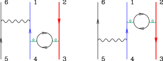
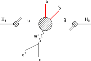
An example of a partonic subprocess contributing to this process is shown in Fig. 1. Next-to-leading corrections to this process were first considered in Ellis:1998fv , working in the approximation in which the b𝑏b-quark is considered massless. Since in many analyses the b𝑏b-quark is required to have a minimum pTsubscript𝑝𝑇p_{T}, typically 151515 GeV or more, in order to be efficiently tagged, the neglect of the mass of the bottom quark is expected to be a good approximation.
Refer to caption
Figure 1: Example of a partonic process contributing to Wbb¯𝑊𝑏¯𝑏Wb\bar{b} production

After these initial studies, this same process was considered in refs. Febres Cordero:2006sj ; Cordero:2009kv ; Cordero:2010qn ; Campbell:2008hh , without making the approximation mb=0subscript𝑚𝑏0m_{b}=0. These studies, performed without the inclusion of decay products of the W𝑊W boson effectively confirmed that the mb=0subscript𝑚𝑏0m_{b}=0 approximation is good to a few percent, with the difference parametrically suppressed as mb2/pT2superscriptsubscript𝑚𝑏2superscriptsubscript𝑝𝑇2m_{b}^{2}/p_{T}^{2}. Thus retaining the mass of the b𝑏b-quark extends the prediction to lower values of pTsubscript𝑝𝑇p_{T}. In addition, it allows us treat the case where the two b𝑏b-quarks end up in the same jet and the case when one b𝑏b-quark is either too soft or too forward to be tagged. These kinematic configurations can be important for the Higgs search at the Tevatron and the LHC :2010ar ; Butterworth:2008iy .

The purpose of this paper is to repeat the calculation of ref. Febres Cordero:2006sj , i.e. including the effects of a finite b𝑏b-quark mass, but also including the spin correlations present in the W𝑊W-boson decay. The calculation is performed using the spinor helicity formalism, with the calculated amplitudes represented as analytic formulae. Although the formulae are not compact enough to be presented in their entirety here, they do lead to an efficient and numerically stable code.

Following a four-dimensional unitarity based approach Bern:1994zx ; Bern:1994cg , we will construct the logarithmic parts of the virtual amplitude using multiple cuts. Developments to this technique utilizing complex momenta Britto:2004nc ; Britto:2005ha ; Britto:2006sj ; Forde:2007mi allow us to compute analytic expressions for the coefficients of the known scalar integrals.

The bulk of our paper is dedicated to a description of the calculation of the one-loop corrections to the process 0du¯QQ¯¯0𝑑¯𝑢𝑄¯𝑄¯0\to d\bar{u}Q\bar{Q}\bar{\ell}\ell retaining the mass for the quark Q𝑄Q. The detailed plan of this paper is as follows. In section II we present our method for dealing with massive spinors using spinor helicity techniques. Section III gives a precise definition of the amplitude that we wish to calculate, including the decomposition into colour stripped amplitudes and the further decomposition into one-loop primitive amplitudes. Sections IV, V and VI illustrate our calculation of the leading colour primitive amplitude, A6lcsubscriptsuperscript𝐴𝑙𝑐6A^{lc}_{6}, of the sub-leading colour primitive, A6slsubscriptsuperscript𝐴sl6A^{\rm sl}_{6}, and of the primitive amplitudes containing a closed loop of fermions, A6lfsubscriptsuperscript𝐴lf6A^{\rm lf}_{6} and A6hfsubscriptsuperscript𝐴hf6A^{\rm hf}_{6}. Section VII presents the renormalization counterterms. After describing the implementation of the calculation into MCFM in section VIII and comparing with earlier work, we draw some conclusions in section IX.

II Treatment of massive spinors

A method for dealing with a massive particle in the context of the spinor helicity method has been given by Kleiss and Stirling Kleiss:1985yh . A massive momentum can always be represented as a sum of two massless momenta. Thus the spinor solution for a massive particle can be expressed in terms of massless spinors by decomposing the physical momentum in terms of the two massless momenta. If we are ultimately going to sum over the spin degrees of freedom, the only constraint that the massive spinors must satisfy is that they should give the standard result for the spin sum after averaging over polarizations, namely,

s=±us(p,m)u¯s(p,m)=p+m,subscript𝑠plus-or-minussubscript𝑢𝑠𝑝𝑚subscript¯𝑢𝑠𝑝𝑚𝑝𝑚\displaystyle\sum_{s=\pm}u_{s}(p,m)\bar{u}_{s}(p,m)=\hbox to0.0pt{$\;\!\!\not$\hss}{p}+m\;,
s=±vs(p,m)v¯s(p,m)=pm.subscript𝑠plus-or-minussubscript𝑣𝑠𝑝𝑚subscript¯𝑣𝑠𝑝𝑚𝑝𝑚\displaystyle\sum_{s=\pm}v_{s}(p,m)\bar{v}_{s}(p,m)=\hbox to0.0pt{$\;\!\!\not$\hss}{p}-m\;. (2)

We can decompose a massive vector into two massless vectors by introducing an arbitrary massless reference vector, η𝜂\eta,

p=p+mp2η|p|η]η.𝑝superscript𝑝superscriptsubscript𝑚𝑝2delimited-⟨]𝜂𝑝𝜂𝜂p={p}^{\flat}+\frac{m_{p}^{2}}{\langle\mskip-1.0mu{\eta}|p|{\eta}\mskip-1.0mu]}\eta. (3)

In this equation psuperscript𝑝{p}^{\flat} is a massless vector. The details of our spinor product notation are given in Appendix A. The definitions of massive external spinor wave functions are,

u¯±(p,m;p,η)subscript¯𝑢plus-or-minus𝑝𝑚superscript𝑝𝜂\displaystyle\bar{u}_{\pm}(p,m;{{p}^{\flat}},\eta) =1η|p±η|(p+m),absent1inner-productlimit-from𝜂minus-or-pluslimit-fromsuperscript𝑝plus-or-minusbralimit-from𝜂minus-or-plus𝑝𝑚\displaystyle=\frac{1}{\left\langle\eta\mp|\,{p}^{\flat}\pm\right\rangle}{\langle\eta\mp|}(\hbox to0.0pt{$\;\!\!\not$\hss}{p}+m)\;,
v±(p,m;p,η)subscript𝑣plus-or-minus𝑝𝑚superscript𝑝𝜂\displaystyle v_{\pm}(p,m;{{p}^{\flat}},\eta) =1p|η±(pm)|η±,absent1inner-productlimit-fromsuperscript𝑝minus-or-pluslimit-from𝜂plus-or-minus𝑝𝑚ketlimit-from𝜂plus-or-minus\displaystyle=\frac{1}{\left\langle{p}^{\flat}\mp|\,\eta\pm\right\rangle}{(\hbox to0.0pt{$\;\!\!\not$\hss}{p}-m)|\eta\pm\rangle}\;, (4)

where the subscripts ±plus-or-minus\pm label the spin degrees of freedom. In the massless limit these labels correspond to the helicity quantum numbers, but in the massive case they have no such interpretation. Treating the spinors as independent functions of psuperscript𝑝{p}^{\flat} and η𝜂\eta i.e. ignoring the constraint in Eq. (3) we can show using simple manipulations that,

[pη]mu¯(p,m;η,p)delimited-[]superscript𝑝𝜂𝑚subscript¯𝑢𝑝𝑚𝜂superscript𝑝\displaystyle\frac{\left[{{p}^{\flat}}\,\eta\right]}{m}\;\bar{u}_{-}(p,m;\eta,{{p}^{\flat}}) =\displaystyle= u¯+(p,m;p,η),subscript¯𝑢𝑝𝑚superscript𝑝𝜂\displaystyle\bar{u}_{+}(p,m;{{p}^{\flat}},\eta)\;,
pηmv+(p,m;η,p)delimited-⟨⟩superscript𝑝𝜂𝑚subscript𝑣𝑝𝑚𝜂superscript𝑝\displaystyle\frac{\left\langle{{p}^{\flat}}\,\eta\right\rangle}{m}\;v_{+}(p,m;\eta,{{p}^{\flat}}) =\displaystyle= v(p,m;p,η).subscript𝑣𝑝𝑚superscript𝑝𝜂\displaystyle v_{-}(p,m;{{p}^{\flat}},\eta)\;. (5)

This has the attractive feature that amplitudes with different spin labels can be obtained from one another by exchanging psuperscript𝑝{p}^{\flat} and η𝜂\eta. This method has been used in the calculation of one-loop corrections to top production Badger:2010zz ; Badger:2010wf .

II.1 Special choice for massive spinors

In this paper, however, we adopt a different approach. By making a specific choice for the vector η𝜂\eta in terms of other vectors in the problem we can simplify the calculation of individual amplitudes. In addition, we shall find that for our particular choice of the vector η𝜂\eta, one-loop results for the colour suppressed primitive amplitude can be obtained directly from the corresponding massless amplitude.

The implementation of the Kleiss-Stirling scheme appropriate for the case where we have pairs of massive particles is due to Rodrigo Rodrigo:2005eu . The two massive momenta p2subscript𝑝2p_{2} and p3subscript𝑝3p_{3} with equal masses, corresponding to the momenta of the antiquark and quark respectively, are written in terms of lightlike momenta k2subscript𝑘2k_{2} and k3subscript𝑘3k_{3},

p2μsuperscriptsubscript𝑝2𝜇\displaystyle p_{2}^{\mu} =\displaystyle= 1+β2k2μ+1β2k3μ,1𝛽2superscriptsubscript𝑘2𝜇1𝛽2superscriptsubscript𝑘3𝜇\displaystyle\frac{1+\beta}{2}\,k_{2}^{\mu}+\frac{1-\beta}{2}\,k_{3}^{\mu}\;,
p3μsuperscriptsubscript𝑝3𝜇\displaystyle p_{3}^{\mu} =\displaystyle= 1+β2k3μ+1β2k2μ,1𝛽2superscriptsubscript𝑘3𝜇1𝛽2superscriptsubscript𝑘2𝜇\displaystyle\frac{1+\beta}{2}\,k_{3}^{\mu}+\frac{1-\beta}{2}\,k_{2}^{\mu}\;, (6)

where,

β=14m2/s23,β±=12(1±β),formulae-sequence𝛽14superscript𝑚2subscript𝑠23subscript𝛽plus-or-minus12plus-or-minus1𝛽\beta=\sqrt{1-4m^{2}/s_{23}}\;,\qquad\beta_{\pm}=\frac{1}{2}(1\pm\beta)\;, (7)

and s23=(p2+p3)22k2k3subscript𝑠23superscriptsubscript𝑝2subscript𝑝322subscript𝑘2subscript𝑘3s_{23}=(p_{2}+p_{3})^{2}\equiv 2k_{2}\cdot k_{3}. The decomposition of Eq. (II.1) has the advantage that momentum conservation is preserved, p2+p3=k2+k3subscript𝑝2subscript𝑝3subscript𝑘2subscript𝑘3p_{2}+p_{3}=k_{2}+k_{3}. The inverse transformation is given by,

k2μsuperscriptsubscript𝑘2𝜇\displaystyle k_{2}^{\mu} =\displaystyle= 1+β2βp2μ1β2βp3μ,1𝛽2𝛽superscriptsubscript𝑝2𝜇1𝛽2𝛽superscriptsubscript𝑝3𝜇\displaystyle\frac{1+\beta}{2\beta}\,p_{2}^{\mu}-\frac{1-\beta}{2\beta}\,p_{3}^{\mu}~{}\;,
k3μsuperscriptsubscript𝑘3𝜇\displaystyle k_{3}^{\mu} =\displaystyle= 1+β2βp3μ1β2βp2μ.1𝛽2𝛽superscriptsubscript𝑝3𝜇1𝛽2𝛽superscriptsubscript𝑝2𝜇\displaystyle\frac{1+\beta}{2\beta}\,p_{3}^{\mu}-\frac{1-\beta}{2\beta}\,p_{2}^{\mu}\;. (8)

In the rest of this paper we shall denote massive vectors by pi,(pi20)subscript𝑝𝑖superscriptsubscript𝑝𝑖20p_{i},\;(p_{i}^{2}\neq 0) and massless vectors by ki,(ki2=0)subscript𝑘𝑖superscriptsubscript𝑘𝑖20k_{i},\;(k_{i}^{2}=0). For the massless vectors kisubscript𝑘𝑖k_{i} we shall further define massless spinors,

u(ki)=|isubscript𝑢subscript𝑘𝑖ketlimit-from𝑖\displaystyle u_{-}(k_{i})=|i-\rangle =|i],u+(ki)\displaystyle=|i]\;,\qquad u_{+}(k_{i}) =|i+=|i,absentketlimit-from𝑖ket𝑖\displaystyle=|i+\rangle=|i\rangle\;,
u¯(ki)=i|subscript¯𝑢subscript𝑘𝑖bralimit-from𝑖\displaystyle\bar{u}_{-}(k_{i})=\langle i-| =i|,u¯+(ki)absentbra𝑖subscript¯𝑢subscript𝑘𝑖\displaystyle=\langle i|\;,\qquad\bar{u}_{+}(k_{i}) =[i+|=[i|.\displaystyle=[i+|=[i|\;. (9)

In terms of the two massless momenta in Eq. (II.1) the explicit results for the massive solutions of the Dirac equation are,

u¯±(p3,m)=β+1/22|3±2|(p/3+m),v±(p2,m)=β+1/22|3±(p/2m)|3±.\bar{u}_{\pm}(p_{3},m)=\frac{\beta_{+}^{-1/2}}{\langle 2^{\mp}|3^{\pm}\rangle}\langle 2^{\mp}|\,(p/_{3}+m)\;,\qquad v_{\pm}(p_{2},m)=\frac{\beta_{+}^{-1/2}}{\langle 2^{\mp}|3^{\pm}\rangle}(p/_{2}-m)\,|3^{\pm}\rangle\;. (10)

This corresponds to choosing,

η2subscript𝜂2\displaystyle\eta_{2} =k3,p2absentsubscript𝑘3superscriptsubscript𝑝2\displaystyle=k_{3},\;\;p_{2}^{\flat} =β+k2,absentsubscript𝛽subscript𝑘2\displaystyle=\beta_{+}k_{2}\;,
η3subscript𝜂3\displaystyle\eta_{3} =k2,p3absentsubscript𝑘2superscriptsubscript𝑝3\displaystyle=k_{2},\;\;p_{3}^{\flat} =β+k3,absentsubscript𝛽subscript𝑘3\displaystyle=\beta_{+}k_{3}\;, (11)

in Eqs. (3,II).

With this choice, the results for the massive quark current with spin labels {+,}\{+,-\} and {,+}\{-,+\} have the same form as they would have in the massless limit (i.e. in the limit in which pikisubscript𝑝𝑖subscript𝑘𝑖p_{i}\to k_{i} for i=2,3𝑖23i=2,3),

Sμ(3Q±,2Q¯)=u¯±(p3,m)γμv(p2,m)=u¯±(k3)γμv(k2)3±|γμ|2±.superscript𝑆𝜇subscriptsuperscript3plus-or-minus𝑄subscriptsuperscript2minus-or-plus¯𝑄subscript¯𝑢plus-or-minussubscript𝑝3𝑚superscript𝛾𝜇subscript𝑣minus-or-plussubscript𝑝2𝑚subscript¯𝑢plus-or-minussubscript𝑘3superscript𝛾𝜇subscript𝑣minus-or-plussubscript𝑘2quantum-operator-productsuperscript3plus-or-minussuperscript𝛾𝜇superscript2plus-or-minusS^{\mu}(3^{\pm}_{\vphantom{{\bar{Q}}}{Q}},2^{\mp}_{\bar{Q}})=\bar{u}_{\pm}(p_{3},m)\gamma^{\mu}v_{\mp}(p_{2},m)=\bar{u}_{\pm}(k_{3})\gamma^{\mu}v_{\mp}(k_{2})\equiv\langle 3^{\pm}|\gamma^{\mu}|2^{\pm}\rangle~{}. (12)

The results for spin labels {,}\{-,-\} and {+,+}\{+,+\} on the heavy quark current are,

Sμ(3Q,2Q¯)superscript𝑆𝜇subscriptsuperscript3𝑄subscriptsuperscript2¯𝑄\displaystyle S^{\mu}(3^{-}_{\vphantom{{\bar{Q}}}{Q}},2^{-}_{\bar{Q}}) =\displaystyle= u¯(p3,m)γμv(p2,m)=2𝒩(k2k3)μ,subscript¯𝑢subscript𝑝3𝑚superscript𝛾𝜇subscript𝑣subscript𝑝2𝑚2subscript𝒩absentsuperscriptsubscript𝑘2subscript𝑘3𝜇\displaystyle\bar{u}_{-}(p_{3},m)\gamma^{\mu}v_{-}(p_{2},m)=2{\cal N}_{--}\;(k_{2}-k_{3})^{\mu}\;,
Sμ(3Q+,2Q¯+)superscript𝑆𝜇subscriptsuperscript3𝑄subscriptsuperscript2¯𝑄\displaystyle S^{\mu}(3^{+}_{\vphantom{{\bar{Q}}}{Q}},2^{+}_{\bar{Q}}) =\displaystyle= u¯+(p3,m)γμv+(p2,m)=2𝒩++(k2k3)μ,subscript¯𝑢subscript𝑝3𝑚superscript𝛾𝜇subscript𝑣subscript𝑝2𝑚2subscript𝒩absentsuperscriptsubscript𝑘2subscript𝑘3𝜇\displaystyle\bar{u}_{+}(p_{3},m)\gamma^{\mu}v_{+}(p_{2},m)=2{\cal N}_{++}\;(k_{2}-k_{3})^{\mu}\;, (13)

where the overall normalization is given by,

𝒩=m[2 3],𝒩++=m2 3.formulae-sequencesubscript𝒩absent𝑚delimited-[]23subscript𝒩absent𝑚delimited-⟨⟩23{\cal N}_{--}=\frac{m}{\left[2\,3\right]},\;\;\;{\cal N}_{++}=\frac{m}{\left\langle 2\,3\right\rangle}\;. (14)

Contracting these equations with a Dirac matrix we obtain,

Sμ(3Q+,2Q¯){γμ}tensor-productsuperscript𝑆𝜇subscriptsuperscript3𝑄subscriptsuperscript2¯𝑄subscript𝛾𝜇\displaystyle S^{\mu}(3^{+}_{\vphantom{{\bar{Q}}}{Q}},2^{-}_{\bar{Q}})\otimes\left\{\gamma_{\mu}\right\} =\displaystyle= 2{|2[3|+|3]2|},\displaystyle 2\left\{|2\rangle[3|+|3]\langle 2|\right\}\;, (15)
Sμ(3Q,2Q¯+){γμ}tensor-productsuperscript𝑆𝜇subscriptsuperscript3𝑄subscriptsuperscript2¯𝑄subscript𝛾𝜇\displaystyle S^{\mu}(3^{-}_{\vphantom{{\bar{Q}}}{Q}},2^{+}_{\bar{Q}})\otimes\left\{\gamma_{\mu}\right\} =\displaystyle= 2{|3[2|+|2]3|},\displaystyle 2\left\{|3\rangle[2|+|2]\langle 3|\right\}\;, (16)
Sμ(3Q,2Q¯){γμ}tensor-productsuperscript𝑆𝜇subscriptsuperscript3𝑄subscriptsuperscript2¯𝑄subscript𝛾𝜇\displaystyle S^{\mu}(3^{-}_{\vphantom{{\bar{Q}}}{Q}},2^{-}_{\bar{Q}})\otimes\left\{\gamma_{\mu}\right\} =\displaystyle= 2𝒩{|2[2||3[3|+|2]2||3]3|},\displaystyle 2{\cal N}_{--}\left\{|2\rangle[2|-|3\rangle[3|+|2]\langle 2|-|3]\langle 3|\right\}\;, (17)
Sμ(3Q+,2Q¯+){γμ}tensor-productsuperscript𝑆𝜇subscriptsuperscript3𝑄subscriptsuperscript2¯𝑄subscript𝛾𝜇\displaystyle S^{\mu}(3^{+}_{\vphantom{{\bar{Q}}}{Q}},2^{+}_{\bar{Q}})\otimes\left\{\gamma_{\mu}\right\} =\displaystyle= 2𝒩++{|2[2||3[3|+|2]2||3]3|}.\displaystyle 2{\cal N}_{++}\left\{|2\rangle[2|-|3\rangle[3|+|2]\langle 2|-|3]\langle 3|\right\}\;. (18)

As an example of the use of these spinors, in Appendix B.1 we outline the calculation of the tree-level amplitudes for gQ¯Qg𝑔¯𝑄𝑄𝑔g{\bar{Q}}{\vphantom{{\bar{Q}}}{Q}}g scattering, which will appear later as an ingredient in the calculation of our one-loop amplitudes.

III Setup
Refer to caption
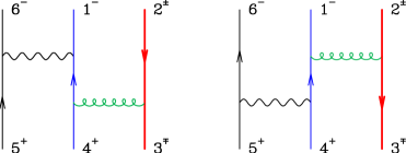
Figure 2: Feynman graphs that enter the calculation of the lowest order amplitude. The massive quarks are represented by the heavy (red) line, the wavy line denotes a W𝑊W boson and as usual the helical line denotes a gluon.

We shall consider the process,

0q(k1)+Q¯(p2)+Q(p3)+q¯(k4)+¯(k5)+(k6),0𝑞subscript𝑘1¯𝑄subscript𝑝2𝑄subscript𝑝3¯𝑞subscript𝑘4¯subscript𝑘5subscript𝑘60\to q(k_{1})+{\bar{Q}}(p_{2})+{\vphantom{{\bar{Q}}}{Q}}(p_{3})+{\bar{q}}(k_{4})+\bar{\ell}(k_{5})+\ell(k_{6})\;, (19)

both at tree level and including the one-loop QCD corrections. The process is mediated by the exchange of a W𝑊W-boson which decays into an antilepton-lepton pair with momenta labelled by k5subscript𝑘5k_{5} and k6subscript𝑘6k_{6}, as shown in Fig. 2. The V-A structure of the charged weak interaction ensures that the lepton and massless-quark lines will have fixed helicity. Thus the outgoing lepton (6) will be always left-handed and the outgoing antilepton (5) always right-handed. With this understanding we can often drop the lepton labels from the specification of the amplitude.

III.1 Colour decomposition

As noted above we shall suppress the labels for the outgoing leptons 555 and 666 which play no role in the colour decomposition. The colour decomposition for the tree graphs is,

𝒜6tree(1q,2Q¯,3Q,4q¯)=gW2g2𝒫W(s56)A6tree(1q,2Q¯,3Q,4q¯)(δj1j¯2δj3j¯41Ncδj1j¯4δj3j¯2).subscriptsuperscript𝒜tree6subscript1𝑞subscript2¯𝑄subscript3𝑄subscript4¯𝑞superscriptsubscript𝑔𝑊2superscript𝑔2subscript𝒫𝑊subscript𝑠56subscriptsuperscript𝐴tree6subscript1𝑞subscript2¯𝑄subscript3𝑄subscript4¯𝑞superscriptsubscript𝛿subscript𝑗1subscript¯𝑗2superscriptsubscript𝛿subscript𝑗3subscript¯𝑗41subscript𝑁𝑐superscriptsubscript𝛿subscript𝑗1subscript¯𝑗4superscriptsubscript𝛿subscript𝑗3subscript¯𝑗2{\cal A}^{\rm tree}_{6}(1_{\vphantom{{\bar{q}}}{q}},2_{\bar{Q}},3_{\vphantom{{\bar{Q}}}{Q}},4_{\bar{q}})=g_{W}^{2}g^{2}\;{\cal P}_{W}(s_{56})\;A^{\rm tree}_{6}(1_{\vphantom{{\bar{q}}}{q}},2_{\bar{Q}},3_{\vphantom{{\bar{Q}}}{Q}},4_{\bar{q}})\;\Bigl{(}\delta_{j_{1}}^{{\;\bar{j}}_{2}}\,\delta_{j_{3}}^{{\;\bar{j}}_{4}}\,-\frac{1}{N_{c}}\delta_{j_{1}}^{{\;\bar{j}}_{4}}\,\delta_{j_{3}}^{{\;\bar{j}}_{2}}\,\Bigr{)}\;. (20)

In Eq. (20) we have introduced the strong coupling constant, g𝑔g, and the weak coupling, gWsubscript𝑔𝑊g_{W}, defined through,

αS=g24π,GF2=gW28MW2.formulae-sequencesubscript𝛼𝑆superscript𝑔24𝜋subscript𝐺𝐹2superscriptsubscript𝑔𝑊28superscriptsubscript𝑀𝑊2\alpha_{S}=\frac{g^{2}}{4\pi}\;,\qquad\frac{G_{F}}{\sqrt{2}}=\frac{g_{W}^{2}}{8M_{W}^{2}}\;. (21)

The Breit-Wigner factor 𝒫W(s)subscript𝒫𝑊𝑠{\cal P}_{W}(s) is given by,

𝒫W(s)=ssMW2+iΓWMW.subscript𝒫𝑊𝑠𝑠𝑠superscriptsubscript𝑀𝑊2𝑖subscriptΓ𝑊subscript𝑀𝑊{\cal P}_{W}(s)=\frac{s}{s-M_{W}^{2}+i\,\Gamma_{W}\,M_{W}}\,. (22)

The indices j1,j3,(j¯2,j¯4)subscript𝑗1subscript𝑗3subscript¯𝑗2subscript¯𝑗4j_{1},j_{3},({\;\bar{j}}_{2},{\;\bar{j}}_{4}) denote the colour labels of the corresponding quark (antiquark) lines.

At one loop the colour decomposition is given by,

𝒜61loop(1q,2Q¯,3Q,4q¯)=gW2g4cΓ𝒫W(s56)superscriptsubscript𝒜61loopsubscript1𝑞subscript2¯𝑄subscript3𝑄subscript4¯𝑞superscriptsubscript𝑔𝑊2superscript𝑔4subscript𝑐Γsubscript𝒫𝑊subscript𝑠56\displaystyle{\cal A}_{6}^{1\rm-loop}(1_{\vphantom{{\bar{q}}}{q}},2_{\bar{Q}},3_{\vphantom{{\bar{Q}}}{Q}},4_{\bar{q}})=g_{W}^{2}g^{4}c_{\Gamma}\;{\cal P}_{W}(s_{56})\; (23)
×\displaystyle\times [Ncδj1j¯2δj3j¯4A6;1(1q,2Q¯,3Q,4q¯)+δj1j¯4δj3j¯2A6;2(1q,2Q¯,3Q,4q¯)],delimited-[]subscript𝑁𝑐superscriptsubscript𝛿subscript𝑗1subscript¯𝑗2superscriptsubscript𝛿subscript𝑗3subscript¯𝑗4subscript𝐴61subscript1𝑞subscript2¯𝑄subscript3𝑄subscript4¯𝑞superscriptsubscript𝛿subscript𝑗1subscript¯𝑗4superscriptsubscript𝛿subscript𝑗3subscript¯𝑗2subscript𝐴62subscript1𝑞subscript2¯𝑄subscript3𝑄subscript4¯𝑞\displaystyle\Bigl{[}N_{c}\,\delta_{j_{1}}^{{\;\bar{j}}_{2}}\,\delta_{j_{3}}^{{\;\bar{j}}_{4}}\,A_{6;1}(1_{\vphantom{{\bar{q}}}{q}},2_{\bar{Q}},3_{\vphantom{{\bar{Q}}}{Q}},4_{\bar{q}})+\delta_{j_{1}}^{{\;\bar{j}}_{4}}\,\delta_{j_{3}}^{{\;\bar{j}}_{2}}\,A_{6;2}(1_{\vphantom{{\bar{q}}}{q}},2_{\bar{Q}},3_{\vphantom{{\bar{Q}}}{Q}},4_{\bar{q}})\Bigr{]}\;,

where the overall factor cΓsubscript𝑐Γc_{\Gamma} is,

cΓ=1(4π)2ϵΓ(1+ϵ)Γ2(1ϵ)Γ(12ϵ).subscript𝑐Γ1superscript4𝜋2italic-ϵΓ1italic-ϵsuperscriptΓ21italic-ϵΓ12italic-ϵc_{\Gamma}=\frac{1}{(4\pi)^{2-\epsilon}}\frac{\Gamma(1+\epsilon)\Gamma^{2}(1-\epsilon)}{\Gamma(1-2\epsilon)}\ . (24)

The interference of the one-loop amplitude with the lowest order, summed over initial and final colours, is given by,

colours[𝒜6𝒜6]NLOsubscriptcolourssubscriptdelimited-[]superscriptsubscript𝒜6subscript𝒜6NLO\displaystyle\sum_{{\rm colours}}[{\cal A}_{6}^{*}{\cal A}_{6}]_{{\rm NLO}} =\displaystyle= 2gW4g6cΓ(Nc21)Nc|𝒫W(s56)|22superscriptsubscript𝑔𝑊4superscript𝑔6subscript𝑐Γsuperscriptsubscript𝑁𝑐21subscript𝑁𝑐superscriptsubscript𝒫𝑊subscript𝑠562\displaystyle 2g_{W}^{4}\,g^{6}c_{\Gamma}\,(N_{c}^{2}-1)N_{c}\;|{\cal P}_{W}(s_{56})|^{2} (25)
×\displaystyle\times Re{[A6tree(1q,2,3,4q¯)]A6;1(1q,2,3,4q¯)}.Resuperscriptdelimited-[]superscriptsubscript𝐴6treesubscript1𝑞23subscript4¯𝑞subscript𝐴61subscript1𝑞23subscript4¯𝑞\displaystyle{\rm Re}\Big{\{}[A_{6}^{\rm tree}(1_{q},2,3,4_{\bar{q}})]^{*}A_{6;1}(1_{q},2,3,4_{\bar{q}})\Big{\}}\;.

Therefore A6;2subscript𝐴62A_{6;2} plays no role in the calculation of NLO corrections.

III.2 Tree level amplitudes

The tree level amplitudes can be calculated using the diagrams of Fig. 2. The {+}\{-+\} amplitude, expressed in terms of the momenta kisubscript𝑘𝑖k_{i}, is identical to the massless result as a consequence of Eq. (12),

iA6tree(1q,2Q¯+,3Q,4q¯+,5¯+,6)𝑖subscriptsuperscript𝐴tree6superscriptsubscript1𝑞superscriptsubscript2¯𝑄superscriptsubscript3𝑄superscriptsubscript4¯𝑞superscriptsubscript5¯superscriptsubscript6\displaystyle-iA^{{\rm tree}}_{6}(1_{\vphantom{{\bar{q}}}{q}}^{-},2_{\bar{Q}}^{+},3_{\vphantom{{\bar{Q}}}{Q}}^{-},4_{\bar{q}}^{+},5_{\overline{\ell}}^{+},6_{\ell}^{-}) =\displaystyle= [1 3[4 5]6|(1+3)|2]s23s56s123[4 2]1 6[5|(2+4)|3s23s56s234]\displaystyle\left[\frac{\left\langle 1\,3\right\rangle\left[4\,5\right]\langle\mskip-1.0mu{6}|(1+3)|{2}\mskip-1.0mu]}{s_{23}s_{56}s_{123}}-\frac{\left[4\,2\right]\left\langle 1\,6\right\rangle[\mskip-1.0mu{5}|(2+4)|{3}\mskip-1.0mu\rangle}{s_{23}s_{56}s_{234}}\right] (26)
\displaystyle\equiv [{1 3[4 5]6|(1+3)|2]s23s56s123}{flip}],\displaystyle\left[\Bigg{\{}\frac{\left\langle 1\,3\right\rangle\left[4\,5\right]\langle\mskip-1.0mu{6}|(1+3)|{2}\mskip-1.0mu]}{s_{23}s_{56}s_{123}}\Bigg{\}}-\Bigg{\{}{\rm flip}\Bigg{\}}\right]\;,

where we have introduced the symmetry,

flip:(14),(23),(56),[].{\rm flip}:(1\leftrightarrow 4),\;(2\leftrightarrow 3),\;(5\leftrightarrow 6),\;[~{}]\leftrightarrow\langle~{}\rangle\;. (27)

The {}\{--\} amplitude is given by,

\displaystyle- iA6tree(1q,2Q¯,3Q,4q¯+,5¯+,6)=𝒩𝑖subscriptsuperscript𝐴tree6superscriptsubscript1𝑞superscriptsubscript2¯𝑄superscriptsubscript3𝑄superscriptsubscript4¯𝑞superscriptsubscript5¯superscriptsubscript6subscript𝒩absent\displaystyle iA^{{\rm tree}}_{6}(1_{\vphantom{{\bar{q}}}{q}}^{-},2_{\bar{Q}}^{-},3_{\vphantom{{\bar{Q}}}{Q}}^{-},4_{\bar{q}}^{+},5_{\overline{\ell}}^{+},6_{\ell}^{-})={\cal N}_{--} (28)
×[{[4 5](6|(1+2)|3]3 16|(1+3)|2]2 1s23s56s123)}+{flip}],\displaystyle\hskip 42.67912pt\times\left[\Bigg{\{}\left[4\,5\right]\left(\frac{\langle\mskip-1.0mu{6}|(1+2)|{3}\mskip-1.0mu]\left\langle 3\,1\right\rangle-\langle\mskip-1.0mu{6}|(1+3)|{2}\mskip-1.0mu]\left\langle 2\,1\right\rangle}{s_{23}s_{56}s_{123}}\right)\Bigg{\}}+\Bigg{\{}{\rm flip}\Bigg{\}}\right]\;,

with the mass-dependent normalization factor given in Eq. (14). The amplitudes for A6tree(1,2,3+,4+,6,5+)subscriptsuperscript𝐴tree6superscript1superscript2superscript3superscript4superscript6superscript5A^{{\rm tree}}_{6}(1^{-},2^{-},3^{+},4^{+},6^{-},5^{+}) and A6tree(1,2+,3+,4+,6,5+)subscriptsuperscript𝐴tree6superscript1superscript2superscript3superscript4superscript6superscript5A^{{\rm tree}}_{6}(1^{-},2^{+},3^{+},4^{+},6^{-},5^{+}) can be easily obtained by reference to Eqs. (12,II.1),

A6tree(1q,2Q¯,3Q+,4q¯+,5¯+,6)subscriptsuperscript𝐴tree6superscriptsubscript1𝑞superscriptsubscript2¯𝑄superscriptsubscript3𝑄superscriptsubscript4¯𝑞superscriptsubscript5¯superscriptsubscript6\displaystyle A^{{\rm tree}}_{6}(1_{\vphantom{{\bar{q}}}{q}}^{-},2_{\bar{Q}}^{-},3_{\vphantom{{\bar{Q}}}{Q}}^{+},4_{\bar{q}}^{+},5_{\overline{\ell}}^{+},6_{\ell}^{-}) =\displaystyle= A6tree(1q,3Q¯+,2Q,4q¯+,5¯+,6),subscriptsuperscript𝐴tree6superscriptsubscript1𝑞superscriptsubscript3¯𝑄superscriptsubscript2𝑄superscriptsubscript4¯𝑞superscriptsubscript5¯superscriptsubscript6\displaystyle A^{{\rm tree}}_{6}(1_{\vphantom{{\bar{q}}}{q}}^{-},3_{\bar{Q}}^{+},2_{\vphantom{{\bar{Q}}}{Q}}^{-},4_{\bar{q}}^{+},5_{\overline{\ell}}^{+},6_{\ell}^{-})\;, (29)
A6tree(1q,2Q¯+,3Q+,4q¯+,5¯+,6)subscriptsuperscript𝐴tree6superscriptsubscript1𝑞superscriptsubscript2¯𝑄superscriptsubscript3𝑄superscriptsubscript4¯𝑞superscriptsubscript5¯superscriptsubscript6\displaystyle A^{{\rm tree}}_{6}(1_{\vphantom{{\bar{q}}}{q}}^{-},2_{\bar{Q}}^{+},3_{\vphantom{{\bar{Q}}}{Q}}^{+},4_{\bar{q}}^{+},5_{\overline{\ell}}^{+},6_{\ell}^{-}) =\displaystyle= flip[A6tree(1q,2Q¯,3Q,4q¯+,5¯+,6)].flipdelimited-[]subscriptsuperscript𝐴tree6superscriptsubscript1𝑞superscriptsubscript2¯𝑄superscriptsubscript3𝑄superscriptsubscript4¯𝑞superscriptsubscript5¯superscriptsubscript6\displaystyle-{\rm flip}\left[A^{{\rm tree}}_{6}(1_{\vphantom{{\bar{q}}}{q}}^{-},2_{\bar{Q}}^{-},3_{\vphantom{{\bar{Q}}}{Q}}^{-},4_{\bar{q}}^{+},5_{\overline{\ell}}^{+},6_{\ell}^{-})\right]\;. (30)

III.3 Decomposition of one-loop amplitudes into primitive amplitudes

Following Ref. Bern:1997sc we can decompose the full one-loop amplitude into gauge invariant primitive amplitudes,

A6;1(1q,2Q¯,3Q,4q¯)subscript𝐴61subscript1𝑞subscript2¯𝑄subscript3𝑄subscript4¯𝑞\displaystyle A_{6;1}(1_{\vphantom{{\bar{q}}}{q}},2_{\bar{Q}},3_{\vphantom{{\bar{Q}}}{Q}},4_{\bar{q}}) =\displaystyle= A6lc(1,2,3,4)2N2(A6cb(1,2,3,4)+A6lc(1,2,3,4))subscriptsuperscript𝐴lc612342superscript𝑁2subscriptsuperscript𝐴cb61234subscriptsuperscript𝐴lc61234\displaystyle A^{\rm lc}_{6}(1,2,3,4)-\frac{2}{N^{2}}(A^{\rm cb}_{6}(1,2,3,4)+A^{\rm lc}_{6}(1,2,3,4))
\displaystyle- 1N2A6sl(1,2,3,4)nlfNA6lf(1,2,3,4)nhfNA6hf(1,2,3,4),1superscript𝑁2subscriptsuperscript𝐴sl61234subscript𝑛lf𝑁subscriptsuperscript𝐴lf61234subscript𝑛hf𝑁subscriptsuperscript𝐴hf61234\displaystyle\frac{1}{N^{2}}A^{\rm sl}_{6}(1,2,3,4)-\frac{n_{{\rm lf}}}{N}A^{\rm lf}_{6}(1,2,3,4)-\frac{n_{{\rm hf}}}{N}A^{\rm hf}_{6}(1,2,3,4)\;,
A6;2(1q,2Q¯,3Q,4q¯)subscript𝐴62subscript1𝑞subscript2¯𝑄subscript3𝑄subscript4¯𝑞\displaystyle A_{6;2}(1_{\vphantom{{\bar{q}}}{q}},2_{\bar{Q}},3_{\vphantom{{\bar{Q}}}{Q}},4_{\bar{q}}) =\displaystyle= A6cb(1,2,3,4)+1N2(A6lc(1,2,3,4)+A6cb(1,2,3,4))subscriptsuperscript𝐴cb612341superscript𝑁2subscriptsuperscript𝐴lc61234subscriptsuperscript𝐴cb61234\displaystyle A^{\rm cb}_{6}(1,2,3,4)+\frac{1}{N^{2}}(A^{\rm lc}_{6}(1,2,3,4)+A^{\rm cb}_{6}(1,2,3,4)) (31)
+\displaystyle+ 1N2A6sl(1,2,3,4)+nlfNA6lf(1,2,3,4)+nhfNA6hf(1,2,3,4).1superscript𝑁2subscriptsuperscript𝐴sl61234subscript𝑛lf𝑁subscriptsuperscript𝐴lf61234subscript𝑛hf𝑁subscriptsuperscript𝐴hf61234\displaystyle\frac{1}{N^{2}}A^{\rm sl}_{6}(1,2,3,4)+\frac{n_{{\rm lf}}}{N}A^{\rm lf}_{6}(1,2,3,4)+\frac{n_{{\rm hf}}}{N}A^{\rm hf}_{6}(1,2,3,4)\;.

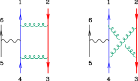
A6lcsubscriptsuperscript𝐴lc6A^{\rm lc}_{6} is the primitive amplitude containing the leading colour box and A6cbsubscriptsuperscript𝐴cb6A^{\rm cb}_{6} is the primitive amplitude containing the crossed box. The parent diagrams are shown in Fig. 3.
Refer to caption
Figure 3: Parent diagrams for the leading colour primitive A6lc(1,2,3,4)subscriptsuperscript𝐴lc61234A^{\rm lc}_{6}(1,2,3,4) and crossed box primitive A6cb(1,2,3,4)subscriptsuperscript𝐴cb61234A^{\rm cb}_{6}(1,2,3,4).

These two primitive amplitudes are related by,

A6cb(1qh1,2Q¯h2,3Qh3,4q¯h4)=A6lc(1qh1,3Q¯h3,2Qh2,4q¯h4).subscriptsuperscript𝐴cb6superscriptsubscript1𝑞subscript1superscriptsubscript2¯𝑄subscript2superscriptsubscript3𝑄subscript3superscriptsubscript4¯𝑞subscript4subscriptsuperscript𝐴lc6superscriptsubscript1𝑞subscript1superscriptsubscript3¯𝑄subscript3superscriptsubscript2𝑄subscript2superscriptsubscript4¯𝑞subscript4A^{\rm cb}_{6}(1_{\vphantom{{\bar{q}}}{q}}^{h_{1}},2_{\bar{Q}}^{h_{2}},3_{\vphantom{{\bar{Q}}}{Q}}^{h_{3}},4_{\bar{q}}^{h_{4}})=-A^{\rm lc}_{6}(1_{\vphantom{{\bar{q}}}{q}}^{h_{1}},3_{\bar{Q}}^{h_{3}},2_{\vphantom{{\bar{Q}}}{Q}}^{h_{2}},4_{\bar{q}}^{h_{4}})\;. (32)

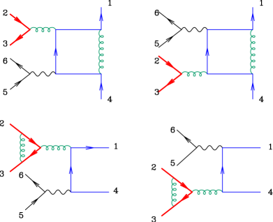
A6slsubscriptsuperscript𝐴sl6A^{\rm sl}_{6} is the primitive amplitude containing the subleading colour boxes, see Fig. 4,
Refer to caption
Figure 4: Parent diagrams for the subleading colour primitive amplitude, A6sl(1,2,3,4)subscriptsuperscript𝐴sl61234A^{\rm sl}_{6}(1,2,3,4).

and the primitive amplitude for the fermion-loop diagrams (light and heavy), A6lf,A6hfsubscriptsuperscript𝐴lf6subscriptsuperscript𝐴hf6A^{\rm lf}_{6},A^{\rm hf}_{6} is shown in Fig. 5.

Refer to caption
Figure 5: Diagrams for the fermion loop primitives A6lf(1,2,3,4)subscriptsuperscript𝐴lf61234A^{\rm lf}_{6}(1,2,3,4) and A6hf(1,2,3,4)subscriptsuperscript𝐴hf61234A^{\rm hf}_{6}(1,2,3,4).

We note that, just as at tree level, parity ensures that we need only compute a reduced set of amplitudes. For A6lcsubscriptsuperscript𝐴lc6A^{\rm lc}_{6} at one loop it is sufficient to calculate three of the four possible spin label combinations since (c.f. Eq. 30),

A6lc(1q,2Q¯+,3Q+,4q¯+,5¯+,6)=flip[A6lc(1q,2Q¯,3Q,4q¯+,5¯+,6)].subscriptsuperscript𝐴lc6superscriptsubscript1𝑞superscriptsubscript2¯𝑄superscriptsubscript3𝑄superscriptsubscript4¯𝑞superscriptsubscript5¯superscriptsubscript6flipdelimited-[]subscriptsuperscript𝐴lc6superscriptsubscript1𝑞superscriptsubscript2¯𝑄superscriptsubscript3𝑄superscriptsubscript4¯𝑞superscriptsubscript5¯superscriptsubscript6A^{\rm lc}_{6}(1_{\vphantom{{\bar{q}}}{q}}^{-},2_{\bar{Q}}^{+},3_{\vphantom{{\bar{Q}}}{Q}}^{+},4_{\bar{q}}^{+},5_{\overline{\ell}}^{+},6_{\ell}^{-})=-{\rm flip}\left[A^{\rm lc}_{6}(1_{\vphantom{{\bar{q}}}{q}}^{-},2_{\bar{Q}}^{-},3_{\vphantom{{\bar{Q}}}{Q}}^{-},4_{\bar{q}}^{+},5_{\overline{\ell}}^{+},6_{\ell}^{-})\right]\;. (33)

III.4 Structure of the calculation

In the presence of propagators with vanishing masses on internal lines the one-loop amplitude contains infrared and collinear divergences. In addition, the amplitude contains ultraviolet divergences. We regulate all of these divergences using dimensional regularization, continuing the loop integration to D=42ϵ𝐷42italic-ϵD=4-2\epsilon dimensions. The divergences then appear as poles in ϵitalic-ϵ\epsilon. For the primitive amplitudes the divergence structure is quite simple and we can separate the amplitude as follows,

A6j=[A6treeVj+iFj],superscriptsubscript𝐴6𝑗delimited-[]subscriptsuperscript𝐴tree6superscript𝑉𝑗𝑖superscript𝐹𝑗A_{6}^{j}=\Bigl{[}A^{\rm tree}_{6}V^{j}+i\,F^{j}\Bigr{]}\ , (34)

where Vjsuperscript𝑉𝑗V^{j} contains all the divergent pieces. In this equation A6jsuperscriptsubscript𝐴6𝑗A_{6}^{j} is any of the primitive amplitudes and the index j𝑗j runs over {lc,cb,sl,lf,hf}lccbsllfhf\{{\rm lc},{\rm cb},{\rm sl},{\rm lf},{\rm hf}\}. As we shall see later the simplicity of the pole structure gives useful constraints on the different terms contributing to the amplitude.

Refer to caption
Figure 6: Schematic diagram illustrating the decomposition in scalar integrals.

The calculation proceeds by noting that the primitive amplitudes can be expressed as a sum of scalar box, triangle, bubble and tadpole integrals and a rational part,

iA6j(1,2h2,3h3,4+,5+,6)=i1i2i3di1|i2|i3(h3,h2)D0(pi1,pi2,pi3)𝑖superscriptsubscript𝐴6𝑗superscript1superscript2subscript2superscript3subscript3superscript4superscript5superscript6subscriptsubscript𝑖1subscript𝑖2subscript𝑖3subscript𝑑subscript𝑖1subscript𝑖2subscript𝑖3subscript3subscript2subscript𝐷0subscript𝑝subscript𝑖1subscript𝑝subscript𝑖2subscript𝑝subscript𝑖3\displaystyle-iA_{6}^{j}(1^{-},2^{h_{2}},3^{h_{3}},4^{+},5^{+},6^{-})=\sum_{i_{1}i_{2}i_{3}}d_{i_{1}|i_{2}|i_{3}}(h_{3},h_{2})\;D_{0}(p_{i_{1}},p_{i_{2}},p_{i_{3}}) (35)
+\displaystyle+ i1i2ci1|i2(h3,h2)C0(pi1,pi2)+i1bi1(h3,h2)B0(pi1)+a(h3,h2)A0subscriptsubscript𝑖1subscript𝑖2subscript𝑐conditionalsubscript𝑖1subscript𝑖2subscript3subscript2subscript𝐶0subscript𝑝subscript𝑖1subscript𝑝subscript𝑖2subscriptsubscript𝑖1subscript𝑏subscript𝑖1subscript3subscript2subscript𝐵0subscript𝑝subscript𝑖1𝑎subscript3subscript2subscript𝐴0\displaystyle\sum_{i_{1}i_{2}}c_{i_{1}|i_{2}}(h_{3},h_{2})\;C_{0}(p_{i_{1}},p_{i_{2}})+\sum_{i_{1}}b_{i_{1}}(h_{3},h_{2})\;B_{0}(p_{i_{1}})+a(h_{3},h_{2})\;A_{0}
+\displaystyle+ Rj(1,2h2,3h3,4+,5+,6),superscript𝑅𝑗superscript1superscript2subscript2superscript3subscript3superscript4superscript5superscript6\displaystyle R^{j}(1^{-},2^{h_{2}},3^{h_{3}},4^{+},5^{+},6^{-})\;,

where the label j𝑗j runs over the values {lc,cb,sl,lf,hf}lccbsllfhf\{{\rm lc},{\rm cb},{\rm sl},{\rm lf},{\rm hf}\}. In this equation, illustrated in Fig. 6, the indices i1,i2,i3subscript𝑖1subscript𝑖2subscript𝑖3i_{1},i_{2},i_{3} run over all partitions of the cyclically ordered momenta. The coefficients d,c,b,a𝑑𝑐𝑏𝑎d,c,b,a of the scalar integrals in Eq. (35) also depend on the primitive amplitude index j𝑗j. In the following we shall suppress this dependence, but the primitive amplitude to which we are referring will be clear from the context. The functions A0subscript𝐴0A_{0}B0subscript𝐵0B_{0}C0subscript𝐶0C_{0}D0subscript𝐷0D_{0} are the scalar integrals defined in Appendix C. The mass labels have been suppressed in the scalar integrals in Eq. (35) because they are determined automatically by the propagators connecting the two external massive quarks. Values for these scalar integrals are obtained using the QCDLoop program Ellis:2007qk . By using four-dimensional unitarity methods Britto:2004nc ; Cachazo:2004kj ; Britto:2005ha ; Britto:2006sj ; Forde:2007mi , we obtain the coefficients, a𝑎ab𝑏bc𝑐cd𝑑d in the four-dimensional helicity (FDH) scheme Bern:2002zk . The rational terms require information from beyond four dimensions.

IV The results for primitive amplitude A6lcsubscriptsuperscript𝐴lc6A^{\rm lc}_{6}

IV.1 Divergent parts

For the leading colour primitive amplitude the divergent term which enters in Eq. (34) is given by Catani:2000ef ,

Vlc=1ϵ2[(μ22k4.p3)ϵ+(μ22k1.p2)ϵ(μ2m2)ϵ]+831ϵ.superscript𝑉𝑙𝑐1superscriptitalic-ϵ2delimited-[]superscriptsuperscript𝜇2formulae-sequence2subscript𝑘4subscript𝑝3italic-ϵsuperscriptsuperscript𝜇2formulae-sequence2subscript𝑘1subscript𝑝2italic-ϵsuperscriptsuperscript𝜇2superscript𝑚2italic-ϵ831italic-ϵV^{lc}=-\frac{1}{\epsilon^{2}}\Bigg{[}\Big{(}\frac{\mu^{2}}{-2k_{4}.p_{3}}\Big{)}^{\epsilon}+\Big{(}\frac{\mu^{2}}{-2k_{1}.p_{2}}\Big{)}^{\epsilon}-\Big{(}\frac{\mu^{2}}{m^{2}}\Big{)}^{\epsilon}\Bigg{]}+\frac{8}{3}\frac{1}{\epsilon}\;. (36)

IV.2 Calculation of the box coefficients

The five scalar box integrals that enter the leading colour amplitude are enumerated in Table 1.

      Scalar integral Coefficient       Scalar integral Coefficient
1. D0(k1,p2,p3;0,0,m,0)subscript𝐷0subscript𝑘1subscript𝑝2subscript𝑝300𝑚0D_{0}(k_{1},p_{2},p_{3};0,0,m,0) d1|2|3subscript𝑑123d_{1|2|3} 4. D0(p2,p3,k4;0,m,0,0)subscript𝐷0subscript𝑝2subscript𝑝3subscript𝑘40𝑚00D_{0}(p_{2},p_{3},k_{4};0,m,0,0) d2|3|4subscript𝑑234d_{2|3|4}
2. D0(k1,p2,p34;0,0,m,0)subscript𝐷0subscript𝑘1subscript𝑝2subscript𝑝3400𝑚0D_{0}(k_{1},p_{2},p_{34};0,0,m,0) d1|2|34subscript𝑑1234d_{1|2|34} 5. D0(p12,p3,k4;0,m,0,0)subscript𝐷0subscript𝑝12subscript𝑝3subscript𝑘40𝑚00D_{0}(p_{12},p_{3},k_{4};0,m,0,0) d12|3|4subscript𝑑1234d_{12|3|4}
3. D0(k1,p23,k4;0,0,0,0)subscript𝐷0subscript𝑘1subscript𝑝23subscript𝑘40000D_{0}(k_{1},p_{23},k_{4};0,0,0,0) d1|23|4subscript𝑑1234d_{1|23|4}
Table 1: Scalar box integrals appearing in the leading colour amplitude A6lc1,2,3,4)A_{6}^{lc}1,2,3,4) and the notation used in the text to denote their coefficients.

Of these, we directly calculate the coefficients of boxes 1–3 and obtain the remaining two by symmetry:

d2|3|4(h3,h2)subscript𝑑234subscript3subscript2\displaystyle d_{2|3|4}(h_{3},h_{2}) =\displaystyle= flip[d1|2|3(h2,h3)],flipdelimited-[]subscript𝑑123subscript2subscript3\displaystyle-\mbox{flip}\left[d_{1|2|3}(-h_{2},-h_{3})\right]\;,
d12|3|4(h3,h2)subscript𝑑1234subscript3subscript2\displaystyle d_{12|3|4}(h_{3},h_{2}) =\displaystyle= flip[d1|2|34(h2,h3)],flipdelimited-[]subscript𝑑1234subscript2subscript3\displaystyle-\mbox{flip}\left[d_{1|2|34}(-h_{2},-h_{3})\right]\;, (37)

where h3subscript3h_{3} and h2subscript2h_{2} represent the spin labels of the quark and antiquark respectively and the operation flip is defined in Eq. (27). When using the Rodrigo choice to decompose p2subscript𝑝2p_{2} and p3subscript𝑝3p_{3}, box 3 only gives a non-zero contribution for the spin-labels {,}\{-,-\} and {+,+}\{+,+\}.

The coefficients are computed using quadruple cuts with complex momenta Britto:2004nc . For boxes 1 and 2 the presence of a massive propagator leads to a more complicated parametrization of the loop momentum than in the purely massless case. The particular parameterizations that we have used are spelled out below.

IV.2.1 Calculation of d1|2|3subscript𝑑123d_{1|2|3}

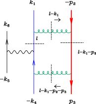
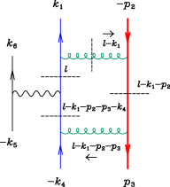
The cuts used to isolate this coefficient are depicted in Fig. 7, where we remind the reader that we work in the case that k12=k42=0superscriptsubscript𝑘12superscriptsubscript𝑘420k_{1}^{2}=k_{4}^{2}=0 and p22=p33=m2superscriptsubscript𝑝22superscriptsubscript𝑝33superscript𝑚2p_{2}^{2}=p_{3}^{3}=m^{2}. The loop momentum is subject to the following constraints,

l2=0,(lk1)2=0,(lk1p2)2=m2,(lk1p2p3)2=0,formulae-sequencesuperscript𝑙20formulae-sequencesuperscript𝑙subscript𝑘120formulae-sequencesuperscript𝑙subscript𝑘1subscript𝑝22superscript𝑚2superscript𝑙subscript𝑘1subscript𝑝2subscript𝑝320l^{2}=0,\;\;(l-k_{1})^{2}=0,\;\;(l-k_{1}-p_{2})^{2}=m^{2},\;\;(l-k_{1}-p_{2}-p_{3})^{2}=0,\;\; (38)
Refer to caption
Figure 7: Diagram for the calculation of the coefficient of the scalar integral D0(k1,p2,p3;0,0,m,0)subscript𝐷0subscript𝑘1subscript𝑝2subscript𝑝300𝑚0D_{0}(k_{1},p_{2},p_{3};0,0,m,0). The massive quark is represented by the heavy (red) line and unitarity cuts are represented by a dashed line.

Denoting l1=lk1subscript𝑙1𝑙subscript𝑘1l_{1}=l-k_{1} we have l1k1=0subscript𝑙1subscript𝑘10l_{1}\cdot k_{1}=0 so we must have either |l1|1similar-toketsubscript𝑙1ket1|l_{1}\rangle\sim|1\rangle or |l1]|1]|l_{1}]\sim|1], depending on the helicity of the internal gluons, in such a way that the 3-point qq¯g𝑞¯𝑞𝑔q\bar{q}g vertex is non-vanishing.

In the case [l1|[1|[l_{1}|\sim[1| we can write

l1μ=lμk1μsuperscriptsubscript𝑙1𝜇superscript𝑙𝜇superscriptsubscript𝑘1𝜇\displaystyle l_{1}^{\mu}=l^{\mu}-k_{1}^{\mu} =\displaystyle= s232[1|γμ𝟐|1][1|(𝟐+𝟑)𝟐|1]s232[1|γμ𝟐|1][1|𝟑𝟐|1],subscript𝑠232delimited-[]1superscript𝛾𝜇21delimited-[]12321subscript𝑠232delimited-[]1superscript𝛾𝜇21delimited-[]1321\displaystyle\frac{s_{23}}{2}\;\frac{[1|\gamma^{\mu}\hbox to0.0pt{$\;\!\!\not$\hss}{{\bf 2}}|1]}{[1|(\hbox to0.0pt{$\;\!\!\not$\hss}{{\bf 2}}+\hbox to0.0pt{$\;\!\!\not$\hss}{{\bf 3}})\hbox to0.0pt{$\;\!\!\not$\hss}{{\bf 2}}|1]}\equiv\frac{s_{23}}{2}\;\frac{[1|\gamma^{\mu}\hbox to0.0pt{$\;\!\!\not$\hss}{{\bf 2}}|1]}{[1|\hbox to0.0pt{$\;\!\!\not$\hss}{{\bf 3}}\hbox to0.0pt{$\;\!\!\not$\hss}{{\bf 2}}|1]}\;,
l123μ=l1μp2μp3μsubscriptsuperscript𝑙𝜇123superscriptsubscript𝑙1𝜇superscriptsubscript𝑝2𝜇superscriptsubscript𝑝3𝜇\displaystyle l^{\mu}_{123}=l_{1}^{\mu}-p_{2}^{\mu}-p_{3}^{\mu} =\displaystyle= 12[1|(𝟐+𝟑)γμ(𝟐+𝟑)𝟐|1][1|𝟑𝟐|1],12delimited-[]123superscript𝛾𝜇2321delimited-[]1321\displaystyle-\frac{1}{2}\;\frac{[1|(\hbox to0.0pt{$\;\!\!\not$\hss}{{\bf 2}}+\hbox to0.0pt{$\;\!\!\not$\hss}{{\bf 3}})\gamma^{\mu}(\hbox to0.0pt{$\;\!\!\not$\hss}{{\bf 2}}+\hbox to0.0pt{$\;\!\!\not$\hss}{{\bf 3}})\hbox to0.0pt{$\;\!\!\not$\hss}{{\bf 2}}|1]}{[1|\hbox to0.0pt{$\;\!\!\not$\hss}{{\bf 3}}\hbox to0.0pt{$\;\!\!\not$\hss}{{\bf 2}}|1]}\;, (39)

where the boldface momenta denote massive vectors. By inspection, it is clear that this parametrization of the loop momentum lμsuperscript𝑙𝜇l^{\mu} satisfies the constraints in Eq. (38). Correspondingly in the case l1|1|similar-tobrasubscript𝑙1bra1\langle l_{1}|\sim\langle 1| we can write

l1μ=lμk1μsuperscriptsubscript𝑙1𝜇superscript𝑙𝜇superscriptsubscript𝑘1𝜇\displaystyle l_{1}^{\mu}=l^{\mu}-k_{1}^{\mu} =\displaystyle= s2321|𝟐γμ|11|𝟐(𝟐+𝟑)|1s2321|𝟐γμ|11|𝟐𝟑|1,subscript𝑠232quantum-operator-product12superscript𝛾𝜇1quantum-operator-product12231subscript𝑠232quantum-operator-product12superscript𝛾𝜇1quantum-operator-product1231\displaystyle\frac{s_{23}}{2}\;\frac{\langle 1|\hbox to0.0pt{$\;\!\!\not$\hss}{{\bf 2}}\gamma^{\mu}|1\rangle}{\langle 1|\hbox to0.0pt{$\;\!\!\not$\hss}{{\bf 2}}(\hbox to0.0pt{$\;\!\!\not$\hss}{{\bf 2}}+\hbox to0.0pt{$\;\!\!\not$\hss}{{\bf 3}})|1\rangle}\equiv\frac{s_{23}}{2}\;\frac{\langle 1|\hbox to0.0pt{$\;\!\!\not$\hss}{{\bf 2}}\gamma^{\mu}|1\rangle}{\langle 1|\hbox to0.0pt{$\;\!\!\not$\hss}{{\bf 2}}\hbox to0.0pt{$\;\!\!\not$\hss}{{\bf 3}}|1\rangle}\;,
l123μ=l1μp2μp3μsubscriptsuperscript𝑙𝜇123superscriptsubscript𝑙1𝜇superscriptsubscript𝑝2𝜇superscriptsubscript𝑝3𝜇\displaystyle l^{\mu}_{123}=l_{1}^{\mu}-p_{2}^{\mu}-p_{3}^{\mu} =\displaystyle= 121|𝟐(𝟐+𝟑)γμ(𝟐+𝟑)|11|𝟐𝟑|1.12quantum-operator-product1223superscript𝛾𝜇231quantum-operator-product1231\displaystyle-\frac{1}{2}\;\frac{\langle 1|\hbox to0.0pt{$\;\!\!\not$\hss}{{\bf 2}}(\hbox to0.0pt{$\;\!\!\not$\hss}{{\bf 2}}+\hbox to0.0pt{$\;\!\!\not$\hss}{{\bf 3}})\gamma^{\mu}(\hbox to0.0pt{$\;\!\!\not$\hss}{{\bf 2}}+\hbox to0.0pt{$\;\!\!\not$\hss}{{\bf 3}})|1\rangle}{\langle 1|\hbox to0.0pt{$\;\!\!\not$\hss}{{\bf 2}}\hbox to0.0pt{$\;\!\!\not$\hss}{{\bf 3}}|1\rangle}\;. (40)

Note that the denominator in Eq. (40) simplifies when expressed in terms of massless momenta,

1|𝟐𝟑|1=β1 2[2 3]3 1,quantum-operator-product1231𝛽delimited-⟨⟩12delimited-[]23delimited-⟨⟩31{\langle 1|\hbox to0.0pt{$\;\!\!\not$\hss}{{\bf 2}}\hbox to0.0pt{$\;\!\!\not$\hss}{{\bf 3}}|1\rangle}=\beta\left\langle 1\,2\right\rangle\left[2\,3\right]\left\langle 3\,1\right\rangle\;, (41)

As an example, we will calculate the coefficient of this box integral for the spin label choice {,+}\{-,+\}. The box coefficient is given by the formula,

d1|2|3(,+)subscript𝑑123\displaystyle d_{1|2|3}(-,+) \displaystyle\equiv 12ha,hbd1|2|3[ha,hb](,+)12subscriptsubscript𝑎subscript𝑏superscriptsubscript𝑑123subscript𝑎subscript𝑏\displaystyle\frac{1}{2}\sum_{h_{a},h_{b}}d_{1|2|3}^{\,[h_{a},h_{b}]}(-,+) (42)
=\displaystyle= 12ha,hbA3(1q,lq¯+,l1ha)×A5(lq,4q¯+,l123hb,5l¯+,6l)12subscriptsubscript𝑎subscript𝑏subscript𝐴3superscriptsubscript1𝑞superscriptsubscript𝑙¯𝑞superscriptsubscript𝑙1subscript𝑎subscript𝐴5superscriptsubscript𝑙𝑞superscriptsubscript4¯𝑞superscriptsubscript𝑙123subscript𝑏superscriptsubscript5¯𝑙superscriptsubscript6𝑙\displaystyle\frac{1}{2}\sum_{h_{a},h_{b}}A_{3}(1_{\vphantom{{\bar{q}}}{q}}^{-},-{l_{\bar{q}}^{+}},l_{1}^{h_{a}})\times A_{5}({l_{\vphantom{{\bar{q}}}{q}}^{-}},4_{\bar{q}}^{+},-l_{123}^{h_{b}},5_{\bar{l}}^{+},6_{\vphantom{{\bar{l}}}{l}}^{-})
×A4(l1ha,2Q¯+,3Q,l123hb)×(i)[(lk1p2)2m2],absentsubscript𝐴4superscriptsubscript𝑙1subscript𝑎superscriptsubscript2¯𝑄superscriptsubscript3𝑄superscriptsubscript𝑙123subscript𝑏𝑖delimited-[]superscript𝑙subscript𝑘1subscript𝑝22superscript𝑚2\displaystyle\qquad\times A_{4}(-l_{1}^{-h_{a}},2_{\bar{Q}}^{+},3_{\vphantom{{\bar{Q}}}{Q}}^{-},l_{123}^{-h_{b}})\times(-i)\left[(l-k_{1}-p_{2})^{2}-m^{2}\right]\;,

with the loop momenta fixed according to the constraints above, i.e. lμsuperscript𝑙𝜇l^{\mu} is given by either Eq. (39) or (40) above. In this formula we have for brevity suppressed the gluon particle labels. Note that we have not explicitly cut the heavy quark propagator but, equivalently, have simply written the full gQ¯Qg𝑔¯𝑄𝑄𝑔g{\bar{Q}}{\vphantom{{\bar{Q}}}{Q}}g amplitude and multiplied by the cut propagator. Since the gQ¯Qg𝑔¯𝑄𝑄𝑔g{\bar{Q}}{\vphantom{{\bar{Q}}}{Q}}g amplitudes with the same helicity gluons vanish (c.f. Eq. (B.1)), the coefficient receives only two contributions.

Let us first inspect the assignment ha=hb=+1subscript𝑎subscript𝑏1h_{a}=-h_{b}=+1. We note that it is simplest to manipulate the gQ¯Qg𝑔¯𝑄𝑄𝑔g{\bar{Q}}{\vphantom{{\bar{Q}}}{Q}}g amplitude, (Eq. (B.1) first line), using the Schouten identity, Eq. (118), into an alternative form in order to take full advantage of the vanishing of the cut propagator,

iA4(l1,2Q¯+,3Q,l123+)[(l1p2)2m2]𝑖subscript𝐴4superscriptsubscript𝑙1superscriptsubscript2¯𝑄superscriptsubscript3𝑄superscriptsubscript𝑙123delimited-[]superscriptsubscript𝑙1subscript𝑝22superscript𝑚2\displaystyle-iA_{4}(-l_{1}^{-},2_{\bar{Q}}^{+},3_{\vphantom{{\bar{Q}}}{Q}}^{-},l_{123}^{+})\left[(l_{1}-p_{2})^{2}-m^{2}\right] =\displaystyle= [2l123]2l1|𝟐|l123][l1l123][2 3]\displaystyle\frac{\left[2\,l_{123}\right]^{2}\langle\mskip-1.0mu{l_{1}}|\hbox to0.0pt{$\;\!\!\not$\hss}{\bf 2}|{l_{123}}\mskip-1.0mu]}{\left[l_{1}\,l_{123}\right]\left[2\,3\right]} (43)
=\displaystyle= [2l123]2([l1l123]l1|𝟐|3]l1|𝟐|l1][3l123])[l1 3][l1l123][2 3]\displaystyle-\frac{\left[2\,l_{123}\right]^{2}\left(\left[l_{1}\,l_{123}\right]\langle\mskip-1.0mu{l_{1}}|\hbox to0.0pt{$\;\!\!\not$\hss}{\bf 2}|{3}\mskip-1.0mu]-\langle\mskip-1.0mu{l_{1}}|\hbox to0.0pt{$\;\!\!\not$\hss}{\bf 2}|{l_{1}}\mskip-1.0mu]\left[3\,l_{123}\right]\right)}{\left[l_{1}\,3\right]\left[l_{1}\,l_{123}\right]\left[2\,3\right]}
=\displaystyle= [2l123]2[l1 3][2 3](l1|𝟐|3][3l123]l1|𝟐|l1][l1l123]).\displaystyle-\frac{\left[2\,l_{123}\right]^{2}}{\left[l_{1}\,3\right]\left[2\,3\right]}\left(\langle\mskip-1.0mu{l_{1}}|\hbox to0.0pt{$\;\!\!\not$\hss}{\bf 2}|{3}\mskip-1.0mu]-\frac{\left[3\,l_{123}\right]\langle\mskip-1.0mu{l_{1}}|\hbox to0.0pt{$\;\!\!\not$\hss}{\bf 2}|{l_{1}}\mskip-1.0mu]}{\left[l_{1}\,l_{123}\right]}\right)\;.

On shell, (l1p2)2m2l1|𝟐|l1]=0(l_{1}-p_{2})^{2}-m^{2}\equiv\langle\mskip-1.0mu{l_{1}}|\hbox to0.0pt{$\;\!\!\not$\hss}{\bf 2}|{l_{1}}\mskip-1.0mu]=0 and we can simply discard the second term in this equation. Using results for the other amplitudes presented in Appendix B we find that,

d1|2|3[+,](,+)=[ll1]2[l 1]×[4 5]2[4l123][ll123][6 5]×β+[2l123]22l1[l1 3],superscriptsubscript𝑑123superscriptdelimited-[]𝑙subscript𝑙12delimited-[]𝑙1superscriptdelimited-[]452delimited-[]4subscript𝑙123delimited-[]𝑙subscript𝑙123delimited-[]65subscript𝛽superscriptdelimited-[]2subscript𝑙1232delimited-⟨⟩2subscript𝑙1delimited-[]subscript𝑙13d_{1|2|3}^{\,[+,-]}(-,+)=\frac{\left[l\,l_{1}\right]^{2}}{\left[l\,1\right]}\times\frac{\left[4\,5\right]^{2}}{\left[4\,l_{123}\right]\left[l\,l_{123}\right]\left[6\,5\right]}\times\frac{\beta_{+}\left[2\,l_{123}\right]^{2}\left\langle 2\,l_{1}\right\rangle}{\left[l_{1}\,3\right]}\;, (44)

where we have simplified the gQ¯Qg𝑔¯𝑄𝑄𝑔g{\bar{Q}}{\vphantom{{\bar{Q}}}{Q}}g amplitude further using the decomposition of p2subscript𝑝2p_{2} in terms of k2subscript𝑘2k_{2} and k3subscript𝑘3k_{3}. Since the propagator l𝑙l does not have a simple decomposition in terms of external momenta, it is simplest to eliminate it by multiplying this expression in numerator and denominator by a factor 4ll123ldelimited-⟨⟩4𝑙delimited-⟨⟩subscript𝑙123𝑙\left\langle 4\,l\right\rangle\left\langle l_{123}\,l\right\rangle. After some simplification this yields,

d1|2|3[+,](,+)=β+[4 5]24 1s123[6 5]l123 1[1l1][2l123]22l14l1[4l123][l1 3],superscriptsubscript𝑑123subscript𝛽superscriptdelimited-[]452delimited-⟨⟩41subscript𝑠123delimited-[]65delimited-⟨⟩subscript𝑙1231delimited-[]1subscript𝑙1superscriptdelimited-[]2subscript𝑙1232delimited-⟨⟩2subscript𝑙1delimited-⟨⟩4subscript𝑙1delimited-[]4subscript𝑙123delimited-[]subscript𝑙13d_{1|2|3}^{\,[+,-]}(-,+)=\frac{\beta_{+}\left[4\,5\right]^{2}\left\langle 4\,1\right\rangle}{s_{123}\left[6\,5\right]}\,\frac{\left\langle l_{123}\,1\right\rangle\left[1\,l_{1}\right]\left[2\,l_{123}\right]^{2}\left\langle 2\,l_{1}\right\rangle}{\left\langle 4\,l_{1}\right\rangle\left[4\,l_{123}\right]\left[l_{1}\,3\right]}\;, (45)

This is now in a form where we can use the loop momenta definitions given in Eq. (40) with spinors identified by, for example, using the identity, lμ=12l|γμ|l]l^{\mu}=\frac{1}{2}\langle\mskip-1.0mu{l}|\gamma^{\mu}|{l}\mskip-1.0mu]. We can thus make the replacements:

l123 11|𝟐(𝟐+𝟑)|11|𝟐𝟑|1=1,[1l1]s231|𝟐|1]1|𝟐𝟑|1,[4l123][4|(𝟐+𝟑)|1=1|2+3|4],[2l123][2|(𝟐+𝟑)|1=[2 3]3 1,2l12 1,4l14 1,[l1 3]s231|𝟐|3]1|𝟐𝟑|1=s23β+1 2[2 3]1|𝟐𝟑|1.\begin{array}[]{lll}\left\langle l_{123}\,1\right\rangle&\longrightarrow-\frac{\displaystyle\langle 1|\hbox to0.0pt{$\;\!\!\not$\hss}{{\bf 2}}(\hbox to0.0pt{$\;\!\!\not$\hss}{{\bf 2}}+\hbox to0.0pt{$\;\!\!\not$\hss}{{\bf 3}})|1\rangle}{\displaystyle\langle 1|\hbox to0.0pt{$\;\!\!\not$\hss}{{\bf 2}}\hbox to0.0pt{$\;\!\!\not$\hss}{{\bf 3}}|1\rangle}=-1\;,&\left[1\,l_{1}\right]\longrightarrow-s_{23}\frac{\displaystyle\langle\mskip-1.0mu{1}|\hbox to0.0pt{$\;\!\!\not$\hss}{{\bf 2}}|{1}\mskip-1.0mu]}{\displaystyle\langle 1|\hbox to0.0pt{$\;\!\!\not$\hss}{{\bf 2}}\hbox to0.0pt{$\;\!\!\not$\hss}{{\bf 3}}|1\rangle}\;,\\ \left[4\,l_{123}\right]&\longrightarrow[\mskip-1.0mu{4}|(\hbox to0.0pt{$\;\!\!\not$\hss}{{\bf 2}}+\hbox to0.0pt{$\;\!\!\not$\hss}{{\bf 3}})|{1}\mskip-1.0mu\rangle=\langle\mskip-1.0mu{1}|2+3|{4}\mskip-1.0mu]\;,&\left[2\,l_{123}\right]\longrightarrow[\mskip-1.0mu{2}|(\hbox to0.0pt{$\;\!\!\not$\hss}{{\bf 2}}+\hbox to0.0pt{$\;\!\!\not$\hss}{{\bf 3}})|{1}\mskip-1.0mu\rangle=\left[2\,3\right]\left\langle 3\,1\right\rangle\;,\\ \left\langle 2\,l_{1}\right\rangle&\longrightarrow\left\langle 2\,1\right\rangle\;,&\left\langle 4\,l_{1}\right\rangle\longrightarrow\left\langle 4\,1\right\rangle\;,\\ \left[l_{1}\,3\right]&\longrightarrow s_{23}\frac{\displaystyle\langle\mskip-1.0mu{1}|\hbox to0.0pt{$\;\!\!\not$\hss}{{\bf 2}}|{3}\mskip-1.0mu]}{\displaystyle\langle 1|\hbox to0.0pt{$\;\!\!\not$\hss}{{\bf 2}}\hbox to0.0pt{$\;\!\!\not$\hss}{{\bf 3}}|1\rangle}=s_{23}\frac{\displaystyle\beta_{+}\left\langle 1\,2\right\rangle\left[2\,3\right]}{\displaystyle\langle 1|\hbox to0.0pt{$\;\!\!\not$\hss}{{\bf 2}}\hbox to0.0pt{$\;\!\!\not$\hss}{{\bf 3}}|1\rangle}\;.&\end{array} (46)

This results in the final expression,

d1|2|3[+,](,+)=1 32[2 3][4 5]21|𝟐|1]s1231|2+3|4][5 6].d_{1|2|3}^{\,[+,-]}(-,+)=\frac{\left\langle 1\,3\right\rangle^{2}\left[2\,3\right]\left[4\,5\right]^{2}\langle\mskip-1.0mu{1}|\hbox to0.0pt{$\;\!\!\not$\hss}{{\bf 2}}|{1}\mskip-1.0mu]}{s_{123}\langle\mskip-1.0mu{1}|2+3|{4}\mskip-1.0mu]\left[5\,6\right]}\;. (47)

Adding in the contribution from the other helicity configuration (ha=hb=1subscript𝑎subscript𝑏1h_{a}=-h_{b}=-1), computed in a similar fashion, yields the full result for this coefficient,

d1|2|3(,+)subscript𝑑123\displaystyle d_{1|2|3}(-,+) =\displaystyle= s231|𝟐|1]2s123[[2 3]5 64|2+3|1](6|𝟐|1]β[1 3]+1 6[1 2][2 3])21 32[4 5]22 3[5 6]1|2+3|4]].\displaystyle\frac{s_{23}\langle\mskip-1.0mu{1}|\hbox to0.0pt{$\;\!\!\not$\hss}{{\bf 2}}|{1}\mskip-1.0mu]}{2s_{123}}\left[\frac{\left[2\,3\right]}{\left\langle 5\,6\right\rangle\langle\mskip-1.0mu{4}|2+3|{1}\mskip-1.0mu]}\left(\frac{\langle\mskip-1.0mu{6}|\hbox to0.0pt{$\;\!\!\not$\hss}{{\bf 2}}|{1}\mskip-1.0mu]}{\beta\left[1\,3\right]}+\frac{\left\langle 1\,6\right\rangle\left[1\,2\right]}{\left[2\,3\right]}\right)^{2}-\frac{\left\langle 1\,3\right\rangle^{2}\left[4\,5\right]^{2}}{\left\langle 2\,3\right\rangle\left[5\,6\right]\langle\mskip-1.0mu{1}|2+3|{4}\mskip-1.0mu]}\right]\;.

This is in agreement with the coefficient presented in Ref. Bern:1997sc in the limit that the heavy quark mass is taken to zero.

IV.2.2 Calculation of d1|2|34subscript𝑑1234d_{1|2|34}

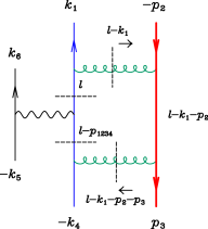
This coefficient is obtained from the cuts shown in Fig. 8,
Refer to caption
Figure 8: Diagram for the calculation of the coefficient of the scalar integral D0(k1,p2,p34;0,0,m,0)subscript𝐷0subscript𝑘1subscript𝑝2subscript𝑝3400𝑚0D_{0}(k_{1},p_{2},p_{34};0,0,m,0). The massive quark is represented by the heavy (red) line and unitarity cuts are represented by a dashed line.

where the loop momentum is subject to the conditions,

l2=0,(lk1)2=0,(lk1p2)2=m2,l12342=(lk1p2p3k4)2=0.formulae-sequencesuperscript𝑙20formulae-sequencesuperscript𝑙subscript𝑘120formulae-sequencesuperscript𝑙subscript𝑘1subscript𝑝22superscript𝑚2superscriptsubscript𝑙12342superscript𝑙subscript𝑘1subscript𝑝2subscript𝑝3subscript𝑘420l^{2}=0,\;\;(l-k_{1})^{2}=0,\;\;(l-k_{1}-p_{2})^{2}=m^{2},\;\;l_{1234}^{2}=(l-k_{1}-p_{2}-p_{3}-k_{4})^{2}=0\;. (49)

An explicit solution for l1=lk1subscript𝑙1𝑙subscript𝑘1l_{1}=l-k_{1} is given by,

l1μ=s23421|𝟐γμ|11|𝟐(𝟑+4)|1,superscriptsubscript𝑙1𝜇subscript𝑠2342quantum-operator-product12superscript𝛾𝜇1quantum-operator-product12341l_{1}^{\mu}=\frac{s_{234}}{2}\frac{\langle 1|\hbox to0.0pt{$\;\!\!\not$\hss}{{\bf 2}}\gamma^{\mu}|1\rangle}{\langle 1|\hbox to0.0pt{$\;\!\!\not$\hss}{{\bf 2}}(\hbox to0.0pt{$\;\!\!\not$\hss}{{\bf 3}}+\hbox to0.0pt{$\;\!\!\not$\hss}{4})|1\rangle}\;, (50)

which clearly satisfies the constraints in Eq. (49). From this we can also derive a useful form for the momentum l1234subscript𝑙1234l_{1234},

l1234μ=l1p2p3k4=121|𝟐(𝟐+𝟑+4)γμ(𝟐+𝟑+4)|11|𝟐(𝟑+4)|1.superscriptsubscript𝑙1234𝜇subscript𝑙1subscript𝑝2subscript𝑝3subscript𝑘412quantum-operator-product12234superscript𝛾𝜇2341quantum-operator-product12341l_{1234}^{\mu}=l_{1}-p_{2}-p_{3}-k_{4}=-\frac{1}{2}\frac{\langle 1|\hbox to0.0pt{$\;\!\!\not$\hss}{{\bf 2}}(\hbox to0.0pt{$\;\!\!\not$\hss}{\bf 2}+\hbox to0.0pt{$\;\!\!\not$\hss}{\bf 3}+\hbox to0.0pt{$\;\!\!\not$\hss}{4})\gamma^{\mu}{(\hbox to0.0pt{$\;\!\!\not$\hss}{\bf 2}+\hbox to0.0pt{$\;\!\!\not$\hss}{\bf 3}+\hbox to0.0pt{$\;\!\!\not$\hss}{4})}|1\rangle}{\langle 1|\hbox to0.0pt{$\;\!\!\not$\hss}{\bf 2}(\hbox to0.0pt{$\;\!\!\not$\hss}{\bf 3}+\hbox to0.0pt{$\;\!\!\not$\hss}{4})|1\rangle}\;. (51)

The other solution, corresponding to [l1|[1|[l_{1}|\sim[1| can be obtained from Eq. (50) by complex conjugation. We note that both of these parameterizations can be obtained from Eqs. (39) and (40) by simply making the replacements, 𝟑(𝟑+4)334\hbox to0.0pt{$\;\!\!\not$\hss}{\bf 3}\to(\hbox to0.0pt{$\;\!\!\not$\hss}{\bf 3}+\hbox to0.0pt{$\;\!\!\not$\hss}{4}) and s23s234subscript𝑠23subscript𝑠234s_{23}\to s_{234}. From these forms it is straightforward to compute the coefficients of this box.

IV.2.3 Calculation of d1|23|4subscript𝑑1234d_{1|23|4}

The cuts used to isolate this coefficient are depicted in Fig. 9. This box with massless internal lines and two opposite massive external lines is often referred to as the easy box Bern:1993kr . The heavy quark does not participate in the loop, and the loop momentum is subject to the following constraints,

l2=0,(lk1)2=0,(lk1p2p3)2=0,(lk1p2p3k4)2=0,formulae-sequencesuperscript𝑙20formulae-sequencesuperscript𝑙subscript𝑘120formulae-sequencesuperscript𝑙subscript𝑘1subscript𝑝2subscript𝑝320superscript𝑙subscript𝑘1subscript𝑝2subscript𝑝3subscript𝑘420l^{2}=0,\;\;(l-k_{1})^{2}=0,\;\;(l-k_{1}-p_{2}-p_{3})^{2}=0,\;\;(l-k_{1}-p_{2}-p_{3}-k_{4})^{2}=0,\;\; (52)
Refer to caption
Figure 9: Diagram for the calculation of the coefficient of the scalar integral D0(k1,p23,k4;0,0,0,0)subscript𝐷0subscript𝑘1subscript𝑝23subscript𝑘40000D_{0}(k_{1},p_{23},k_{4};0,0,0,0). The massive quark is represented by the heavy (red) line and unitarity cuts are represented by a dashed line.

The explicit solutions for l1=lk1subscript𝑙1𝑙subscript𝑘1l_{1}=l-k_{1} and l123=lk1p2p3subscript𝑙123𝑙subscript𝑘1subscript𝑝2subscript𝑝3l_{123}=l-k_{1}-p_{2}-p_{3} are given either by,

l1μsuperscriptsubscript𝑙1𝜇\displaystyle l_{1}^{\mu} =\displaystyle= 124|(𝟐+𝟑)γμ|14 1,12quantum-operator-product423superscript𝛾𝜇1delimited-⟨⟩41\displaystyle~{}~{}\frac{1}{2}\frac{\langle 4|{\bf(\hbox to0.0pt{$\;\!\!\not$\hss}{2}+\hbox to0.0pt{$\;\!\!\not$\hss}{3})}\gamma^{\mu}|1\rangle}{\left\langle 4\,1\right\rangle}\;,
l123μsuperscriptsubscript𝑙123𝜇\displaystyle l_{123}^{\mu} =\displaystyle= 124|γμ(𝟐+𝟑)|14 1,12quantum-operator-product4superscript𝛾𝜇231delimited-⟨⟩41\displaystyle-\frac{1}{2}\frac{\langle 4|\gamma^{\mu}{\bf(\hbox to0.0pt{$\;\!\!\not$\hss}{2}+\hbox to0.0pt{$\;\!\!\not$\hss}{3})}|1\rangle}{\left\langle 4\,1\right\rangle}\;, (53)

or by,

l1μsuperscriptsubscript𝑙1𝜇\displaystyle l_{1}^{\mu} =\displaystyle= 12[4|(𝟐+𝟑)γμ|1][4 1],12delimited-[]423superscript𝛾𝜇1delimited-[]41\displaystyle~{}~{}\frac{1}{2}\frac{[4|{\bf(\hbox to0.0pt{$\;\!\!\not$\hss}{2}+\hbox to0.0pt{$\;\!\!\not$\hss}{3})}\gamma^{\mu}|1]}{\left[4\,1\right]}\;,
l123μsuperscriptsubscript𝑙123𝜇\displaystyle l_{123}^{\mu} =\displaystyle= 12[4|γμ(𝟐+𝟑)|1][4 1].12delimited-[]4superscript𝛾𝜇231delimited-[]41\displaystyle-\frac{1}{2}\frac{[4|\gamma^{\mu}{\bf(\hbox to0.0pt{$\;\!\!\not$\hss}{2}+\hbox to0.0pt{$\;\!\!\not$\hss}{3})}|1]}{\left[4\,1\right]}\;. (54)

Both of these clearly satisfy the constraints in Eq. (52).

As an example, we will calculate the coefficient of this box integral for the spin label choice {,+}\{-,+\}. For this spin label choice it turns out that the box coefficient vanishes. The argument is quite general and may be useful in explaining the absence of the easy box in other contexts, e.g. ref. Badger:2009vh . The result for the box coefficient is calculated from,

d1|23|4(,+)=ha,hbsubscript𝑑1234subscriptsubscript𝑎subscript𝑏\displaystyle d_{1|23|4}(-,+)=\sum_{h_{a},h_{b}} A3(1q,l+q¯,l1ha)×A4(lq,l1234q¯+,5l¯+,6l)subscript𝐴3superscriptsubscript1𝑞subscriptsuperscript𝑙¯𝑞superscriptsubscript𝑙1subscript𝑎subscript𝐴4subscriptsuperscript𝑙𝑞superscriptsubscript𝑙1234¯𝑞superscriptsubscript5¯𝑙superscriptsubscript6𝑙\displaystyle A_{3}(1_{\vphantom{{\bar{q}}}{q}}^{-},-{l^{+}}_{\bar{q}},l_{1}^{h_{a}})\times A_{4}({l^{-}}_{\vphantom{{\bar{q}}}{q}},-l_{1234\;{\bar{q}}}^{+},5_{\bar{l}}^{+},6_{\vphantom{{\bar{l}}}{l}}^{-}) (55)
×A3(l1234q,4q¯+,l123hb)×A4(l1ha,2Q¯+,3Q,l123hb),absentsubscript𝐴3superscriptsubscript𝑙1234𝑞superscriptsubscript4¯𝑞superscriptsubscript𝑙123subscript𝑏subscript𝐴4superscriptsubscript𝑙1subscript𝑎superscriptsubscript2¯𝑄superscriptsubscript3𝑄superscriptsubscript𝑙123subscript𝑏\displaystyle\times A_{3}(l_{1234\;{\vphantom{{\bar{q}}}{q}}}^{-},4_{\bar{q}}^{+},-{\vphantom{{\bar{l}}}{l}}_{123}^{h_{b}})\times A_{4}(-l_{1}^{-h_{a}},2_{\bar{Q}}^{+},3_{\vphantom{{\bar{Q}}}{Q}}^{-},l_{123}^{-h_{b}})\;,

with the loop momenta fixed according to the constraints above, i.e. lμsuperscript𝑙𝜇l^{\mu} is given by either Eq. (IV.2.3) or (IV.2.3) above. From Eq. (B.1) we see that A4(l1ha,2Q¯+,3Q,l123hb)subscript𝐴4superscriptsubscript𝑙1subscript𝑎superscriptsubscript2¯𝑄superscriptsubscript3𝑄superscriptsubscript𝑙123subscript𝑏A_{4}(-l_{1}^{-h_{a}},2_{\bar{Q}}^{+},3_{\vphantom{{\bar{Q}}}{Q}}^{-},l_{123}^{-h_{b}}) vanishes for ha=hbsubscript𝑎subscript𝑏h_{a}=h_{b}. Therefore we need only consider the case ha=hbsubscript𝑎subscript𝑏h_{a}=-h_{b}. For definiteness let us consider the case ha=1,hb=1formulae-sequencesubscript𝑎1subscript𝑏1h_{a}=1,h_{b}=-1. For this case we find that,

A3(1q,l+q¯,l1+)=[ll1]2[1l][l1 1]subscript𝐴3superscriptsubscript1𝑞subscriptsuperscript𝑙¯𝑞superscriptsubscript𝑙1superscriptdelimited-[]𝑙subscript𝑙12delimited-[]1𝑙delimited-[]subscript𝑙11\displaystyle A_{3}(1_{\vphantom{{\bar{q}}}{q}}^{-},-{l^{+}}_{\bar{q}},l_{1}^{+})=\frac{{\left[l\,l_{1}\right]}^{2}}{\left[1\,l\right]\left[l_{1}\,1\right]}\quad \displaystyle\implies |l1|1,similar-toketsubscript𝑙1ket1\displaystyle|l_{1}\rangle\sim|1\rangle\;,
A3(l1234q,4q¯+,l123)=l1234l12324l1234l1234subscript𝐴3superscriptsubscript𝑙1234𝑞superscriptsubscript4¯𝑞superscriptsubscript𝑙123superscriptdelimited-⟨⟩subscript𝑙1234subscript𝑙1232delimited-⟨⟩4subscript𝑙123delimited-⟨⟩4subscript𝑙1234\displaystyle A_{3}(l_{1234\;{\vphantom{{\bar{q}}}{q}}}^{-},4_{\bar{q}}^{+},-{\vphantom{{\bar{l}}}{l}}_{123}^{-})=\frac{{\left\langle l_{1234}\,l_{123}\right\rangle}^{2}}{\left\langle 4\,l_{123}\right\rangle\left\langle 4\,l_{1234}\right\rangle}\quad \displaystyle\implies |l123]|4].\displaystyle|{\vphantom{{\bar{l}}}{l}}_{123}]\sim|4]\;. (56)

However we see that the conditions |l1|1,|l123]|4]|l_{1}\rangle\sim|1\rangle,|{\vphantom{{\bar{l}}}{l}}_{123}]\sim|4] in Eq. (IV.2.3) are not compatible with the kinematic constraints, Eqs. (IV.2.3,IV.2.3) which require either,

|l1|1andsimilar-toketsubscript𝑙1ket1and\displaystyle|l_{1}\rangle\sim|1\rangle~{}\mbox{and}~{} |l123|4,similar-toketsubscript𝑙123ket4\displaystyle|{\vphantom{{\bar{l}}}{l}}_{123}\rangle\sim|4\rangle\;,
oror\displaystyle{\rm or} |l1]|1]and\displaystyle|l_{1}]\sim|1]~{}\mbox{and}~{} |l123]|4],\displaystyle|{\vphantom{{\bar{l}}}{l}}_{123}]\sim|4]\;, (57)

respectively. The argument follows identically for the contribution ha=1,hb=+1formulae-sequencesubscript𝑎1subscript𝑏1h_{a}=-1,h_{b}=+1. Therefore for this external spin label choice {,+}\{-,+\} the box coefficient is zero. For the spin label choice {,}\{-,-\} there is a non-zero easy box coefficient because A4(l1ha,2Q¯+,3Q,l123hb)subscript𝐴4superscriptsubscript𝑙1subscript𝑎superscriptsubscript2¯𝑄superscriptsubscript3𝑄superscriptsubscript𝑙123subscript𝑏A_{4}(-l_{1}^{-h_{a}},2_{\bar{Q}}^{+},3_{\vphantom{{\bar{Q}}}{Q}}^{-},l_{123}^{-h_{b}}) no longer vanishes for ha=hbsubscript𝑎subscript𝑏h_{a}=h_{b}.

IV.3 Calculation of triangle coefficients

The leading colour amplitude receives contributions from the ten triangle scalar integrals listed in Table 2.

      Scalar integral Coefficient       Scalar integral Coefficient
1. C0(p23,k4;0,0,0)subscript𝐶0subscript𝑝23subscript𝑘4000C_{0}(p_{23},k_{4};0,0,0) c23|4subscript𝑐conditional234c_{23|4} 6. C0(k1,p23,0,0,0)subscript𝐶0subscript𝑘1subscript𝑝23000C_{0}(k_{1},p_{23},0,0,0) c1|23subscript𝑐conditional123c_{1|23}
2. C0(p12,p3;0,m,0)subscript𝐶0subscript𝑝12subscript𝑝30𝑚0C_{0}(p_{12},p_{3};0,m,0) c12|3subscript𝑐conditional123c_{12|3} 7. C0(p3,k4,m,0,0)subscript𝐶0subscript𝑝3subscript𝑘4𝑚00C_{0}(p_{3},k_{4},m,0,0) c3|4subscript𝑐conditional34c_{3|4}
3. C0(p12,p34;0,m,0)subscript𝐶0subscript𝑝12subscript𝑝340𝑚0C_{0}(p_{12},p_{34};0,m,0) c12|34subscript𝑐conditional1234c_{12|34} 8. C0(k1,p2,0,0,m)subscript𝐶0subscript𝑘1subscript𝑝200𝑚C_{0}(k_{1},p_{2},0,0,m) c1|2subscript𝑐conditional12c_{1|2}
4. C0(p2,p3;0,m,0)subscript𝐶0subscript𝑝2subscript𝑝30𝑚0C_{0}(p_{2},p_{3};0,m,0) c2|3subscript𝑐conditional23c_{2|3} 9. C0(k1,p234,0,0,0)subscript𝐶0subscript𝑘1subscript𝑝234000C_{0}(k_{1},p_{234},0,0,0) c1|234subscript𝑐conditional1234c_{1|234}
5. C0(p2,p34;0,m,0)subscript𝐶0subscript𝑝2subscript𝑝340𝑚0C_{0}(p_{2},p_{34};0,m,0) c2|34subscript𝑐conditional234c_{2|34} 10. C0(p123,k4,0,0,0)subscript𝐶0subscript𝑝123subscript𝑘4000C_{0}(p_{123},k_{4},0,0,0) c123|4subscript𝑐conditional1234c_{123|4}
Table 2: Scalar triangle integrals appearing in the leading colour amplitude A6lc(1,2,3,4)subscriptsuperscript𝐴lc61234A^{\rm lc}_{6}(1,2,3,4) and the notation used in the text to denote their coefficients.

The coefficients of Triangles 1–4 are calculated directly as detailed in the subsection below. Triangle 5 can be simply obtained by symmetry,

c2|34(h3,h2)=flip[c12|3(h2,h3)].subscript𝑐conditional234subscript3subscript2flipdelimited-[]subscript𝑐conditional123subscript2subscript3c_{2|34}(h_{3},h_{2})=-\mbox{flip}\left[c_{12|3}(-h_{2},-h_{3})\right]\;. (58)

The coefficients of the five remaining triangles are then uniquely determined by the known divergence structure Catani:2000ef of the amplitude, Eq. (36). The terms in Eq. (36) proportional to log(2k1.p2)/ϵ\log(-2k_{1}.p_{2})/\epsilon and log(2k4.p3)/ϵ\log(-2k_{4}.p_{3})/\epsilon fix two of the triangle coefficients,

c1|2subscript𝑐conditional12\displaystyle c_{1|2} =\displaystyle= (1|𝟐|1](iA6tree)+d1|2|3s23+d1|2|34s234),\displaystyle-\left(\langle\mskip-1.0mu{1}|\hbox to0.0pt{$\;\!\!\not$\hss}{\bf 2}|{1}\mskip-1.0mu]\left(-iA^{{\rm tree}}_{6}\right)+\frac{d_{1|2|3}}{s_{23}}+\frac{d_{1|2|34}}{s_{234}}\right)\;,
c3|4subscript𝑐conditional34\displaystyle c_{3|4} =\displaystyle= (4|𝟑|4](iA6tree)+d2|3|4s23+d12|3|4s123),\displaystyle-\left(\langle\mskip-1.0mu{4}|\hbox to0.0pt{$\;\!\!\not$\hss}{\bf 3}|{4}\mskip-1.0mu]\left(-iA^{{\rm tree}}_{6}\right)+\frac{d_{2|3|4}}{s_{23}}+\frac{d_{12|3|4}}{s_{123}}\right)\;, (59)

while the absence of single poles of the form log(s)/ϵ𝑠italic-ϵ\log(s)/\epsilon for s{s23,s1234,s123,s234}𝑠subscript𝑠23subscript𝑠1234subscript𝑠123subscript𝑠234s\in\{s_{23},s_{1234},s_{123},s_{234}\} requires the following relations,

c1|23subscript𝑐conditional123\displaystyle c_{1|23} =\displaystyle= 1|2+3|1](d1|2|3s231|𝟐|1]+d2|3|4s234|𝟑|4]c23|44|2+3|4]2d1|23|41|2+3|4]4|2+3|1]),\displaystyle\langle\mskip-1.0mu{1}|2+3|{1}\mskip-1.0mu]\left(\frac{d_{1|2|3}}{s_{23}\langle\mskip-1.0mu{1}|\hbox to0.0pt{$\;\!\!\not$\hss}{\bf 2}|{1}\mskip-1.0mu]}+\frac{d_{2|3|4}}{s_{23}\langle\mskip-1.0mu{4}|\hbox to0.0pt{$\;\!\!\not$\hss}{\bf 3}|{4}\mskip-1.0mu]}-\frac{c_{23|4}}{\langle\mskip-1.0mu{4}|2+3|{4}\mskip-1.0mu]}-\frac{2d_{1|23|4}}{\langle\mskip-1.0mu{1}|2+3|{4}\mskip-1.0mu]\langle\mskip-1.0mu{4}|2+3|{1}\mskip-1.0mu]}\right)\;,
c1|234subscript𝑐conditional1234\displaystyle c_{1|234} =\displaystyle= 1|2+3+4|1](d1|2|3s231|𝟐|1]+d1|2|34s2341|𝟐|1]c1|231|2+3|1]),\displaystyle\langle\mskip-1.0mu{1}|2+3+4|{1}\mskip-1.0mu]\left(\frac{d_{1|2|3}}{s_{23}\langle\mskip-1.0mu{1}|\hbox to0.0pt{$\;\!\!\not$\hss}{\bf 2}|{1}\mskip-1.0mu]}+\frac{d_{1|2|34}}{s_{234}\langle\mskip-1.0mu{1}|\hbox to0.0pt{$\;\!\!\not$\hss}{\bf 2}|{1}\mskip-1.0mu]}-\frac{c_{1|23}}{\langle\mskip-1.0mu{1}|2+3|{1}\mskip-1.0mu]}\right)\;, (60)
c123|4subscript𝑐conditional1234\displaystyle c_{123|4} =\displaystyle= 4|1+2+3|4](d12|3|4s1234|𝟑|4]+d1|2|34s2341|𝟐|1]c1|2341|2+3+4|1]+2d1|23|41|2+3|4]4|2+3|1]).\displaystyle\langle\mskip-1.0mu{4}|1+2+3|{4}\mskip-1.0mu]\left(\frac{d_{12|3|4}}{s_{123}\langle\mskip-1.0mu{4}|\hbox to0.0pt{$\;\!\!\not$\hss}{\bf 3}|{4}\mskip-1.0mu]}+\frac{d_{1|2|34}}{s_{234}\langle\mskip-1.0mu{1}|\hbox to0.0pt{$\;\!\!\not$\hss}{\bf 2}|{1}\mskip-1.0mu]}-\frac{c_{1|234}}{\langle\mskip-1.0mu{1}|2+3+4|{1}\mskip-1.0mu]}+\frac{2d_{1|23|4}}{\langle\mskip-1.0mu{1}|2+3|{4}\mskip-1.0mu]\langle\mskip-1.0mu{4}|2+3|{1}\mskip-1.0mu]}\right)\;.

These expressions are written in terms of already-calculated box and triangle coefficients, the leading order amplitude, and the other triangle coefficients discussed below.

IV.3.1 Forde method for triangle coefficients

We will calculate the coefficients of the triangle integrals using the method of Forde Forde:2007mi . Triangles 2, 3 and 4 will require a slight extension of the formalism to include one of the internal propagators with a mass. We first review the case of three massless internal momenta, shown in Fig. 10 in order to introduce our notation which differs from that of Forde.

Refer to caption
Figure 10: Triangle diagram showing the momentum parameterization. All momenta are outgoing, K1+K2+K3=0subscript𝐾1subscript𝐾2subscript𝐾30K_{1}+K_{2}+K_{3}=0.

Defining l1subscript𝑙1l_{1} and l2subscript𝑙2l_{2} as follows,

l1μ=l0μK1μ,superscriptsubscript𝑙1𝜇superscriptsubscript𝑙0𝜇superscriptsubscript𝐾1𝜇\displaystyle l_{1}^{\mu}=l_{0}^{\mu}-K_{1}^{\mu}\;, l2μ=l0μ+K2μ,superscriptsubscript𝑙2𝜇superscriptsubscript𝑙0𝜇superscriptsubscript𝐾2𝜇\displaystyle l_{2}^{\mu}=l_{0}^{\mu}+K_{2}^{\mu}\;, (61)

the cut loop momenta (li2=0),i=0,1,2formulae-sequencesuperscriptsubscript𝑙𝑖20𝑖012(l_{i}^{2}=0),i=0,1,2 may be written in the following general form,

liμ=xiK1,μ+yiK2,μ+t2K1|γμ|K2]+xiyi2tK2|γμ|K1].\displaystyle l^{\mu}_{i}=x_{i}K_{1}^{\flat,\mu}+y_{i}K_{2}^{\flat,\mu}+\frac{t}{2}\langle\mskip-1.0mu{K^{\flat}_{1}}|\gamma^{\mu}|{K^{\flat}_{2}}\mskip-1.0mu]+\frac{x_{i}y_{i}}{2t}\langle\mskip-1.0mu{K^{\flat}_{2}}|\gamma^{\mu}|{K^{\flat}_{1}}\mskip-1.0mu]\;. (62)

All momenta can be expanded in terms of massless momenta, K1superscriptsubscript𝐾1K_{1}^{\flat} and K2superscriptsubscript𝐾2K_{2}^{\flat},

K1subscript𝐾1\displaystyle K_{1} =\displaystyle= K1+S1γK2,superscriptsubscript𝐾1subscript𝑆1𝛾superscriptsubscript𝐾2\displaystyle K_{1}^{\flat}+\frac{S_{1}}{\gamma}K_{2}^{\flat}\;,
K2subscript𝐾2\displaystyle K_{2} =\displaystyle= K2+S2γK1,superscriptsubscript𝐾2subscript𝑆2𝛾superscriptsubscript𝐾1\displaystyle K_{2}^{\flat}+\frac{S_{2}}{\gamma}K_{1}^{\flat}\;,
K3subscript𝐾3\displaystyle K_{3} =\displaystyle= (1+S2γ)K1(1+S1γ)K2,1subscript𝑆2𝛾superscriptsubscript𝐾11subscript𝑆1𝛾superscriptsubscript𝐾2\displaystyle-(1+\frac{S_{2}}{\gamma})K_{1}^{\flat}-(1+\frac{S_{1}}{\gamma})K_{2}^{\flat}\;, (63)

where Si=Ki2subscript𝑆𝑖superscriptsubscript𝐾𝑖2S_{i}=K_{i}^{2} and γ=K1|K2|K1]=2K2K1\gamma=\langle\mskip-1.0mu{K_{1}^{\flat}}|K_{2}^{\flat}|{K_{1}^{\flat}}\mskip-1.0mu]=2{K_{2}^{\flat}}\cdot{K_{1}^{\flat}}. The inverse relations are,

K1,μ=K1μ(S1/γ)K2μ1(S1S2/γ2),K2,μ=K2μ(S2/γ)K1μ1(S1S2/γ2).formulae-sequencesuperscriptsubscript𝐾1𝜇subscriptsuperscript𝐾𝜇1subscript𝑆1𝛾superscriptsubscript𝐾2𝜇1subscript𝑆1subscript𝑆2superscript𝛾2superscriptsubscript𝐾2𝜇superscriptsubscript𝐾2𝜇subscript𝑆2𝛾subscriptsuperscript𝐾𝜇11subscript𝑆1subscript𝑆2superscript𝛾2\displaystyle K_{1}^{\flat,\mu}=\frac{K^{\mu}_{1}-(S_{1}/\gamma)K_{2}^{\mu}}{1-(S_{1}S_{2}/\gamma^{2})},\;\;\;\;\;K_{2}^{\flat,\mu}=\frac{K_{2}^{\mu}-(S_{2}/\gamma)K^{\mu}_{1}}{1-(S_{1}S_{2}/\gamma^{2})}\;. (64)

The dot product of K1subscript𝐾1K_{1} and K2subscript𝐾2K_{2} in Eq. (IV.3.1) produces a quadratic equation for γ𝛾\gamma, the solutions of which express γ𝛾\gamma in terms of the external momenta,

γ±=(K1K2)±Δ,Δ=(K1K2)2S1S2.formulae-sequencesubscript𝛾plus-or-minusplus-or-minussubscript𝐾1subscript𝐾2ΔΔsuperscriptsubscript𝐾1subscript𝐾22subscript𝑆1subscript𝑆2\displaystyle\gamma_{\pm}=(K_{1}\cdot K_{2})\pm\sqrt{\Delta},\;\;\;\;\;\;\Delta=(K_{1}\cdot K_{2})^{2}-S_{1}S_{2}\;. (65)

From Eq. (62) the massless vectors lisubscript𝑙𝑖l_{i} can be expressed as a linear combination of the spinor solutions for the vectors K1superscriptsubscript𝐾1K_{1}^{\flat} and K2superscriptsubscript𝐾2K_{2}^{\flat},

li|=tK1|+yiK2|,brasubscript𝑙𝑖𝑡brasuperscriptsubscript𝐾1subscript𝑦𝑖brasuperscriptsubscript𝐾2\displaystyle\langle l_{i}|=t\langle K_{1}^{\flat}|+y_{i}\langle K_{2}^{\flat}|\;, [li|=xit[K1|+[K2|.\displaystyle[l_{i}|=\frac{x_{i}}{t}[K_{1}^{\flat}|+[K_{2}^{\flat}|\;. (66)

The on-shell conditions li2=0superscriptsubscript𝑙𝑖20l_{i}^{2}=0 for i=0,1,2𝑖012i=0,1,2 allow us to derive the coefficients, xisubscript𝑥𝑖x_{i} and yisubscript𝑦𝑖y_{i},

y0=S1(γ+S2)(γ2S1S2),subscript𝑦0subscript𝑆1𝛾subscript𝑆2superscript𝛾2subscript𝑆1subscript𝑆2\displaystyle y_{0}=\frac{S_{1}\left(\gamma+S_{2}\right)}{\left(\gamma^{2}-S_{1}S_{2}\right)},\;\; x0=S2(γ+S1)(γ2S1S2),subscript𝑥0subscript𝑆2𝛾subscript𝑆1superscript𝛾2subscript𝑆1subscript𝑆2\displaystyle\;\;x_{0}=-\frac{S_{2}\left(\gamma+S_{1}\right)}{\left(\gamma^{2}-S_{1}S_{2}\right)},
y1=y0S1γ=S1S2(γ+S1)γ(γ2S1S2),subscript𝑦1subscript𝑦0subscript𝑆1𝛾subscript𝑆1subscript𝑆2𝛾subscript𝑆1𝛾superscript𝛾2subscript𝑆1subscript𝑆2\displaystyle y_{1}=y_{0}-\frac{S_{1}}{\gamma}=\frac{S_{1}S_{2}\left(\gamma+S_{1}\right)}{\gamma(\gamma^{2}-S_{1}S_{2})},\;\; x1=x01=γ(γ+S2)γ2S1S2,subscript𝑥1subscript𝑥01𝛾𝛾subscript𝑆2superscript𝛾2subscript𝑆1subscript𝑆2\displaystyle\;\;x_{1}=x_{0}-1=-\frac{\gamma(\gamma+S_{2})}{\gamma^{2}-S_{1}S_{2}},
y2=y0+1=γ(γ+S1)γ2S1S2,subscript𝑦2subscript𝑦01𝛾𝛾subscript𝑆1superscript𝛾2subscript𝑆1subscript𝑆2\displaystyle y_{2}=y_{0}+1=\frac{\gamma(\gamma+S_{1})}{\gamma^{2}-S_{1}S_{2}},\;\; x2=x0+S2γ=S1S2(γ+S2)γ(γ2S1S2).subscript𝑥2subscript𝑥0subscript𝑆2𝛾subscript𝑆1subscript𝑆2𝛾subscript𝑆2𝛾superscript𝛾2subscript𝑆1subscript𝑆2\displaystyle\;\;x_{2}=x_{0}+\frac{S_{2}}{\gamma}=-\frac{S_{1}S_{2}\left(\gamma+S_{2}\right)}{\gamma(\gamma^{2}-S_{1}S_{2})}\;. (67)

The spinor products can be expressed as follows,

[ll1]delimited-[]𝑙subscript𝑙1\displaystyle\left[ll_{1}\right] =\displaystyle= x1x0t[K2K1]=1t[K2K1],subscript𝑥1subscript𝑥0𝑡delimited-[]subscriptsuperscript𝐾2subscriptsuperscript𝐾11𝑡delimited-[]subscriptsuperscript𝐾2subscriptsuperscript𝐾1\displaystyle\frac{x_{1}-x_{0}}{t}[K^{\flat}_{2}K^{\flat}_{1}]=-\frac{1}{t}[K^{\flat}_{2}K^{\flat}_{1}],
ll1delimited-⟨⟩𝑙subscript𝑙1\displaystyle\left\langle l\,l_{1}\right\rangle =\displaystyle= t(y1y0)K1K2=tS1γK1K2,𝑡subscript𝑦1subscript𝑦0delimited-⟨⟩subscriptsuperscript𝐾1subscriptsuperscript𝐾2𝑡subscript𝑆1𝛾delimited-⟨⟩subscriptsuperscript𝐾1subscriptsuperscript𝐾2\displaystyle t(y_{1}-y_{0})\left\langle K^{\flat}_{1}\,K^{\flat}_{2}\right\rangle=-\frac{tS_{1}}{\gamma}\left\langle K^{\flat}_{1}\,K^{\flat}_{2}\right\rangle,
[ll2]delimited-[]𝑙subscript𝑙2\displaystyle\left[ll_{2}\right] =\displaystyle= x2x0t[K2K1]=S2γt[K2K1],subscript𝑥2subscript𝑥0𝑡delimited-[]subscriptsuperscript𝐾2subscriptsuperscript𝐾1subscript𝑆2𝛾𝑡delimited-[]subscriptsuperscript𝐾2subscriptsuperscript𝐾1\displaystyle\frac{x_{2}-x_{0}}{t}[K^{\flat}_{2}K^{\flat}_{1}]=\frac{S_{2}}{\gamma t}[K^{\flat}_{2}K^{\flat}_{1}],
ll2delimited-⟨⟩𝑙subscript𝑙2\displaystyle\left\langle l\,l_{2}\right\rangle =\displaystyle= t(y2y0)K1K2=tK1K2,𝑡subscript𝑦2subscript𝑦0delimited-⟨⟩subscriptsuperscript𝐾1subscriptsuperscript𝐾2𝑡delimited-⟨⟩subscriptsuperscript𝐾1subscriptsuperscript𝐾2\displaystyle t(y_{2}-y_{0})\left\langle K^{\flat}_{1}\,K^{\flat}_{2}\right\rangle=t\left\langle K^{\flat}_{1}\,K^{\flat}_{2}\right\rangle,
[l1l2]delimited-[]subscript𝑙1subscript𝑙2\displaystyle\left[l_{1}l_{2}\right] =\displaystyle= x2x1t[K2K1]=1t(1+S2γ)[K2K1],subscript𝑥2subscript𝑥1𝑡delimited-[]subscriptsuperscript𝐾2subscriptsuperscript𝐾11𝑡1subscript𝑆2𝛾delimited-[]subscriptsuperscript𝐾2subscriptsuperscript𝐾1\displaystyle\frac{x_{2}-x_{1}}{t}[K^{\flat}_{2}K^{\flat}_{1}]=\frac{1}{t}\left(1+\frac{S_{2}}{\gamma}\right)[K^{\flat}_{2}K^{\flat}_{1}],
l1l2delimited-⟨⟩subscript𝑙1subscript𝑙2\displaystyle\left\langle l_{1}\,l_{2}\right\rangle =\displaystyle= t(y2y1)K1K2=t(1+S1γ)K1K2.𝑡subscript𝑦2subscript𝑦1delimited-⟨⟩subscriptsuperscript𝐾1subscriptsuperscript𝐾2𝑡1subscript𝑆1𝛾delimited-⟨⟩subscriptsuperscript𝐾1subscriptsuperscript𝐾2\displaystyle t(y_{2}-y_{1})\left\langle K^{\flat}_{1}\,K^{\flat}_{2}\right\rangle=t\left(1+\frac{S_{1}}{\gamma}\right)\left\langle K^{\flat}_{1}\,K^{\flat}_{2}\right\rangle. (68)

Turning now to the case where the propagator with momentum l2subscript𝑙2l_{2} has a mass, we have that l02=l12=0superscriptsubscript𝑙02superscriptsubscript𝑙120l_{0}^{2}=l_{1}^{2}=0 and l22=m2superscriptsubscript𝑙22superscript𝑚2l_{2}^{2}=m^{2}. Since l2subscript𝑙2l_{2} is no longer massless it does not have an expansion of the form Eq. (66). The results for the coefficients in the expansion defined in Eq. (66) for l0subscript𝑙0l_{0} and l1subscript𝑙1l_{1} are,

y0=S1(γ+S2m2)(γ2S1S2),subscript𝑦0subscript𝑆1𝛾subscript𝑆2superscript𝑚2superscript𝛾2subscript𝑆1subscript𝑆2\displaystyle y_{0}=\frac{S_{1}\left(\gamma+S_{2}-m^{2}\right)}{\left(\gamma^{2}-S_{1}S_{2}\right)},\;\; x0=γm2S2(γ+S1)(γ2S1S2),subscript𝑥0𝛾superscript𝑚2subscript𝑆2𝛾subscript𝑆1superscript𝛾2subscript𝑆1subscript𝑆2\displaystyle\;\;x_{0}=\frac{\gamma m^{2}-S_{2}\left(\gamma+S_{1}\right)}{\left(\gamma^{2}-S_{1}S_{2}\right)},
y1=y0S1γ=S1(S2(1+(S1/γ))m2)γ2S1S2,subscript𝑦1subscript𝑦0subscript𝑆1𝛾subscript𝑆1subscript𝑆21subscript𝑆1𝛾superscript𝑚2superscript𝛾2subscript𝑆1subscript𝑆2\displaystyle y_{1}=y_{0}-\frac{S_{1}}{\gamma}=\frac{S_{1}\left(S_{2}\left(1+(S_{1}/\gamma)\right)-m^{2}\right)}{\gamma^{2}-S_{1}S_{2}},\;\; x1=x01=γm2γ(S2+γ)γ2S1S2.subscript𝑥1subscript𝑥01𝛾superscript𝑚2𝛾subscript𝑆2𝛾superscript𝛾2subscript𝑆1subscript𝑆2\displaystyle\;\;x_{1}=x_{0}-1=\frac{\gamma m^{2}-\gamma(S_{2}+\gamma)}{\gamma^{2}-S_{1}S_{2}}\;. (69)
Refer to caption
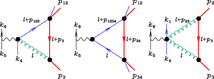
Figure 11: Diagrams for the calculation of the coefficients of the scalar integrals C0(p12,p3;0,m,0)subscript𝐶0subscript𝑝12subscript𝑝30𝑚0C_{0}(p_{12},p_{3};0,m,0), C0(p12,p34;0,m,0)subscript𝐶0subscript𝑝12subscript𝑝340𝑚0C_{0}(p_{12},p_{34};0,m,0) and C0(p2,p3;0,m,0)subscript𝐶0subscript𝑝2subscript𝑝30𝑚0C_{0}(p_{2},p_{3};0,m,0). The massive quark is represented by the heavy (red) line. The momenta on the external lines are all outgoing.

With these results in hand we can then compute the coefficients for triangles 2–4 with the loop momentum assignments as shown in Figure 11 by making the replacements:

  • Triangle 2: K1=p123subscript𝐾1subscript𝑝123K_{1}=-p_{123}, K2=p3subscript𝐾2subscript𝑝3K_{2}=p_{3}.

  • Triangle 3: K1=p1234subscript𝐾1subscript𝑝1234K_{1}=-p_{1234}, K2=p34subscript𝐾2subscript𝑝34K_{2}=p_{34}.

  • Triangle 4: K1=p23subscript𝐾1subscript𝑝23K_{1}=-p_{23}, K2=p3subscript𝐾2subscript𝑝3K_{2}=p_{3}.

For the case of triangles 2 and 4, we see that the coefficients are particularly simple since S2=m2subscript𝑆2superscript𝑚2S_{2}=m^{2}.

We shall sketch the calculation of the coefficient of triangle 4 because it is the simplest. We have S1=p232=s23subscript𝑆1superscriptsubscript𝑝232subscript𝑠23S_{1}=p_{23}^{2}=s_{23} and S2=p32=m2subscript𝑆2superscriptsubscript𝑝32superscript𝑚2S_{2}=p_{3}^{2}=m^{2} and hence see that,

γ±=K1K2±(K1K2)2S1S2=βs23.subscript𝛾plus-or-minusplus-or-minussubscript𝐾1subscript𝐾2superscriptsubscript𝐾1subscript𝐾22subscript𝑆1subscript𝑆2subscript𝛽minus-or-plussubscript𝑠23\gamma_{\pm}=K_{1}\cdot K_{2}\pm\sqrt{(K_{1}\cdot K_{2})^{2}-S_{1}S_{2}}=-\beta_{\mp}s_{23}\;. (70)

The lightlike momenta, Eq. (64), for the two solutions for γ𝛾\gamma reduce to,

K1=k2,K2=β+k3,forγ=γ=β+s23,y0=1β,x0=ββ,formulae-sequenceformulae-sequencesubscriptsuperscript𝐾1subscript𝑘2formulae-sequencesubscriptsuperscript𝐾2subscript𝛽subscript𝑘3for𝛾subscript𝛾subscript𝛽subscript𝑠23formulae-sequencesubscript𝑦01𝛽subscript𝑥0subscript𝛽𝛽\displaystyle K^{\flat}_{1}=-k_{2}\;,\quad K^{\flat}_{2}=\beta_{+}k_{3}\;,\quad{\rm for}~{}\gamma=\gamma_{-}=-\beta_{+}s_{23},\;y_{0}=-\frac{1}{\beta},\;x_{0}=-\frac{\beta_{-}}{\beta}\;,
K1=k3,K2=βk2,forγ=γ+=βs23,y0=+1β,x0=+β+β.formulae-sequenceformulae-sequencesubscriptsuperscript𝐾1subscript𝑘3formulae-sequencesubscriptsuperscript𝐾2subscript𝛽subscript𝑘2for𝛾subscript𝛾subscript𝛽subscript𝑠23formulae-sequencesubscript𝑦01𝛽subscript𝑥0subscript𝛽𝛽\displaystyle K^{\flat}_{1}=-k_{3}\;,\quad K^{\flat}_{2}=\beta_{-}k_{2}\;,\quad{\rm for}~{}\gamma=\gamma_{+}=-\beta_{-}s_{23},\;y_{0}=+\frac{1}{\beta},\;x_{0}=+\frac{\beta_{+}}{\beta}\;. (71)

Using these assignments we find that the formulae for the coefficients of this triangle are relatively compact. For example, for the {,+}\{-,+\} spin labels the result is,

c2|3(,+)=12s56[{[4 5]s123(β1 326|(1+2)|3]1 2β+21 2[1 2]26|(1+2)|3]β[1 3]2\displaystyle c_{2|3}(-,+)=\frac{1}{2s_{56}}\Bigg{[}\Biggl{\{}\frac{\left[4\,5\right]}{s_{123}}\Bigl{(}-\frac{\beta_{-}\left\langle 1\,3\right\rangle^{2}\langle\mskip-1.0mu{6}|(1+2)|{3}\mskip-1.0mu]}{\left\langle 1\,2\right\rangle}-\frac{\beta_{+}^{2}\left\langle 1\,2\right\rangle\left[1\,2\right]^{2}\langle\mskip-1.0mu{6}|(1+2)|{3}\mskip-1.0mu]}{\beta\left[1\,3\right]^{2}}
+β+β1 2[1 2]6|(1+3)|2]β[1 3]β+β1 3[1 2]6|(1+2)|3]β[1 3]\displaystyle+\frac{\beta_{+}\beta_{-}\left\langle 1\,2\right\rangle\left[1\,2\right]\langle\mskip-1.0mu{6}|(1+3)|{2}\mskip-1.0mu]}{\beta\left[1\,3\right]}-\frac{\beta_{+}\beta_{-}\left\langle 1\,3\right\rangle\left[1\,2\right]\langle\mskip-1.0mu{6}|(1+2)|{3}\mskip-1.0mu]}{\beta\left[1\,3\right]}
+(β2ββ+β+4ββ+2)β1 36|(1+3)|2])+β1 31 6[4 5]1 2\displaystyle+\frac{(\beta^{2}-\beta_{-}\beta_{+}\beta+4\beta_{-}\beta_{+}^{2})}{\beta}\left\langle 1\,3\right\rangle\langle\mskip-1.0mu{6}|(1+3)|{2}\mskip-1.0mu]\Bigr{)}+\frac{\beta_{-}\left\langle 1\,3\right\rangle\left\langle 1\,6\right\rangle\left[4\,5\right]}{\left\langle 1\,2\right\rangle}
β+22 34|(2+3)|5]6|(1+2)|3]β2 42[1 3]+β+3|(2+4)|5]6|(1+2)|3]2 4[1 3]}{flip}].\displaystyle-\frac{\beta_{+}^{2}\left\langle 2\,3\right\rangle\langle\mskip-1.0mu{4}|(2+3)|{5}\mskip-1.0mu]\langle\mskip-1.0mu{6}|(1+2)|{3}\mskip-1.0mu]}{\beta\left\langle 2\,4\right\rangle^{2}\left[1\,3\right]}+\frac{\beta_{+}\langle\mskip-1.0mu{3}|(2+4)|{5}\mskip-1.0mu]\langle\mskip-1.0mu{6}|(1+2)|{3}\mskip-1.0mu]}{\left\langle 2\,4\right\rangle\left[1\,3\right]}\Biggr{\}}-\Biggl{\{}\mbox{flip}\Biggr{\}}\Bigg{]}\;. (72)

IV.4 Calculation of bubble and tadpole coefficients

The bubble integrals present in the leading colour amplitude are shown in Table 3.

      Scalar integral Coefficient       Scalar integral Coefficient
1. B0(p1234;0,0)subscript𝐵0subscript𝑝123400B_{0}(p_{1234};0,0) b1234subscript𝑏1234b_{1234} 4. B0(p12;0,m)subscript𝐵0subscript𝑝120𝑚B_{0}(p_{12};0,m) b12subscript𝑏12b_{12}
2. B0(p23;0,0)subscript𝐵0subscript𝑝2300B_{0}(p_{23};0,0) b23subscript𝑏23b_{23} 5. B0(p34;0,m)subscript𝐵0subscript𝑝340𝑚B_{0}(p_{34};0,m) b34subscript𝑏34b_{34}
3. B0(p123;0,0)subscript𝐵0subscript𝑝12300B_{0}(p_{123};0,0) b123subscript𝑏123b_{123} 6. B0(p234;0,0)subscript𝐵0subscript𝑝23400B_{0}(p_{234};0,0) b234subscript𝑏234b_{234}
      B0(p2;0,m)subscript𝐵0subscript𝑝20𝑚B_{0}(p_{2};0,m) b2subscript𝑏2b_{2}       A0(m)subscript𝐴0𝑚A_{0}(m) a𝑎a
Table 3: Scalar bubble and tadpole integrals appearing in the leading colour amplitude A6lc(1,2,3,4)subscriptsuperscript𝐴lc61234A^{\rm lc}_{6}(1,2,3,4) and the notation used in the text to denote their coefficients.

The coefficients of bubbles 1–4 are computed by using the method of spinor integration Cachazo:2004kj ; Britto:2005ha ; Britto:2006sj . This is straightforward to apply for bubbles 1–3 but requires a small modification for bubble 4 due to the effect of the massive propagator. The modified method is described in the subsection below. Coefficients of the bubble integrals 5 and 6 are then obtained by symmetry,

b34(h3,h2)subscript𝑏34subscript3subscript2\displaystyle b_{34}(h_{3},h_{2}) =\displaystyle= flip[b12(h2,h3)],flipdelimited-[]subscript𝑏12subscript2subscript3\displaystyle-\mbox{flip}\left[b_{12}(-h_{2},-h_{3})\right]\;,
b234(h3,h2)subscript𝑏234subscript3subscript2\displaystyle b_{234}(h_{3},h_{2}) =\displaystyle= flip[b123(h2,h3)],flipdelimited-[]subscript𝑏123subscript2subscript3\displaystyle-\mbox{flip}\left[b_{123}(-h_{2},-h_{3})\right]\;, (73)

All occurrences of B0(p3;0,m)subscript𝐵0subscript𝑝30𝑚B_{0}(p_{3};0,m) have been replaced by B0(p2;0,m)subscript𝐵0subscript𝑝20𝑚B_{0}(p_{2};0,m), so we only need to determine the coefficient b2subscript𝑏2b_{2}. A linear combination of the coefficient b2subscript𝑏2b_{2} and a𝑎a is determined from the known form of the single pole in ϵitalic-ϵ\epsilon, (i.e. the single pole with no associated logarithm in the expansion of Eq. (36)),

b2+m2a=83(i)A6treeb123b234b23b1234b12b34.subscript𝑏2superscript𝑚2𝑎83𝑖subscriptsuperscript𝐴tree6subscript𝑏123subscript𝑏234subscript𝑏23subscript𝑏1234subscript𝑏12subscript𝑏34b_{2}+m^{2}a=\frac{8}{3}(-i)A^{{\rm tree}}_{6}-b_{123}-b_{234}-b_{23}-b_{1234}-b_{12}-b_{34}\;. (74)

Eq. (74) is sufficient to fix the poles and the logarithms, but since,

A0(m)/m2subscript𝐴0𝑚superscript𝑚2\displaystyle A_{0}(m)/m^{2} =\displaystyle= (μ2m2)ϵ(1ϵ+1),superscriptsuperscript𝜇2superscript𝑚2italic-ϵ1italic-ϵ1\displaystyle\Big{(}\frac{\mu^{2}}{m^{2}}\Big{)}^{\epsilon}\Big{(}\frac{1}{\epsilon}+1\Big{)}\;,
B0(p2;0,m)subscript𝐵0subscript𝑝20𝑚\displaystyle B_{0}(p_{2};0,m) =\displaystyle= (μ2m2)ϵ(1ϵ+2),superscriptsuperscript𝜇2superscript𝑚2italic-ϵ1italic-ϵ2\displaystyle\Big{(}\frac{\mu^{2}}{m^{2}}\Big{)}^{\epsilon}\Big{(}\frac{1}{\epsilon}+2\Big{)}\;, (75)

it leaves the constant term undetermined. In order to separately fix the coefficients a𝑎a and b2subscript𝑏2b_{2} we perform a direct Feynman diagram computation of the tadpole coefficient a𝑎a to find,

a(,+)𝑎\displaystyle a(-,+) =\displaystyle= 0,0\displaystyle 0\;,
a(+,)𝑎\displaystyle a(+,-) =\displaystyle= 0,0\displaystyle 0\;,
m2a(,)superscript𝑚2𝑎\displaystyle m^{2}a(-,-) =\displaystyle= 12(i)A6tree(1q,2Q¯,3Q,4q¯+,5¯+,6),12𝑖subscriptsuperscript𝐴tree6superscriptsubscript1𝑞superscriptsubscript2¯𝑄superscriptsubscript3𝑄superscriptsubscript4¯𝑞superscriptsubscript5¯superscriptsubscript6\displaystyle\frac{1}{2}(-i)A^{{\rm tree}}_{6}(1_{\vphantom{{\bar{q}}}{q}}^{-},2_{\bar{Q}}^{-},3_{\vphantom{{\bar{Q}}}{Q}}^{-},4_{\bar{q}}^{+},5_{\overline{\ell}}^{+},6_{\ell}^{-})\;,
m2a(+,+)superscript𝑚2𝑎\displaystyle m^{2}a(+,+) =\displaystyle= 12(i)A6tree(1q,2Q¯+,3Q+,4q¯+,5¯+,6).12𝑖subscriptsuperscript𝐴tree6superscriptsubscript1𝑞superscriptsubscript2¯𝑄superscriptsubscript3𝑄superscriptsubscript4¯𝑞superscriptsubscript5¯superscriptsubscript6\displaystyle\frac{1}{2}(-i)A^{{\rm tree}}_{6}(1_{\vphantom{{\bar{q}}}{q}}^{-},2_{\bar{Q}}^{+},3_{\vphantom{{\bar{Q}}}{Q}}^{+},4_{\bar{q}}^{+},5_{\overline{\ell}}^{+},6_{\ell}^{-})\;. (76)

These results for a𝑎a are valid in any covariant gauge.

IV.4.1 Bubble integral with one massive propagator

To set up the formalism we consider the scalar bubble integral with one massive propagator, as shown in Fig. 12 (bubbles 4 and 5 are of this type).
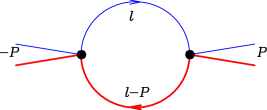
Refer to caption
Figure 12: Diagram for the calculation of the coefficient of the scalar integral B0(P;0,m)subscript𝐵0𝑃0𝑚B_{0}(P;0,m). The massive quark is represented by the heavy (red) line. The momenta on the external lines are all outgoing.

The evaluation of the coefficient of this bubble integral starts from the identity,

d4lδ(+)(l2)δ(+)((lP)2m2)=0tdtldl[ldl]δ(P2m2tl|P|l]),\int d^{4}l\,\delta^{(+)}(l^{2})\delta^{(+)}((l-P)^{2}-m^{2})=\int_{0}^{\infty}tdt\int\left\langle l\,dl\right\rangle\left[l\,dl\right]\delta(P^{2}-m^{2}-t\langle\mskip-1.0mu{l}|P|{l}\mskip-1.0mu])\;, (77)

so that the formalism follows through as in the massless case, except that t𝑡t is now frozen at the value,

t=P2m2l|P|l].𝑡superscript𝑃2superscript𝑚2delimited-⟨]𝑙𝑃𝑙t=\frac{P^{2}-m^{2}}{\langle\mskip-1.0mu{l}|P|{l}\mskip-1.0mu]}\;. (78)

The discontinuity of the scalar integral is given by,

ΔI2(P,m)Δsubscript𝐼2𝑃𝑚\displaystyle\Delta I_{2}(P,m) =\displaystyle= d4lδ(+)(l2)δ(+)((lP)2m2)superscript𝑑4𝑙superscript𝛿superscript𝑙2superscript𝛿superscript𝑙𝑃2superscript𝑚2\displaystyle\int d^{4}l\,\delta^{(+)}(l^{2})\delta^{(+)}((l-P)^{2}-m^{2}) (79)
=\displaystyle= ldl[ldl]l|P|l](P2m2l|P|l])delimited-⟨⟩𝑙𝑑𝑙delimited-[]𝑙𝑑𝑙delimited-⟨]𝑙𝑃𝑙superscript𝑃2superscript𝑚2delimited-⟨]𝑙𝑃𝑙\displaystyle\int\frac{\left\langle l\,dl\right\rangle\left[l\,dl\right]}{\langle\mskip-1.0mu{l}|P|{l}\mskip-1.0mu]}\left(\frac{P^{2}-m^{2}}{\langle\mskip-1.0mu{l}|P|{l}\mskip-1.0mu]}\right)
=\displaystyle= (P2m2)ldl[ηl]l|P|η]l|P|l].\displaystyle(P^{2}-m^{2})\int\frac{\left\langle l\,dl\right\rangle\left[\eta\,l\right]}{\langle\mskip-1.0mu{l}|P|{\eta}\mskip-1.0mu]\langle\mskip-1.0mu{l}|P|{l}\mskip-1.0mu]}\;.

Using the standard formula Cachazo:2004kj ; Britto:2005ha we can express the integrand as a total derivative, and perform one of the spinor integrations,

[ldl]([ηl]nl|P|l]n+2)=[dll](1n+11l|P|η][ηl]n+1l|P|l]n+1).\left[l\,dl\right]\left(\frac{\left[\eta\,l\right]^{n}}{\langle l|P|l]^{n+2}}\right)=\left[dl\,\partial_{l}\right]\left(\frac{1}{n+1}\frac{1}{\langle l|P|\eta]}\frac{\left[\eta\,l\right]^{n+1}}{\langle l|P|l]^{n+1}}\right)\;. (80)

We obtain,

ΔI2(P,m)=(P2m2)ldl[ηl]l|P|η]l|P|l],\Delta I_{2}(P,m)=(P^{2}-m^{2})\int\frac{\left\langle l\,dl\right\rangle\left[\eta\,l\right]}{\langle\mskip-1.0mu{l}|P|{\eta}\mskip-1.0mu]\langle\mskip-1.0mu{l}|P|{l}\mskip-1.0mu]}\;, (81)

where η𝜂\eta is an arbitrary massless momentum, We perform the final integral over ldldelimited-⟨⟩𝑙𝑑𝑙\left\langle l\,dl\right\rangle by inspecting the residues of the pole in the integrand when l|=[η|P\langle l|=[\eta|P to find,

ΔI2(P,m)Δsubscript𝐼2𝑃𝑚\displaystyle\Delta I_{2}(P,m) =\displaystyle= (P2m2)[η|P|ηP2η|P|η]\displaystyle-(P^{2}-m^{2})\frac{[\mskip-1.0mu{\eta}|P|{\eta}\mskip-1.0mu\rangle}{P^{2}\langle\mskip-1.0mu{\eta}|P|{\eta}\mskip-1.0mu]} (82)
=\displaystyle= (P2m2P2).superscript𝑃2superscript𝑚2superscript𝑃2\displaystyle-\left(\frac{P^{2}-m^{2}}{P^{2}}\right)\;. (83)

So, in contrast to the massless case, when applying the spinor integration approach an additional rescaling factor of P2/(P2m2)superscript𝑃2superscript𝑃2superscript𝑚2P^{2}/(P^{2}-m^{2}) must be applied in order to obtain the coefficient of the scalar bubble integral.

IV.5 Calculation of the rational terms

The purely rational terms are calculated using a traditional Feynman diagram approach, with tensor integrals handled using Passarino-Veltman reduction Passarino:1978jh . This might seem like a retrograde step, ineluctably leading to the algebraic complexity that we have been trying to avoid in this amplitude calculation. However two details of our particular case make it quite simple.

First, in the calculation of the rational part we only need to consider diagrams that violate the cut-constructibility condition Bern:1994cg . This states that if n𝑛n-point integrals (n>2𝑛2n>2) have at most n2𝑛2n-2 powers of the loop momentum in the numerator of the integrand, and the two-point integrals have at most one power of the loop momentum, they will be cut-constructible. For our particular calculation the pentagon diagrams are all cut-constructible, and, in leading colour, there is only one box diagram, shown in Fig. 13, which is not cut-constructible and hence gives a rational part. The calculation of the rational parts from lower point diagrams, n=3,2𝑛32n=3,2 does not lead to great algebraic complexity.
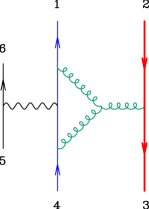
Refer to caption
Figure 13: The box diagram contributing to the rational part in leading colour.

Second, the rational terms are generated by terms in the Passarino-Veltman decomposition that involve the metric tensor, gμνsuperscript𝑔𝜇𝜈g^{\mu\nu}. Therefore any terms that are not proportional to gμνsuperscript𝑔𝜇𝜈g^{\mu\nu} may be discarded at an early stage of the computation.

The results for the rational terms turn out to be quite simple. For the {,+}\{-,+\} case we find,

Rlc(1q,2Q¯+,3Q,4q¯+,5¯+,6)=29(i)A6tree(1q,2Q¯+,3Q,4q¯+,5¯+,6)superscript𝑅lcsuperscriptsubscript1𝑞superscriptsubscript2¯𝑄superscriptsubscript3𝑄superscriptsubscript4¯𝑞superscriptsubscript5¯superscriptsubscript629𝑖subscriptsuperscript𝐴tree6superscriptsubscript1𝑞superscriptsubscript2¯𝑄superscriptsubscript3𝑄superscriptsubscript4¯𝑞superscriptsubscript5¯superscriptsubscript6\displaystyle R^{\rm lc}(1_{\vphantom{{\bar{q}}}{q}}^{-},2_{\bar{Q}}^{+},3_{\vphantom{{\bar{Q}}}{Q}}^{-},4_{\bar{q}}^{+},5_{\overline{\ell}}^{+},6_{\ell}^{-})=-\frac{2}{9}(-i)A^{\rm tree}_{6}(1_{\vphantom{{\bar{q}}}{q}}^{-},2_{\bar{Q}}^{+},3_{\vphantom{{\bar{Q}}}{Q}}^{-},4_{\bar{q}}^{+},5_{\overline{\ell}}^{+},6_{\ell}^{-}) (84)
+\displaystyle+ {1 62s56[1 3[1 5][1 2]1|(2+3)|1]4|(2+3)|1]1 3[1 5]s231|(2+3+4)|1](s234[1 2]4|(2+3)|1]+[2 4])\displaystyle\Bigg{\{}\frac{\left\langle 1\,6\right\rangle}{2s_{56}}\,\Bigg{[}\frac{\left\langle 1\,3\right\rangle\left[1\,5\right]\left[1\,2\right]}{\langle\mskip-1.0mu{1}|(2+3)|{1}\mskip-1.0mu]\langle\mskip-1.0mu{4}|(2+3)|{1}\mskip-1.0mu]}-\frac{\left\langle 1\,3\right\rangle\left[1\,5\right]}{s_{23}\langle\mskip-1.0mu{1}|(2+3+4)|{1}\mskip-1.0mu]}\Big{(}\frac{s_{234}\left[1\,2\right]}{\langle\mskip-1.0mu{4}|(2+3)|{1}\mskip-1.0mu]}+\left[2\,4\right]\Big{)}
+\displaystyle+ [2 4]s234([2 5][2 3]3 4[4 5]4|(2+3)|4])]}{flip},\displaystyle\frac{\left[2\,4\right]}{s_{234}}\Big{(}\frac{\left[2\,5\right]}{\left[2\,3\right]}-\frac{\left\langle 3\,4\right\rangle\left[4\,5\right]}{\langle\mskip-1.0mu{4}|(2+3)|{4}\mskip-1.0mu]}\Big{)}\Bigg{]}\Bigg{\}}-\Bigg{\{}{\rm flip}\Bigg{\}}\;,

where the flip operation is defined in Eq. (27). The contribution for the opposite spin labels on the heavy quark line is simply related to this one,

Rlc(1q,2Q¯,3Q+,4q¯+,5¯+,6)=Rlc(1q,3Q¯+,2Q,4q¯+,5¯+,6).superscript𝑅lcsuperscriptsubscript1𝑞superscriptsubscript2¯𝑄superscriptsubscript3𝑄superscriptsubscript4¯𝑞superscriptsubscript5¯superscriptsubscript6superscript𝑅lcsuperscriptsubscript1𝑞superscriptsubscript3¯𝑄superscriptsubscript2𝑄superscriptsubscript4¯𝑞superscriptsubscript5¯superscriptsubscript6R^{\rm lc}(1_{\vphantom{{\bar{q}}}{q}}^{-},2_{\bar{Q}}^{-},3_{\vphantom{{\bar{Q}}}{Q}}^{+},4_{\bar{q}}^{+},5_{\overline{\ell}}^{+},6_{\ell}^{-})=R^{\rm lc}(1_{\vphantom{{\bar{q}}}{q}}^{-},3_{\bar{Q}}^{+},2_{\vphantom{{\bar{Q}}}{Q}}^{-},4_{\bar{q}}^{+},5_{\overline{\ell}}^{+},6_{\ell}^{-})\;. (85)

For the {,}\{-,-\} spin labels the result is,

Rlc(1q,2Q¯,3Q,4q¯+,5¯+,6)=29(i)A6tree(1q,2Q¯,3Q,4q¯+,5¯+,6)superscript𝑅lcsuperscriptsubscript1𝑞superscriptsubscript2¯𝑄superscriptsubscript3𝑄superscriptsubscript4¯𝑞superscriptsubscript5¯superscriptsubscript629𝑖subscriptsuperscript𝐴tree6superscriptsubscript1𝑞superscriptsubscript2¯𝑄superscriptsubscript3𝑄superscriptsubscript4¯𝑞superscriptsubscript5¯superscriptsubscript6\displaystyle R^{\rm lc}(1_{\vphantom{{\bar{q}}}{q}}^{-},2_{\bar{Q}}^{-},3_{\vphantom{{\bar{Q}}}{Q}}^{-},4_{\bar{q}}^{+},5_{\overline{\ell}}^{+},6_{\ell}^{-})=-\frac{2}{9}(-i)A^{\rm tree}_{6}(1_{\vphantom{{\bar{q}}}{q}}^{-},2_{\bar{Q}}^{-},3_{\vphantom{{\bar{Q}}}{Q}}^{-},4_{\bar{q}}^{+},5_{\overline{\ell}}^{+},6_{\ell}^{-})
+\displaystyle+ 𝒩({1 62s56[[1 5]1|2+3+4|1]s23(s234(1|2|1]1|3|1])4|2+3|1](1|2|4]1|3|4]))\displaystyle{\cal N}_{--}\Bigg{(}\Biggl{\{}\frac{\left\langle 1\,6\right\rangle}{2s_{56}}\,\Biggl{[}\frac{\left[1\,5\right]}{\langle\mskip-1.0mu{1}|2+3+4|{1}\mskip-1.0mu]s_{23}}\Big{(}\frac{s_{234}(\langle\mskip-1.0mu{1}|2|{1}\mskip-1.0mu]-\langle\mskip-1.0mu{1}|3|{1}\mskip-1.0mu])}{\langle\mskip-1.0mu{4}|2+3|{1}\mskip-1.0mu]}-(\langle\mskip-1.0mu{1}|2|{4}\mskip-1.0mu]-\langle\mskip-1.0mu{1}|3|{4}\mskip-1.0mu])\Big{)}
\displaystyle- (1|2|1]1|3|1])1|2+3|1]([1 5]4|2+3|1]+[4 5]s23)]}+{flip}),\displaystyle\frac{(\langle\mskip-1.0mu{1}|2|{1}\mskip-1.0mu]-\langle\mskip-1.0mu{1}|3|{1}\mskip-1.0mu])}{\langle\mskip-1.0mu{1}|2+3|{1}\mskip-1.0mu]}\Big{(}\frac{\left[1\,5\right]}{\langle\mskip-1.0mu{4}|2+3|{1}\mskip-1.0mu]}+\frac{\left[4\,5\right]}{s_{23}}\Big{)}\Biggr{]}\Bigg{\}}+\Bigg{\{}{\rm flip}\Bigg{\}}\Bigg{)}\;,

where the flip symmetry applies to all terms inside the curly brackets {}\{\ldots\} but not the prefactor 𝒩subscript𝒩absent{\cal N}_{--}, defined in Eq. (14). The final combination of spin labels is obtained by symmetry,

Rlc(1q,2Q¯+,3Q+,4q¯+,5¯+,6)=flip(Rlc(1q,2Q¯,3Q,4q¯+,5¯+,6)),superscript𝑅lcsuperscriptsubscript1𝑞superscriptsubscript2¯𝑄superscriptsubscript3𝑄superscriptsubscript4¯𝑞superscriptsubscript5¯superscriptsubscript6flipsuperscript𝑅lcsuperscriptsubscript1𝑞superscriptsubscript2¯𝑄superscriptsubscript3𝑄superscriptsubscript4¯𝑞superscriptsubscript5¯superscriptsubscript6R^{\rm lc}(1_{\vphantom{{\bar{q}}}{q}}^{-},2_{\bar{Q}}^{+},3_{\vphantom{{\bar{Q}}}{Q}}^{+},4_{\bar{q}}^{+},5_{\overline{\ell}}^{+},6_{\ell}^{-})=-\mbox{flip}\left(R^{\rm lc}(1_{\vphantom{{\bar{q}}}{q}}^{-},2_{\bar{Q}}^{-},3_{\vphantom{{\bar{Q}}}{Q}}^{-},4_{\bar{q}}^{+},5_{\overline{\ell}}^{+},6_{\ell}^{-})\right)\;, (87)

which we note is equivalent to replacing 𝒩subscript𝒩absent{\cal N}_{--} by 𝒩++subscript𝒩absent{\cal N}_{++} in Eq. (IV.5).

V The results for primitive amplitude A6slsubscriptsuperscript𝐴sl6A^{\rm sl}_{6}

The subleading colour primitive amplitude is shown in Fig. 4. Fortunately with our choice of massive spinors, Eq. (10), the entire result for all spin labels of the massive quark line can be obtained from the one-loop results of Bern, Dixon and Kosower in Eqs. (12.10,12.11) of ref. Bern:1997sc , after some replacements and manipulation. The calculation reported in ref. Bern:1997sc was for zero mass quarks and leptons with the following helicity assignments,

A6sl(1Q+,2Q¯,3q+,4q¯,5l¯,6l+).subscriptsuperscript𝐴sl6subscriptsuperscript1𝑄subscriptsuperscript2¯𝑄subscriptsuperscript3𝑞subscriptsuperscript4¯𝑞subscriptsuperscript5¯𝑙subscriptsuperscript6𝑙A^{\rm sl}_{6}(1^{+}_{\vphantom{{\bar{Q}}}{Q}},2^{-}_{\bar{Q}},3^{+}_{\vphantom{{\bar{q}}}{q}},4^{-}_{\bar{q}},5^{-}_{\bar{l}},6^{+}_{\vphantom{{\bar{l}}}{l}})\;. (88)

According to Fig. 2 our standard labelling of the graphs (for one of the amplitudes whose spin labelling corresponds to a non-zero amplitude in the massless case) is,

A6sl(1q,2Q¯+,3Q,4q¯+,5l¯+,6l).subscriptsuperscript𝐴sl6subscriptsuperscript1𝑞subscriptsuperscript2¯𝑄subscriptsuperscript3𝑄subscriptsuperscript4¯𝑞subscriptsuperscript5¯𝑙subscriptsuperscript6𝑙A^{\rm sl}_{6}(1^{-}_{\vphantom{{\bar{q}}}{q}},2^{+}_{\bar{Q}},3^{-}_{\vphantom{{\bar{Q}}}{Q}},4^{+}_{\bar{q}},5^{+}_{\bar{l}},6^{-}_{\vphantom{{\bar{l}}}{l}})\;. (89)

To establish the correspondence between our massive amplitudes and the massless ones of ref. Bern:1997sc , we first consider the tree graphs. In our notation the tree amplitudes are given by Eqs. (26,28). Note that we must perform the interchanges (13),[](1\leftrightarrow 3),\langle\rangle\leftrightarrow[]), to compare with Eq. (12.9) of ref. Bern:1997sc . As a consequence of our Eq. (12) the massive {,+}\{-,+\} tree-level amplitude, Eq. (26), calculated from diagrams of Fig. 2 and expressed in terms of the massless vectors, kisubscript𝑘𝑖k_{i}, is identical to the massless result presented in Eq. (12.9) of ref. Bern:1997sc after performing the above interchange.

This same transformation, flipping the sign of all helicities and interchanging 1 and 3, can be used at one-loop level to obtain the bulk of the results for the massive theory. This is true for the upper two diagrams of Fig. 4, because the massive quark enters only in the form of the heavy quark current see, Eqs. (12,II.1). The primitive amplitude shown in Fig. 4 can be split into divergent (Vslsuperscript𝑉slV^{{\rm sl}}) and finite (Fslsuperscript𝐹slF^{{\rm sl}}) pieces as follows

A6sl=[A6treeVsl+iFsl],subscriptsuperscript𝐴sl6delimited-[]subscriptsuperscript𝐴tree6superscript𝑉sl𝑖superscript𝐹slA^{\rm sl}_{6}=\Bigl{[}A^{\rm tree}_{6}V^{{\rm sl}}+i\,F^{{\rm sl}}\Bigr{]}\ , (90)

After performing the interchanges to reduce it to our notation, the singular part of the one-loop amplitude as reported by Bern, Dixon and Kosower in ref. Bern:1997sc , Eq. (12.10) is,

Vsl(1,2,3,4)=Vbox(1,2,3,4)+Vvertex(1,2,3,4)superscript𝑉sl1234superscript𝑉box1234superscript𝑉vertex1234V^{{\rm sl}}(1,2,3,4)=V^{\rm box}(1,2,3,4)+V^{\rm vertex}(1,2,3,4) (91)

where the two contributions correspond to the upper and lower row of Fig. 4 in the massless theory,

Vbox(1,2,3,4)superscript𝑉box1234\displaystyle V^{\rm box}(1,2,3,4) =\displaystyle= [1ϵ2(μ2s14)ϵ32ϵ(μ2s14)ϵ4],delimited-[]1superscriptitalic-ϵ2superscriptsuperscript𝜇2subscript𝑠14italic-ϵ32italic-ϵsuperscriptsuperscript𝜇2subscript𝑠14italic-ϵ4\displaystyle\biggl{[}-\frac{1}{\epsilon^{2}}\left(\frac{\mu^{2}}{-s_{14}}\right)^{\epsilon}-\frac{3}{2\epsilon}\left(\frac{\mu^{2}}{-s_{14}}\right)^{\epsilon}-4\biggr{]}\;, (92)
Vvertex(1,2,3,4)superscript𝑉vertex1234\displaystyle V^{\rm vertex}(1,2,3,4) =\displaystyle= [1ϵ2(μ2s23)ϵ32ϵ(μ2s23)ϵ72,]\displaystyle\biggl{[}-\frac{1}{\epsilon^{2}}\left(\frac{\mu^{2}}{-s_{23}}\right)^{\epsilon}-\frac{3}{2\epsilon}\left(\frac{\mu^{2}}{-s_{23}}\right)^{\epsilon}-\frac{7}{2}\;,\biggr{]} (93)

where sij=2kikjsubscript𝑠𝑖𝑗2subscript𝑘𝑖subscript𝑘𝑗s_{ij}=2k_{i}\cdot k_{j}. Vvertexsuperscript𝑉vertexV^{\rm vertex} in Eq. (93) is the complete correction to external vertex for a massless line in the FDH scheme. For the massive case this must be replaced by the vertex correction for a massive line, i.e. the result for the lower two diagrams of Fig. 4. The result is,

V+vertex=V+vertexsubscriptsuperscript𝑉vertexabsentsubscriptsuperscript𝑉vertexabsent\displaystyle V^{\rm vertex}_{+\,-}=V^{\rm vertex}_{-\,+} =\displaystyle= (μ2m2)ϵ(12ϵ12β(1+β2)[lnxϵ+G(x)]32βlnx+12),superscriptsuperscript𝜇2superscript𝑚2italic-ϵ12italic-ϵ12𝛽1superscript𝛽2delimited-[]𝑥italic-ϵ𝐺𝑥32𝛽𝑥12\displaystyle\Big{(}\frac{\mu^{2}}{m^{2}}\Big{)}^{\epsilon}\Big{(}\frac{1}{2\epsilon}-\frac{1}{2\beta}\big{(}1+\beta^{2}\big{)}\Big{[}\frac{\ln x}{\epsilon}+G(x)\Big{]}-\frac{3}{2}\beta\ln x+\frac{1}{2}\Big{)}\;, (94)
V++vertex=Vvertexsubscriptsuperscript𝑉vertexabsentsubscriptsuperscript𝑉vertexabsent\displaystyle V^{\rm vertex}_{+\,+}=V^{\rm vertex}_{-\,-} =\displaystyle= V+vertex+12βlnx,subscriptsuperscript𝑉vertexabsent12𝛽𝑥\displaystyle V^{\rm vertex}_{-\,+}+\frac{1}{2}\beta\ln x\;, (95)

where β𝛽\beta and β±subscript𝛽plus-or-minus\beta_{\pm} are given in Eq. (7), x=β/β+𝑥subscript𝛽subscript𝛽x=-\beta_{-}/\beta_{+}, and,

G(x)=2Li2(x)2lnxln(1+x)+12ln2(x)π26,Li2(x)=0xdzzln(1z).formulae-sequence𝐺𝑥2subscriptLi2𝑥2𝑥1𝑥12superscript2𝑥superscript𝜋26subscriptLi2𝑥superscriptsubscript0𝑥𝑑𝑧𝑧1𝑧G(x)=-2~{}{\rm Li_{2}}(-x)-2\ln x\ln(1+x)+\frac{1}{2}\ln^{2}(x)-\frac{\pi^{2}}{6},\;\;\;{\rm Li_{2}}(x)=-\int_{0}^{x}\,\frac{dz}{z}\,\ln(1-z)\;. (96)

The self energy corrections on the external massive lines will be accounted for separately in association with the wave function renormalization. This concludes our description of the divergent parts and the lower two graphs of Fig. 4.

We now turn to the finite parts of the massive primitive amplitudes shown in the upper part of Fig. 4. Because of Eq. (12), the results for the {+,}\{+,-\} and {,+}\{-,+\} amplitudes from the upper row of Fig. 4 in the massive theory, expressed in terms of the lightlike momenta kisubscript𝑘𝑖k_{i}, are given by the results in the massless theory.

The only remaining issue is whether we can also obtain the massive {,}\{-,-\} and {+,+}\{+,+\} amplitudes from the massless results. Note that in ref. Bern:1997sc the finite parts of the massless amplitudes are written in terms of certain symmetry operations in order to make the amplitudes more compact. As a first step we write out the amplitudes explicitly. With this result in hand we want to address the issue of whether the results obtained with an external fermionic current, Eq. (12) (i.e. the massless one-loop amplitude), can be used to obtain the results with the fermionic currents of Eq. (II.1). Thus expressed in our notation, the massless amplitude for helicity choice (2Q¯+,3Qsubscriptsuperscript2¯𝑄subscriptsuperscript3𝑄2^{+}_{\bar{Q}},3^{-}_{\vphantom{{\bar{Q}}}{Q}}) must contain one 3|bra3\langle 3| and one |2]|2]. All other dependence on k2subscript𝑘2k_{2} or k3subscript𝑘3k_{3} can only enter in the combination k2+k3subscript𝑘2subscript𝑘3k_{2}+k_{3} which can be eliminated by momentum conservation. After the amplitude has been recast in this form, we can obtain the required result by replacing the current of Eq. (12) with the current of Eq. (II.1).

An example may help to clarify the procedure. We shall consider a particular box which contributes to the one-loop amplitude,

A6sl(1q,2Q¯h2,3Qh3,4q¯+,5¯+,6)=d4|1|23(h3,h2)D0(k4,k1,p23;0,0,0,0)+subscriptsuperscript𝐴sl6superscriptsubscript1𝑞superscriptsubscript2¯𝑄subscript2superscriptsubscript3𝑄subscript3superscriptsubscript4¯𝑞superscriptsubscript5¯superscriptsubscript6subscript𝑑4123subscript3subscript2subscript𝐷0subscript𝑘4subscript𝑘1subscript𝑝230000\displaystyle A^{\rm sl}_{6}(1_{\vphantom{{\bar{q}}}{q}}^{-},2_{\bar{Q}}^{h_{2}},3_{Q}^{h_{3}},4_{\bar{q}}^{+},5_{\overline{\ell}}^{+},6_{\ell}^{-})=d_{4|1|23}(h_{3},h_{2})\;D_{0}(k_{4},k_{1},p_{23};0,0,0,0)+\ldots (97)

The result for this box coefficient in the massless helicity-conserving amplitude, (adapted from the first line of Eq. (12.11) of ref. Bern:1997sc ) is,

d4|1|23(,+)=s14(1 32[4 5]23 2[5 6][4|(2+3)|1[1|(2+3)|62[2|(1+3)|42[3 2]5 6[1|(2+3)|43).\displaystyle d_{4|1|23}(-,+)=s_{14}\Bigg{(}\frac{{\left\langle 1\,3\right\rangle}^{2}{\left[4\,5\right]}^{2}}{\left\langle 3\,2\right\rangle\left[5\,6\right][\mskip-1.0mu{4}|(2+3)|{1}\mskip-1.0mu\rangle}-\frac{{[\mskip-1.0mu{1}|(2+3)|{6}\mskip-1.0mu\rangle}^{2}{[\mskip-1.0mu{2}|(1+3)|{4}\mskip-1.0mu\rangle}^{2}}{\left[3\,2\right]\left\langle 5\,6\right\rangle{[\mskip-1.0mu{1}|(2+3)|{4}\mskip-1.0mu\rangle}^{3}}\Bigg{)}\;. (98)

This can be rewritten in a form which makes the |3ket3|3\rangle, |2]|2] and k2+k3subscript𝑘2subscript𝑘3k_{2}+k_{3} structure manifest,

d4|1|23(,+)=s14subscript𝑑4123subscript𝑠14\displaystyle d_{4|1|23}(-,+)=-s_{14}
×(1 31|(2+3)|2][4 5]2s23[5 6][4|(2+3)|1[1|(2+3)|623|(2+3)(1+2+3)|4[2|(1+2+3)|4s235 6[1|(2+3)|43).\displaystyle\times\Bigg{(}\frac{\left\langle 1\,3\right\rangle\langle\mskip-1.0mu{1}|(2+3)|{2}\mskip-1.0mu]{\left[4\,5\right]}^{2}}{s_{23}\left[5\,6\right][\mskip-1.0mu{4}|(2+3)|{1}\mskip-1.0mu\rangle}-\frac{{[\mskip-1.0mu{1}|(2+3)|{6}\mskip-1.0mu\rangle}^{2}\langle\mskip-1.0mu{3}|(2+3)(1+2+3)|{4}\mskip-1.0mu\rangle[\mskip-1.0mu{2}|(1+2+3)|{4}\mskip-1.0mu\rangle}{s_{23}\left\langle 5\,6\right\rangle{[\mskip-1.0mu{1}|(2+3)|{4}\mskip-1.0mu\rangle}^{3}}\Bigg{)}\;.

Replacing the {,+}\{-,+\}-current, Eq. (16), with the {,}\{-,-\}-current, Eq. (17), we obtain the result for the coefficient of this box in the massive amplitude labelled {,}\{-,-\}

d4|1|23(,)=𝒩s14subscript𝑑4123subscript𝒩absentsubscript𝑠14\displaystyle d_{4|1|23}(-,-)=-{\cal N}_{--}\;s_{14}
×(1 21 3[4 5]23 2[5 6][4|(2+3)|1+[1|(2+3)|62[2|(1+3)|4[3|(1+2)|4[3 2]5 6[1|(2+3)|43).\displaystyle\times\Bigg{(}\frac{\left\langle 1\,2\right\rangle\left\langle 1\,3\right\rangle{\left[4\,5\right]}^{2}}{\left\langle 3\,2\right\rangle\left[5\,6\right][\mskip-1.0mu{4}|(2+3)|{1}\mskip-1.0mu\rangle}+\frac{{[\mskip-1.0mu{1}|(2+3)|{6}\mskip-1.0mu\rangle}^{2}{[\mskip-1.0mu{2}|(1+3)|{4}\mskip-1.0mu\rangle}{[\mskip-1.0mu{3}|(1+2)|{4}\mskip-1.0mu\rangle}}{\left[3\,2\right]\left\langle 5\,6\right\rangle{[\mskip-1.0mu{1}|(2+3)|{4}\mskip-1.0mu\rangle}^{3}}\Bigg{)}\;. (100)

Carrying out this operation for all the terms in Eq. (12.11) of ref. Bern:1997sc we obtain the complete massive amplitude for the {,}\{-,-\} and {+,+}\{+,+\} spin labellings.

VI Results for the primitive amplitudes A6lfsuperscriptsubscript𝐴6𝑙𝑓A_{6}^{lf} and A6hfsuperscriptsubscript𝐴6𝑓A_{6}^{hf}.

The unrenormalized contribution of the fermion loop diagram, shown in Fig. 14, for a quark of mass m𝑚m is,

Refer to caption
Figure 14: Fermion loop contribution to the gluon vacuum polarization.
Πμν=ig2cΓ[gμνp2pμpν]Π(p2,m2),superscriptΠ𝜇𝜈𝑖superscript𝑔2subscript𝑐Γdelimited-[]superscript𝑔𝜇𝜈superscript𝑝2superscript𝑝𝜇superscript𝑝𝜈Πsuperscript𝑝2superscript𝑚2\Pi^{\mu\nu}=ig^{2}c_{\Gamma}\Big{[}g^{\mu\nu}p^{2}-p^{\mu}p^{\nu}\Big{]}\Pi(p^{2},m^{2})\;, (101)

where (not including the minus sign for a fermion loop),

Π(p2,m2)=2TR1ϵ(μ2m2)ϵ01𝑑x4x(1x)[1x(1x)p2m2]ϵ,Πsuperscript𝑝2superscript𝑚22subscript𝑇𝑅1italic-ϵsuperscriptsuperscript𝜇2superscript𝑚2italic-ϵsuperscriptsubscript01differential-d𝑥4𝑥1𝑥superscriptdelimited-[]1𝑥1𝑥superscript𝑝2superscript𝑚2italic-ϵ\Pi(p^{2},m^{2})=2T_{R}\;\frac{1}{\epsilon}\Big{(}\frac{\mu^{2}}{m^{2}}\Big{)}^{\epsilon}\;\int_{0}^{1}\;dx\frac{4x(1-x)}{\Big{[}1-x(1-x)\frac{p^{2}}{m^{2}}\Big{]}^{\epsilon}}\;, (102)

and TR=12subscript𝑇𝑅12T_{R}=\frac{1}{2}. For nlfsubscript𝑛𝑙𝑓n_{lf} quarks which can be considered massless this becomes,

Π(p2,0)=nlf[231ϵ(μ2p2)ϵ+109]+O(ϵ).Πsuperscript𝑝20subscript𝑛𝑙𝑓delimited-[]231italic-ϵsuperscriptsuperscript𝜇2superscript𝑝2italic-ϵ109𝑂italic-ϵ\Pi(p^{2},0)=n_{lf}\Big{[}\frac{2}{3}\frac{1}{\epsilon}\Big{(}\frac{\mu^{2}}{-p^{2}}\Big{)}^{\epsilon}+\frac{10}{9}\Big{]}+O(\epsilon)\;. (103)

Thus in our notation, (c.f. Eq. (31)) the result for the unrenormalized fermion-loop primitive is,

A6lf(1q+,2Q¯±,3Q,4q¯;5¯+,6)=A6tree(1q+,2Q¯±,3Q,4q¯;5¯+,6)[231ϵ(μ2s23)ϵ+109],superscriptsubscript𝐴6𝑙𝑓superscriptsubscript1𝑞superscriptsubscript2¯𝑄plus-or-minussuperscriptsubscript3𝑄minus-or-plussubscript4¯𝑞superscriptsubscript5¯superscriptsubscript6subscriptsuperscript𝐴tree6superscriptsubscript1𝑞superscriptsubscript2¯𝑄plus-or-minussuperscriptsubscript3𝑄minus-or-plussubscript4¯𝑞superscriptsubscript5¯superscriptsubscript6delimited-[]231italic-ϵsuperscriptsuperscript𝜇2subscript𝑠23italic-ϵ109A_{6}^{lf}(1_{\vphantom{{\bar{q}}}{q}}^{+},2_{\bar{Q}}^{\pm},3_{\vphantom{{\bar{Q}}}{Q}}^{\mp},4_{\bar{q}};5_{\overline{\ell}}^{+},6_{\ell}^{-})=A^{\rm tree}_{6}(1_{\vphantom{{\bar{q}}}{q}}^{+},2_{\bar{Q}}^{\pm},3_{\vphantom{{\bar{Q}}}{Q}}^{\mp},4_{\bar{q}};5_{\overline{\ell}}^{+},6_{\ell}^{-})\,\left[\frac{2}{3}\frac{1}{\epsilon}\left(\frac{\mu^{2}}{-s_{23}}\right)^{\epsilon}+\frac{10}{9}\right]\,, (104)

where A6treesuperscriptsubscript𝐴6treeA_{6}^{\rm tree} are given in Eqs.(2628).

VII Renormalization

The amplitudes presented so far are bare amplitudes, which require ultraviolet renormalization. The renormalization scheme is slightly more complicated in the presence of massive particles Collins:1978wz so we specify it in detail here. The requirements for our renormalization scheme are,

  • The decoupling of heavy quarks should be manifest.

  • The evolution equations for the running coupling and for the parton distribution functions should be the same as the equations in the theory without the heavy quark. Both the strong coupling and the parton distribution functions should run with the coefficients appropriate for the MS¯¯MS\overline{\rm MS} scheme in the absence of the massive particles.

  • The mass parameter should correspond to a pole mass.

These three requirements completely specify the renormalization scheme. If the diagram in question contains no heavy internal loops of heavy particles we use the MS¯¯MS\overline{\rm MS} scheme. If on the other hand the diagram contains heavy loops we will perform subtraction at zero momentum, p=0𝑝0p=0. The resultant renormalized Green’s function will be a function of p2/m2superscript𝑝2superscript𝑚2p^{2}/m^{2} and hence exhibit decoupling as the mass of the heavy quarks becomes large.

The full renormalized amplitude, A6;1Rsuperscriptsubscript𝐴61𝑅A_{6;1}^{R} is obtained by adding an overall counterterm,

NcA6;1R=NcA6;1subscript𝑁𝑐superscriptsubscript𝐴61𝑅subscript𝑁𝑐subscript𝐴61\displaystyle N_{c}A_{6;1}^{R}=N_{c}A_{6;1}
+\displaystyle+ g2cΓ{2(116Ncnlf3)1ϵ+2nhf3(1ϵ+lnμ2m2)+Nc3CF(3ϵ+3lnμ2m2+5)}A6tree.superscript𝑔2subscript𝑐Γ2116subscript𝑁𝑐subscript𝑛lf31italic-ϵ2subscript𝑛hf31italic-ϵsuperscript𝜇2superscript𝑚2subscript𝑁𝑐3subscript𝐶𝐹3italic-ϵ3superscript𝜇2superscript𝑚25subscriptsuperscript𝐴tree6\displaystyle g^{2}c_{\Gamma}\Big{\{}-2\Big{(}\frac{11}{6}N_{c}-\frac{n_{{\rm lf}}}{3}\Big{)}\frac{1}{\epsilon}+\frac{2n_{{\rm hf}}}{3}\Big{(}\frac{1}{\epsilon}+\ln\frac{\mu^{2}}{m^{2}}\Big{)}+\frac{N_{c}}{3}-C_{F}\Big{(}\frac{3}{\epsilon}+3\ln\frac{\mu^{2}}{m^{2}}+5\Big{)}\Big{\}}A^{\rm tree}_{6}\;.

We will now justify the contributions in the counterterm term by term. The first term in Eq. (VII) is the normal MS¯¯𝑀𝑆\overline{MS} renormalization of the coupling constant, which includes the renormalization of the nlfsubscript𝑛lfn_{\rm lf} loops of massless fermions. The second term in Eq. (VII) deals with the case where we have nhfsubscript𝑛hfn_{\rm hf} heavy fermions. Renormalizing Eq. (102) at p2=0superscript𝑝20p^{2}=0 to ensure decoupling of the heavy fermions as m𝑚m becomes large, we obtain for each of the nhfsubscript𝑛hfn_{{\rm hf}} heavy fermions,

ΠR(p2,m2)=401𝑑xx(1x)ln(1x(1x)p2m2).superscriptΠ𝑅superscript𝑝2superscript𝑚24superscriptsubscript01differential-d𝑥𝑥1𝑥1𝑥1𝑥superscript𝑝2superscript𝑚2\Pi^{R}(p^{2},m^{2})=-4\int_{0}^{1}\;dx\;x(1-x)\;\ln\Big{(}1-x(1-x)\frac{p^{2}}{m^{2}}\Big{)}\;. (106)

In the high mass limit ΠRsuperscriptΠ𝑅\Pi^{R} simplifies to,

ΠR(s,m2)215sm2+O(s2m4).superscriptΠ𝑅𝑠superscript𝑚2215𝑠superscript𝑚2𝑂superscript𝑠2superscript𝑚4\Pi^{R}(s,m^{2})\to\frac{2}{15}\frac{s}{m^{2}}+O(\frac{s^{2}}{m^{4}})\;. (107)

Thus after renormalization the contribution of the heavy quark is given by (c.f. Eq. (31))

A6hf(1q+,2Q¯±,3Q,4q¯;5¯+,6)=A6tree(1q+,2Q¯±,3Q,4q¯;5¯+,6)ΠR(s23,m2).superscriptsubscript𝐴6𝑓superscriptsubscript1𝑞superscriptsubscript2¯𝑄plus-or-minussuperscriptsubscript3𝑄minus-or-plussubscript4¯𝑞superscriptsubscript5¯superscriptsubscript6subscriptsuperscript𝐴tree6superscriptsubscript1𝑞superscriptsubscript2¯𝑄plus-or-minussuperscriptsubscript3𝑄minus-or-plussubscript4¯𝑞superscriptsubscript5¯superscriptsubscript6superscriptΠ𝑅subscript𝑠23superscript𝑚2A_{6}^{hf}(1_{\vphantom{{\bar{q}}}{q}}^{+},2_{\bar{Q}}^{\pm},3_{\vphantom{{\bar{Q}}}{Q}}^{\mp},4_{\bar{q}};5_{\overline{\ell}}^{+},6_{\ell}^{-})=A^{\rm tree}_{6}(1_{\vphantom{{\bar{q}}}{q}}^{+},2_{\bar{Q}}^{\pm},3_{\vphantom{{\bar{Q}}}{Q}}^{\mp},4_{\bar{q}};5_{\overline{\ell}}^{+},6_{\ell}^{-})\Pi^{R}(s_{23},m^{2})\;. (108)

We must also perform a finite renormalization of the gauge coupling Kunszt:1993sd to translate from the FDH coupling to the normal MS¯¯MS{\overline{\rm MS}} coupling,

αsFDH=αsMS¯(1+Nc6αsMS¯2π).superscriptsubscript𝛼𝑠FDHsuperscriptsubscript𝛼𝑠¯MS1subscript𝑁𝑐6superscriptsubscript𝛼𝑠¯MS2𝜋\alpha_{s}^{{\rm FDH}}=\alpha_{s}^{\overline{\rm MS}}\left(1+\frac{N_{c}}{6}\frac{\alpha_{s}^{\overline{\rm MS}}}{2\pi}\right)\;. (109)

This explains the third term in Eq. (VII). The last term in Eq. (VII) represents the wave function renormalization for the two external massive fermions, calculated in Appendix D. In the FDH scheme we have from Eq. (147),

ZQ=1g2cΓCF[3ϵ+3ln(μ2m2)+5]+O(g4,ϵ),subscript𝑍𝑄1superscript𝑔2subscript𝑐Γsubscript𝐶𝐹delimited-[]3italic-ϵ3superscript𝜇2superscript𝑚25𝑂superscript𝑔4italic-ϵZ_{Q}=1-g^{2}c_{\Gamma}C_{F}\Bigg{[}\frac{3}{\epsilon}+3\ln\left(\frac{\mu^{2}}{m^{2}}\right)+5\Bigg{]}+O(g^{4},\epsilon)\;, (110)

independent of the gauge-fixing parameter in any covariant gauge.

Since our calculation is performed in the four-dimensional helicity scheme there is a further finite renormalization Kunszt:1993sd required to arrive at the ’t Hooft-Veltman scheme. We shall work consistently in the FDH scheme, so this will not be required.

VIII Implementation into MCFM

The one-loop matrix elements, computed using the methods described above, have been included in a full next-to-leading order calculation of the WQQ¯𝑊𝑄¯𝑄WQ\bar{Q} process. The amplitude for the lowest order process is given in Eqs. (26,28). In order to complete the NLO calculation the Born level amplitude and the one-loop amplitude must be supplemented with results for the real radiation diagrams and a method for cancelling infrared singularities between the two contributions. The tree-level real radiation process has been computed using the diagrams shown in Fig. 15, adopting the same choice of massive spinors as used in the virtual contribution.
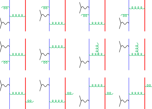
Refer to caption
Figure 15: Feynman graphs appearing in the calculation of the real radiation amplitudes.

Infrared singularities are handled using the subtraction method Ellis:1980wv implemented using the dipole formulation Catani:1996vz and extended to the case of massive emitters and spectators Catani:2002hc . The full calculation will be made available as part of the the MCFM code MCFM ; Campbell:1999ah .

To provide a point of comparison we have timed the evaluation of the complete one-loop contribution, i.e. the interference in Eq. (25), summed over all four possible spin labels on the heavy quark line. Using a standard 2.662.662.66 GHz machine and compiling the code with the -O2 flag of gfortran this operation takes 444ms for a single phase space point, which is about a factor of sixty slower than evaluating the corresponding massless amplitudes as implemented in MCFM.

VIII.1 Checks on the calculation

A number of checks have been performed at various stages of the calculation.

  1. 1.

    At the level of the one-loop amplitude, we have cross-checked our calculation with a numerical implementation of generalized d𝑑d-dimensional unitarity Ellis:2008qc . This check confirms the coefficients of all the scalar integrals and rational terms, as well as the complete (unrenormalized) amplitude, at any given phase space point. The values of the unrenormalized one-loop amplitudes at a specific phase space point are given in Appendix E. These numbers may be useful in performing a check of our calculation.

  2. 2.

    The cancellation of infrared singularities is performed using a slight extension of the original dipole formulation in which the extent of each subtraction region is controlled by an additional parameter Nagy:1998bb ; Nagy:2003tz . This parameter also appears in the integrated form of the dipole counterterms in such a way that the sum of real and virtual radiation does not depend upon its value. We have checked that this independence is indeed manifest in our calculation.

  3. 3.

    We have checked that our final results for the Wbb¯𝑊𝑏¯𝑏Wb\bar{b} integrated cross section agree with the values reported in the earlier calculations of Refs. Febres Cordero:2006sj ; Cordero:2009kv ; Cordero:2010qn .

VIII.2 Phenomenology

mW=80.44subscript𝑚𝑊80.44m_{W}=80.44 GeV mb=4.62subscript𝑚𝑏4.62m_{b}=4.62 GeV
mt=172.6subscript𝑚𝑡172.6m_{t}=172.6 GeV sin2θw=0.223superscript2subscript𝜃𝑤0.223\sin^{2}\theta_{w}=0.223
GF=1.16639105GeV2subscript𝐺𝐹1.16639superscript105superscriptGeV2G_{F}=1.16639\cdot 10^{-5}~{}\mbox{GeV}^{-2} α=2πGFmW2sin2θw𝛼2𝜋subscript𝐺𝐹superscriptsubscript𝑚𝑊2superscript2subscript𝜃𝑤\alpha=\frac{\sqrt{2}}{\pi}G_{F}m_{W}^{2}\sin^{2}\theta_{w}
Vud=Vcs=0.974subscript𝑉𝑢𝑑subscript𝑉𝑐𝑠0.974V_{ud}=V_{cs}=0.974 GeV Vus=Vcd=0.227subscript𝑉𝑢𝑠subscript𝑉𝑐𝑑0.227V_{us}=V_{cd}=0.227
PDF set: CTEQ6L1
αs(mW+2mb)=0.130345subscript𝛼𝑠subscript𝑚𝑊2subscript𝑚𝑏0.130345\alpha_{s}(m_{W}+2m_{b})=0.130345
}}\Biggr{\}} LO
PDF set: CTEQ6M
αs(mW+2mb)=0.118298subscript𝛼𝑠subscript𝑚𝑊2subscript𝑚𝑏0.118298\alpha_{s}(m_{W}+2m_{b})=0.118298
}}\Biggr{\}} NLO
Table 4: Inputs used for the results presented in section VIII.

For now we present only a limited set of results, focussing mainly on the comparison with previous calculations and presenting a simple distribution involving the decay products of the W𝑊W boson. We leave a detailed phenomenological study for a future work.

For convenience, we choose the same set of input parameters here as reported in Ref. Cordero:2009kv , which are summarized in Table 4. The final state is defined by the following cuts on the b𝑏b-jets,

pTb>25GeV,|ηb|<2.5,formulae-sequencesuperscriptsubscript𝑝𝑇𝑏25GeVsuperscript𝜂𝑏2.5p_{T}^{b}>25~{}\mbox{GeV}\;,\qquad|\eta^{b}|<2.5\;, (111)

where the jets are identified using the kTsubscript𝑘𝑇k_{T} clustering algorithm with pseudo-cone size R=0.7𝑅0.7R=0.7. The results presented here are inclusive of the additional jet that may be present at NLO.

As already discussed previously, although we treat the b𝑏b-quark as a massive particle when it appears in the final state, we use nlf=5subscript𝑛lf5n_{{\rm lf}}=5 light flavours in the running of αssubscript𝛼𝑠\alpha_{s} and the PDF evolution. This is primarily for comparison with previous work Cordero:2009kv . We note that because of the smallness of Vcbsubscript𝑉𝑐𝑏V_{cb} and Vubsubscript𝑉𝑢𝑏V_{ub} the b𝑏b-quark distributions in the initial state make a negligible contribution. However because s23>4mb2subscript𝑠234superscriptsubscript𝑚𝑏2s_{23}>4m_{b}^{2} it is more appropriate to have a strong coupling constant running with nlf=5subscript𝑛lf5n_{{\rm lf}}=5 active flavours.

We first present the cross sections for this process at the LHC, for center-of-mass energies s=7𝑠7\sqrt{s}=7, 888 and 141414 TeV. The results at LO and NLO are shown in Table 5 where we have used a scale choice μR=μF=mW+2mbsubscript𝜇𝑅subscript𝜇𝐹subscript𝑚𝑊2subscript𝑚𝑏\mu_{R}=\mu_{F}=m_{W}+2m_{b} throughout, again to facilitate comparison with Ref. Cordero:2009kv . For these results no cuts are applied on the decay products of the W𝑊W boson and the corresponding branching ratio is removed, so that the reported cross sections are for a W𝑊W that does not decay. In this way, one sees from the final column (s=14𝑠14\sqrt{s}=14 TeV) that our results agree with those reported in Ref. Cordero:2009kv at the level of 0.50.50.5%. As noted in earlier work Campbell:2003hd , at LHC energies the NLO corrections are substantial because of the influence of the quark-gluon initial state.

s𝑠\sqrt{s}    777 TeV    888 TeV    141414 TeV
W+bb¯superscript𝑊𝑏¯𝑏W^{+}b\bar{b} LO 4.456(2) 5.157(2) 9.041(3)
NLO 8.655(9) 10.58(2) 23.51(3)
Wbb¯superscript𝑊𝑏¯𝑏W^{-}b\bar{b} LO 2.588(2) 3.109(1) 6.256(2)
NLO 5.053(5) 6.353(6) 15.55(2)
Table 5: LO and NLO cross sections (in picobarns) for Wbb¯𝑊𝑏¯𝑏Wb\bar{b} production at various energies of the LHC. Integration errors are shown in parentheses.

To illustrate a new quantity that may now be computed at NLO accuracy, in Fig. 16 we show the LO and NLO predictions for the quantity Rljminsuperscriptsubscript𝑅𝑙𝑗minR_{lj}^{\rm{min}} which is defined as the separation between the charged lepton and the closest jet,

Rljmin=min{jets}(ηleptonηjet)2+(ϕleptonϕjet)2.superscriptsubscript𝑅𝑙𝑗minsubscriptjetssuperscriptsubscript𝜂leptonsubscript𝜂jet2superscriptsubscriptitalic-ϕleptonsubscriptitalic-ϕjet2R_{lj}^{\rm{min}}=\min_{\{\rm{jets}\}}\sqrt{(\eta_{\rm{lepton}}-\eta_{\rm{jet}})^{2}+(\phi_{\rm{lepton}}-\phi_{\rm{jet}})^{2}}\;. (112)

In this equation the azimuthal angles and pseudorapidities (in the lab-frame) of the lepton and jets are denoted by ϕitalic-ϕ\phi and η𝜂\eta respectively.

Refer to caption
Figure 16: Distribution of the minimum separation between the electron and any jet, Rljsubscript𝑅𝑙𝑗R_{lj}, defined in Eq. (112) of the text, for Wbb¯superscript𝑊𝑏¯𝑏W^{-}b{\bar{b}} production at the 141414 TeV LHC. The distributions are normalized to unit area.

We see that the effect of the NLO corrections on the shape of this distribution is relatively minor, visible only for Rjlmin>1.5superscriptsubscript𝑅𝑗𝑙min1.5R_{jl}^{\rm min}>1.5.

IX Conclusions

We have presented the first computation of the Wbb¯𝑊𝑏¯𝑏Wb\bar{b} cross section with massive b𝑏b-quarks, including the lepton correlations present in the decay of the W𝑊W-boson. This calculation required knowledge of the one-loop virtual corrections to the qQ¯Qq¯¯𝑞¯𝑄𝑄¯𝑞¯q{\bar{Q}}{\vphantom{{\bar{Q}}}{Q}}{\bar{q}}{\overline{\ell}}\ell process retaining the mass for the heavy quarks Q𝑄Q. The one-loop amplitude was obtained using the spinor helicity formalism. This method has been extensively used for one-loop calculations with massless quarks, but rarely with massive quarks. The calculation required a number of modifications of standard techniques to cope with the presence of the mass.

Although our results are analytic we have not yet simplified them sufficiently to publish them in a journal article. Our results for the one-loop amplitudes will be included in the released version of MCFM, which is an appropriate method of publishing such results. Our analytic results did lead to a code which is fast and numerically stable. Using this code we intend to study the detailed phenomenology of this process in a future publication.

Acknowledgements

We are happy to acknowledge useful discussions with Fabrizio Caola and Kirill Melnikov. The work of SB has been supported in part by Danish Natural Science Research Council grant 10-084954. Fermilab is operated by Fermi Research Alliance, LLC, under contract DE-AC02-07CH11359 with the United States Department of Energy.

Appendix A Notation for spinor products

The spinor notation is almost standard, but because of the presence of massive particles, it is important to make it explicit. We adopt the following notation for massless spinors,

|iket𝑖\displaystyle|i\rangle =|i+=u+(ki),|i]\displaystyle=|i+\rangle=u_{+}(k_{i}),\;|i] =|i=u(ki),absentketlimit-from𝑖subscript𝑢subscript𝑘𝑖\displaystyle=|i-\rangle=u_{-}(k_{i})\;,
i|bra𝑖\displaystyle\langle i| =i|=u¯(ki),[i|\displaystyle=\langle i-|=\bar{u}_{-}(k_{i}),\;[i| =i+|=u¯+(ki).absentbralimit-from𝑖subscript¯𝑢subscript𝑘𝑖\displaystyle=\langle i+|=\bar{u}_{+}(k_{i})\;. (113)

Further the spinor products are defined as,

ijdelimited-⟨⟩𝑖𝑗\displaystyle\left\langle i\,j\right\rangle =\displaystyle= i|j+=u¯(ki)u+(kj),inner-productlimit-from𝑖limit-from𝑗subscript¯𝑢subscript𝑘𝑖subscript𝑢subscript𝑘𝑗\displaystyle\langle i-|j+\rangle=\bar{u}_{-}(k_{i})u_{+}(k_{j})\;,
[ij]delimited-[]𝑖𝑗\displaystyle\left[i\,j\right] =\displaystyle= i+|j=u¯+(ki)u(kj),inner-productlimit-from𝑖limit-from𝑗subscript¯𝑢subscript𝑘𝑖subscript𝑢subscript𝑘𝑗\displaystyle\langle i+|j-\rangle=\bar{u}_{+}(k_{i})u_{-}(k_{j})\;, (114)

with ki,kjsubscript𝑘𝑖subscript𝑘𝑗k_{i},k_{j} massless particles. With our convention,

ij[ji]=2kikj=sij.delimited-⟨⟩𝑖𝑗delimited-[]𝑗𝑖2subscript𝑘𝑖subscript𝑘𝑗subscript𝑠𝑖𝑗\left\langle i\,j\right\rangle\;\left[j\,i\right]=2k_{i}\cdot k_{j}=s_{ij}\;. (115)

We also define the spinor strings.

i|j|k]delimited-⟨]𝑖𝑗𝑘\displaystyle\langle i|j|k] \displaystyle\equiv ki|kj|kk,quantum-operator-productlimit-fromsubscript𝑘𝑖subscript𝑘𝑗limit-fromsubscript𝑘𝑘\displaystyle\langle k_{i}-|\hbox to0.0pt{$\;\!\!\not$\hss}{k}_{j}|k_{k}-\rangle\;,
i|j+k|l]delimited-⟨]𝑖𝑗𝑘𝑙\displaystyle\langle i|j+k|l] \displaystyle\equiv ki|(kj+kk)|kl,quantum-operator-productlimit-fromsubscript𝑘𝑖subscript𝑘𝑗subscript𝑘𝑘limit-fromsubscript𝑘𝑙\displaystyle\langle k_{i}-|(\hbox to0.0pt{$\;\!\!\not$\hss}{k}_{j}+\hbox to0.0pt{$\;\!\!\not$\hss}{k}_{k})|k_{l}-\rangle\;,
i|jk|lquantum-operator-product𝑖𝑗𝑘𝑙\displaystyle\langle\mskip-1.0mu{i}|jk|{l}\mskip-1.0mu\rangle \displaystyle\equiv ki|kjkk|kl+.quantum-operator-productlimit-fromsubscript𝑘𝑖subscript𝑘𝑗subscript𝑘𝑘limit-fromsubscript𝑘𝑙\displaystyle\langle k_{i}-|\hbox to0.0pt{$\;\!\!\not$\hss}{k}_{j}\hbox to0.0pt{$\;\!\!\not$\hss}{k}_{k}|k_{l}+\rangle\;. (116)

For the case of a massless momentum kjsubscript𝑘𝑗k_{j} we may write,

i|j|k]=ij[jk],\langle i|j|k]=\left\langle i\,j\right\rangle\left[j\,k\right]\;, (117)

but for the case of a massive momentum, (in our notation the momenta p2subscript𝑝2p_{2} and p3subscript𝑝3p_{3}), this separation in no longer possible. As a compact notation we therefore write in this case i|𝐣|k]delimited-⟨]𝑖𝐣𝑘\langle i|\hbox to0.0pt{$\;\!\!\not$\hss}{{\bf j}}|k], denoting the massive momentum by a bold-face symbol.

The Schouten identity,

[ik][mn]=[in][mk]+[im][kn],delimited-[]𝑖𝑘delimited-[]𝑚𝑛delimited-[]𝑖𝑛delimited-[]𝑚𝑘delimited-[]𝑖𝑚delimited-[]𝑘𝑛[i\,k][m\,n]=[i\,n][m\,k]+[i\,m][k\,n]\;, (118)

may be applied to these compound quantities. Thus we have,

i|𝐣|k][mn]=i|𝐣|n][mk]+i|𝐣|m][kn].\langle i|\hbox to0.0pt{$\;\!\!\not$\hss}{{\bf j}}|k][m\,n]=\langle i|\hbox to0.0pt{$\;\!\!\not$\hss}{{\bf j}}|n][m\,k]+\langle i|\hbox to0.0pt{$\;\!\!\not$\hss}{{\bf j}}|m][k\,n]\;. (119)

Appendix B Tree level results

B.1 Results for A(1g,2Q¯,3Q,4g)𝐴subscript1𝑔subscript2¯𝑄subscript3𝑄subscript4𝑔A(1_{g},2_{\bar{Q}},3_{Q},4_{g})

As an example of the use of the massive spinors employed in the calculation we consider the tree-level two-quark two-gluon amplitude, A(1g,2Q¯,3Q,4g)𝐴subscript1𝑔subscript2¯𝑄subscript3𝑄subscript4𝑔A(1_{g},2_{\bar{Q}},3_{Q},4_{g}). The fermions, with momenta p2subscript𝑝2p_{2} and p3subscript𝑝3p_{3} have a common mass m𝑚m. The momenta are all outgoing so that k1+p2+p3+k4=0subscript𝑘1subscript𝑝2subscript𝑝3subscript𝑘40k_{1}+p_{2}+p_{3}+k_{4}=0.

Refer to caption
Figure 17: Diagrams for two gluons coupling to a massive quark line.

The amplitude is obtained by summing the contributions of the three Feynman diagrams, M(a)superscript𝑀𝑎M^{(a)}, M(b)superscript𝑀𝑏M^{(b)} and M(c)superscript𝑀𝑐M^{(c)} shown in Fig. 17,

A4tree=i2g2[(TC4TC1)i3i2(M(a)+M(b))+(TC1TC4)i3i2(M(c)M(b))],superscriptsubscript𝐴4tree𝑖2superscript𝑔2delimited-[]subscriptsuperscript𝑇subscript𝐶4superscript𝑇subscript𝐶1subscript𝑖3subscript𝑖2superscript𝑀𝑎superscript𝑀𝑏subscriptsuperscript𝑇subscript𝐶1superscript𝑇subscript𝐶4subscript𝑖3subscript𝑖2superscript𝑀𝑐superscript𝑀𝑏\displaystyle A_{4}^{\rm tree}=-\frac{i}{2}g^{2}\Bigg{[}(T^{C_{4}}T^{C_{1}})_{i_{3}i_{2}}(M^{(a)}+M^{(b)})+(T^{C_{1}}T^{C_{4}})_{i_{3}i_{2}}(M^{(c)}-M^{(b)})\Bigg{]}\;, (120)

Normalizing the colour matrices as follows,

TrTATB=δAB,Trsuperscript𝑇𝐴superscript𝑇𝐵superscript𝛿𝐴𝐵{\rm Tr}~{}T^{A}T^{B}=\delta^{AB}\;, (121)

an explicit calculation yields the following contributions,

M(a)superscript𝑀𝑎\displaystyle M^{(a)} =\displaystyle= u¯(p3)ϵ4p34+mp342m2ϵ1v(p2),¯𝑢subscript𝑝3subscriptitalic-ϵ4subscript𝑝34𝑚superscriptsubscript𝑝342superscript𝑚2subscriptitalic-ϵ1𝑣subscript𝑝2\displaystyle\bar{u}(p_{3})\hbox to0.0pt{$\;\!\!\not$\hss}{\epsilon}_{4}\frac{\hbox to0.0pt{$\;\!\!\not$\hss}{p_{34}}+m}{p_{34}^{2}-m^{2}}\hbox to0.0pt{$\;\!\!\not$\hss}{\epsilon}_{1}v(p_{2})\;, (122)
M(b)superscript𝑀𝑏\displaystyle M^{(b)} =\displaystyle= ϵ1ϵ4k1k4u¯(p3)k1v(p2)k1ϵ4k1k4u¯(p3)ϵ1v(p2)+k4ϵ1k1k4u¯(p3)ϵ4v(p2),subscriptitalic-ϵ1subscriptitalic-ϵ4subscript𝑘1subscript𝑘4¯𝑢subscript𝑝3subscript𝑘1𝑣subscript𝑝2subscript𝑘1subscriptitalic-ϵ4subscript𝑘1subscript𝑘4¯𝑢subscript𝑝3subscriptitalic-ϵ1𝑣subscript𝑝2subscript𝑘4subscriptitalic-ϵ1subscript𝑘1subscript𝑘4¯𝑢subscript𝑝3subscriptitalic-ϵ4𝑣subscript𝑝2\displaystyle\frac{\epsilon_{1}\cdot\epsilon_{4}}{k_{1}\cdot k_{4}}\bar{u}(p_{3})\hbox to0.0pt{$\;\!\!\not$\hss}{k}_{1}v(p_{2})-\frac{k_{1}\cdot\epsilon_{4}}{k_{1}\cdot k_{4}}\bar{u}(p_{3})\hbox to0.0pt{$\;\!\!\not$\hss}{\epsilon}_{1}v(p_{2})+\frac{k_{4}\cdot\epsilon_{1}}{k_{1}\cdot k_{4}}\bar{u}(p_{3})\hbox to0.0pt{$\;\!\!\not$\hss}{\epsilon}_{4}v(p_{2})\;, (123)
M(c)superscript𝑀𝑐\displaystyle M^{(c)} =\displaystyle= u¯(p3)ϵ1p13+mp132m2ϵ4v(p2),¯𝑢subscript𝑝3subscriptitalic-ϵ1subscript𝑝13𝑚superscriptsubscript𝑝132superscript𝑚2subscriptitalic-ϵ4𝑣subscript𝑝2\displaystyle\bar{u}(p_{3})\hbox to0.0pt{$\;\!\!\not$\hss}{\epsilon}_{1}\frac{\hbox to0.0pt{$\;\!\!\not$\hss}{p_{13}}+m}{p_{13}^{2}-m^{2}}\hbox to0.0pt{$\;\!\!\not$\hss}{\epsilon}_{4}v(p_{2})\;, (124)

where p13=k1+p3subscript𝑝13subscript𝑘1subscript𝑝3p_{13}=k_{1}+p_{3} and p34=p3+k4subscript𝑝34subscript𝑝3subscript𝑘4p_{34}=p_{3}+k_{4}. From Eq. (10) we write the massive spinors as,

u¯(p3)¯𝑢subscript𝑝3\displaystyle\bar{u}(p_{3}) =\displaystyle= N3u¯(k2)(p3+m),subscript𝑁3¯𝑢subscript𝑘2subscript𝑝3𝑚\displaystyle N_{3}\bar{u}(k_{2})(\hbox to0.0pt{$\;\!\!\not$\hss}{p}_{3}+m)\;, (125)
v(p2)𝑣subscript𝑝2\displaystyle v(p_{2}) =\displaystyle= N2(p2m)v(k3),subscript𝑁2subscript𝑝2𝑚𝑣subscript𝑘3\displaystyle N_{2}(\hbox to0.0pt{$\;\!\!\not$\hss}{p}_{2}-m)v(k_{3})\;, (126)

and then reorganize the calculation by using the identities Morgan:1995te ,

(p3+m)ϵ4subscript𝑝3𝑚subscriptitalic-ϵ4\displaystyle(\hbox to0.0pt{$\;\!\!\not$\hss}{p}_{3}+m)\hbox to0.0pt{$\;\!\!\not$\hss}{\epsilon}_{4} \displaystyle\equiv (p34k4+m)ϵ4subscript𝑝34subscript𝑘4𝑚subscriptitalic-ϵ4\displaystyle(\hbox to0.0pt{$\;\!\!\not$\hss}{p}_{34}-\hbox to0.0pt{$\;\!\!\not$\hss}{k}_{4}+m)\hbox to0.0pt{$\;\!\!\not$\hss}{\epsilon}_{4} (127)
\displaystyle\equiv (2p34k4)ϵ412[k4,ϵ4]ϵ4(p34m),2subscript𝑝34subscript𝑘4subscriptitalic-ϵ412subscript𝑘4subscriptitalic-ϵ4subscriptitalic-ϵ4subscript𝑝34𝑚\displaystyle(2p_{34}-k_{4})\cdot\epsilon_{4}-\frac{1}{2}[\hbox to0.0pt{$\;\!\!\not$\hss}{k}_{4},\hbox to0.0pt{$\;\!\!\not$\hss}{\epsilon}_{4}]-\hbox to0.0pt{$\;\!\!\not$\hss}{\epsilon}_{4}(\hbox to0.0pt{$\;\!\!\not$\hss}{p}_{34}-m)\;,
(p12+m)ϵ1subscript𝑝12𝑚subscriptitalic-ϵ1\displaystyle(-\hbox to0.0pt{$\;\!\!\not$\hss}{p}_{12}+m)\hbox to0.0pt{$\;\!\!\not$\hss}{\epsilon}_{1} \displaystyle\equiv (2p2+k1)ϵ112[k1,ϵ1]+ϵ1(p2+m).2subscript𝑝2subscript𝑘1subscriptitalic-ϵ112subscript𝑘1subscriptitalic-ϵ1subscriptitalic-ϵ1subscript𝑝2𝑚\displaystyle-(2p_{2}+k_{1})\cdot\epsilon_{1}-\frac{1}{2}[\hbox to0.0pt{$\;\!\!\not$\hss}{k}_{1},\hbox to0.0pt{$\;\!\!\not$\hss}{\epsilon}_{1}]+\hbox to0.0pt{$\;\!\!\not$\hss}{\epsilon}_{1}(\hbox to0.0pt{$\;\!\!\not$\hss}{p}_{2}+m)\;. (128)

Inserting these identities we may write new forms for M(a)superscript𝑀𝑎M^{(a)} and M(c)superscript𝑀𝑐M^{(c)},

M(i)superscript𝑀𝑖\displaystyle M^{(i)} =\displaystyle= N2N3u¯(k2)Γ(i)(p2m)v(k3),i=(a,b,c)subscript𝑁2subscript𝑁3¯𝑢subscript𝑘2superscriptΓ𝑖subscript𝑝2𝑚𝑣subscript𝑘3𝑖𝑎𝑏𝑐\displaystyle N_{2}N_{3}\bar{u}(k_{2})\;\Gamma^{(i)}\;(\hbox to0.0pt{$\;\!\!\not$\hss}{p}_{2}-m)\;v(k_{3})\;,\;\;\;i=(a,b,c) (129)
Γ(a)superscriptΓ𝑎\displaystyle\Gamma^{(a)} =\displaystyle= {[2p3ϵ412[k4,ϵ4]]12p3k4[2p2ϵ112[k1,ϵ1]]ϵ4ϵ1},delimited-[]2subscript𝑝3subscriptitalic-ϵ412subscript𝑘4subscriptitalic-ϵ412subscript𝑝3subscript𝑘4delimited-[]2subscript𝑝2subscriptitalic-ϵ112subscript𝑘1subscriptitalic-ϵ1subscriptitalic-ϵ4subscriptitalic-ϵ1\displaystyle\Big{\{}\Big{[}2p_{3}\cdot\epsilon_{4}-\frac{1}{2}[\hbox to0.0pt{$\;\!\!\not$\hss}{k}_{4},\hbox to0.0pt{$\;\!\!\not$\hss}{\epsilon}_{4}]\Big{]}\frac{1}{2p_{3}\cdot k_{4}}\Big{[}-2p_{2}\cdot\epsilon_{1}-\frac{1}{2}[\hbox to0.0pt{$\;\!\!\not$\hss}{k}_{1},\hbox to0.0pt{$\;\!\!\not$\hss}{\epsilon}_{1}]\Big{]}-\hbox to0.0pt{$\;\!\!\not$\hss}{\epsilon}_{4}\hbox to0.0pt{$\;\!\!\not$\hss}{\epsilon}_{1}\Big{\}}\;, (130)
Γ(c)superscriptΓ𝑐\displaystyle\Gamma^{(c)} =\displaystyle= {[2p3ϵ112[k1,ϵ1]]12p3k1[2p2ϵ412[k4,ϵ4]]ϵ1ϵ4}.delimited-[]2subscript𝑝3subscriptitalic-ϵ112subscript𝑘1subscriptitalic-ϵ112subscript𝑝3subscript𝑘1delimited-[]2subscript𝑝2subscriptitalic-ϵ412subscript𝑘4subscriptitalic-ϵ4subscriptitalic-ϵ1subscriptitalic-ϵ4\displaystyle\Big{\{}\Big{[}2p_{3}\cdot\epsilon_{1}-\frac{1}{2}[\hbox to0.0pt{$\;\!\!\not$\hss}{k}_{1},\hbox to0.0pt{$\;\!\!\not$\hss}{\epsilon}_{1}]\Big{]}\frac{1}{2p_{3}\cdot k_{1}}\Big{[}-2p_{2}\cdot\epsilon_{4}-\frac{1}{2}[\hbox to0.0pt{$\;\!\!\not$\hss}{k}_{4},\hbox to0.0pt{$\;\!\!\not$\hss}{\epsilon}_{4}]\Big{]}-\hbox to0.0pt{$\;\!\!\not$\hss}{\epsilon}_{1}\hbox to0.0pt{$\;\!\!\not$\hss}{\epsilon}_{4}\Big{\}}\;. (131)

These formulae have the advantage that the m𝑚m dependence is corralled in a single place, in Eq. (129). Moreover the overall form is simple and the last term in Eqs. (130, 131) does not contain the massive propagator. Γ(b)superscriptΓ𝑏\Gamma^{(b)} can be read off from Eq. (123). Inserting the appropriate polarization vectors we find,

iA(1g,2Q¯+,3Q,4g+)𝑖𝐴superscriptsubscript1𝑔superscriptsubscript2¯𝑄superscriptsubscript3𝑄superscriptsubscript4𝑔\displaystyle-iA(1_{g}^{-},2_{\bar{Q}}^{+},3_{\vphantom{{\bar{Q}}}{Q}}^{-},4_{g}^{+}) =\displaystyle= [2 4]21|𝟐|4][1 4][2 3]4|𝟑|4],\displaystyle-\frac{\left[2\,4\right]^{2}\langle\mskip-1.0mu{1}|\hbox to0.0pt{$\;\!\!\not$\hss}{\bf 2}|{4}\mskip-1.0mu]}{\left[1\,4\right]\left[2\,3\right]\langle\mskip-1.0mu{4}|\hbox to0.0pt{$\;\!\!\not$\hss}{\bf 3}|{4}\mskip-1.0mu]}\;,
iA(1g,2Q¯,3Q+,4g+)𝑖𝐴superscriptsubscript1𝑔superscriptsubscript2¯𝑄superscriptsubscript3𝑄superscriptsubscript4𝑔\displaystyle-iA(1_{g}^{-},2_{\bar{Q}}^{-},3_{\vphantom{{\bar{Q}}}{Q}}^{+},4_{g}^{+}) =\displaystyle= 1 221|𝟑|4]1 42 34|𝟑|4],\displaystyle-\frac{{\left\langle 1\,2\right\rangle}^{2}\langle\mskip-1.0mu{1}|\hbox to0.0pt{$\;\!\!\not$\hss}{\bf 3}|{4}\mskip-1.0mu]}{\left\langle 1\,4\right\rangle\left\langle 2\,3\right\rangle\langle\mskip-1.0mu{4}|\hbox to0.0pt{$\;\!\!\not$\hss}{\bf 3}|{4}\mskip-1.0mu]}\;,
iA(1g,2Q¯,3Q,4g+)𝑖𝐴superscriptsubscript1𝑔superscriptsubscript2¯𝑄superscriptsubscript3𝑄superscriptsubscript4𝑔\displaystyle-iA(1_{g}^{-},2_{\bar{Q}}^{-},3_{\vphantom{{\bar{Q}}}{Q}}^{-},4_{g}^{+}) =\displaystyle= 2(β+β)m[2 3]1 32[3 4]21 4[1 4]4|𝟑|4],\displaystyle 2(\beta_{+}-\beta_{-})\frac{m}{\left[2\,3\right]}\frac{{\left\langle 1\,3\right\rangle}^{2}{\left[3\,4\right]}^{2}}{\left\langle 1\,4\right\rangle\left[1\,4\right]\langle\mskip-1.0mu{4}|\hbox to0.0pt{$\;\!\!\not$\hss}{\bf 3}|{4}\mskip-1.0mu]}\;,
iA(1g,2Q¯+,3Q+,4g+)𝑖𝐴superscriptsubscript1𝑔superscriptsubscript2¯𝑄superscriptsubscript3𝑄superscriptsubscript4𝑔\displaystyle-iA(1_{g}^{-},2_{\bar{Q}}^{+},3_{\vphantom{{\bar{Q}}}{Q}}^{+},4_{g}^{+}) =\displaystyle= 2(β+β)m2 31 32[3 4]21 4[1 4]4|𝟑|4],\displaystyle 2(\beta_{+}-\beta_{-})\frac{m}{\left\langle 2\,3\right\rangle}\frac{{\left\langle 1\,3\right\rangle}^{2}{\left[3\,4\right]}^{2}}{\left\langle 1\,4\right\rangle\left[1\,4\right]\langle\mskip-1.0mu{4}|\hbox to0.0pt{$\;\!\!\not$\hss}{\bf 3}|{4}\mskip-1.0mu]}\;,
iA(1g,2Q¯+,3Q,4g)𝑖𝐴superscriptsubscript1𝑔superscriptsubscript2¯𝑄superscriptsubscript3𝑄superscriptsubscript4𝑔\displaystyle-iA(1_{g}^{-},2_{\bar{Q}}^{+},3_{\vphantom{{\bar{Q}}}{Q}}^{-},4_{g}^{-}) =\displaystyle= 0,0\displaystyle 0\;,
iA(1g,2Q¯,3Q+,4g)𝑖𝐴superscriptsubscript1𝑔superscriptsubscript2¯𝑄superscriptsubscript3𝑄superscriptsubscript4𝑔\displaystyle-iA(1_{g}^{-},2_{\bar{Q}}^{-},3_{\vphantom{{\bar{Q}}}{Q}}^{+},4_{g}^{-}) =\displaystyle= 0,0\displaystyle 0\;,
iA(1g,2Q¯+,3Q+,4g)𝑖𝐴superscriptsubscript1𝑔superscriptsubscript2¯𝑄superscriptsubscript3𝑄superscriptsubscript4𝑔\displaystyle-iA(1_{g}^{-},2_{\bar{Q}}^{+},3_{\vphantom{{\bar{Q}}}{Q}}^{+},4_{g}^{-}) =\displaystyle= mβ+2 31 424|𝟑|4],𝑚subscript𝛽delimited-⟨⟩23superscriptdelimited-⟨⟩142delimited-⟨]434\displaystyle-\frac{m\beta_{+}}{\left\langle 2\,3\right\rangle}\frac{{\left\langle 1\,4\right\rangle}^{2}}{\langle\mskip-1.0mu{4}|\hbox to0.0pt{$\;\!\!\not$\hss}{\bf 3}|{4}\mskip-1.0mu]}\;,
iA(1g,2Q¯,3Q,4g)𝑖𝐴superscriptsubscript1𝑔superscriptsubscript2¯𝑄superscriptsubscript3𝑄superscriptsubscript4𝑔\displaystyle-iA(1_{g}^{-},2_{\bar{Q}}^{-},3_{\vphantom{{\bar{Q}}}{Q}}^{-},4_{g}^{-}) =\displaystyle= mβ[2 3]1 424|𝟑|4].𝑚subscript𝛽delimited-[]23superscriptdelimited-⟨⟩142delimited-⟨]434\displaystyle\frac{m\beta_{-}}{\left[2\,3\right]}\frac{{\left\langle 1\,4\right\rangle}^{2}}{\langle\mskip-1.0mu{4}|\hbox to0.0pt{$\;\!\!\not$\hss}{\bf 3}|{4}\mskip-1.0mu]}\;. (132)

B.2 Results for A(1q,2q¯,3g)𝐴subscript1𝑞subscript2¯𝑞subscript3𝑔A(1_{q},2_{\bar{q}},3_{g})

The tree-level results for the simple qq¯g𝑞¯𝑞𝑔q\bar{q}g amplitudes, stripped of overall colour and coupling constant factors, are well known:

iA(1q,2q¯+,3g)𝑖𝐴superscriptsubscript1𝑞superscriptsubscript2¯𝑞superscriptsubscript3𝑔\displaystyle-iA(1_{\vphantom{{\bar{q}}}{q}}^{-},2_{\bar{q}}^{+},3_{g}^{-}) =\displaystyle= 1 321 2,superscriptdelimited-⟨⟩132delimited-⟨⟩12\displaystyle-\frac{{\left\langle 1\,3\right\rangle}^{2}}{\left\langle 1\,2\right\rangle}\;, (133)
iA(1q,2q¯+,3g+)𝑖𝐴superscriptsubscript1𝑞superscriptsubscript2¯𝑞superscriptsubscript3𝑔\displaystyle-iA(1_{\vphantom{{\bar{q}}}{q}}^{-},2_{\bar{q}}^{+},3_{g}^{+}) =\displaystyle= [2 3]2[1 2].superscriptdelimited-[]232delimited-[]12\displaystyle-\frac{{\left[2\,3\right]}^{2}}{\left[1\,2\right]}\;. (134)

B.3 Results for A(1q,2q¯,3g,4l¯,5l)𝐴subscript1𝑞subscript2¯𝑞subscript3𝑔subscript4¯𝑙subscript5𝑙A(1_{q},2_{\bar{q}},3_{g},4_{{\bar{l}}},5_{l})

The tree-level amplitudes for qq¯Wg𝑞¯𝑞𝑊𝑔q\bar{q}Wg are also rather simple. Removing the colour and coupling constants as normal we have,

iA(1q,2q¯+,3g,4l¯+,5l)𝑖𝐴superscriptsubscript1𝑞superscriptsubscript2¯𝑞superscriptsubscript3𝑔superscriptsubscript4¯𝑙superscriptsubscript5𝑙\displaystyle-iA(1_{\vphantom{{\bar{q}}}{q}}^{-},2_{\bar{q}}^{+},3_{g}^{-},4_{\bar{l}}^{+},5_{\vphantom{{\bar{l}}}{l}}^{-}) =\displaystyle= [2 4]2[1 3][2 3][4 5],superscriptdelimited-[]242delimited-[]13delimited-[]23delimited-[]45\displaystyle-\frac{\left[2\,4\right]^{2}}{\left[1\,3\right]\left[2\,3\right]\left[4\,5\right]}\;,
iA(1q,2q¯+,3g+,5l¯+,4l)𝑖𝐴superscriptsubscript1𝑞superscriptsubscript2¯𝑞superscriptsubscript3𝑔superscriptsubscript5¯𝑙superscriptsubscript4𝑙\displaystyle-iA(1_{\vphantom{{\bar{q}}}{q}}^{-},2_{\bar{q}}^{+},3_{g}^{+},5_{\bar{l}}^{+},4_{\vphantom{{\bar{l}}}{l}}^{-}) =\displaystyle= 1 521 32 34 5.superscriptdelimited-⟨⟩152delimited-⟨⟩13delimited-⟨⟩23delimited-⟨⟩45\displaystyle\frac{\left\langle 1\,5\right\rangle^{2}}{\left\langle 1\,3\right\rangle\left\langle 2\,3\right\rangle\left\langle 4\,5\right\rangle}\;. (135)

Appendix C Scalar integrals

We work in the Bjorken-Drell metric so that l2=l02l12l22l32superscript𝑙2superscriptsubscript𝑙02superscriptsubscript𝑙12superscriptsubscript𝑙22superscriptsubscript𝑙32l^{2}=l_{0}^{2}-l_{1}^{2}-l_{2}^{2}-l_{3}^{2}. The definition of the integrals is as follows,

A0(m12)=μ4DiπD2rΓdDl1(l2m12),subscript𝐴0superscriptsubscript𝑚12superscript𝜇4𝐷𝑖superscript𝜋𝐷2subscript𝑟Γsuperscript𝑑𝐷𝑙1superscript𝑙2superscriptsubscript𝑚12\displaystyle A_{0}(m_{1}^{2})=\frac{\mu^{4-D}}{i\pi^{\frac{D}{2}}r_{\Gamma}}\int d^{D}l\;\frac{1}{(l^{2}-m_{1}^{2})}\,,
B0(p1;m1,m2)=μ4DiπD2rΓdDl1(l2m12)((l+p1)2m22),subscript𝐵0subscript𝑝1subscript𝑚1subscript𝑚2superscript𝜇4𝐷𝑖superscript𝜋𝐷2subscript𝑟Γsuperscript𝑑𝐷𝑙1superscript𝑙2superscriptsubscript𝑚12superscript𝑙subscript𝑝12superscriptsubscript𝑚22\displaystyle B_{0}(p_{1};m_{1},m_{2})=\frac{\mu^{4-D}}{i\pi^{\frac{D}{2}}r_{\Gamma}}\int d^{D}l\;\frac{1}{(l^{2}-m_{1}^{2})((l+p_{1})^{2}-m_{2}^{2})}\,,
C0(p1,p2;m1,m2,m3)=μ4DiπD2rΓsubscript𝐶0subscript𝑝1subscript𝑝2subscript𝑚1subscript𝑚2subscript𝑚3superscript𝜇4𝐷𝑖superscript𝜋𝐷2subscript𝑟Γ\displaystyle C_{0}(p_{1},p_{2};m_{1},m_{2},m_{3})=\frac{\mu^{4-D}}{i\pi^{\frac{D}{2}}r_{\Gamma}} (136)
×dDl1(l2m12)((l+p1)2m22)((l+p1+p2)2m32),\displaystyle\times\int d^{D}l\;\frac{1}{(l^{2}-m_{1}^{2})((l+p_{1})^{2}-m_{2}^{2})((l+p_{1}+p_{2})^{2}-m_{3}^{2})}\,,
D0(p1,p2,p3;m1,m2,m3,m4)=μ4DiπD2rΓsubscript𝐷0subscript𝑝1subscript𝑝2subscript𝑝3subscript𝑚1subscript𝑚2subscript𝑚3subscript𝑚4superscript𝜇4𝐷𝑖superscript𝜋𝐷2subscript𝑟Γ\displaystyle D_{0}(p_{1},p_{2},p_{3};m_{1},m_{2},m_{3},m_{4})=\frac{\mu^{4-D}}{i\pi^{\frac{D}{2}}r_{\Gamma}}
×dDl1(l2m12)((l+p1)2m22)((l+p1+p2)2m32)((l+p1+p2+p3)2m42).\displaystyle\times\int d^{D}l\;\frac{1}{(l^{2}-m_{1}^{2})((l+p_{1})^{2}-m_{2}^{2})((l+p_{1}+p_{2})^{2}-m_{3}^{2})((l+p_{1}+p_{2}+p_{3})^{2}-m_{4}^{2})}\,.

We have removed the overall constant which occurs in D𝐷D-dimensional integrals

rΓΓ2(1ϵ)Γ(1+ϵ)Γ(12ϵ)=1Γ(1ϵ)+𝒪(ϵ3)=1ϵγ+ϵ2[γ22π212]+𝒪(ϵ3).subscript𝑟ΓsuperscriptΓ21italic-ϵΓ1italic-ϵΓ12italic-ϵ1Γ1italic-ϵ𝒪superscriptitalic-ϵ31italic-ϵ𝛾superscriptitalic-ϵ2delimited-[]superscript𝛾22superscript𝜋212𝒪superscriptitalic-ϵ3r_{\Gamma}\equiv\frac{\Gamma^{2}(1-\epsilon)\Gamma(1+\epsilon)}{\Gamma(1-2\epsilon)}=\frac{1}{\Gamma(1-\epsilon)}+{\cal O}(\epsilon^{3})=1-\epsilon\gamma+\epsilon^{2}\Big{[}\frac{\gamma^{2}}{2}-\frac{\pi^{2}}{12}\Big{]}+{\cal O}(\epsilon^{3})\,. (137)

Appendix D Fermionic self energy

Introducing the renormalization of the bare parameters, m0=Zmmsubscript𝑚0subscript𝑍𝑚𝑚m_{0}=Z_{m}m and Q0=ZQQsubscript𝑄0subscript𝑍𝑄𝑄Q_{0}=\sqrt{Z_{Q}}Q we may write the renormalized inverse propagator for a heavy quark of momentum p𝑝p as,

iΓR(p,m;g)=ZQ[pmΣ(p,m;g)m(Zm1)]+O(g4).𝑖superscriptΓ𝑅𝑝𝑚𝑔subscript𝑍𝑄delimited-[]𝑝𝑚Σ𝑝𝑚𝑔𝑚subscript𝑍𝑚1𝑂superscript𝑔4-i\Gamma^{R}(p,m;g)=Z_{Q}\Big{[}\hbox to0.0pt{$\;\!\!\not$\hss}{p}-m-\Sigma(p,m;g)-m(Z_{m}-1)\Big{]}+O(g^{4})\;. (138)

iΣ(p,m;g)𝑖Σ𝑝𝑚𝑔-i\Sigma(p,m;g) is the contribution of the one-loop heavy quark self-energy graph, which prior to renormalization has the form,

Σ(p,m;g)=g2CFcΓ[X(p2)(pm)+mY(p2)].Σ𝑝𝑚𝑔superscript𝑔2subscript𝐶𝐹subscript𝑐Γdelimited-[]𝑋superscript𝑝2𝑝𝑚𝑚𝑌superscript𝑝2\Sigma(p,m;g)=-g^{2}C_{F}c_{\Gamma}\Big{[}X(p^{2})\,(\hbox to0.0pt{$\;\!\!\not$\hss}{p}-m)+m\,Y(p^{2})\Big{]}\;. (139)

By direct calculation of the Feynman diagram in an arbitrary covariant gauge specified by gauge fixing parameter λ𝜆\lambda,

X(p2)𝑋superscript𝑝2\displaystyle X(p^{2}) =\displaystyle= [2(1δϵ)(B0(p;0,m)+B1(p;0,m))(1λ)(B0(p;0,m)+(p2m2)B0(p;0,m))]delimited-[]21𝛿italic-ϵsubscript𝐵0𝑝0𝑚subscript𝐵1𝑝0𝑚1𝜆subscript𝐵0𝑝0𝑚superscript𝑝2superscript𝑚2superscriptsubscript𝐵0𝑝0𝑚\displaystyle\Bigg{[}2(1-\delta\epsilon)(B_{0}(p;0,m)+B_{1}(p;0,m))-(1-\lambda)(B_{0}(p;0,m)+(p^{2}-m^{2})B_{0}^{\prime}(p;0,m))\Bigg{]}
Y(p2)𝑌superscript𝑝2\displaystyle Y(p^{2}) =\displaystyle= [2B1(p,0,m)(1δϵ)2B0(p;0,m)(1λ)(p2m2)B0(p;0,m))]\displaystyle\Bigg{[}2B_{1}(p,0,m)(1-\delta\epsilon)-2B_{0}(p;0,m)-(1-\lambda)(p^{2}-m^{2})B_{0}^{\prime}(p;0,m))\Bigg{]} (140)

where δ=0𝛿0\delta=0 in the FDH scheme, δ=1𝛿1\delta=1 in the conventional dimensional regularization scheme, and CF=Nc212Ncsubscript𝐶𝐹superscriptsubscript𝑁𝑐212subscript𝑁𝑐C_{F}=\frac{N_{c}^{2}-1}{2N_{c}}. The integrals B0subscript𝐵0B_{0} and B1subscript𝐵1B_{1} are defined as,

{B0(p;0,m),B1(p;0,m)pμ}=μ4DiπD2rΓdDl{1,lμ}l2((l+p)2m2),subscript𝐵0𝑝0𝑚subscript𝐵1𝑝0𝑚superscript𝑝𝜇superscript𝜇4𝐷𝑖superscript𝜋𝐷2subscript𝑟Γsuperscript𝑑𝐷𝑙1superscript𝑙𝜇superscript𝑙2superscript𝑙𝑝2superscript𝑚2\{B_{0}(p;0,m),B_{1}(p;0,m)p^{\mu}\}=\frac{\mu^{4-D}}{i\pi^{\frac{D}{2}}r_{\Gamma}}\int d^{D}l\;\frac{\{1,l^{\mu}\}}{l^{2}\;((l+p)^{2}-m^{2})}\;, (141)

and Bisuperscriptsubscript𝐵𝑖B_{i}^{\prime} is the derivative of the form factor Bisubscript𝐵𝑖B_{i} with respect to p2superscript𝑝2p^{2}.

Taking the limit p2=m2superscript𝑝2superscript𝑚2p^{2}=m^{2} before the limit ϵ0italic-ϵ0\epsilon\to 0, we have the following results,

B0(p;0,m)|p2=m2evaluated-atsubscript𝐵0𝑝0𝑚superscript𝑝2superscript𝑚2\displaystyle B_{0}(p;0,m)|_{p^{2}=m^{2}} =\displaystyle= (μ2m2)[1ϵ+2],superscript𝜇2superscript𝑚2delimited-[]1italic-ϵ2\displaystyle\Big{(}\frac{\mu^{2}}{m^{2}}\Big{)}\Big{[}\frac{1}{\epsilon}+2\Big{]}\;,
B1(p;0,m)|p2=m2evaluated-atsubscript𝐵1𝑝0𝑚superscript𝑝2superscript𝑚2\displaystyle B_{1}(p;0,m)|_{p^{2}=m^{2}} =\displaystyle= (μ2m2)[12ϵ12],superscript𝜇2superscript𝑚2delimited-[]12italic-ϵ12\displaystyle\Big{(}\frac{\mu^{2}}{m^{2}}\Big{)}\Big{[}-\frac{1}{2\epsilon}-\frac{1}{2}\Big{]}\;,
B0(p;0,m)|p2=m2evaluated-atsuperscriptsubscript𝐵0𝑝0𝑚superscript𝑝2superscript𝑚2\displaystyle B_{0}^{\prime}(p;0,m)|_{p^{2}=m^{2}} =\displaystyle= 12m2(μ2m2)[1ϵ+2],12superscript𝑚2superscript𝜇2superscript𝑚2delimited-[]1italic-ϵ2\displaystyle-\frac{1}{2m^{2}}\Big{(}\frac{\mu^{2}}{m^{2}}\Big{)}\Big{[}\frac{1}{\epsilon}+2\Big{]}\;,
B1(p;0,m)|p2=m2evaluated-atsuperscriptsubscript𝐵1𝑝0𝑚superscript𝑝2superscript𝑚2\displaystyle B_{1}^{\prime}(p;0,m)|_{p^{2}=m^{2}} =\displaystyle= 12m2.12superscript𝑚2\displaystyle-\frac{1}{2m^{2}}\;. (142)

The mass renormalization is fixed by the condition that the inverse propagator vanish on shell,

Zm=1+g2CFY(m2)=1cΓg2CF[3ϵ+3ln(μ2m2)+5δ]+O(g4,ϵ).subscript𝑍𝑚1superscript𝑔2subscript𝐶𝐹𝑌superscript𝑚21subscript𝑐Γsuperscript𝑔2subscript𝐶𝐹delimited-[]3italic-ϵ3superscript𝜇2superscript𝑚25𝛿𝑂superscript𝑔4italic-ϵZ_{m}=1+g^{2}C_{F}Y(m^{2})=1-c_{\Gamma}g^{2}C_{F}\Bigg{[}\frac{3}{\epsilon}+3\ln\left(\frac{\mu^{2}}{m^{2}}\right)+5-\delta\Bigg{]}+O(g^{4},\epsilon)\;. (143)

After mass renormalization the result for the inverse propagator becomes,

iΓR(p,m;g)=ZQ[(pm)(1+g2CFcΓX(p2))+mCFcΓ(Y(p2)Y(m2))].𝑖superscriptΓ𝑅𝑝𝑚𝑔subscript𝑍𝑄delimited-[]𝑝𝑚1superscript𝑔2subscript𝐶𝐹subscript𝑐Γ𝑋superscript𝑝2𝑚subscript𝐶𝐹subscript𝑐Γ𝑌superscript𝑝2𝑌superscript𝑚2-i\Gamma^{R}(p,m;g)=Z_{Q}\Big{[}(\hbox to0.0pt{$\;\!\!\not$\hss}{p}-m)(1+g^{2}C_{F}c_{\Gamma}X(p^{2}))+m\,C_{F}c_{\Gamma}\big{(}Y(p^{2})-Y(m^{2})\big{)}\Big{]}\;. (144)

Renormalizing the wave function at the point p2=m2superscript𝑝2superscript𝑚2p^{2}=m^{2} we find,

ZQ=1g2CFcΓ[X(m2)+2m2dY(p2)dp2|p2=m2]+O(g4).subscript𝑍𝑄1superscript𝑔2subscript𝐶𝐹subscript𝑐Γdelimited-[]𝑋superscript𝑚2evaluated-at2superscript𝑚2𝑑𝑌superscript𝑝2𝑑superscript𝑝2superscript𝑝2superscript𝑚2𝑂superscript𝑔4Z_{Q}=1-g^{2}C_{F}c_{\Gamma}\Big{[}X(m^{2})+2m^{2}\frac{dY(p^{2})}{dp^{2}}\Big{|}_{p^{2}=m^{2}}\Big{]}+O(g^{4})\;. (145)

By explicit calculation we have that,

X(m2)𝑋superscript𝑚2\displaystyle X(m^{2}) =\displaystyle= [1ϵ+ln(μ2m2)+(3δ)(1λ)(1ϵ+ln(μ2m2)+2)+O(ϵ)],delimited-[]1italic-ϵsuperscript𝜇2superscript𝑚23𝛿1𝜆1italic-ϵsuperscript𝜇2superscript𝑚22𝑂italic-ϵ\displaystyle\Bigg{[}\frac{1}{\epsilon}+\ln\left(\frac{\mu^{2}}{m^{2}}\right)+(3-\delta)-(1-\lambda)\left(\frac{1}{\epsilon}+\ln\left(\frac{\mu^{2}}{m^{2}}\right)+2\right)+O(\epsilon)\Bigg{]}\;,
2m2dY(p2)dp2|p2=m2evaluated-at2superscript𝑚2𝑑𝑌superscript𝑝2𝑑superscript𝑝2superscript𝑝2superscript𝑚2\displaystyle 2m^{2}\frac{dY(p^{2})}{dp^{2}}\Bigg{|}_{p^{2}=m^{2}} =\displaystyle= [2ϵ+2ln(μ2m2)+2+(1λ)(1ϵ+ln(μ2m2)+2)+O(ϵ)].delimited-[]2italic-ϵ2superscript𝜇2superscript𝑚221𝜆1italic-ϵsuperscript𝜇2superscript𝑚22𝑂italic-ϵ\displaystyle\Bigg{[}\frac{2}{\epsilon}+2\ln\left(\frac{\mu^{2}}{m^{2}}\right)+2+(1-\lambda)\left(\frac{1}{\epsilon}+\ln\left(\frac{\mu^{2}}{m^{2}}\right)+2\right)+O(\epsilon)\Bigg{]}\;. (146)

The final result for the wave function renormalization is independent of the gauge fixing parameter, λ𝜆\lambda,

ZQ=1g2cΓCF[3ϵ+3ln(μ2m2)+5δ]+O(g4,ϵ).subscript𝑍𝑄1superscript𝑔2subscript𝑐Γsubscript𝐶𝐹delimited-[]3italic-ϵ3superscript𝜇2superscript𝑚25𝛿𝑂superscript𝑔4italic-ϵZ_{Q}=1-g^{2}c_{\Gamma}C_{F}\Bigg{[}\frac{3}{\epsilon}+3\ln\left(\frac{\mu^{2}}{m^{2}}\right)+5-\delta\Bigg{]}+O(g^{4},\epsilon)\;. (147)

The agreement between Eq. (143) and Eq. (147) is fortuitous because the former contains only ultraviolet poles, whereas the latter contains both ultraviolet and infrared poles.

Appendix E Numerical evaluation

For the convenience of the reader we present numerical results for the amplitudes at a particular phase space point. The results we present contain no ultraviolet renormalization and the self energy corrections on the two massive external legs have not been included. (The self energy corrections on the massless external legs vanish).

The phase space point is specified by six momenta satisfying overall momentum conservation k1+p2+p3+k4+k5+k6=0subscript𝑘1subscript𝑝2subscript𝑝3subscript𝑘4subscript𝑘5subscript𝑘60k_{1}+p_{2}+p_{3}+k_{4}+k_{5}+k_{6}=0 and ki2=0superscriptsubscript𝑘𝑖20k_{i}^{2}=0, p22=p32=m2superscriptsubscript𝑝22superscriptsubscript𝑝32superscript𝑚2p_{2}^{2}=p_{3}^{2}=m^{2}. The massive momenta p2subscript𝑝2p_{2} and p3subscript𝑝3p_{3} are defined in Eqs. (II.1,7). For the numerical results the massless momenta kisubscript𝑘𝑖k_{i} are taken to be,

k1subscript𝑘1\displaystyle k_{1} =\displaystyle= μ2(1,+sinθ,+cosθsinϕ,+cosθcosϕ),𝜇21𝜃𝜃italic-ϕ𝜃italic-ϕ\displaystyle\frac{\mu}{2}(-1,+\sin\theta,+\cos\theta\sin\phi,+\cos\theta\cos\phi),
k2subscript𝑘2\displaystyle k_{2} =\displaystyle= μ3(1,1,0,0),𝜇31100\displaystyle\frac{\mu}{3}(1,1,0,0),
k3subscript𝑘3\displaystyle k_{3} =\displaystyle= μ7(1,cosσ,sinσ,0),𝜇71𝜎𝜎0\displaystyle\frac{\mu}{7}(1,\cos\sigma,\sin\sigma,0),
k4subscript𝑘4\displaystyle k_{4} =\displaystyle= μ2(1,sinθ,cosθsinϕ,cosθcosϕ),𝜇21𝜃𝜃italic-ϕ𝜃italic-ϕ\displaystyle\frac{\mu}{2}(-1,-\sin\theta,-\cos\theta\sin\phi,-\cos\theta\cos\phi),
k5subscript𝑘5\displaystyle k_{5} =\displaystyle= μ6(1,cosρcosσ,cosρsinσ,sinρ),𝜇61𝜌𝜎𝜌𝜎𝜌\displaystyle\frac{\mu}{6}(1,\cos\rho\cos\sigma,\cos\rho\sin\sigma,\sin\rho),
k6subscript𝑘6\displaystyle k_{6} =\displaystyle= k1k2k3k4k5,subscript𝑘1subscript𝑘2subscript𝑘3subscript𝑘4subscript𝑘5\displaystyle-k_{1}-k_{2}-k_{3}-k_{4}-k_{5}\,, (148)

where θ=π/4,ϕ=π/6,ρ=π/3,cosσ=7/19,m=1formulae-sequence𝜃𝜋4formulae-sequenceitalic-ϕ𝜋6formulae-sequence𝜌𝜋3formulae-sequence𝜎719𝑚1\theta=\pi/4,\phi=\pi/6,\rho=\pi/3,\cos\sigma=-7/19,m=1 GeV and μ=6𝜇6\mu=6 GeV. Note that the energies of k1subscript𝑘1k_{1} and k4subscript𝑘4k_{4} are negative and ki2=0superscriptsubscript𝑘𝑖20k_{i}^{2}=0. As usual μ𝜇\mu also denotes the scale which is used to carry the dimensionality of the D𝐷D-dimensional integrals. With m=1𝑚1m=1 GeV we have β0.38397382similar-to𝛽0.38397382\beta\sim 0.38397382\ldots so that β𝛽\beta differs substantially from the massless limit, β=1𝛽1\beta=1.

The results for the primitive amplitudes are presented in Tables 6 and 7, where we have divided the 1-loop amplitudes by their tree-level counterparts in order to remove the overall ambiguity in the phase 111Our phase for the spinor products can be understood from the routine spinoru.f  in the MCFM distribution.. The individual amplitudes labelled by the particular spin labels are dependent on our choice of the spinor wave functions, Eq. (10). Results independent of this convention may be obtained by summing the squares of the four amplitudes.

A6(1q,2Q¯+,3Q,4q¯+,5¯+,6)subscript𝐴6superscriptsubscript1𝑞superscriptsubscript2¯𝑄superscriptsubscript3𝑄superscriptsubscript4¯𝑞superscriptsubscript5¯superscriptsubscript6A_{6}(1_{q}^{-},2_{\bar{Q}}^{+},3_{Q}^{-},4_{\bar{q}}^{+},5_{\bar{\ell}}^{+},6_{\ell}^{-}) A6(1q,2Q¯,3Q+,4q¯+,5¯+,6)subscript𝐴6superscriptsubscript1𝑞superscriptsubscript2¯𝑄superscriptsubscript3𝑄superscriptsubscript4¯𝑞superscriptsubscript5¯superscriptsubscript6A_{6}(1_{q}^{-},2_{\bar{Q}}^{-},3_{Q}^{+},4_{\bar{q}}^{+},5_{\bar{\ell}}^{+},6_{\ell}^{-})
1/ϵ21superscriptitalic-ϵ21/\epsilon^{2} 1/ϵ1italic-ϵ1/\epsilon ϵ0superscriptitalic-ϵ0\epsilon^{0} 1/ϵ21superscriptitalic-ϵ21/\epsilon^{2} 1/ϵ1italic-ϵ1/\epsilon ϵ0superscriptitalic-ϵ0\epsilon^{0}
iA6tree𝑖subscriptsuperscript𝐴tree6-iA^{\rm tree}_{6} 00 00 0.028738807640.02873880764-0.02873880764 00 00 0.007039665550.007039665550.00703966555
0.00020478685i0.00020478685𝑖0.00020478685\,i 0.08491754257i0.08491754257𝑖0.08491754257\,i
A6lc/A6treesubscriptsuperscript𝐴lc6subscriptsuperscript𝐴tree6A^{\rm lc}_{6}/A^{\rm tree}_{6} 11-1 3.842969916033.842969916033.84296991603 21.7093026041621.7093026041621.70930260416 11-1 3.842969916033.842969916033.84296991603 21.6522076133121.6522076133121.65220761331
6.25248592358i6.25248592358𝑖6.25248592358\,i 2.82472065470i2.82472065470𝑖2.82472065470\,i
A6sl/A6treesubscriptsuperscript𝐴sl6subscriptsuperscript𝐴tree6A^{\rm sl}_{6}/A^{\rm tree}_{6} 11-1 0.723628828320.723628828320.72362882832 22.0300567528522.0300567528522.03005675285 11-1 0.723628828320.723628828320.72362882832 21.9964127187021.9964127187021.99641271870
7.83563162387i7.83563162387𝑖-7.83563162387\,i 22.49326728353i22.49326728353𝑖-22.49326728353\,i 7.83563162387i7.83563162387𝑖-7.83563162387\,i 22.71671278884i22.71671278884𝑖-22.71671278884\,i
A6lf/A6treesubscriptsuperscript𝐴lf6subscriptsuperscript𝐴tree6A^{\rm lf}_{6}/A^{\rm tree}_{6} 00 0.666666666670.666666666670.66666666667 2.126776562982.126776562982.12677656298 00 0.666666666670.666666666670.66666666667 2.126776562982.126776562982.12677656298
2.09439510239i2.09439510239𝑖2.09439510239\,i 2.09439510239i2.09439510239𝑖2.09439510239\,i
Table 6: Numerical values of primitive amplitudes at the kinematic point defined in Eqs. (II.1,E).
A6(1q,2Q¯,3Q,4q¯+,5¯+,6)subscript𝐴6superscriptsubscript1𝑞superscriptsubscript2¯𝑄superscriptsubscript3𝑄superscriptsubscript4¯𝑞superscriptsubscript5¯superscriptsubscript6A_{6}(1_{q}^{-},2_{\bar{Q}}^{-},3_{Q}^{-},4_{\bar{q}}^{+},5_{\bar{\ell}}^{+},6_{\ell}^{-}) A6(1q,2Q¯+,3Q+,4q¯+,5¯+,6)subscript𝐴6superscriptsubscript1𝑞superscriptsubscript2¯𝑄superscriptsubscript3𝑄superscriptsubscript4¯𝑞superscriptsubscript5¯superscriptsubscript6A_{6}(1_{q}^{-},2_{\bar{Q}}^{+},3_{Q}^{+},4_{\bar{q}}^{+},5_{\bar{\ell}}^{+},6_{\ell}^{-})
1/ϵ21superscriptitalic-ϵ21/\epsilon^{2} 1/ϵ1italic-ϵ1/\epsilon ϵ0superscriptitalic-ϵ0\epsilon^{0} 1/ϵ21superscriptitalic-ϵ21/\epsilon^{2} 1/ϵ1italic-ϵ1/\epsilon ϵ0superscriptitalic-ϵ0\epsilon^{0}
iA6tree𝑖subscriptsuperscript𝐴tree6-iA^{\rm tree}_{6} 00 00 0.037168374500.03716837450-0.03716837450 00 00 0.037168374500.03716837450-0.03716837450
0.03263223728i0.03263223728𝑖0.03263223728\,i 0.03263223728i0.03263223728𝑖0.03263223728\,i
A6lc/A6treesubscriptsuperscript𝐴lc6subscriptsuperscript𝐴tree6A^{\rm lc}_{6}/A^{\rm tree}_{6} 11-1 3.842969916033.842969916033.84296991603 16.9552219260016.9552219260016.95522192600 11-1 3.842969916033.842969916033.84296991603 24.6697736394124.6697736394124.66977363941
5.96305954078i5.96305954078𝑖5.96305954078\,i 4.27788837815i4.27788837815𝑖4.27788837815\,i
A6sl/A6treesubscriptsuperscript𝐴sl6subscriptsuperscript𝐴tree6A^{\rm sl}_{6}/A^{\rm tree}_{6} 11-1 0.723628828320.723628828320.72362882832 21.8845412887121.8845412887121.88454128871 11-1 0.723628828320.723628828320.72362882832 21.8845412887121.8845412887121.88454128871
7.83563162387i7.83563162387𝑖-7.83563162387\,i 21.57825725817i21.57825725817𝑖-21.57825725817\,i 7.83563162387i7.83563162387𝑖-7.83563162387\,i 21.57825725817i21.57825725817𝑖-21.57825725817\,i
A6lf/A6treesubscriptsuperscript𝐴lf6subscriptsuperscript𝐴tree6A^{\rm lf}_{6}/A^{\rm tree}_{6} 00 0.666666666670.666666666670.66666666667 2.126776562982.126776562982.12677656298 00 0.666666666670.666666666670.66666666667 2.126776562982.126776562982.12677656298
2.09439510239i2.09439510239𝑖2.09439510239\,i 2.09439510239i2.09439510239𝑖2.09439510239\,i
Table 7: Numerical values of primitive amplitudes at the kinematic point defined in Eqs. (II.1,E).

The results in Tables 6 and 7 have been checked by an independent program.

References

  • (1) R. K. Ellis and S. Veseli, Phys. Rev.  D 60, 011501 (1999) [arXiv:hep-ph/9810489].
  • (2) F. Febres Cordero, L. Reina and D. Wackeroth, Phys. Rev.  D 74, 034007 (2006) [arXiv:hep-ph/0606102].
  • (3) F. Febres Cordero, L. Reina and D. Wackeroth, Phys. Rev.  D 80, 034015 (2009) [arXiv:0906.1923 [hep-ph]].
  • (4) F. F. Cordero, L. Reina and D. Wackeroth, PoS RADCOR2009, 055 (2010) [arXiv:1001.3362 [hep-ph]].
  • (5) J. M. Campbell, R. K. Ellis, F. Febres Cordero, F. Maltoni, L. Reina, D. Wackeroth and S. Willenbrock, Phys. Rev.  D 79, 034023 (2009) [arXiv:0809.3003 [hep-ph]].
  • (6) [CDF and D0 Collaboration], “Combined CDF and D0 Upper Limits on Standard Model Higgs-Boson Production with up to 6.7 fb-1 of Data,” arXiv:1007.4587 [hep-ex].
  • (7) J. M. Butterworth, A. R. Davison, M. Rubin and G. P. Salam, Phys. Rev. Lett.  100, 242001 (2008) [arXiv:0802.2470 [hep-ph]].
  • (8) Z. Bern, L. J. Dixon, D. C. Dunbar and D. A. Kosower, Nucl. Phys.  B 425 (1994) 217 [arXiv:hep-ph/9403226].
  • (9) Z. Bern, L. J. Dixon, D. C. Dunbar and D. A. Kosower, Nucl. Phys.  B 435, 59 (1995) [arXiv:hep-ph/9409265].
  • (10) R. Britto, F. Cachazo and B. Feng, Nucl. Phys.  B 725, 275 (2005) [arXiv:hep-th/0412103].
  • (11) R. Britto, E. Buchbinder, F. Cachazo and B. Feng, Phys. Rev.  D 72, 065012 (2005) [arXiv:hep-ph/0503132].
  • (12) R. Britto, B. Feng and P. Mastrolia, Phys. Rev.  D 73, 105004 (2006) [arXiv:hep-ph/0602178].
  • (13) D. Forde, Phys. Rev.  D 75, 125019 (2007) [arXiv:0704.1835 [hep-ph]].
  • (14) R. Kleiss and W. J. Stirling, Nucl. Phys.  B 262 (1985) 235.
  • (15) S. Badger, PoS RADCOR2009, 020 (2010).
  • (16) S. Badger, R. Sattler and V. Yundin, arXiv:1006.5011 [hep-ph].
  • (17) G. Rodrigo, JHEP 0509, 079 (2005) [arXiv:hep-ph/0508138].
  • (18) Z. Bern, L. J. Dixon and D. A. Kosower, Nucl. Phys.  B 513, 3 (1998) [arXiv:hep-ph/9708239].
  • (19) R. K. Ellis and G. Zanderighi, JHEP 0802, 002 (2008) [arXiv:0712.1851 [hep-ph]].
  • (20) F. Cachazo, P. Svrcek and E. Witten, JHEP 0409, 006 (2004) [arXiv:hep-th/0403047].
  • (21) Z. Bern, A. De Freitas, L. J. Dixon and H. L. Wong, Phys. Rev.  D 66, 085002 (2002) [arXiv:hep-ph/0202271].
  • (22) S. Catani, S. Dittmaier and Z. Trocsanyi, Phys. Lett.  B 500, 149 (2001) [arXiv:hep-ph/0011222].
  • (23) Z. Bern, L. J. Dixon and D. A. Kosower, Nucl. Phys.  B 412, 751 (1994) [arXiv:hep-ph/9306240].
  • (24) S. Badger, J. M. Campbell, R. K. Ellis and C. Williams, JHEP 0912, 035 (2009) [arXiv:0910.4481 [hep-ph]].
  • (25) G. Passarino and M. J. G. Veltman, Nucl. Phys.  B 160, 151 (1979).
  • (26) L. J. Dixon and Y. Sofianatos, arXiv:0906.0008 [hep-ph].
  • (27) Z. Kunszt, A. Signer and Z. Trocsanyi, Nucl. Phys.  B 411, 397 (1994) [arXiv:hep-ph/9305239].
  • (28) S. D. Badger, Nucl. Phys. Proc. Suppl.  183, 220 (2008) [arXiv:0807.1245 [hep-ph]].
  • (29) J. C. Collins, F. Wilczek and A. Zee, Phys. Rev.  D 18, 242 (1978).
  • (30) J. M. Campbell and R. K. Ellis, MCFM home page, http://mcfm.fnal.gov
  • (31) J. M. Campbell and R. K. Ellis, Phys. Rev.  D 60, 113006 (1999) [arXiv:hep-ph/9905386].
  • (32) R. K. Ellis, D. A. Ross and A. E. Terrano, Nucl. Phys.  B 178, 421 (1981).
  • (33) S. Catani and M. H. Seymour, Nucl. Phys.  B 485, 291 (1997) [Erratum-ibid.  B 510, 503 (1998)] [arXiv:hep-ph/9605323].
  • (34) S. Catani, S. Dittmaier, M. H. Seymour and Z. Trocsanyi, Nucl. Phys.  B 627, 189 (2002) [arXiv:hep-ph/0201036].
  • (35) R. K. Ellis, W. T. Giele, Z. Kunszt, K. Melnikov and G. Zanderighi, JHEP 0901, 012 (2009) [arXiv:0810.2762 [hep-ph]].
  • (36) Z. Nagy and Z. Trocsanyi, Phys. Rev. D 59, 014020 (1999) [Erratum-ibid. D 62, 099902 (2000)] [arXiv:hep-ph/9806317].
  • (37) Z. Nagy, Phys. Rev. D 68, 094002 (2003) [arXiv:hep-ph/0307268].
  • (38) J. M. Campbell, R. K. Ellis and D. L. Rainwater, Phys. Rev.  D 68, 094021 (2003) [arXiv:hep-ph/0308195].
  • (39) A. G. Morgan, Phys. Lett.  B 351, 249 (1995) [arXiv:hep-ph/9502230].